Doppler cooling of three-level $\Lambda$-systems by coherent pulse trains

Abstract

We explore the possibility of decelerating and Doppler cooling an ensemble of tree-level $\Lambda$-type atoms by a coherent train of short, non-overlapping laser pulses. We show that $\Lambda$-atoms can be Doppler cooled without additional repumping of the population from the intermediate ground state. We derive analytical expression for the scattering force in the quasi-steady-state regime and analyze its dependence on pulse train parameters. Based on this analysis we propose a method of choosing pulse train parameters to optimize the cooling process.

I Introduction

Doppler cooling Hansch and Schawlow (1975) relies on radiative force originating from momentum transfer to atoms from a laser field and subsequent spontaneous emission in random directions. Cooling by CW lasers has been widely studied both theoretically and experimentally within the last several decades Minogin and Letokhov (1987); Metcalf and van der Straten (1999); Berman and Malinovsky (2010). Schemes for cooling the two-level atoms by the trains of ultrashort laser pulses Hoffnagle (1988); Strohmeier et al. (1989); Watanabe et al. (1996); Kielpinski (2006); Ilinova et al. (2011) were proposed. The possibility of stimulated cooling the two-level atoms by the pairs of counter propagating $\pi$-pulses Kazantsev (1974); Noelle et al. (1996); Goepfert et al. (1997); Söding et al. (1997) and similar idea of cooling by bichromatic standing wave Söding et al. (1997) were studied both theoretically and experimentally. The interest in cooling by the pulse trains is stimulated by the rapid development of a pulsed laser technology and frequency combs (FC) Schibli et al. (2008); Adler et al. (2009); Vodopyanov et al. (2011). In particular the mechanical action of FC on atoms was observed experimentally in Ref. Marian et al. (2004).

In many cases the atom can not be approximated as a two-level system because the excited state may decay to some intermediate sublevels. As an example, group III atoms have no single-frequency closed transition on which the cooling of the ground state could be based, because their ground states are composed of two fine-structure sublevels $nP_{1/2}$ and $nP_{3/2}$. CW laser cooling of this type of $\Lambda$-systems in the presence of bichromatic force-assisted velocity-selective coherent population trapping has been studied in Prudnikov and Arimondo (2003). Other schemes of CW sub-Doppler cooling of three-level atoms based on velocity-selective coherent population trapping have been proposed earlier Aspect et al. (1988); Kasevich and Chu (1992). There were also proposals for bichromatic force cooling of three-level $\Lambda$-atoms Gupta et al. (1993); Aspect et al. (1986).

Here we propose the scheme for decelerating and cooling the three-level atoms with the ultrafast pulse train. In our scheme both ground states of the $\Lambda$-type system are coupled to the excited state by the same laser field. As a result, the cooling does not require additional repumping of population from the intermediate state. The exerted scattering force depends on atomic velocity via the Doppler shift. Similar to the case of a two-level system, studied in Ilinova et al. (2011), the spectral profile of the scattering force mimics the periodic structure of the frequency comb (FC) spectra. Since the positions of FC teeth depend on the pulse-to-pulse carrier envelope phase offset, CEPO, the velocity-dependence of the scattering force can be varied in time by simply changing the phase offset between subsequent pulses. Thereby, continuous compression of velocity distribution in velocity space can be achieved. During the pulse-train cooling, continuous velocity distributions gravitate toward a series of sharp peaks (typically of the Doppler width) in the velocity space, reflecting the underlying frequency comb structure.

There are several motivations for this work. Wide spectral coverage of FC allows one to cool the atoms in a broad range of velocities at the same time. In some cases, FC cooling could be used for reducing number of required lasers. Cooling setup based on tunable FC can be alternative to Zeeman slowers , whose fields may be detrimental for precision measurements Zhu et al. (1991). The presented analysis is applicable for laser cooling in ion storage rings Schröder et al. (1990); Miesner et al. (1996) where the circulating ions are subjected to chopped laser field.

We start consideration by deriving analytical expression for the scattering force in the quasi-steady-state regime (QSS), based on the expression for the density matrix obtained in our previous work Ilinova and Derevianko (2012). In the quasi-steady-state regime the radiative decay-induced drop in the excited state population between two pulses is fully restored by the second pulse. This regime is similar to the saturation regime in a classical system of two kicked coupled damped oscillators. Based on our analytical expressions, we show that the $\Lambda$-system can be Doppler cooled without additional repumping of population from the intermediate ground state. We analyze the dependence of the scattering force on the FC parameters. Based on this analysis we propose a principle of choosing FC parameters for optimal cooling of ensemble of $\Lambda$-type three-level atoms.

For the pulse-train-driven $\Lambda$-system there are two major qualitative effects: “memory” and “pathway-interference” effects. Both effects play an important role in understanding of the radiative force exerted by the pulse train on the multilevel system. The system retains the memory of the preceding pulse as long as the population of the excited state does not completely decay between subsequent pulses. This is satisfied for finite values of the product $\gamma T$, $\gamma$ being the excited state radiative decay rate and $T$ being the pulse repetition period. Then the quantum-mechanical amplitudes driven by successive pulses interfere and the response of the system reflects the underlying frequency-comb structure of the pulse train. If we fix the atomic lifetime and increase the period between the pulses, the interference pattern is expected to “wash out”, with a complete loss of memory in the limit $\gamma T\gg 1$. This memory effect is qualitatively identical to the case of the two-level system, explored in Ref. Ilinova et al. (2011).

The “pathway-interference” effect is unique for multilevel systems. The excited-state amplitude arises from simultaneous excitations of the two ground states. The two excitation pathways interfere. The “pathway-interference” effect is perhaps most dramatic in the coherent population trapping (CPT) regime Harris (1997); Moreno and Vianna (2011); Soares and de Araujo (2007); Soares and Araujo (2010) where the “dark” superposition of the ground states conspires to interfere destructively, so that there is no population transfer to the excited state at all.

This paper is organized as follows. In Section II we derive analytical expression for the scattering force exerted on atoms by the pulse train in a quasi steady-state regime. In Section III we study the dependence of scattering force on FC parameters and propose a method of their optimization. In Section IV we study the process of cooling of thermal beam of three-level $\Lambda$-type atoms by pulse train. We demonstrate that in the optimal cooling regime the initial velocity distribution evolves to a comb-like profile with sharp equidistant maxima, “velocity comb”. The width of each peak is determined by the Doppler temperature limit. Finally, the conclusions are drawn in Section V.

II Analytical expression for a scattering force exerted on atoms by delta-function pulse train

II.1 Delta-function-like pulse model

As in our previous work Ilinova and Derevianko (2012) we parametrize the electric field of the pulse train at a fixed spatial coordinate as

$$\mathbf{E}(t)=\hat{\varepsilon}\,E_{p}\,\sum\limits_{m}\cos(\omega_{c}t+\Phi_{m})\,g(t-mT)\,,$$ (1)

where $\hat{\varepsilon}$ is the polarization vector, $E_{p}$ is the field amplitude, and $\Phi_{m}$ is the phase shift. The frequency $\omega_{c}$ is the carrier frequency of the laser field and $g(t)$ is the shape of the pulses. We normalize $g(t)$ so that $\max|g(t)|\equiv 1$, then $E_{p}$ has the meaning of the peak amplitude. While typically pulses have identical shapes and $\Phi_{m}=m\phi$, one may want to install an active optical element at the output of the cavity that could vary the phase and the shape of the pulses.

Figure 1: (Color online ) Energy levels of $\Lambda$-type system and positions of frequency comb teeth. The comb is Doppler shifted in the atomic frame moving with velocity $v$.

The $\Lambda$-system, Fig. 1, is composed of the excited state $|e\rangle$ and the ground states $|g_{1}\rangle$, $|g_{2}\rangle$ separated by $\Delta_{12}$; the transition frequencies between the excited and each of the ground states are $\omega_{eg_{1}}$, $\omega_{eg_{2}}$ correspondingly. The single pulse area corresponding to a transition $|g_{j}\rangle\rightarrow|e\rangle$ is

$$\theta_{j}=\Omega_{j}^{peak}\,\int\limits_{-\infty}^{\infty}g(t)dt\,,$$ (2)

where $\Omega^{peak}_{j}=\frac{E_{p}}{\hbar}\langle e|\mathbf{D}\cdot\hat{\varepsilon}|g\rangle$ is the peak Rabi frequency expressed in terms of the dipole matrix element. As long as the duration of the pulse $\tau_{p}$ is much shorter than the repetition time, the atomic system behaves as if it was a subject to a perturbation by a series of delta-function-like pulses: $\Omega^{peak}_{j}g(t)\rightarrow\theta_{j}\delta(t)$. In this limit, the only relevant parameter affecting the quantum-mechanical time evolution is the effective area of the pulse. The optical Bloch equations, in rotating wave approximation, may be written in form:

$$\dot{\rho}_{ee} = -\gamma\rho_{ee}-\sum\limits_{n=0}^{N-1}\delta(t-nT)\sum\limits_{j=1}^{2}(\theta_{j}Im\left[e^{-i(k_{c}z(t)-\delta_{j}t-\Phi_{n})}\rho_{eg_{j}}\right],$$ (3)

$$\dot{\rho}_{eg_{j}} = -\frac{\gamma}{2}\rho_{eg_{j}}+\frac{i}{2}\sum\limits_{n=0}^{N-1}\delta(t-nT)\sum\limits_{p=1}^{2}\theta_{p}e^{i(k_{c}z(t)-\delta_{p}t-\Phi_{n})}(\rho_{ee}\delta_{jp}-\rho_{g_{p}g_{j}}),$$ (4)

$$\dot{\rho}_{g_{j}g_{j^{\prime}}} = \delta_{jj^{\prime}}\gamma_{j}\rho_{ee}+\frac{i}{2}\sum\limits_{n=0}^{N-1}\delta(t-nT)(\theta_{j^{\prime}}e^{i(k_{c}z(t)-\delta_{j^{\prime}}t-\Phi_{n})}\rho_{g_{j}e}-\theta_{j}e^{-i(k_{c}z(t)-\delta_{j}t-\Phi_{n})}\rho_{eg_{j^{\prime}}}),$$ (5)

where the detunings $\delta_{j}=\omega_{c}-\omega_{eg_{j}}$ are the detunings of the carrier frequency from the frequencies of transitions $|g_{j}\rangle\rightarrow|e\rangle$.

The dynamics of three-level $\Lambda$-type system driven by the coherent train of delta-function like pulses has been studied in detail in our previous work Ilinova and Derevianko (2012). Here we employ analytical expression for the density matrix in a quasi-steady-state regime from that work. Although general expression for the density matrix was presented there, here we restrict ourself to the case most commonly realized. If the energy gap between the two ground states is much smaller than the frequency of transition from the ground to excited state, then the ratio of decay rates $\gamma_{1}/\gamma_{2}$ is proportional to the ratio of relevant dipole matrix elements in the same way as the ratio of pulse areas $\theta_{1}/\theta_{2}$. In this case we can use the following parametrization: $\theta_{1}/\theta_{2}=\gamma_{1}/\gamma_{2}=\tan\chi$. Then the post-pulse excited state population $\left(\rho_{ee}^{s}\right)_{r}$ in QSS regime reads

$$\left(\rho_{ee}^{s}\right)_{r} = 8e^{\frac{\gamma T}{2}}\sin^{2}\frac{\Theta}{2}\sin^{2}\pi\kappa/D$$

$$D = 8\cos 2\chi\left(4\sin^{4}\frac{\Theta}{4}+\sin^{2}\frac{\Theta}{2}\cos 2\pi\kappa\right)\sin\pi\kappa\sin\left(\bar{\eta}+\pi\kappa\right)+$$ (6)

$$+\cos\pi\kappa\cos\left(\bar{\eta}+\pi\kappa\right)\left(4\cos\frac{\Theta}{2}\left(\cos 2\pi\kappa-5\right)+(\cos\Theta+3)(3\cos 2\pi\kappa+1)-\right.$$

$$\left.-16\sin^{4}\frac{\Theta}{4}\sin^{2}\pi\kappa\cos(4\chi)\right)-$$

$$-4\cosh\left(\frac{\gamma T}{2}\right)\left(4\cos^{2}\frac{\Theta}{4}\cos 2\pi\kappa+2\cos\frac{\Theta}{2}-\cos\Theta-5\right).$$

In this formula and below we employ the following notation (see also Fig. 1)

1. The effective single-pulse area

   $$\Theta=\sqrt{\theta_{1}^{2}+\theta_{2}^{2}},$$ (7)

   where $\theta_{j}$ are the single-pulse areas for the two transitions $|g_{j}\rangle\rightarrow|e\rangle$, $j=1,2$.

2. Number of teeth fitting in the energy gap $\hbar\Delta_{12}$ between the two ground states

   $$\kappa=\Delta_{12}/\omega_{rep}\,.$$ (8)

   Notice that $\kappa$ generally is not an integer number. When it is integer, the two-photon resonance condition is satisfied and the system evolves into the dark state.

3. Doppler shifted phase offset between subsequent pulses

   $$\overline{\eta}=\eta(t)-\eta(t+T)=\left(k_{c}v+\delta_{1}\right)T+\phi.$$ (9)

   Here $v$ is the atomic velocity and $\phi$ is the carrier-envelope phase offset between subsequent pulses, i.e., $\phi=\Phi_{m}-\Phi_{m+1}$ in Eq. (1). These phase parameter will be used to characterize the spectral profile of the scattering force. As shown below the density matrix of a system and the scattering force are periodic functions of $\overline{\eta}$.

4. Residual detunings $\overline{\delta}_{j}$, $j=1,2$, between $|g_{j}\rangle$ levels and the nearest FC modes in the reference frame moving with the atom. In general, $\bar{\delta}_{1}=(\bar{\eta}+2\pi n_{1})/T$ and $\overline{\delta}_{2}=(\bar{\eta}+2\pi\kappa+2\pi n_{2})/T$, where integers $n_{j}$ are chosen to renormalize the residual detunings to the interval $-\omega_{rep}/2<\overline{\delta}_{j}<\omega_{rep}/2$.

Eq. (6) gives the value of the excited state population just after the pulse. The time evolution between the pulses is described by ($mT<t<\left(m+1\right)T)$)

$$\rho_{ee}^{s}(t) = \left(\rho_{ee}^{s}\right)_{r}e^{-\gamma t}.$$ (10)

The dependence on the phase offset $\bar{\eta}$ is the result of interference between the elementary responses of a system to subsequent pulses (the persistent “memory” of the system). Particularly, when $\gamma T\rightarrow\infty$, the excited state completely decays between the pulses and the interference factor vanishes (the “memory” is erased),

$$\left(\rho_{ee}^{s}\right)_{r}\rightarrow\frac{4\sin^{2}\left(\pi\kappa\right)}{\tan^{2}\frac{\Theta}{4}+\frac{\sin^{2}\left(\pi\kappa\right)}{\sin^{2}\frac{\Theta}{4}}}.$$ (11)

At equal pulse areas $\theta_{1}=\theta_{2}$ and decay rates $\gamma_{1}=\gamma_{2}$ ($\chi=\pi/4$) the equation (6) can be simplified further

$$\left(\rho_{ee}^{s}\right)_{r} = \frac{e^{\frac{\gamma T}{2}}\sin^{2}\left(\pi\kappa\right)\sin^{2}\frac{\Theta}{2}}{4D^{\prime}},$$

$$D^{\prime} = \left(\cos\left(\pi\kappa\right)\cos\left(\bar{\eta}+\pi\kappa\right)\left(\cos^{2}\left(\pi\kappa\right)\cos^{4}\left(\frac{\Theta}{4}\right)-\cos\frac{\Theta}{2}\right)+\right.$$ (12)

$$\left.\cosh\left(\frac{\gamma T}{2}\right)\left(\sin^{4}\left(\frac{\Theta}{4}\right)+\cos^{2}\left(\frac{\Theta}{4}\right)\sin^{2}\left(\pi\kappa\right)\right)\right).$$

II.2 Scattering force

Now we focus on the evaluation of the cooling force,

$$F_{z}=\hbar k_{c}\sum\limits_{j=1}^{2}\mathrm{Im}[\rho_{eg_{j}}\Omega_{eg_{j}}]\,.$$ (13)

The laser field is present only during the pulse, so effectively we deal with a sum over instantaneous forces

$$\mathbf{F}(t)=p_{r}\,\sum\limits_{m,j}\theta_{j}\delta(t-mT)\,\mathrm{Im}[e^{-i(k_{c}z(t)-\delta_{j}t-\Phi(t))}\rho_{eg_{j}}(t)]~{}\mathbf{\hat{k}}_{c},$$ (14)

where $\mathbf{\hat{k}}_{c}$ is the unit vector along the direction of the pulse propagation. The change in the linear momentum of a particle due to the $m$-th pulse is $\Delta\mathbf{p}_{m}=\lim_{\varepsilon\rightarrow 0^{+}}\int_{mT-\varepsilon}^{mT+\varepsilon}\mathbf{F}(t)dt$. We find

$$\frac{-\Delta\mathbf{p}_{m}}{p_{r}}=\left(\left(\rho_{ee}^{m}\right)_{r}-\left(\rho_{ee}^{m}\right)_{l}\right)~{}\mathbf{\hat{k}}_{c},$$ (15)

where $\left(\rho_{ee}^{m}\right)_{r}=\rho_{ee}(mT+\varepsilon)$, $\left(\rho_{ee}^{m}\right)_{l}=\rho_{ee}(mT-\varepsilon)$ ($\tau\ll\varepsilon\ll T$) are the excited state population values just before and just after the pulse.

This result follows from noticing that $\Delta p_{m}$ is an integral of a particular combination $\,\sum\limits_{j}\delta(t-mT)\theta_{j}\mathrm{Im}[e^{-i(k_{c}z(t)+\delta_{j}t+\Phi(t)}\rho_{eg_{j}}(t)]$ over time. This combination enters the r.h.s. of Eq. (3). Then by integrating Eq. (14) over time we immediately arrive at Eq. (15).

Several insights may be gained from analyzing Eq.(15).

1. Eq. (15) simply states that the averaged over a big number of cycles single laser pulse fractional momentum kick is equal to a difference of populations before and after the pulse.

2. As elucidated earlier for CW laser cooling (see e.g., Ref. Metcalf and van der Straten (1999)) radiative decay plays a crucial role in maintaining force directed along the laser beam. In the context of the pulse-train cooling, Eq.(15), radiative decay brings down the excited state population in the time-interval between the pulses, thus keeping pre- and post-pulse excited state population difference negative; this leads to a net force along the direction of the pulse train propagation.

3. In the regime when two FC modes match both transition frequencies between the excited and ground states, the system evolves into a “dark” superposition of two ground states which is transparent to the pulses. The population of the excited state in this case and consequently the scattering force are both zero.

In the quasi-steady-state regime the value of single pulse fractional momentum kick is

$$\frac{-\Delta p_{s}}{p_{r}}=\left(\rho_{ee}^{s}\right)_{r}~{}\times\left(1-e^{-\gamma T}\right)\,$$ (16)

and the average scattering force can be represented as

$$F_{sc}=\frac{\Delta p_{s}}{T}.$$ (17)

In a particular case of equal branching ratios $b_{1}=b_{2}=1/2$, the expression for the scattering force reads (this was obtained using Eq. (12) )

$$F_{sc} = \frac{\Delta p}{T}=-\frac{\hbar k_{c}}{T}\frac{\sinh{\gamma T/2}\sin^{2}\left(\frac{\Theta}{2}\right)\sin^{2}(\pi\kappa)}{D^{\prime}}$$ (18)

Figure 2: (Color online ) The dependence of the fractional momentum kick $\Delta p/(p_{r})$ on the phase offset $\bar{\eta}$ at different values of pulse repetition period $T$. Solid purple line $T=4$ $ns$, dashed purple line $T=50$ $ns$. The parameters of the system are: $\gamma=0.05$ $GHz$, $\Theta=\pi/4$, $\kappa=0.12$.

In Fig. 2 we plot the fractional momentum kick $\Delta p/p_{r}$ as a function of the phase offset $\bar{\eta}$. The radiative force (fractional momentum kick) exerted by the train of coherent pulses depends on the atomic velocity via Doppler shift $\bar{\eta}=(kv+\delta_{1})T+\phi$. As velocity is varied across the ensemble, the maxima of the force would occur at discrete values of velocities

$$v_{n}=(\pi\,(2n-\kappa)-\phi)/(k_{c}T),\,n=\ldots,-2,-1,0,1,2,\ldots$$ (19)

In other words the fractional momentum kick (scattering force) spectral profile exhibits the periodic structure of the comb (see Fig. 2). As an example, for $T=5\,\mathrm{ns}$ and $\lambda_{c}=600\,\mathrm{nm}$ carrier wavelength, the force peaks are separated by $v_{n+1}-v_{n}=2\pi/(k_{c}T)=\lambda_{c}/T=120\,\mathrm{m/s}$ in the velocity space. Depending on the temperature of the ensemble, the comb may have several teeth effectively interacting with the ensemble. Notice, however, that if $\gamma T\gg 1$ (Fig. 2, dashed purple line) the teeth structure of the radiative force washes out and the atoms experience radiative force even if their velocities are far away from peaks. In this case the power stored in the pulse is delivered to the entire ensemble. This is in a contrast with highly-velocity selective CW laser, where the interaction window in the velocity-space is typically $1\,\mathrm{m/s}$.

II.3 Maximum momentum kick

The scattering force Eq. (17) is linearly proportional to the post-pulse excited state population. Therefore the discussion of the excited state population dependence on FC parameters in Ilinova and Derevianko (2012) directly applies to the scattering force too. In Ref. Ilinova and Derevianko (2012) we found that the maximum of $(\rho_{ee}^{s})_{r}$ and correspondingly the maximum of fractional momentum kick for the case of equal pulse areas $\theta_{1}=\theta_{2}$ and decay rates $\gamma_{1}=\gamma_{2}$ is reached at optimal residual detunings $\bar{\delta}_{1}=-\bar{\delta}_{2}=-mod(2\pi\kappa^{opt},2\pi)/T$ and optimal parameter $\kappa=\kappa^{opt}$ determined by

$$\kappa^{opt}=\frac{1}{\pi}\arccos(x),$$ (20)

where $x$ is a root of the following algebraic equation:

$$16x^{4}\cos^{4}\frac{\Theta}{4}-32x\cosh\frac{\gamma T}{2}\sin^{4}\frac{\Theta}{4}+16\cos\frac{\Theta}{2}-2x^{2}\left(4\cos\frac{\Theta}{2}+3\cos(\Theta)+9\right)=0.$$ (21)

One can show that for the general case of non-equal decay rates, $\gamma_{1}\neq\gamma_{2}$, and pulse areas $\frac{\theta_{1}}{\theta_{2}}=\frac{\gamma_{1}}{\gamma_{2}}=\tan\chi\neq 1$ and fixed value of parameter $\kappa$, the optimal residual detunings are determined as

$$\bar{\delta}_{1}=\left\{\begin{matrix}mod(\bar{\eta}^{opt},2\pi)/T,\qquad|mod(\bar{\eta}^{opt},2\pi)|<\pi\\ (mod(\bar{\eta}^{opt},2\pi)\mp 2\pi)/T,\qquad|mod(\bar{\eta}^{opt},2\pi)|>\pi\end{matrix}\right.,$$ (22)

$$\bar{\delta}_{2}=\left\{\begin{matrix}mod(\bar{\eta}^{opt}+2\pi\kappa,2\pi)/T,\qquad|mod(\bar{\eta}^{opt}+2\pi\kappa,2\pi)|<\pi\\ (mod(\bar{\eta}^{opt}+2\pi\kappa,2\pi)\mp 2\pi)/T,\qquad|mod(\bar{\eta}^{opt}+2\pi\kappa,2\pi)|>\pi\end{matrix}\right..$$ (23)

Here

$$\bar{\eta}^{opt} = -\arctan\frac{B}{A}-\pi\kappa+2\pi n,$$

$$A = \cos\pi\kappa(4\cos\frac{\Theta}{2}(\cos 2\pi\kappa-5)+(\cos\Theta+3)(3\cos 2\pi\kappa+1)-16\sin^{4}\frac{\Theta}{4}\sin^{2}\pi\kappa\cos(4\chi)),$$

$$B = 8\cos\left(2\chi\right)(4\sin^{4}\frac{\Theta}{4}+\sin^{2}\frac{\Theta}{2}\cos 2\pi\kappa)\sin\pi\kappa.$$ (24)

At $\chi=\pi/4$ the coefficient $B$ in Eq. (II.3) vanishes and $\bar{\eta}^{opt}=-\kappa/2+2\pi n$, $n=0,1..$. After substituting (II.3) into the equation for the density matrix (6) one can find the optimal value of the parameter $\kappa^{opt}$, corresponding to the maximum of the post-pulse excited state population and consequently maximum fractional momentum kick.

The value of the single pulse area $\Theta$, maximizing the value of the fractional momentum kick is equal to $\pi+2\pi n$, $n=0,1..$. In Fig. 3 (a,b) we show the dependencies of the QSS values of the excited state population $\left(\rho_{ee}^{s}\right)_{r}$ (at $\theta_{1}=\theta_{2}$, $\gamma_{1}=\gamma_{2}$) and corresponding single pulse momentum kick $\Delta p/p_{r}$ on the effective single pulse area $\Theta$. Different curves correspond to different values of parameter $\mu=\gamma T$. The values of $\left(\rho_{ee}^{s}\right)_{r}$ and $\Delta p/p_{r}$ were calculated at the optimal value of $\kappa$, determined by Eq. (21) for each $\Theta$ and $\mu=\gamma T$.

Figure 3: The dependencies of the quasi-steady-state values of the post-pulse excited state population $\left(\rho_{ee}^{s}\right)_{r}$ and single pulse momentum kick $\Delta p/(p_{r})$ on effective single pulse area $\Theta$ at different values of $\mu=\gamma T$: $\mu=10$ (dashed pink line), $\mu=1/2$ (dashd blue line), $\mu=1/100$ (solid purple line) and optimal parameters $\bar{\eta}=-\pi\kappa^{opt}$, where $\kappa^{opt}$ is obtained from Eq. (20).

At $\Theta=\pi$ the optimal value of the parameter $\kappa$ is equal to $1/2$, independently on the ratio of individual pulse areas $\theta_{1}/\theta_{2}$,

$$\kappa^{opt}_{\Theta=\pi}=\frac{1}{2}.$$ (25)

For $\kappa=1/2$ and $\Theta=\pi$ the excited state population and the fractional momentum kick are:

$$(\rho_{ee}^{s})_{r}(\Theta=\pi,\kappa=\frac{1}{2}) = \frac{1}{3}e^{\gamma T/2}/\cosh(\gamma T/2),$$ (26)

$$\Delta p/(p_{r})_{\Theta=\pi,\kappa=\pi,\bar{\eta}=-\pi/2}=\frac{2}{3}\tanh(\frac{\gamma T}{2}).$$ (27)

The spectral resolution of scattering force at $\kappa=\kappa_{opt}$ vanishes as $\Theta\rightarrow\pi$.

As it was shown in Ilinova and Derevianko (2012) the maximum post-pulse excited state population in three-level $\Lambda$-system (with $b_{1}=b_{2}=1/2$, $\theta_{1}=\theta_{2}=\sqrt{2}\pi$) is reached at $\gamma T\gg 1$ and is equal to $2/3$. Consequently the maximum of the fractional momentum kick is also $2/3$.

This result can be generalized to the case of unequal pulse areas $\theta_{1}\neq\theta_{2}$ and branching ratios $\gamma_{1}\neq\gamma_{2}$, (in case if $\theta_{1}\neq\pi n$, $n=0,1$). Here at $\Theta=\pi$ and $\kappa=1/2$, the three-level $\Lambda$-system, which is initially in the ground state $|g_{1}\rangle$, eventually reaches the QSS with the fractional momentum kick expressed as

$$\left(\rho_{ee}^{s}\right)_{r}=\frac{\Delta p_{max}}{p_{r}}=-\frac{2\sin^{2}(2\chi)}{(b_{2}-b_{1})\cos(2\chi)+\cos(4\chi)-2}.$$ (28)

If the decay rates and pulse areas are $\gamma_{1}=\gamma\sin^{2}\chi=\frac{\theta_{1}^{2}}{\Theta^{2}}$, $\gamma_{2}=\gamma\cos^{2}\chi=\frac{\theta_{2}^{2}}{\Theta^{2}}$, $\theta_{1}=\Theta\sin^{2}\chi$, $\theta_{2}=\Theta\cos^{2}\chi$, the maximum fractional momentum kick (28) is equal to $2/3$. This limit is independent on the value of $\chi$ ($\theta_{1}\neq\pi n$ requires $\chi\neq\pi n/2$).

II.4 Friction coefficient

In general, one would be interested in both slowing down the atomic beam and compressing (i.e., cooling) the velocity distribution. Cooling would occur if there is a negative velocity gradient of the radiative force $F_{sc}$. One may introduce a friction coefficient $\beta$ by expanding the force about some velocity $v$, corresponding to a certain value of parameter $\bar{\eta}(v)$,

$$F_{sc}(v+\Delta v)\approx F_{sc}(v)-\beta(v)\Delta v\,.$$ (29)

When the friction coefficient is positive $\beta>0$, one observes the compression of velocity distribution around $v$. Negative values of $\beta$ lead to heating of the ensemble. In the limiting case when the radiative lifetime is much shorter then the pulse repetition period there is no interference between the action of subsequent pulses on a system and consequently no velocity dependence of the scattering force. The friction coefficient is thereby $\beta=0$ and while the ensemble slows down, there is no compression of the velocity distribution.

The friction coefficient of Eq.(29) may be directly determined from the analytical expression for the force (17),

$$\beta = -16\hbar k_{c}^{2}\sinh{\frac{\gamma T}{2}}\sin^{2}\left(\frac{\Theta}{2}\right)\sin^{2}(\pi\kappa)\frac{B\cos\left(\bar{\eta}+\pi\kappa\right)-A\sin\left(\bar{\eta}+\pi\kappa\right)}{\left(A\cos\left(\bar{\eta}+\pi\kappa\right)+B\sin\left(\bar{\eta}+\pi\kappa\right)+C\right){}^{2}}$$

$$C = 8\cosh\frac{\gamma T}{2}\left(\left(\cos\left(\frac{\Theta}{2}\right)+1\right)(1-\cos(2\pi\kappa))+\left(1-\cos\left(\frac{\Theta}{2}\right)\right)^{2}\right),$$ (30)

where coefficients $A$, $B$ are defined in (II.3).

For the case of equal decay rates and pulse areas ($\chi=\pi/4$), one has

$$\beta(\chi=\pi/4) = \frac{\hbar k_{c}^{2}}{2D^{\prime}}\sinh\frac{\gamma T}{2}\sin^{2}\frac{\Theta}{2}\sin^{2}(\pi\kappa)\cos(\pi\kappa)\sin(\bar{\eta}+\pi\kappa)\times$$ (31)

$$\left(\cos^{4}\frac{\Theta}{4}\cos^{2}(\pi\kappa)-\cos\frac{\Theta}{2}\right).$$

This result depends on the effective pulse area, $\Theta$, the product $\mu=\gamma T$ and $\kappa=\Delta_{12}/\omega_{rep}$.

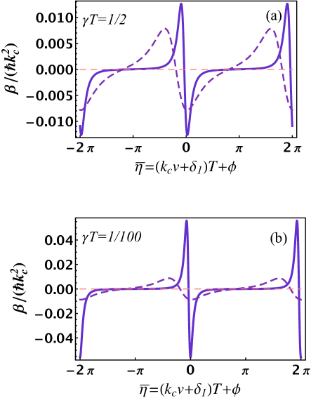
Figure 4: (Color online) Dependence of the friction coefficient $\beta/\hbar k_{c}^{2}$ on phase detuning $\bar{\eta}$ at (a) $\gamma T=1/2$ and (b) $\gamma T=1/100$. Each panel has three curves with different values of pulse area $\Theta$, $\Theta=\pi/10$ (solid purple line), $\Theta=\pi/2$ (dashed purple line), $\Theta=\pi$ (dashed pink line).

In Fig. 4 (a,b) we plot the dependence of friction coefficient $\beta$ (at $\theta_{1}=\theta_{2}$) (31) on the phase offset $\bar{\eta}$ at different values of $\gamma T$ and $\Theta$ at $\kappa=\kappa_{opt}$, optimally chosen for each pair of parameters $\gamma T$ and $\Theta$. It acquires the maximum value at $\bar{\eta}=\bar{\eta}_{\beta}$,

$$\bar{\eta}_{\beta}=-\cos^{-1}\left(\frac{b-\sqrt{8a^{2}+b^{2}}}{2a}\right)-\pi\kappa,$$ (32)

where

$$a=\cos(\pi\kappa)\left(\cos^{4}\left(\frac{\Theta}{4}\right)\cos^{2}(\pi\kappa)-\cos\left(\frac{\Theta}{2}\right)\right),$$ (33)

$$b=\cosh\left(\frac{\mu}{2}\right)\left(\cos^{2}\left(\frac{\Theta}{4}\right)\sin^{2}(\pi\kappa)+\sin^{4}\left(\frac{\Theta}{4}\right)\right).$$ (34)

For the case of non-equal pulse areas $\chi\neq\pi/4$)

$$\bar{\eta}_{\beta} = -\sec^{-1}\left({\frac{A^{2}+B^{2}}{A\left(C-D\right)+\sqrt{2}B\sqrt{CD-2\left(A^{2}+B^{2}\right)-C^{2}}}}\right),$$

$$D = \sqrt{8\left(A^{2}+B^{2}\right)+C^{2}},$$ (35)

where $A$, $B$ and $C$ are defined in (II.3, 30).

One can see (Fig.  4) that as the pulse repetition rate grows (smaller $\gamma T$), smaller values of single pulse area $\Theta$ lead to larger values of the friction coefficient $\beta$.

Notice however, that at very small values of $\gamma T\ll 1$ the momentum kick per pulse becomes smaller and the number of pulses needed to decelerate the atomic beam is increased.

At very large values of $\gamma T\gg 1$, while the friction coefficient $\beta$ vanishes, the momentum kick $\Delta p$ reaches its maximum. If the large value of $\gamma T\gg 1$ is due to the low pulse repetition rate, then the scattering force $F_{sc}=\Delta p/T$ also becomes smaller and the overall cooling time is increased.

For $\pi$-pulse and $\theta_{1}=\theta_{2}$ ($\chi=\pi/4$) the Eq. (32) reduces to

$$\beta_{\pi}=\frac{\hbar k_{c}^{2}}{2}\frac{\sinh\frac{\gamma T}{2}\sin^{2}(\pi\kappa)\cos^{3}(\pi\kappa)\sin(\bar{\eta}+\pi\kappa)}{(\cos^{3}(\pi\kappa)\cos(\bar{\eta}+\pi\kappa)-(\cos(2\pi\kappa)-2)\cosh\left(\frac{\gamma T}{2}\right))^{2}}.$$ (36)

At $\kappa=\frac{1}{2}$ (chosen in order to maximize the scattering force) the friction coefficient $\beta_{\pi}$ vanishes (similar to the case when $\gamma T\gg 1$). One can show that the friction coefficient at $\kappa=1/2$ and $\Theta=\pi$ turns to zero for arbitrary finite ratio of individual pulse areas $\theta_{1}/\theta_{2}$ and decay rates $\gamma_{1}/\gamma_{2}$ ($\chi\neq\pi/4$).

II.5 Finding the optimal cooling regime

Before discussing criteria for the optimal choice of FC parameters (single pulse area and pulse repetition rate ) we analyze the dependence of the scattering force profile on parameters $\gamma T$ and $\Theta$ at optimally chosen number of teeth $\kappa$ fitting into the energy gap between the two ground states. It is worth noticing, that the optimal value of $\kappa^{opt}$ is defined with an accuracy up the integer number, that is the values $\kappa^{opt}+n$, $n=0,1..$, where $\kappa^{opt}$ is defined from Eq. (20), are also optimal. Analysis in this section is carried out assuming the equal individual pulse areas $\theta_{1}=\theta_{2}$ and branching ratios $b_{1}=b_{2}$ ($\chi=\pi/4$).

In Fig.  5 we study the dependence of the scattering force $F_{sc}$ on phase offset parameter $\bar{\eta}$ at optimally chosen $\kappa$, Eq. (20), as the single pulse area $\Theta$ and the parameter $\mu$ vary.

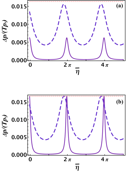
Figure 5: The dependence of the scattering force on the Doppler-shifted phase offset $\bar{\eta}$ at the optimal value of $\kappa=\kappa^{opt}$, chosen according to Eq. (21) at fixed value of $\mu=\gamma T$: panel (a)$\mu=1/2$, panel (b) $\mu=1/100$ and different values of effective single pulse area $\Theta$. Different curves correspond to the distinct values of single pulse areas: $\Theta=\frac{\pi}{10}$ (solid purple line), $\Theta=\frac{\pi}{2}$ (dashed blue line), $\Theta=\pi$ (dashed pink line).

One can see that at small $\mu=\gamma T$ in Fig. 5 the maxima of the scattering force is nearly independent on the pulse area $\Theta$ as long as $\Theta>\mu$. However, as $\Theta$ is increased the friction coefficient becomes smaller. As an example, at $\gamma T=1/100$ the amplitudes of scattering force corresponding to $\Theta=\pi/10$ and $\Theta=\pi/2$ are the same, but width of the peaks is smaller at $\Theta=\pi/10$.

At higher values of parameter $\mu$ the scattering force saturates at higher values of the pulse area $\Theta$. But the gradient of the scattering force is decreased.

At very small pulse areas $\Theta\rightarrow 0$ the scattering force vanishes (as well as the momentum kick $\Delta p$) regardless of the parameter $\gamma T$.

To summarize, at lower pulse repetition rates $\gamma T\gg 1$ and larger values of pulse area one can obtain larger momentum kick and smaller scattering force and compression rate. At larger pulse repetition rate ($\gamma T\ll 1$) and properly chosen $\Theta$ one can obtain the maximum of compression rate, but smaller momentum kick. In the first case the cooling time is increased and the compression of the velocity distribution is slow. In the second case the number of pulses needed to decelerate the beam is increased and the scattering force velocity capture range is decreased.

To find the opimal cooling regime one has to compromise between the fast slowing of the entire ensemble and its velocity distribution compression rate. In case when the scattering force rapidly vanishes in the vicinity of its maxima only the atoms within narrow groups of velocity are decelerated. Below we show that this problem can be mitigated. The spectral dependence of the scattering force can be varied in time, so that the positions of maxima follow the center of velocity distribution of the decelerating ensemble. In this case those atoms, which initially were outside of the scattering force velocity capture range and not decelerated will be eventually captured by the force profile being moved in the spectral domain (e.g. by changing the CEPO $\phi$).

However, if the initial atomic beam is too fast and (or) the velocity distribution is too wide, one can be interested initially in slowing down the ensemble, so that the cooling distance will be not too large. In this case one would prefer to have a broad scattering force profile (wide velocity capture range). The amplitude of the scattering force has to be large enough to mitigate the increase of cooling time and consequently cooling distance. This can be realized at larger pulse areas $\Theta$. For example, at $\mu\sim 1/2$, $\Theta\sim\pi/2$ for the atoms with the excited state lifetime $\tau\sim 15$ $ns$ at the laser field wavelength $\lambda=589$ $nm$, the velocity capture range $\Delta v_{cptr}$ is estimated by $\Delta v_{cptr}\sim 20$ $m/s$. The scattering force amplitude is quite the same as its maximum value, reached at $\Theta=\pi$.

At $\Theta=\pi$ the velocity capture range can be extended up to $\lambda/\tau_{p}$, where $\tau_{p}$ is the duration of pulse. For $\tau_{p}\sim 1$ $ps$ and $\lambda=589$ $nm$ the maximum velocity capture range is very broad $\Delta v_{cptr}^{max}\sim 5.89\times 10^{5}$ $m/s$.

If the intial velocity distribution is already narrow and (or) the central velocity value is not too high, the priority can be given to the fast velocity distribution compression.

The optimal set values of pulse area and pulse repetition rate can be chosen based on the initial velocity distribution, desired velocity compression rate and the limiting factors such as given cooling length and the laser power.

III Evolution of the velocity distribution

Now we turn to the dynamics of slowing down and cooling an entire atomic ensemble, characterized by some velocity distribution $f(v,t)$ (time-dependence is caused by radiative force).

III.1 No-cooling theorem for fixed FC parameters

Suppose that the positions of FC teeth remain fixed in the frequency domain during the deceleration. As the atoms slow down, they come in and out of resonances with different FC teeth. The gradient of the scattering force changes its sign (see Fig. 4) as the Doppler-shifted phase (velocity) vary. As a result the sustained cooling can not be realized if the positions of FC teeth remain fixed in frequency space during deceleration. This can be demonstrated as follows. Suppose the parameters of the frequency comb remain fixed. As a result of scattering $N$ pulses the atom with initial velocity $v_{i}$ will be decelerated to the final velocity $v_{f}$ determined from the implicit equation

$$Nv_{r} = \frac{2\csc^{2}\frac{\Theta}{2}\csc^{2}\pi\kappa}{k_{c}T\sinh\frac{\gamma T}{2}}\left(k_{c}T(v_{f}-v_{i})\cosh\frac{\gamma T}{2}\left(\cos^{4}\frac{\Theta}{4}\sin^{2}\pi\kappa+\sin^{4}\frac{\Theta}{4}\right)+\right.$$ (37)

$$\left.\cos\pi\kappa\left(\cos^{4}\frac{\Theta}{4}\cos^{2}\pi\kappa-\cos\frac{\Theta}{2}\right)(\sin(k_{c}Tv_{f}+\pi\kappa)-\sin(k_{c}Tv_{i}+\pi\kappa))\right).\qquad$$

where $v_{r}\equiv p_{r}/M$ is the recoil velocity. This equation was obtained by integrating Eq. (18).

Eq. (37) implies that the decrement in velocities would vary across the ensemble. Yet if we fix the change of velocity equal to the spacing between the teeth, $v_{f}=v_{i}-\lambda_{c}/T$, we find that the required number of pulses $N_{0}$ (or time $N_{0}T$),

$$N_{0}=\frac{2\lambda_{c}\csc^{2}\frac{\Theta}{2}\csc^{2}\pi\kappa}{Tv_{r}\sinh\frac{\gamma T}{2}}\cosh\frac{\gamma T}{2}\left(\cos^{4}\frac{\Theta}{4}\sin^{2}(\pi\kappa)+\sin^{4}\frac{\Theta}{4}\right),$$ (38)

does not dependent on the initial value $v_{i}$. This implies that if we start with a certain velocity distribution $f(v)$, the entire distribution is uniformly shifted by $-\lambda_{c}/T$ every $N_{0}$ pulses: $f(v)\rightarrow_{N_{0}}f(v+\lambda_{c}/T)$. Thus, the radiative force exerted by FC with fixed parameters does not lead to velocity compression — there is no cooling.

Notice that the above analysis has neglected variation of intensity across comb teeth. Also while there is no compression of the velocity distribution, there is a residual heating due to atomic recoil (this arises from treatments beyond our model, see, e.g., Ref. Metcalf and van der Straten (1999)).

III.2 Cooling via tuning the FC

In order to compress the velocity distribution, one has to maintain the positive gradient of the absolute value of the scattering force in the vicinity of the center of velocity distribution. To attain this condition, the scattering force profile has to follow the center of velocity distribution, moving towards the smaller velocities (frequencies) during the process of deceleration. In other words, the FC tooth closest to the atomic transition frequency $\omega_{eg_{1}}$ (in the reference frame moving with the center of velocity distribution) has to be somewhat red-detuned from $\omega_{eg_{1}}$. Tuning the positions of the FC teeth and consequently the scattering force profile can be achieved by tuning the phase of pulses during the cooling process Ilinova et al. (2011) .

Initially, we start with some velocity distribution $f(v,t=0)$. To optimize the number of cooled atoms, we focus on atoms with velocities grouped around the position of the maximum of $f(v,t=0)$, i.e. the most probable velocity $v_{mp}(t=0)$. Radiative force will cause both the distribution $f(v,t)$ and the most probable velocity $v_{mp}(t)$ to evolve in time.

To maximize the rate of compression, the friction coefficient needs to be kept at its maximum value at $v_{mp}(t)$. We may satisfy this requirement by tuning the phase offset $\phi(mT)=\Phi((m+1)T)-\Phi(mT)$ according to

$$\phi(t)=-\left(\delta+k_{c}v_{mp}(t)\right)T-\bar{\eta}_{\beta}\,,$$ (39)

where $\bar{\eta}_{\beta}$, Eq. (II.4), depends only on (time-independent) values of $\gamma T$, $\Theta$ and $\Delta_{12}/\omega_{rep}$. As $v_{mp}(t)$ becomes smaller due to the radiative force, the offset phase needs to be reduced.

We may find required pulse-to-pulse increment of the phase offset explicitly

$$\Delta\phi_{T}=\phi((m+1)T)-\phi(mT)=-\frac{k_{c}T}{M}\Delta p(\bar{\eta}_{\beta})\,.$$ (40)

When the phase offset is driven according to (40), there is a dramatic change in time-evolution of velocities of individual atoms. As the phase offset is varied over time, the entire frequency-comb structure shifts towards lower frequencies. As the teeth sweep through the velocity space, atomic $v(t)$ trajectories are “snow-plowed” by teeth, ultimately leading to narrow velocity spikes collected on the teeth. This emergence of “velocity comb” was discussed in Ref. Ilinova et al. (2011) for two-level system. Formally, we may separate initial velocities into groups

$$v_{mp}(t=0)+\left(2\pi(n-1)-\bar{\eta}_{\beta}\right)/k_{c}T<v(t=0)<v_{mp}(t=0)+\left(2\pi n-\bar{\eta}_{\beta}\right)/k_{c}T,n=0,\pm 1\ldots$$ (41)

The width of each velocity group is equal to the distance between neighboring teeth in velocity space, $2\pi/k_{c}T$. As a result of “snow-plowing”, the $n^{\mathrm{th}}$ group will be piled up at $v_{n}(t)=v_{mp}(t)+2\pi n/k_{c}T$. The final velocity spread of individual velocity groups will be limited by the Doppler temperature, $T_{D}=\hbar\gamma/2k_{B}$.

Figure 6: Time-evolution of velocity distribution for a thermal beam subjected to a coherent train of laser pulses. Pulse-to-pulse phase offset of the train is varied linearly in time as prescribed by Eq. (40). $N$ is the number of pulses. (a) Atomic and pulse train parameters are: $\gamma T=0.25$, $\Theta=\pi/2$. The optimal phase detuning is $\bar{\eta}=-1.23$. The center of initial velocity distribution is $v_{mp}=500$ m/s.

To illustrate the train-driven time-evolution for the entire ensemble, we consider a 1D thermal beam characterized by the initial velocity distribution

$$f(v,t=0)=\frac{v^{3}}{2\tilde{v_{0}}^{4}}\exp(-\frac{v^{2}}{2\tilde{v_{0}}^{2}}).$$ (42)

The most probable $v_{mp}$, average $v_{ave}$ and the r.m.s. $v_{rms}$ values are expressed in terms of $\widetilde{v}_{0}$ as

$$v_{mp}=\sqrt{3}\widetilde{v}_{0},$$

$$v_{ave}=\sqrt{\frac{9\pi}{8}}\widetilde{v}_{0},$$

$$v_{rms}=2\widetilde{v}_{0}.$$ (43)

$v_{mp}$ is the most probable velocity at $t=0$. A typical time-evolution of the velocity distribution is shown in Fig. 6. Local compression of velocity distribution happens near the points $v_{c}(t)+\lambda_{c}n/T$, $n=0,\pm 1..$, where $v_{c}$ is the time-dependent position of velocity distribution center. Clearly, velocity distribution, while initially being continuous, after a certain number of pulses develops a comb-like profile. This is the “velocity comb” of sharp peaks separated by equal intervals $\lambda_{c}/T$ in the velocity space.

IV Conclusion

In this paper we studied Doppler cooling of a three-level $\Lambda$-type system driven by a train of ultra-short laser pulses. Analytical expression for the scattering force was obtained and its dependence on the FC parameters was analyzed. The scattering force $F_{sc}$ is linearly proportional to the quasi-steady-state post-pulse excited state population. Its spectral (velocity) dependence exhibits periodic pattern mimicking the spectrum of the frequency comb. The contrast of the spectral profile of $F_{sc}$ is a function of the ratio between the excited state lifetime and the pulse repetition period, the effective single pulse area and the residual detunings $\bar{\delta_{j}}$ between the frequencies of individual transitions and nearest FC teeth. In a particular case when the pulse repetition period is much longer than the lifetime of the excited state, the spectral dependence of the scattering force reflects the broad-band spectral profile of a singe pulse.

The residual detunings $\bar{\delta}_{j}$ can be optimized to maximize the scattering force. At optimally chosen detunings the maximum of the scattering force is reached at single pulse area equal to $\pi$. However for $\pi$-pulses the spectral dependence of the scattering force is lost and consequently the friction coefficient vanishes. To optimize the cooling process one has to compromise between maximizing the scattering force and its velocity capture range and maintaining the sufficient gradient of the scattering force (friction coefficient). The spectral profile of the scattering force and consequently the friction coefficient can be varied in time to follow the moving center of the velocity distribution of decelerating ensemble. This can be realized by simply tuning the carrier envelope phase offset. Such manipulation enables sustained velocity distribution compression as the atoms slow down. As a result, initially smooth velocity distribution of a thermal beam evolves into a series of narrow groups of velocities separated by $\lambda_{c}/T$, so called “velocity comb”.

References

- Hansch and Schawlow (1975) T. Hansch and A. Schawlow, Opt. Comm. 13, 68 (1975).
- Minogin and Letokhov (1987) V. Minogin and V. Letokhov, Laser Light Pressure on Atoms (Gordon and Breach, New York, 1987).
- Metcalf and van der Straten (1999) H. J. Metcalf and P. van der Straten, Laser Cooling and Trapping (Springer,New York, 1999).
- Berman and Malinovsky (2010) P. R. Berman and V. S. Malinovsky, Principles of Laser Spectroscopy and Quantum Optics (Princeton University Press, 2010).
- Hoffnagle (1988) J. Hoffnagle, J. Opt. Lett. 13, 102 (1988).
- Strohmeier et al. (1989) Strohmeier et al., Opt. Comm. 73, 451 (1989).
- Watanabe et al. (1996) M. Watanabe, R. Ohmukai, U. Tanaka, K. Hayasaka, H. Imajo, and S. Urabe, J. Opt. Soc. Am. B 13, 2377 (1996).
- Kielpinski (2006) D. Kielpinski, Phys. Rev. A 73, 063407 (2006).
- Ilinova et al. (2011) E. Ilinova, M. Ahmad, and A. Derevianko, ArXiv e-prints (2011), eprint 1105.0665.
- Kazantsev (1974) A. Kazantsev, Zh. Exp. Theor. Fiz. 66, 1599 (1974).
- Noelle et al. (1996) B. Noelle, H. Noelle, J. Schmand, and H. J. Andra, Europhys. Lett. 33, 261 (1996).
- Goepfert et al. (1997) A. Goepfert, I. Bloch, D. Haubrich, F. Lison, R. Schütze, R. Wynands, and D. Meschede, Phys. Rev. A 56, R3354 (1997), URL http://link.aps.org/doi/10.1103/PhysRevA.56.R3354.
- Söding et al. (1997) J. Söding, R. Grimm, Y. B. Ovchinnikov, P. Bouyer, and C. Salomon, Phys. Rev. Lett. 78, 1420 (1997), URL http://link.aps.org/doi/10.1103/PhysRevLett.78.1420.
- Schibli et al. (2008) T. R. Schibli, I. Hartl, D. C. Yost, M. J. Martin, A. Marcinkevicius, M. E. Fermann, and J. Ye, Nat. Photon. 2, 355 (2008).
- Adler et al. (2009) F. Adler, K. C. Cossel, M. J. Thorpe, I. Hartl, M. E. Fermann, and J. Ye, Opt. Lett. 34, 1330 (2009).
- Vodopyanov et al. (2011) K. Vodopyanov, E. Sorokin, I. T. Sorokina, and P. G. Schunemann, Opt. Lett. 36, 2275 (2011).
- Marian et al. (2004) A. Marian, M. C. Stowe, J. R. Lawall, D. Felinto, and J. Ye, Science 17, 2063 (2004).
- Prudnikov and Arimondo (2003) O. N. Prudnikov and E. Arimondo, J. Opt. Soc. Am. B 20, 909 (2003).
- Aspect et al. (1988) A. Aspect, E. Arimondo, R. Kaiser, N. Vansteenkiste, and C. Cohen-Tannoudji, Phys. Rev. Lett. 61, 826 (1988), URL http://link.aps.org/doi/10.1103/PhysRevLett.61.826.
- Kasevich and Chu (1992) M. Kasevich and S. Chu, Phys. Rev. Lett. 69, 1741 (1992), URL http://link.aps.org/doi/10.1103/PhysRevLett.69.1741.
- Gupta et al. (1993) R. Gupta, C. Xie, S. Padua, H. Batelaan, and H. Metcalf, Phys. Rev. Lett. 71, 3087 (1993).
- Aspect et al. (1986) A. Aspect, J. Dalibard, A. Heidmann, C. Salomon, and C. Cohen-Tannoudji, Phys. Rev. Lett. 57, 1688 (1986), URL http://link.aps.org/doi/10.1103/PhysRevLett.57.1688.
- Zhu et al. (1991) M. Zhu, C. W. Oates, and J. L. Hall, Phys. Rev. Lett. 67, 46 (1991).
- Schröder et al. (1990) S. Schröder et al., Phys. Rev. Lett. 64, 2901 (1990).
- Miesner et al. (1996) H.-J. Miesner et al., Phys. Rev. Lett. 77, 623 (1996).
- Ilinova and Derevianko (2012) E. Ilinova and A. Derevianko, arXiv:1203.0034 (2012).
- Harris (1997) S. E. Harris, Physics Today 50, 36 (1997).
- Moreno and Vianna (2011) M. P. Moreno and S. S. Vianna, J. Opt. Soc. Am. B 28, 1124 (2011).
- Soares and de Araujo (2007) A. A. Soares and L. E. E. de Araujo, Phys. Rev. A 76, 043818 (2007), URL http://link.aps.org/doi/10.1103/PhysRevA.76.043818.
- Soares and Araujo (2010) A. Soares and E. E. Araujo, J. Phys. B 43, 085003 (2010).