Worst-case Optimal Join Algorithms

Abstract

Efficient join processing is one of the most fundamental and well-studied tasks in database research. In this work, we examine algorithms for natural join queries over many relations and describe a novel algorithm to process these queries optimally in terms of worst-case data complexity. Our result builds on recent work by Atserias, Grohe, and Marx, who gave bounds on the size of a full conjunctive query in terms of the sizes of the individual relations in the body of the query. These bounds, however, are not constructive: they rely on Shearer’s entropy inequality which is information-theoretic. Thus, the previous results leave open the question of whether there exist algorithms whose running time achieve these optimal bounds. An answer to this question may be interesting to database practice, as it is known that any algorithm based on the traditional select-project-join style plans typically employed in an RDBMS are asymptotically slower than the optimal for some queries. We construct an algorithm whose running time is worst-case optimal for all natural join queries. Our result may be of independent interest, as our algorithm also yields a constructive proof of the general fractional cover bound by Atserias, Grohe, and Marx without using Shearer’s inequality. This bound implies two famous inequalities in geometry: the Loomis-Whitney inequality and the Bollobás-Thomason inequality. Hence, our results algorithmically prove these inequalities as well. Finally, we discuss how our algorithm can be used to compute a relaxed notion of joins.

1 Introduction

Recently, Grohe and Marx [13] and Atserias, Grohe, and Marx [4] (AGM’s results henceforth) derived tight bounds on the number of output tuples of a full conjunctive query in terms of the sizes of the relations mentioned in the query’s body. As query output size estimation is fundamentally important for efficient query processing, these results have generated a great deal of excitement.

To understand the spirit of AGM’s results, consider the following example where we have a schema with three attributes, $A$, $B$, and $C$, and three relations, $R(A,B)$, $S(B,C)$ and $T(A,C)$, defined over those attributes. Consider the following natural join query:

$$q=R\Join S\Join T$$ (1)

Let $q(I)$ denote the set of tuples that is output from applying $q$ to a database instance $I$, that is the set of triples of constants $(a,b,c)$ such that $R(ab)$, $S(bc)$, and $T(ac)$ are in $I$. Our goal is to bound the number of tuples returned by $q$ on $I$, denoted by $|q(I)|$, in terms of $|R|$, $|S|$, and $|T|$. For simplicity, let us consider the case when $|R|=|S|=|T|=N$. A straightforward bound is $|q(I)|\leq N^{3}$. One can obtain a better bound by noticing that any pair-wise join (say $R\Join S$) will contain $q(I)$ in it as $R$ and $S$ together contain all attributes (or they “cover” all the attributes). This leads to the bound $|q(I)|\leq N^{2}$. AGM showed that one can get a better upper bound of $|q(I)|\leq N^{3/2}$ by generalizing the notion of cover to a so-called “fractional cover” (see Section 2). Moreover, this estimate is tight in the sense that for infinitely many values of $N$, one can find a database instance $I$ that for which $|q(I)|=N^{3/2}$. These non-trivial estimates are exciting to database researchers as they offer previously unknown, nontrivial methods to estimate the cardinality of a query result – a fundamental problem to support efficient query processing.

More generally, given an arbitrary natural-join query $q$ and given the sizes of input relations, the AGM method can generate an upper bound $U$ such that $|q(I)|\leq U$, where $U$ depends on the “best” fractional cover of the attributes. This “best” fractional cover can be computed by a linear program (see Section 2 for more details). Henceforth, we refer to this inequality as the AGM’s fractional cover inequality, and the bound $U$ as the AGM’s fractional cover bound. They also show that the bound is essentially optimal in the sense that for infinitely many sizes of input relations, there exists an instance $I$ such that each relation in $I$ is of the prescribed size and $|q(I)|=U$.

AGM’s results leave open whether one can compute the actual set $q(I)$ in time $O(U)$. In fact, AGM observe this issue and presented an algorithm that computes $q(I)$ with a running time of $O(|q|^{2}\cdot U\cdot N)$ where $N$ is the cardinality of the largest input relation and $|q|$ denotes the size of the query $q$. AGM establish that their join-project plan can in some cases be super-polynomially better than any join-only plan. However, AGM’s join algorithm is not optimal. Even on the above example of (1), we can construct a family of database instances $I_{1},I_{2},\dots,I_{N},\dots,$ such that in the $N$th instance $I_{N}$ we have $|R|=|S|=|T|=N$ and both AGM’s algorithm and any join-only plan take $\Omega(N^{2})$-time even though from AGM’s bound we know that $|q(I)|\leq U=N^{3/2}$, which is the best worst-case run-time one can hope for.

The $\sqrt{N}$-gap on a small example motivates our central question. In what follows, natural join queries are defined as the join of a set of relations $R_{1},\dots,R_{m}$.

Optimal Worst-case Join Evaluation Problem (Optimal Join Problem). Given a fixed database schema $\bar{R}=\left\{R_{i}(\bar{A}_{i})\right\}_{i=1}^{m}$ and an $m$-tuple of integers $\bar{N}=(N_{1},\dots,N_{m})$. Let $q$ be the natural join query joining the relations in $\bar{R}$ and let $I(\bar{N})$ be the set of all instances such that $|R_{i}^{I}|=N_{i}$ for $i=1,\dots,m$. Define $U=\sup_{I\in I(\bar{N})}|q(I)|$. Then, the optimal worst-case join evaluation problem is to evaluate $q$ in time $O(U+\sum_{i=1}^{m}N_{i})$.

Since any algorithm to produce $q(I)$ requires time at least $|q(I)|$, an algorithm that solves the above problem would have an optimal worst-case data-complexity. (Note that we are mainly concerned with data complexity and thus the $O(U)$ bound above ignores the dependence on $|q|$. Our results have a small $O(|q|)$ factor.)

Implicitly, this problem has been studied for over three decades: a modern RDBMS use decades of highly tuned algorithms to efficiently produce query results. Nevertheless, as we described above, such systems are asymptotically suboptimal – even in the above simple example of (1). Our main result is an algorithm that achieves asymptotically optimal worst-case running times for all conjunctive join queries.

We begin by describing connections between AGM’s inequality and a family of inequalities in geometry. In particular, we show that the AGM’s inequality is equivalent to the discrete version of a geometric inequality proved by Bollóbas and Thomason ([7], Theorem 2). This equivalence is shown in Section 3.

Our ideas for an algorithm solving the optimal join problem begin by examining a special case of the Bollóbas-Thomason (BT) inequality: the classic Loomis-Whitney (LW) inequality [24]. The LW inequality bounds the measure of an $n$-dimensional set in terms of the measures of its $(n-1)$-dimensional projections onto the coordinate hyperplanes. The query (1) and its bound $|q(I)|\leq\sqrt{|R||S||T|}$ is exactly the LW inequality with $n=3$ applied to the discrete measure. Our algorithmic development begins with a slight generalization of the query $q$ in (1). We describe an algorithm for join queries which have the same format as in the LW inequality setup with $n\geq 3$. In particular, we consider “LW instances” of the optimal join problem, where the query is to join $n$ relations whose attribute sets are all the distinct $(n-1)$-subsets of a universe of $n$ attributes. Since the LW inequality is tight, and our join algorithm has running time that is asymptotically data-optimal for this class of queries (e.g., $O(N^{3/2})$ in our motivating example), our algorithm is data-complexity optimal in the worst case for LW instances.

Our algorithm for LW instances exhibits a key twist compared to a conventional join algorithm. The twist is that the join algorithm partitions the values of the join key on each side of the join into two sets: those values that are heavy and those values that are light. Intuitively, a value of a join key is heavy if its fanout is high enough so that joining all such join keys could violate the size bound (e.g., $N^{3/2}$ above). The art is selecting the precise fanout threshold for when a join key is heavy. This per-tuple choice of join strategy is not typically done in standard RDBMS join processing.

Building on our algorithm for LW instances, we next describe our main result: an algorithm to solve the optimal join problem for all join queries. In particular, we design an algorithm for evaluating join queries which not only proves AGM’s fractional cover inequality without using the information-theoretic Shearer’s inequality, but also has a running time that is linear in the bound (modulo pre-processing time). As AGM’s inequality implies the BT and LW inequalities, our result is the first algorithmic proof of these geometric inequalities as well. To do this, we must carefully select which projections of relations to join and in which order our algorithm joins relations on a “per tuple” basis as in the LW-instance case. Our algorithm computes these orderings, and then at each stage it performs an algorithm that is similar to the algorithm we used for LW instances.

Our example also shows that standard join algorithms are suboptimal, the question is, when do classical RDBMS algorithms have higher worst-case run-time than our proposed approach? AGM’s analysis of their join-project algorithm leads to a worst case run-time complexity that is a factor of the largest relation worse than the AGM’s bound. To investigate whether AGM’s analysis is tight or not, we ask a sharper variant of this question: Given a query $q$ does there exist a family of instances $I$ such that our algorithm runs asymptotically faster than a standard binary-join-based plan or AGM’s join-project plan? We give a partial answer to this question by describing a sufficient syntactic condition for the query $q$ such that for each $k\geq 2$, we can construct a family of instances where each relation is of size $N$ such that any binary-join plan as well as AGM’s algorithm will need time $\Omega(N^{2}/k^{2})$, while the fractional cover bound is $O(N^{1+1/(k-1)})$ – an asymptotic gap. We then show through a more detailed analysis that our algorithm on these instances takes $O(k^{2}N)$-time.

We consider several extensions and improvements of our main result. In terms of the dependence on query size, our algorithms are also efficient (at most linear in $|q|$, which is better than the quadratic dependence in AGM) for full queries, but they are not necessarily optimal. In particular, if each relation in the schema has arity $2$, we are able to give an algorithm with better query complexity than our general algorithm. This shows that in general our algorithm’s dependence on the factors of the query is not the best possible. We also consider computing a relaxed notion of joins and give worst-case optimal algorithms for this problem as well.

Outline

The remainder of the paper is organized as follows: in the rest of this section, we describe related work. In Section 2 we describe our notation and formulate the main problem. Section 3 proves the connection between AGM’s inequality and BT inequality. In Section 4 we present a data-optimal join algorithm for LW instances, and then extend this to arbitrary join queries in Section 5. We discuss the limits of performance of prior approaches and our approach in more detail in Section 6. In Section 7, we describe several extensions. We conclude in Section 8.

Related Work

Grohe and Marx [13] made the first (implicit) connection between fractional edge cover and the output size of a conjunctive query. (Their results were stated for constraint satisfaction problems.) Atserias, Grohe, and Marx [4] extended Grohe and Marx’s results in the database setting.

The first relevant AGM’s result is the following inequality. Consider a join query over relations $R_{e}$, $e\in E$, where $E$ is a collection of subsets of an attribute “universe” $V$, and relation $R_{e}$ is on attribute set $e$. Then, the number of output tuples is bounded above by $\prod_{e\in E}|R_{e}|^{x_{e}}$, where $\mathbf{x}=(x_{e})_{e\in E}$ is an arbitrary fractional cover of the hypergraph $H=(V,E)$.

They also showed that this bound is tight. In particular, for infinitely many positive integers $N$ there is a database instance with $|R_{e}|=N$, $\forall e\in E$, and the upper bound gives the actual number of output tuples. When the sizes $|R_{e}|$ were given as inputs to the (output size estimation) problem, obviously the best upper bound is obtained by picking the fractional cover $\mathbf{x}$ which minimizes the linear objective function $\sum_{e\in E}(\log|R_{e}|)\cdot x_{e}$. In this “size constrained” case, however, their lower bound is off from the upper bound by a factor of $2^{n}$, where $n$ is the total number of attributes. AGM also presented an inapproximability result which justifies this gap. Note, however, that the gap is only dependent on the query size and the bound is still asymptotically optimal in the data-complexity sense.

The second relevant result from AGM is a join-project plan with running time $O\left(|q|^{2}N_{\text{max}}^{1+\sum x_{e}}\right)$, where $N_{\text{max}}$ is the maximum size of input relations and $|q|=|V|\cdot|E|$ is the query size.

The AGM’s inequality contains as a special case the discrete versions of two well-known inequalities in geometry: the Loomis-Whitney (LW) inequality [24] and its generalization the Bollobás-Thomason (BT) inequality [7]. There are two typical proofs of the discrete LW and BT inequalities. The first proof is by induction using Hölder’s inequality [7]. The second proof (see Lyons and Peres [25]) essentially uses “equivalent” entropy inequalities by Han [15] and its generalization by Shearer [8], which was also the route Grohe and Marx [13] took to prove AGM’s bound. All of these proofs are non-constructive.

There are many applications of the discrete LW and BT inequalities. The $n=3$ case of the LW inequality was used to prove communication lower bounds for matrix multiplication on distributed memory parallel computers [19]. The inequality was used to prove submultiplicativity inequalities regarding sums of sets of integers [14]. In [23], a special case of BT inequality was used to prove a network-coding bound. Recently, some of the authors of this paper have used our algorithmic version of the LW inequality to design a new sub-linear time decodable compressed sensing matrices [10] and efficient pattern matching algorithms [28].

Inspired by AGM’s results, Gottlob, Lee, and Valiant [11] provided bounds for conjunctive queries with functional dependencies. For these bounds, they defined a new notion of “coloring number” which comes from the dual linear program of the fractional cover linear program. This allowed them to generalize previous results to all conjunctive queries, and to study several problems related to tree-width.

Join processing algorithms are one of the most studied algorithms in database research. A staggering number of variants have been considered, we list a few: Block-Nested loop join, Hash-Join, Grace, Sort-merge (see Grafe [12] for a survey). Conceptually, it is interesting that none of the classical algorithms consider performing a per-tuple cardinality estimation as our algorithm does. It is interesting future work to implement our algorithm to better understand its performance.

Related to the problem of estimating the size of an output is cardinality estimation. A large number of structures have been proposed for cardinality estimation [17, 30, 9, 1, 21, 20], they have all focused on various sub-classes of queries and deriving estimates for arbitrary query expressions has involved making statistical assumptions such as the independence and containment assumptions which result in large estimation errors [18]. Follow-up work has considered sophisticated probability models, Entropy-based models [26, 32] and graphical models [33]. In contrast, in this work we examine the worst case behavior of algorithms in terms of its cardinality estimates. In the special case when the join graph is acyclic, there are several known results which achieve (near) optimal run time with respect to the output size [29, 35].

On a technical level, the work adaptive query processing is related, e.g., Eddies [5] and RIO [6]. The main idea is that to compensate for bad statistics, the query plan may adaptively be changed (as it better understands the properties of the data). While both our method and the methods proposed here are adaptive in some sense, our focus is different: this body of work focuses on heuristic optimization methods, while our focus is on provable worst-case running time bounds. A related idea has been considered in practice: heuristics that split tuples based on their fanout have been deployed in modern parallel databases to handle skew [36]. This idea was not used to theoretically improve the running time of join algorithms. We are excited by the fact that a key mechanism used by our algorithm has been implemented in a modern commercial system.

2 Notation and Formal Problem Statement

We assume the existence of a set of attribute names $\mathcal{A}=A_{1},\dots,A_{n}$ with associated domains $\mathbf{D}_{1},\dots,\mathbf{D}_{n}$ and infinite set of relational symbols $R_{1},R_{2},\dots$. A relational schema for the symbol $R_{i}$ of arity $k$ is a tuple $\bar{A}_{i}=(A_{i_{1}},\dots,A_{i_{k}})$ of distinct attributes that defines the attributes of the relation. A relational database schema is a set of relational symbols and associated schemas denoted by $R_{1}(\bar{A}_{1}),\dots,R_{m}(\bar{A}_{m})$. A relational instance for $R(A_{i_{1}},\dots,A_{i_{k}})$ is a subset of $\mathbf{D}_{i_{1}}\times\dots\times\mathbf{D}_{i_{k}}$. A relational database $I$ is an instance for each relational symbol in schema, denoted by $R_{i}^{I}$. A natural join query (or simply query) $q$ is specified by a finite subset of relational symbols $q\subseteq\mathbb{N}$, denoted by $\Join_{i\in q}R_{i}$. Let $\bar{A}(q)$ denote the set of all attributes that appear in some relation in $q$, that is $\bar{A}(q)=\{A\mid A\in\bar{A}_{i}\text{ for some }i\in q\}$. Given a tuple $\mathbf{t}$ we will write $\mathbf{t}_{\bar{A}}$ to emphasize that its support is the attribute set $\bar{A}$. Further, for any $\bar{S}\subset\bar{A}$ we let $\mathbf{t}_{\bar{S}}$ denote $\mathbf{t}$ restricted to $\bar{S}$. Given a database instance $I$, the output of the query $q$ on $I$ is denoted $q(I)$ and is defined as

$$q(I)\stackrel{{\scriptstyle\mathrm{def}}}{{=}}\left\{\mathbf{t}\in\mathbf{D}^{\bar{A}(q)}\ |\ \mathbf{t}_{\bar{A}_{i}}\in R^{I}_{i}\text{ for each }i\in q\right\}$$

where $\mathbf{D}^{\bar{A}(q)}$ is a shorthand for $\times_{i:A_{i}\in\bar{A}(q)}\mathbf{D}_{i}$.

We also use the notion of a semijoin: Given two relations $R(\bar{A})$ and $S(\bar{B})$ their semijoin $R\lJoin S$ is defined by

$$R\lJoin S\stackrel{{\scriptstyle\mathrm{def}}}{{=}}\left\{\mathbf{t}\in R:\exists\mathbf{u}\in S\text{ s.t. }\mathbf{t}_{\bar{A}\cap\bar{B}}=\mathbf{u}_{\bar{A}\cap\bar{B}}\right\}.$$

For any relation $R(\bar{A})$, and any subset $\bar{S}\subseteq\bar{A}$ of its attributes, let $\pi_{\bar{S}}(R)$ denote the projection of $R$ onto $\bar{S}$, i.e.

$$\pi_{\bar{S}}(R)=\left\{\mathbf{t}_{\bar{S}}\ |\ \exists\mathbf{t}_{\bar{A}\setminus\bar{S}},(\mathbf{t}_{\bar{S}},\mathbf{t}_{\bar{A}\setminus\bar{S}})\in R\right\}.$$

For any tuple $\mathbf{t}_{\bar{S}}$, define the $\mathbf{t}_{\bar{S}}$-section of $R$ as

$$R[\mathbf{t}_{\bar{S}}]=\pi_{\bar{A}\setminus\bar{S}}(R\lJoin\{\mathbf{t}_{\bar{S}}\}).$$

From Join Queries to Hypergraphs

A query $q$ on attributes $\bar{A}(q)$ can be viewed as a hypergraph $H=(V,E)$ where $V=\bar{A}(q)$ and there is an edge $e_{i}=\bar{A}_{i}$ for each $i\in q$. Let $N_{e}=|R_{e}|$ be the number of tuples in $R_{e}$. From now on we will use the hypergraph and the original notation for the query interchangeably.

We use this hypergraph to introduce the fractional edge cover polytope that plays a central role in our technical developments. The fractional edge cover polytope defined by $H$ is the set of all points $\mathbf{x}=(x_{e})_{e\in E}\in\mathbb{R}^{E}$ such that

$$\sum_{v\in e}x_{e} \geq 1,\ \text{for any $v\in V$}$$

$$x_{e} \geq 0,\text{for any $e\in E$}$$

Note that the solution $x_{e}=1$ for $e\in E$ is always feasible for hypergraphs representing join queries. A point $\mathbf{x}$ in the polytope is also called a fractional (edge) cover solution of the hypergraph $H$.

Atserias, Grohe, and Marx [4] establish that, for any point $\mathbf{x}=(x_{e})_{e\in E}$ in the fractional edge cover polytope

$$|\Join_{e\in E}R_{e}|\leq\prod_{e\in E}N_{e}^{x_{e}}.$$ (2)

The bound is proved nonconstructively using Shearer’s entropy inequality [8]. However, AGM provide an algorithm based on join-project plans that runs in time $O(|q|^{2}\cdot N_{\max}^{1+\sum_{e}x_{e}})$ where $N_{\max}=\max_{e\in E}N_{e}$. They observed that for a fixed hypergraph $H$ and given sizes $N_{e}$ the bound (2) can be minimized by solving the linear program which minimizes the linear objective $\sum_{e}(\log N_{e})\cdot x_{e}$ over fractional edge cover solutions $\mathbf{x}$. (Since in linear time we can figure out if we have an empty relation, and hence an empty output), for the rest of the paper we are always going to assume that $N_{e}\geq 1$.) Thus, the formal problem that we consider recast in this language is:

Definition 2.1 (OJ Problem – Optimal Join Problem).

With the notation above, design an algorithm to compute $\Join_{e\in E}R_{e}$ with running time

$$O\left(f(|V|,|E|)\cdot\left(\prod_{e\in E}N_{e}^{x_{e}}+\sum_{e\in E}N_{e}\right)\right).$$

Here $f(|V|,|E|)$ is ideally a polynomial with (small) constant degree, which only depends on the query size. The linear term $\sum_{e\in E}N_{e}$ is to read the input. Hence, such an algorithm would be data-optimal in the worst case.

We recast our motivating example from the introduction in our notation. Recall we are given, $R(A,B),S(B,C),T(A,C)$, so $V=\{A,B,C\}$ and three edges corresponding each to $R$, $S$, and $T$, which are $E=\{\{A,B\}$, $\{B,C\}$, $\{A,C\}\}$ respectively. Thus, $|V|=3$ and $|E|=3$. If we are given that $N_{e}=N$, one can check that the optimal solution to the LP is $x_{e}=\frac{1}{2}$ for $e\in E$ which has the objective value $\frac{3}{2}\log N$; in turn, this gives $\sup_{I\in I(\bar{N})}|q(I)|\leq N^{3/2}$ (recall $I(\bar{N})=\{I:|R_{e}^{I}|=N_{e}\text{ for }e\in E\}$).

Example 2.2.

Given an even integer $N$, we construct an instance $I_{N}$ such that (1) $|R^{I_{N}}|=|S^{I_{N}}|=|T^{I_{N}}|=N$, (2) $|R\Join S|=|R\Join T|=|S\Join T|=N^{2}/4+N/2$, and (3) $|R\Join S\Join T|=0$. The following instance satisfies all three properties:

$$R^{I_{N}}=S^{I_{N}}=T^{I_{N}}=\left\{(0,j)\right\}_{j=1}^{N/2}\cup\left\{(j,0)\right\}_{j=1}^{N/2}.$$

For example,

$$R\Join S=\{(i,0,j)\}_{i,j=1}^{N/2}\cup\{(0,i,0)\}_{i=1,\dots,N/2}$$

and $R\Join S\Join T=\emptyset$. Thus, any standard join-based algorithm takes time $\Omega(N^{2})$. We show later that AGM’s algorithm takes $\Omega(N^{2})$-time too. Recall that the AGM bound for this instance is $O(N^{3/2})$, and our algorithm thus takes time $O(N^{3/2})$. In fact, as shall be shown later, on this particular family of instances both of our algorithms take only $O(N)$ time.

3 Connections to Geometric Inequalities

We describe the Bollobás-Thomason (BT) inequality from discrete geometry and prove that BT inequality is equivalent to AGM’s inequality. We then look at a special case of BT inequality, the Loomis-Whitney (LW) inequality, from which our algorithmic development starts in the next section. We state the BT inequality:

Theorem 3.1 (Discrete Bollobás-Thomason (BT) Inequality).

Let $S\subset\mathbb{Z}^{n}$ be a finite set of $n$-dimensional grid points. Let $\mathcal{F}$ be a collection of subsets of $[n]$ in which every $i\in[n]$ occurs in exactly $d$ members of $\mathcal{F}$. Let $S_{F}$ be the set of projections $\mathbb{Z}^{n}\to\mathbb{Z}^{F}$ of points in $S$ onto the coordinates in $F$. Then, $|S|^{d}\leq\prod_{F\in\mathcal{F}}|S_{F}|$.

To prove the equivalence between BT inequality and the AGM bound, we first need a simple observation.

Lemma 3.2.

Consider an instance of the OJ problem consisting of a hypergraph $H=(V,E)$, a fractional cover $\mathbf{x}=(x_{e})_{e\in E}$ of $H$, and relations $R_{e}$ for $e\in E$. Then, in linear time we can transform the instance into another instance $H^{\prime}=(V,E^{\prime})$, $\mathbf{x}^{\prime}=(x^{\prime}_{e})_{e\in E^{\prime}}$, $(R^{\prime}_{e})_{e\in E^{\prime}}$, such that the following properties hold:

• $\mathbf{x}^{\prime}$ is a “tight” fractional edge cover of the hypergraph $H^{\prime}$, namely $\mathbf{x}^{\prime}\geq 0$ and

  $$\sum_{e\in E^{\prime}:v\in e}x^{\prime}_{e}=1,\ \ \text{ for every }v\in V.$$

• The two problems have the same answer:

  $$\Join_{e\in E}R_{e}=\ \Join_{e\in E^{\prime}}R^{\prime}_{e}.$$

• AGM’s bound on the transformed instance is at least as good as that of the original instance:

  $$\prod_{e\in E^{\prime}}|R^{\prime}_{e}|^{x^{\prime}_{e}}\leq\prod_{e\in E}|R_{e}|^{x_{e}}.$$

Proof.

We describe the transformation in steps. At each step properties (b) and (c) are kept as invariants. After all steps are done, (a) holds.

While there still exists some vertex $v\in V$ such that $\sum_{e\in E:v\in e}x_{e}>1$, i.e. $v$’s constraint is not tight, let $f$ be an arbitrary hyperedge $f\in E$ such that $v\in f$. Partition $f$ into two parts $f=f_{t}\cup f_{\neg t}$, where $f_{t}$ consists of all vertices $u\in f$ such that $u$’s constraint is tight, and $f_{\neg t}$ consist of vertices $u\in f$ such that $u$’s constraint is not tight. Note that $v\in f_{\neg t}$.

Define $\rho=\min\left\{x_{f},\min_{u\in f_{\neg t}}\left\{\sum_{e:u\in e}x_{e}-1\right\}\right\}.$ This is the amount which, if we were able to reduce $x_{f}$ by $\rho$ then we will either turn $x_{f}$ to $0$ or make some constraint for $u\in f_{\neg t}$ tight. However, reducing $x_{f}$ might violate some already tight constraint $u\in f_{t}$. The trick is to “break” $f$ into two parts.

We will set $E^{\prime}=E\cup\{f_{t}\}$, create a “new” relation $R^{\prime}_{f_{t}}=\pi_{f_{t}}(R_{f})$, and keep all the old relations $R^{\prime}_{e}=R_{e}$ for all $e\in E$. Set the variables $x^{\prime}_{e}=x_{e}$ for all $e\in E-\{f\}$ also. The only two variables which have not been set are $x^{\prime}_{f}$ and $x^{\prime}_{f_{t}}$. We set them as follows.

• When $x_{f}\leq\min_{u\in f_{\neg t}}\left\{\sum_{e:u\in e}x_{e}-1\right\}$, set $x^{\prime}_{f}=0$ and $x^{\prime}_{f_{t}}=x_{f}$.

• When $x_{f}>\min_{u\in f_{\neg t}}\left\{\sum_{e:u\in e}x_{e}-1\right\}$, set $x^{\prime}_{f}=x_{f}-\rho$ and $x^{\prime}_{f_{t}}=\rho$.

Either way, it can be readily verified that the new instance is a legitimate OJ instance satisfying properties (b) and (c). In the first case, some positive variable in some non-tight constraint has been reduced to $0$. In the second case, at least one non-tight constraint has become tight. Once we change a variable $x_{f}$ (essentially “break” it up into $x^{\prime}_{f_{t}}$ and $x^{\prime}_{f}$) we won’t touch it again. Hence, after a linear number of steps in $|V|$, we will have all tight constraints. ∎

With this technical observation, we can now connect the two families of inequalities:

Proposition 3.3.

BT inequality and AGM’s fractional cover bound are equivalent.

Proof.

To see that AGM’s inequality implies BT inequality, we think of each coordinate as an attribute, and the projections $S_{F}$ as the input relations. Set $x_{F}=1/d$ for each $F\in\mathcal{F}$. It follows that $\mathbf{x}=(x_{F})_{F\in\mathcal{F}}$ is a fractional cover for the hypergraph $H=([n],\mathcal{F})$. AGM’s bound then implies that $|S|\leq\prod_{F\in\mathcal{F}}|S_{F}|^{1/d}$.

Conversely, consider an instance of the OJ problem with hypergraph $H=(V,E)$ and a rational fractional cover $\mathbf{x}=(x_{e})_{e\in E}$ of $H$. First, by Lemma 3.2, we can assume that all cover constraints are tight, i.e.,

$$\sum_{e:v\in e}x_{e}=1,\ \ \text{ for any }v\in V.$$

By standard arguments, it can be shown that all the “new” $x_{e}$ are rational values (even if the original values were not). Second, by writing all variables $x_{e}$ as $d_{e}/d$ for a positive common denominator $d$ we obtain

$$\sum_{e:v\in e}d_{e}=d,\ \ \text{ for any }v\in V.$$

Now, create $d_{e}$ copies of each relation $R_{e}$. Call the new relations $R^{\prime}_{e}$. We obtain a new hypergraph $H^{\prime}=(V,E^{\prime})$ where every attribute $v$ occurs in exactly $d$ hyperedges. This is precisely the Bollóbas-Thomason’s setting of Theorem 3.1. Hence, the size of the join is bounded above by $\prod_{e\in E^{\prime}}|R^{\prime}_{e}|^{1/d}=\prod_{e\in E}|R_{e}|^{d_{e}/d}=\prod_{e\in E}|R_{e}|^{x_{e}}.$ ∎

Loomis-Whitney

We now consider a special case of BT (or AGM), the discrete version of a classic geometric inequality called the Loomis-Whitney inequality [24]. The setting is that for $n\geq 2$, $V=[n]$ and $E=\binom{V}{|V|-1}$. In this case $x_{e}=1/(|V|-1),\forall e\in E$ is a fractional cover solution for $(V,E)$, and LW showed the following:

Theorem 3.4 (Discrete Loomis-Whitney (LW) inequality).

Let $S\subset\mathbb{Z}^{n}$ be a finite set of $n$-dimensional grid points. For each dimension $i\in[n]$, let $S_{[n]\setminus\{i\}}$ denote the $(n-1)$-dimensional projection of $S$ onto the coordinates $[n]\setminus\{i\}$. Then, $|S|^{n-1}\leq\prod_{i=1}^{n}|S_{[n]\setminus\{i\}}|$.

It is clear from our discussion above that LW is a special case of BT (and so AGM), and it is with this special case that we begin our algorithmic development in the next section.

4 Algorithm for Loomis-Whitney instances

We first consider queries whose forms are slightly more general than that in our motivating example (2.2). This class of queries has the same setup as in LW inequality of Theorem 3.4. In this spirit, we define a Loomis-Whitney (LW) instance of the OJ problem to be a hypergraph $H=(V,E)$ such that $E$ is the collection of all subsets of $V$ of size $|V|-1$. When the LW inequality is applied to this setting, it guarantees that $|\Join_{e\in E}R_{e}|\leq\left(\prod_{e\in E}N_{e}\right)^{1/(n-1)}$, and the bound is tight in the worst case. The main result of this section is the following:

Theorem 4.1 (Loomis-Whitney instance).

Let $n\geq 2$ be an integer. Consider a Loomis-Whitney instance $H=(V=[n],E)$ of the OJ problem with input relations $R_{e}$, where $|R_{e}|=N_{e}$ for $e\in E$. Then the join $\Join_{e\in E}R_{e}$ can be computed in time

$$O\left(n^{2}\cdot\left(\prod_{e\in E}N_{e}\right)^{1/(n-1)}+n^{2}\sum_{e\in E}N_{e}\right).$$

Before proving this result, we give an example that illustrates the intuition behind our algorithm and solve the motivating example from the introduction (1).

Example 4.2.

Recall that our input has three relations $R(A,B)$, $S(B,C)$, $T(A,C)$ and an instance $I$ such that $|R^{I}|=|S^{I}|=|T^{I}|=N$. Let $J=R\Join S\Join T$. Our goal is to construct $J$ in time $O(N^{3/2})$. For exposition, define a parameter $\tau\geq 0$ that we will choose below. We use $\tau$ to define two sets that effectively partition the tuples in $R^{I}$.

$$D=\{t_{B}\in\pi_{B}(R):|R^{I}[t_{B}]|>\tau\}\text{ and }G=\{(t_{A},t_{B})\in R^{I}:t_{B}\not\in D\}$$

Intuitively, $D$ contains the heavy join keys in $R$. Note that $|D|<N/\tau$. Observe that $J\subseteq(D\times T)\cup(G\Join S)$ (also note that this union is disjoint). Our algorithm will construct $D\times T$ (resp. $G\Join S$) in time $O(N^{3/2})$, then it will filter out those tuples in both $S$ and $R$ (resp. $T$) using the hash tables on $S$ and $R$ (resp. $T$); this process produces exactly $J$. Since our running time is linear in the above sets, the key question is how big are these two sets?

Observe that $|D\times T|\leq(N/\tau)N=N^{2}/\tau$ while $|G\Join S|=\sum_{t_{B}\in\pi_{B}(G)}|R[t_{B}]||S[t_{B}]|\leq\tau N$. Setting $\tau=\sqrt{N}$ makes both terms at most $N^{3/2}$ establishing the running time of our algorithm. One can check that if the relations are of different cardinalities, then we can still use the same algorithm; moreover, by setting $\tau=\sqrt{\frac{|R||T|}{|S|}}$, we achieve a running time of $O(\sqrt{|R||S||T|}+|R|+|S|+|T|)$.

To describe the general algorithm underlying Theorem 4.1, we need to introduce some data structures and notation.

Data Structures and Notation

Let $H=(V,E)$ be an LW instance. Algorithm 1 begins by constructing a labeled, binary tree $\mathcal{T}$ whose set of leaves is exactly $V$ and each internal node has exactly two children. Any binary tree over this leaf set can be used. We denote the left child of any internal node $x$ as $\text{\sc lc}(x)$ and its right child as $\text{\sc rc}(x)$. Each node $x\in\mathcal{T}$ is labeled by a function label, where $\text{\sc label}(x)\subseteq V$ are defined inductively as follows: $\text{\sc label}(x)=V\setminus\{x\}$ for a leaf node $x\in V$, and $\text{\sc label}(x)=\text{\sc label}(\text{\sc lc}(x))\cap\text{\sc label}(\text{\sc rc}(x))$ if $x$ is an internal node of the tree. It is immediate that for any internal node $x$ we have $\text{\sc label}(\text{\sc lc}(x))\cup\text{\sc label}(\text{\sc rc}(x))=V$ and that $\text{\sc label}(x)=\emptyset$ if and only if $x$ is the root of the tree. Let $J$ denote the output set of tuples of the join, i.e. $J=\Join_{e\in E}R_{e}$. For any node $x\in\mathcal{T}$, let $\mathcal{T}(x)$ denote the subtree of $\mathcal{T}$ rooted at $x$, and $\mathcal{L}(\mathcal{T}(x))$ denote the set of leaves under this subtree. For any three relations $R$, $S$, and $T$, define $R\Join_{S}T=(R\Join T)\lJoin S$.

Algorithm for LW instances

Algorithm 1 works in two stages. Let $u$ be the root of the tree $\mathcal{T}$. First we compute a tuple set $C(u)$ containing the output $J$ such that $C(u)$ has a relatively small size (at most the size bound times $n$). Second, we prune those tuples that cannot participate in the join (which takes only linear time in the size of $C(u)$). The interesting part is how we compute $C(u)$. Inductively, we compute a set $C(x)$ that at each stage contains candidate tuples and an auxiliary set $D(x)$, which is a superset of the projection $\pi_{\text{\sc label}(x)}(J\setminus C(x))$. The set $D(x)$ will intuitively allow us to deal with those tuples that would blow up the size of an intermediate relation. The key novelty in Algorithm 1 is the construction of the set $G$ that contains all those tuples (join keys) that are in some sense light, i.e., joining over them would not exceed the size/time bound $P$ by much. The elements that are not light are postponed to be processed later by pushing them to the set $D(x)$. This is in full analogy to the sets $G$ and $D$ defined in Example 4.2.

1:  An LW instance: $R_{e}$ for $e\in{V\choose|V|-1}$ and $N_{e}=|R_{e}|$.

2:  $P=\prod_{e\in E}N_{e}^{1/(n-1)}$ (the size bound from LW inequality)

3:  $u\leftarrow\text{root}(\mathcal{T})$; $(C(u),D(u))\leftarrow{\sf LW}(u)$

4:  “Prune” $C(u)$ and return

LW$(x)$ : $x\in\mathcal{T}$ returns $(C,D)$

1:  if $x$ is a leaf then

2:        return  $(\emptyset,R_{\text{\sc label}(x)})$

3:  $(C_{L},D_{L})\leftarrow{\sc LW}(\text{\sc lc}(x))$ and $(C_{R},D_{R})\leftarrow{\sc LW}(\text{\sc rc}(x))$

4:  $F\leftarrow\pi_{\text{\sc label}(x)}(D_{L})\cap\pi_{\text{\sc label}(x)}(D_{R})$

5:  $G\leftarrow\left\{\mathbf{t}\in F:|D_{L}[\mathbf{t}]|+1\leq\lceil P/|D_{R}|\rceil\right\}$ // $F=G=\emptyset$ if $|D_{R}|=0$

6:  if $x$ is the root of $\mathcal{T}$ then

7:        $C\leftarrow(D_{L}\Join D_{R})\cup C_{L}\cup C_{R}$

8:        $D\leftarrow\emptyset$

9:  else

10:        $C\leftarrow(D_{L}\Join_{G}D_{R})\cup C_{L}\cup C_{R}$

11:        $D\leftarrow F\setminus G$.

12:  return  $(C,D)$

Algorithm 1 Algorithm for Loomis-Whitney Instances

Proof of Theorem 4.1.

We claim that the following three properties hold for every node $x\in\mathcal{T}$:

• $\pi_{\text{\sc label}(x)}(J\setminus C(x))\subseteq D(x)$;

• $|C(x)|\leq(|\mathcal{L}(\mathcal{T}(x))|-1)\cdot P$; and

• $|D(x)|\leq\min\left\{\min_{l\in\mathcal{L}(\mathcal{T}(x))}\{N_{[n]\setminus\{l\}}\},\frac{\prod_{l\in\mathcal{L}(\mathcal{T}(x))}N_{[n]\setminus\{l\}}}{P^{|\mathcal{L}(\mathcal{T}(x))|-1}}\right\}$.

Assuming these three properties hold, let us first prove that that Algorithm 1 correctly computes the join, $J$. Let $u$ denote the root of the tree $\mathcal{T}$. By property (1),

$$\pi_{\text{\sc label}(\text{\sc lc}(u))}(J\setminus C(\text{\sc lc}(u))) \subseteq D(\text{\sc lc}(u))$$

$$\pi_{\text{\sc label}(\text{\sc rc}(u)))}(J\setminus C(\text{\sc rc}(u))) \subseteq D(\text{\sc rc}(u))$$

Hence,

$$J\setminus(C(\text{\sc lc}(u))\cup C(\text{\sc rc}(u)))\subseteq D(\text{\sc lc}(u))\times D(\text{\sc rc}(u))=D(\text{\sc lc}(u))\Join D(\text{\sc rc}(u)).$$

This implies $J\subseteq C(u)$. Thus, from $C(u)$ we can compute $J$ by keeping only tuples in $C(u)$ whose projection on any attribute set $e\in E=\binom{[n]}{n-1}$ is contained in $R_{e}$ (the “pruning” step).

We next show that properties 1-3 hold by induction on each step of Algorithm 1. For the base case, consider $\ell\in\mathcal{L}(\mathcal{T})$. Recall that in this case $C(\ell)=\emptyset$ and $D(\ell)=R_{[n]-\{\ell\}}$; thus, properties 1-3 hold.

Now assume that properties 1-3 hold for all children of an internal node $v$. We first verify properties 2-3 for $v$. From the definition of $G$,

$$|D(\text{\sc rc}(v))\Join_{G}D(\text{\sc lc}(v))|\leq\left(\left\lceil\frac{P}{|D(\text{\sc rc}(v))|}\right\rceil-1\right)\cdot|D(\text{\sc rc}(v))|\leq P.$$

From the inductive upper bounds on $C(\text{\sc lc}(v))$ and $C(\text{\sc rc}(v))$, property 2 holds at $v$. By definition of $G$ and a straightforward counting argument, note that

$$|D(v)|=|F\setminus G|\leq|D(\text{\sc lc}(v))|\cdot\frac{1}{\lceil P/|D(\text{\sc rc}(v))|\rceil}\leq\frac{|D(\text{\sc lc}(v))|\cdot|D(\text{\sc rc}(v))|}{P}.$$

From the induction hypotheses on $\text{\sc lc}(v)$ and $\text{\sc rc}(v)$, we have

$$|D(\text{\sc lc}(v))| \leq \frac{\prod_{\ell\in\mathcal{L}(\mathcal{T}(\text{\sc lc}(v)))}N_{[n]-\{\ell\}}}{P^{|\mathcal{L}(\mathcal{T}(\text{\sc lc}(v)))|-1}}$$

$$|D(\text{\sc rc}(v))| \leq \frac{\prod_{\ell\in\mathcal{L}(\mathcal{T}(\text{\sc rc}(v)))}N_{[n]-\{\ell\}}}{P^{|\mathcal{L}(\mathcal{T}(\text{\sc rc}(v)))|-1}},$$

which implies that

$$|D({v})|\leq\frac{\prod_{\ell\in\mathcal{L}(\mathcal{T}({v}))}N_{[n]-\{\ell\}}}{P^{|\mathcal{L}(\mathcal{T}({v}))|-1}}.$$

Further, it is easy to see that

$$|D({v})|\leq\min(|D(\text{\sc lc}(v))|,|D(\text{\sc rc}(v))|),$$

which by induction implies that

$$|D(v)|\leq\min_{\ell\in\mathcal{L}(\mathcal{T}(v))}N_{[n]-\{\ell\}}.$$

Property 3 is thus verified.

Finally, we verify property 1. By induction, we have

$$\pi_{\text{\sc label}(\text{\sc lc}(v))}(J\setminus C(\text{\sc lc}(v))) \subseteq D(\text{\sc lc}(v))$$

$$\pi_{\text{\sc label}(\text{\sc rc}(v))}(J\setminus C(\text{\sc rc}(v))) \subseteq D(\text{\sc rc}(v))$$

This along with the fact that $\text{\sc label}(\text{\sc lc}(v))\cap\text{\sc label}(\text{\sc rc}(v))=\text{\sc label}(v)$ implies that

$$\pi_{\text{\sc label}(v)}(J\setminus C(\text{\sc lc}(v))\cup C(\text{\sc rc}(v)))\subseteq D(\text{\sc lc}(v))_{\text{\sc label}(v)}\cap D(\text{\sc rc}(v))_{\text{\sc label}(v)}=G\uplus D(v).$$

Further, every tuple in $(J\setminus C(\text{\sc lc}(v))\cup C(\text{\sc rc}(v)))$ whose projection onto $\text{\sc label}(v)$ is in $G$ also belongs to $D(\text{\sc rc}(v))\Join_{G}D(\text{\sc lc}(v))$. This implies that $\pi_{\text{\sc label}(v)}(J\setminus C(v))=D(v)$, as desired.

For the run time complexity of Algorithm 1, we claim that for every node $x$, we need time $O(n|C(x)|+n|D(x)|)$. To see this note that for each node $x$, the lines 4, 5, 7, and 9 of the algorithm can be computed in that much time using hashing. Using property (3) above, we have a (loose) upper bound of $O\left(nP+n\min_{l\in\mathcal{L}(\mathcal{T}(x))}N_{[n]\setminus\{l\}}\right)$ on the run time for node $x$. Summing the run time over all the nodes in the tree gives the claimed run time. ∎

5 An Algorithm for All Join Queries

This section presents our algorithm for proving the AGM’s inequality with running time matching the bound.

Theorem 5.1.

Let $H=(V,E)$ be a hypergraph representing a natural join query. Let $n=|V|$ and $m=|E|$. Let $\mathbf{x}=(x_{e})_{e\in E}$ be an arbitrary point in the fractional cover polytope

$$\sum_{e:v\in e}x_{e} \geq 1,\ \text{ for any $v\in V$}$$

$$x_{e} \geq 0,\text{ for any $e\in E$}$$

For each $e\in E$, let $R_{e}$ be a relation of size $N_{e}=|R_{e}|$ (number of tuples in the relation). Then,

• The join $\Join_{e\in E}R_{e}$ has size (number of tuples) bounded by

  $$|\Join_{e\in E}R_{e}|\leq\prod_{e\in E}N_{e}^{x_{e}}.$$

• Furthermore, the join $\Join_{e\in E}R_{e}$ can be computed in time

  $$O\left(mn\prod_{e\in E}N_{e}^{x_{e}}+n^{2}\sum_{e\in E}N_{e}+m^{2}n\right)$$

Remark 5.2.

In the running time above, $m^{2}n$ is the query preprocessing time, $n^{2}\sum_{e\in E}N_{e}$ is the data preprocessing time, and $mn\prod_{e\in E}N_{e}^{x_{e}}$ is the query evaluation time. If all relations in the database are indexed in advance to satisfy three conditions (HTw), $w\in\{1,2,3\}$, below, then we can remove the term $n^{2}\sum_{e\in E}N_{e}$ from the running time. Also, the fractional cover solution $\mathbf{x}$ should probably be the best fractional cover in terms of the linear objective $\sum_{e}(\log N_{e})\cdot x_{e}$. The data-preprocessing time of $O(n^{2}\sum_{e}N_{e})$ is for a single known query. If we were to index all relations in advance without knowing which queries to be evaluated, then the advance-indexing takes $O(n\cdot n!\sum_{e}N_{e})$-time. This price is paid once, up-front, for an arbitrary number of future queries.

Before turning to our algorithm and proof of this theorem, we observe that a consequence of this theorem is the following algorithmic version of the discrete version of BT inequality.

Corollary 5.3.

Let $S\subset\mathbb{Z}^{n}$ be a finite set of $n$-dimensional grid points. Let $\mathcal{F}$ be a collection of subsets of $[n]$ in which every $i\in[n]$ occurs in exactly $d$ members of $\mathcal{F}$. Let $S_{F}$ be the set of projections $\mathbb{Z}^{n}\to\mathbb{Z}^{F}$ of points in $S$ onto the coordinates in $F$. Then,

$$|S|^{d}\leq\prod_{F\in\mathcal{F}}|S_{F}|.$$ (3)

Furthermore, given the projections $S_{F}$ we can compute $S$ in time

$$O\left(|\mathcal{F}|n\left(\prod_{F\in\mathcal{F}}|S_{F}|\right)^{1/d}+n^{2}\sum_{F\in\mathcal{F}}|S_{F}|+|\mathcal{F}|^{2}n\right)$$

Recall that the LW inequality is a special case of the BT inequality. Hence, our algorithm proves the LW inequality as well.

5.1 Main ingredients of the algorithm

There are three key ingredients in the algorithm (Algorithm 2) and its analysis:

1. We first build a “search tree” for each relation $R_{e}$ which will be used throughout the algorithm. We can also build a collection of hash indices which functionally can serve the same purpose. We use the “search tree” data structure here to make the analysis clearer. This step is responsible for the (near-) linear term $O(n^{2}\sum_{e\in E}N_{e})$ in the running time. The search tree for each relation is built using a particular ordering of attributes in the relation called the total order. The total order is constructed from a data structure called a query plan tree which also drives the recursion structure of the algorithm.

2. Suppose we have two relations $A$ and $B$ on the same set of attributes and we’d like to compute $A\cap B$. If the search trees for $A$ and $B$ have already been built, the intersection can be computed in time $O(k\min\{|A|,|B|\})$ where $k$ is the number of attributes in $A$, because we can traverse every tuple of the smaller relation and check into the search structure for the larger relation. Also note that, for any two non-negative numbers $a$ and $b$ such that $a+b\geq 1$, we have $\min\{|A|,|B|\}\leq|A|^{a}|B|^{b}$.

3. The third ingredient is based on ’unrolling’ sums using generalized Hölder inequality (4) in a correct way. We cannot explain it in a few lines and thus will resort to an example presented in the next section. The example should give the reader the correct intuition into the entire algorithm and its analysis without getting lost in heavy notations.

We make extensive use of the following form of Hölder’s inequality which was also attributed to Jensen. (See the classic book “Inequalities” by Hardy, Littlewood, and Pólya [16], Theorem 22 on page 29.)

Lemma 5.4 (Hardy, Littlewood, and Pólya [16]).

Let $m,n$ be positive integers. Let $y_{1},\dots,y_{n}$ be non-negative real numbers such that $y_{1}+\cdots+y_{n}\geq 1$. Let $a_{ij}\geq 0$ be non-negative real numbers, for $i\in[m]$ and $j\in[n]$. With the convention $0^{0}=0$, we have:

$$\sum_{i=1}^{m}\prod_{j=1}^{n}a_{ij}^{y_{j}}\leq\prod_{j=1}^{n}\left(\sum_{i=1}^{m}a_{ij}\right)^{y_{j}}.$$ (4)

For each tuple $\mathbf{t}$ on attribute set $A$, we will write $\mathbf{t}$ as $\mathbf{t}_{A}$ to emphasize the support of $\mathbf{t}$: $\mathbf{t}_{A}=(t_{a})_{a\in A}$. Consider any relation $R$ with attribute set $S$. Let $A\subset S$ and $\mathbf{t}_{A}$ be a fixed tuple. Then, $\pi_{A}(R)$ denote the projection of $R$ down to attributes in $A$. And, define the $\mathbf{t}_{A}$-section of $R$ to be

$$R[\mathbf{t}_{A}]:=\pi_{S-A}(R\lJoin\{\mathbf{t}_{A}\})=\{\mathbf{t}_{S-A}\ |\ (\mathbf{t}_{A},\mathbf{t}_{S-A})\in R\}.$$

In particular, $R[\mathbf{t}_{\emptyset}]=R$.

5.2 A complete worked example for our algorithm and its analysis

Before presenting the algorithm and analyze it formally, we first work out a small query to explain how the algorithm and the analysis works. It should be noted that the following example does not cover all the intricacies of the general algorithm, especially in the boundary cases. We aim to convey the intuition first. Also, the way we label nodes in the QP-tree in this example is slightly different from the way nodes are labeled in the general algorithm, in order to avoid heavy sub-scripting.

Consider the following instance to the OJ problem. The hypergraph $H$ has 6 attributes $V=\{1,\dots,6\}$, and 5 relations $R_{a},R_{b},R_{c},R_{d},R_{e}$ defined by the following vertex-edge incident matrix $\mathbf{M}$:.

$$\mathbf{M}=\begin{array}[]{l||ccccc}&a&b&c&d&e\\ \hline\cr\hline\cr 1&1&1&1&0&0\\ 2&1&0&1&1&0\\ 3&0&1&1&0&1\\ 4&1&1&0&1&0\\ 5&1&0&0&0&1\\ 6&0&1&0&1&1\end{array}$$

We are given a fractional cover solution $\mathbf{x}=(x_{a},x_{b},x_{c},x_{d},x_{e})$, i.e. $\mathbf{M}\mathbf{x}\geq\mathbf{1}$.

Step 0. We first build something called a query plan tree (QP-tree). The tree has nodes labeled by the hyperedge $a,b,c,d,e$, except for the leaf nodes each of which can be labeled by a subset of hyperedges. (Note again that the labeling in this example is slightly different from the labeling done in the general algorithm’s description to avoid cumbersome notations.) Each node of the query plan tree also has an associated universe which is a subset of attributes. The reader is referred to Figure 1 for an illustration of the tree building process. In the figure, the universe for each node is drawn next to the parent edge to the node.

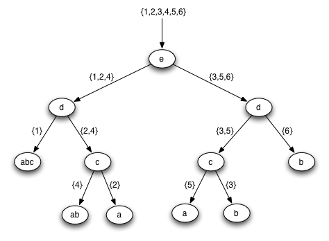
Figure 1: A query plan tree for the example OJ instance

The query plan tree is built recursively as follows. We first arbitrarily order the hyperedges. In the example shown in Figure 1, we have built a tree with the order $e,d,c,b,a$. The root node has universe $V$. We visit these edges one by one in that order.

If every remaining hyperedges contains the universe $V$ then label the node with all remaining hyperedges and stop. In this case the node is a leaf node. Otherwise, consider the next hyperedge in the visiting order above (it is $e$ as we are in the beginning). Label the root with $e$, and create two children of the root $e$. The left child will have universe $V-e$, and the right child has $e$ as its universe. Now, we recursively build the left tree starting from the next hyperedge (i.e. $d$) in the ordering, but only restricting to the smaller universe $\{1,2,4\}$. Similarly, we build the right tree starting from the next hyperedge ($d$) in the ordering, but only restricting to the smaller universe $\{3,5,6\}$.

Let us explain one more level of the tree building process to make things clear. Consider the left tree of the root node $e$. The universe is $\{1,2,4\}$. The root node will be the next hyperedge $d$ in the ordering. But we really work on the restriction of $d$ in the universe $\{1,2,4\}$, which is $d^{\prime}=d\cap\{1,2,4\}=\{2,4\}$. Then, we create two children. The left child has universe $\{1,2,4\}-d^{\prime}=\{1\}$. The right child has universe $d^{\prime}=\{2,4\}$. For the left child, the universe has size $1$ and all three remaining hyperedges $a$, $b$, and $c$ contain $1$, hence we label the left child with $abc$.

By visiting all leaf nodes from left to right and print the attributes in their universes, we obtain something called the total order of all attributes in $V$. In the figure, the total order is $1,4,2,5,3,6$. (In the general case, the total order is slightly more complicated than in this example. See Procedure 4.)

Finally, based on the total order $1,4,2,5,3,6$ just obtained, we build search trees for all relations respecting this ordering. For relation $R_{a}$, the top level of the tree is indexed over attribute $1$, the next two levels are $4$ and $2$, and the last level is indexed over attribute $5$. For $R_{b}$, the order is $1,4,3,6$. For $R_{c}$, the order is $1,2,3$. For $R_{d}$, the order is $4,2,6$. For $R_{e}$, the order is $5,3,6$. It will be clear later that the attribute orders in the search trees have a decisive effect on the overall running time. This is also the step that is responsible for the term $O(n^{2}\sum_{e}N_{e})$ in the overall running time.

Step 1. (This step corresponds to the left most node of the query plan tree.) Compute the join

$$T_{1}=\pi_{\{1\}}(R_{a})\Join\pi_{\{1\}}(R_{b})\Join\pi_{\{1\}}(R_{c})$$ (5)

as follows. This is the join over attributes not in $d$ and $e$. If $|\pi_{\{1\}}(R_{a})|$ is the smallest among $|\pi_{\{1\}}(R_{a})|$, $|\pi_{\{1\}}(R_{b})|$, and $|\pi_{\{1\}}(R_{c})|$, then for each attribute $t_{1}\in\pi_{\{1\}}(R_{a})$, we search the first levels of the search trees for $R_{b}$ and $R_{c}$ to see if $t_{1}$ is in both $\pi_{\{1\}}(R_{b})$ and $\pi_{\{1\}}(R_{b})$. Similarly, if $|\pi_{\{1\}}(R_{b})|$ or $|\pi_{\{1\}}(R_{c})|$ is the smallest then for each $t_{1}\in\pi_{\{1\}}(R_{b})$ (or in $\pi_{\{1\}}(R_{c})$) we search for attribute $t_{1}$ in the other two search trees. As attribute $1$ is in the first level of all three search trees, the join (5) can be computed in time

$$O(|T_{1}|)=O\left(\min\left\{|\pi_{\{1\}}(R_{a})|,|\pi_{\{1\}}(R_{b})|,|\pi_{\{1\}}(R_{c})|\right\}\right).$$

Note that

$$|T_{1}|\leq\min\left\{|\pi_{\{1\}}(R_{a})|,|\pi_{\{1\}}(R_{b})|,|\pi_{\{1\}}(R_{c})|\right\}\leq|\pi_{\{1\}}(R_{a})|^{x_{a}}|\pi_{\{1\}}(R_{b})|^{x_{b}}|\pi_{\{1\}}(R_{c})|^{x_{c}}\leq N_{a}^{x_{a}}N_{b}^{x_{b}}N_{c}^{x_{c}}$$

because $x_{a}+x_{b}+x_{c}\geq 1$. In particular, step 1 can be performed within the run-time budget.

Step 2. (This step corresponds to the node labeled $d$ on the left branch of query plan tree.) Compute the join

$$T_{\{1,2,4\}}=\pi_{\{1,2,4\}}(R_{a})\Join\pi_{\{1,4\}}(R_{b})\Join\pi_{\{1,2\}}(R_{c})\Join\pi_{\{2,4\}}(R_{d})$$

This is a join over all attributes not in $e$.

Since we have already computed the join $T_{1}$ over attribute $1$ of $R_{a}$, $R_{b}$, and $R_{c}$, the relation $T_{\{1,2,4\}}$ can be computed by computing for every $t_{1}\in T_{1}$ the $t_{1}$-section of $T_{\{1,2,4\}}$

$$T_{\{1,2,4\}}[t_{1}]=\underbrace{\pi_{\{2,4\}}(R_{a}[t_{1}])}_{A[t_{1}]}\Join\underbrace{\pi_{\{4\}}(R_{b}[t_{1}])}_{B[t_{1}]}\Join\underbrace{\pi_{\{2\}}(R_{c}[t_{1}])}_{C[t_{1}]}\Join\underbrace{\pi_{\{2,4\}}(R_{d})}_{D}$$

and then $T_{\{1,2,4\}}$ is simply the union of all the $t_{1}$-sections $T_{\{1,2,4\}}[t_{1}]$. The notations $A[t_{1}]$, $B[t_{1}]$, $C[t_{1}]$, and $D$ are defined for the sake of brevity.

Fix $t_{1}\in T_{1}$, we next describe how $T_{\{1,2,4\}}[t_{1}]$ is computed. If $x_{d}\geq 1$ then we go directly to case 2b below. When $x_{d}<1$, define

$$x^{\prime}_{a} = \frac{x_{a}}{1-x_{d}}$$

$$x^{\prime}_{b} = \frac{x_{b}}{1-x_{d}}$$

$$x^{\prime}_{c} = \frac{x_{c}}{1-x_{d}}.$$

Consider the hypergraph graph $H^{\prime}$ which is the graph $H$ restricted to the vertices $2,4$ and edges $a,b,c$. In particular, $H^{\prime}$ has vertex set $\{2,4\}$ and edges $\{2,4\},\{4\},\{2\}$. It is clear that $x^{\prime}_{a}$,$x^{\prime}_{b}$, and $x^{\prime}_{c}$ form a fractional cover solution of $H^{\prime}$ because $\mathbf{x}$ was a fractional cover solution for $H$. Thus, $H^{\prime}$, $\mathbf{x}^{\prime}=(x^{\prime}_{a},x^{\prime}_{b},x^{\prime}_{c})$, and $A[t_{1}]$, $B[t_{1}]$, and $C[t_{1}]$ form an instance of the OJ problem. We will recursively solve this instance if a condition is satisfied.

Case 2a. Suppose

$$|A[t_{1}]|^{x^{\prime}_{a}}|B[t_{1}]|^{x^{\prime}_{b}}|C[t_{1}]|^{x^{\prime}_{c}}\leq|D|$$

then we (recursively) compute the join $A[t_{1}]\Join B[t_{1}]\Join C[t_{1}]$. By induction on the instance $H^{\prime}$, this join can be computed in time

$$O\left(|A[t_{1}]|^{x^{\prime}_{a}}|B[t_{1}]|^{x^{\prime}_{b}}|C[t_{1}]|^{x^{\prime}_{c}}\right).$$

(This induction hypothesis corresponds to the node labeled $c$ on the left branch of the query plan tree.) Here, we crucially use the fact that the search trees for $R_{a}$, $R_{b}$, $R_{c}$ have been built so that the subtrees under the branch $t_{1}$ are precisely the search trees for relations $A[t_{1}],B[t_{1}],C[t_{1}]$ and thus are readily available to compute this join. Now, to get $T_{\{1,2,4\}}[t_{1}]$ we simply check whether every tuple in $A[t_{1}]\Join B[t_{1}]\Join C[t_{1}]$ belongs to $D$.

Case 2b. Suppose either $x_{d}\geq 1$ or

$$|D|\leq|A[t_{1}]|^{x^{\prime}_{a}}|B[t_{1}]|^{x^{\prime}_{b}}|C[t_{1}]|^{x^{\prime}_{c}}$$

then for every tuple $(t_{2},t_{4})$ in $D$ we check whether $(t_{2},t_{4})\in A[t_{1}]$, $t_{4}\in B[t_{1}]$, and $t_{2}\in C[t_{1}]$. The overall running time is $O(|D|)$.

Thus, for a fixed value $t_{1}$, the relation $T_{\{1,2,4\}}[t_{1}]$ can be computed in time

$$O\left(\min\{|A[t_{1}]|^{x^{\prime}_{a}}|B[t_{1}]|^{x^{\prime}_{b}}|C[t_{1}]|^{x^{\prime}_{c}},|D|\}\right).$$

In fact, it is not hard to see that

$$|T_{\{1,2,4\}}[t_{1}]|\leq\min\{|A[t_{1}]|^{x^{\prime}_{a}}|B[t_{1}]|^{x^{\prime}_{b}}|C[t_{1}]|^{x^{\prime}_{c}},|D|\}.$$

This observation will eventually imply the inequality (2) (for this instance), and in the general case leads to the constructive proof of the inequality (2).

Next, note that

$$\min\left\{|A[t_{1}]|^{x^{\prime}_{a}}|B[t_{1}]|^{x^{\prime}_{b}}|C[t_{1}]|^{x^{\prime}_{c}},|D|\right\} \leq \left(|A[t_{1}]|^{x^{\prime}_{a}}|B[t_{1}]|^{x^{\prime}_{b}}|C[t_{1}]|^{x^{\prime}_{c}}\right)^{1-x_{d}}|D|^{x_{d}}$$

$$= |A[t_{1}]|^{x_{a}}|B[t_{1}]|^{x_{b}}|C[t_{1}]|^{x_{c}}|D|^{x_{d}}.$$

If $x_{d}\geq 1$ then the run-time is also in the order of $O(|A[t_{1}]|^{x_{a}}|B[t_{1}]|^{x_{b}}|C[t_{1}]|^{x_{c}}|D|^{x_{d}})$. Consequently, the total running time for step 2 is in the order of

$$\sum_{t_{1}\in T_{1}}|A[t_{1}]|^{x_{a}}|B[t_{1}]|^{x_{b}}|C[t_{1}]|^{x_{c}}|D|^{x_{d}} = |D|^{x_{d}}\sum_{t_{1}\in T_{1}}|A[t_{1}]|^{x_{a}}|B[t_{1}]|^{x_{b}}|C[t_{1}]|^{x_{c}}$$

$$\leq |D|^{x_{d}}\left(\sum_{t_{1}\in T_{1}}|A[t_{1}]|\right)^{x_{a}}\left(\sum_{t_{1}\in T_{1}}|B[t_{1}]|\right)^{x_{b}}\left(\sum_{t_{1}\in T_{1}}|C[t_{1}]|\right)^{x_{c}}$$

$$\leq |D|^{x_{d}}\cdot|\pi_{\{1,2,4\}}(R_{a})|^{x_{a}}\cdot|\pi_{\{1,4\}}(R_{b})|^{x_{b}}\cdot|\pi_{\{1,2\}}(R_{c})|^{x_{c}}$$

$$\leq N_{a}^{x_{a}}N_{b}^{x_{b}}N_{c}^{x_{c}}N_{d}^{x_{d}}.$$

The first inequality follows from generalized Hölder inequality because $x_{a}+x_{b}+x_{c}\geq=1$ and $x_{a},x_{b},x_{c}\geq 0$. The second inequality says that if we sum over the sizes of the $t_{1}$-sections, we get at most the size of the relation. In summary, step $2$ is still within the running time budget.

Step 3. Compute the final join over all attributes

$$T_{\{1,2,3,4,5,6\}}=R_{a}\Join R_{b}\Join R_{c}\Join R_{d}\Join R_{e}.$$

Since we have already computed the join $T_{\{1,2,4\}}$ over attributes $1,2,4$ of $R_{a}$, $R_{b}$, $R_{c}$, and $R_{d}$, the relation $T_{\{1,2,3,4,5,6\}}$ can be computed by computing for every $(t_{1},t_{2},t_{4})\in T_{\{1,2,4\}}$ the join

$$T_{\{1,2,3,4,5,6\}}[t_{1},t_{2},t_{4}]=\underbrace{\pi_{\{5\}}(R_{a}[t_{1},t_{2},t_{4}])}_{A}\Join\underbrace{\pi_{\{3,6\}}(R_{b}[t_{1},t_{4}])}_{B}\Join\underbrace{\pi_{\{3\}}(R_{c}[t_{1},t_{2}])}_{C}\Join\underbrace{\pi_{\{6\}}(R_{d}[t_{2},t_{4}])}_{D}\Join\underbrace{R_{e}}_{E},$$

and return the union of these joins over all tuples $(t_{1},t_{2},t_{4})\in T_{\{1,2,4\}}$. Again, the notations $A$, $B$, $C$, $D$, $E$ are introduced to for the sake of brevity. Note, however, that they are different from the $A$, $B$, $C$, $D$ from case 2. This step illustrates the third ingredient of the algorithm’s analysis.

Fix $(t_{1},t_{2},t_{4})\in T_{\{1,2,4\}}$. If $x_{e}\geq 1$ then we jump to case 3b; otherwise, define

$$x^{\prime\prime}_{a} = \frac{x_{a}}{1-x_{e}}$$

$$x^{\prime\prime}_{b} = \frac{x_{b}}{1-x_{e}}$$

$$x^{\prime\prime}_{c} = \frac{x_{c}}{1-x_{e}}$$

$$x^{\prime\prime}_{d} = \frac{x_{d}}{1-x_{e}}.$$

Then define a hypergraph $H^{\prime\prime}$ on the attributes $\{3,5,6\}$ and the restrictions of $a$, $b$, $c$, $d$ on these attributes. Clearly the vector $\mathbf{x}^{\prime\prime}$ is a fractional cover for this instance.

Case 3a. Suppose $x_{e}\geq 1$ or

$$|A|^{x^{\prime\prime}_{a}}|B|^{x^{\prime\prime}_{b}}|C|^{x^{\prime\prime}_{c}}|D|^{x^{\prime\prime}_{d}}\leq|E|.$$

By applying the induction hypothesis on the $H^{\prime\prime}$ instance we can compute the join $A\Join B\Join C\Join D$ in time $O\left(|A|^{x^{\prime\prime}_{a}}|B|^{x^{\prime\prime}_{b}}|C|^{x^{\prime\prime}_{c}}|D|^{x^{\prime\prime}_{d}}\right)$. (The induction hypothesis corresponds to the node labeled $d$ on right branch of the query plan tree.) Again, because the search trees for all relations have been built in such a way that the search trees for $A$, $B$, $C$, $D$ are already present on $t_{1},t_{2},t_{4}$-branches of the trees for $R_{a},R_{b},R_{c}$, and $R_{d}$, there is no extra time spent on indexing for computing this join. Then, for every tuple $\mathbf{t}_{\{3,5,6\}}$ in the join we check (the search tree for) $E$ to see if the tuple belongs to $E$.

Case 3b. Suppose

$$|E|\leq|A|^{x^{\prime\prime}_{a}}|B|^{x^{\prime\prime}_{b}}|C|^{x^{\prime\prime}_{c}}|D|^{x^{\prime\prime}_{d}}.$$

Then, for each tuple $\mathbf{t}_{\{3,5,6\}}=(t_{3},t_{5},t_{6})\in E$ we check to see whether $t_{5}\in A,(t_{3},t_{6})\in B,t_{3}\in C$, and $t_{6}\in D$.

Either way, for a fix tuple $(t_{1},t_{2},t_{4})\in T_{\{1,2,4\}}$ the running time is

$$\tilde{O}\left(\min\left\{|A|^{x^{\prime\prime}_{a}}|B|^{x^{\prime\prime}_{b}}|C|^{x^{\prime\prime}_{c}}|D|^{x^{\prime\prime}_{d}},|E|\right\}\right).$$

Now, we apply the same trick as in case 2:

$$\min\left\{|A|^{x^{\prime\prime}_{a}}|B|^{x^{\prime\prime}_{b}}|C|^{x^{\prime\prime}_{c}}|D|^{x^{\prime\prime}_{d}},|E|\right\} \leq \left(|A|^{x^{\prime\prime}_{a}}|B|^{x^{\prime\prime}_{b}}|C|^{x^{\prime\prime}_{c}}|D|^{x^{\prime\prime}_{d}}\right)^{1-x_{e}}|E|^{x_{e}}$$

$$= |A|^{x_{a}}|B|^{x_{b}}|C|^{x_{c}}|D|^{x_{d}}|E|^{x_{e}}$$

$$\leq |R_{a}[t_{1},t_{2},t_{4}]|^{x_{a}}|R_{b}[t_{1},t_{4}]|^{x_{b}}|R_{c}[t_{1},t_{2}]|^{x_{c}}|R_{d}[t_{2},t_{4}]|^{x_{d}}|R_{e}|^{x_{e}}.$$

Hence, the total running time for step $3$ is in the order of

$$\sum_{(t_{1},t_{2},t_{4})\in T_{\{1,2,4\}}}|R_{a}[t_{1},t_{2},t_{4}]|^{x_{a}}|R_{b}[t_{1},t_{4}]|^{x_{b}}|R_{c}[t_{1},t_{2}]|^{x_{c}}|R_{d}[t_{2},t_{4}]|^{x_{d}}|R_{e}|^{x_{e}}$$

$$= |R_{e}|^{x_{e}}\sum_{t_{1}}\sum_{t_{2}}\sum_{t_{4}}|R_{a}[t_{1},t_{2},t_{4}]|^{x_{a}}|R_{b}[t_{1},t_{4}]|^{x_{b}}|R_{c}[t_{1},t_{2}]|^{x_{c}}|R_{d}[t_{2},t_{4}]|^{x_{d}}$$

where the first sum is over $t_{1}\in\pi_{\{1\}}(T_{\{1,2,4\}})$, the second sum is over $t_{2}$ such that $(t_{1},t_{2})\in\pi_{\{1,2\}}(T_{\{1,2,4\}})$, and the third sum is over $t_{4}$ such that $(t_{1},t_{2},t_{4})\in T_{\{1,2,4\}}$. We apply Hölder inequality several times to “unroll” the sums. Note that we crucially use the fact that $\mathbf{x}$ is a fractional cover solution ($\mathbf{M}\mathbf{x}\geq\mathbf{1}$) to apply Hölder’s inequality.

$$|R_{e}|^{x_{e}}\sum_{t_{1}}\sum_{t_{2}}\sum_{t_{4}}|R_{a}[t_{1},t_{2},t_{4}]|^{x_{a}}|R_{b}[t_{1},t_{4}]|^{x_{b}}|R_{c}[t_{1},t_{2}]|^{x_{c}}|R_{d}[t_{2},t_{4}]|^{x_{d}}$$

$$= |R_{e}|^{x_{e}}\sum_{t_{1}}\sum_{t_{2}}|R_{c}[t_{1},t_{2}]|^{x_{c}}\sum_{t_{4}}|R_{a}[t_{1},t_{2},t_{4}]|^{x_{a}}|R_{b}[t_{1},t_{4}]|^{x_{b}}|R_{d}[t_{2},t_{4}]|^{x_{d}}$$

$$\leq |R_{e}|^{x_{e}}\sum_{t_{1}}\sum_{t_{2}}|R_{c}[t_{1},t_{2}]|^{x_{c}}\left(\sum_{t_{4}}|R_{a}[t_{1},t_{2},t_{4}]|\right)^{x_{a}}\left(\sum_{t_{4}}|R_{b}[t_{1},t_{4}]|\right)^{x_{b}}\left(\sum_{t_{4}}|R_{d}[t_{2},t_{4}]|\right)^{x_{d}}$$

$$\leq |R_{e}|^{x_{e}}\sum_{t_{1}}\sum_{t_{2}}|R_{c}[t_{1},t_{2}]|^{x_{c}}|R_{a}[t_{1},t_{2}]|^{x_{a}}|R_{b}[t_{1}]|^{x_{b}}|R_{d}[t_{2}]|^{x_{d}}$$

$$= |R_{e}|^{x_{e}}\sum_{t_{1}}|R_{b}[t_{1}]|^{x_{b}}\sum_{t_{2}}|R_{c}[t_{1},t_{2}]|^{x_{c}}|R_{a}[t_{1},t_{2}]|^{x_{a}}|R_{d}[t_{2}]|^{x_{d}}$$

$$\leq |R_{e}|^{x_{e}}\sum_{t_{1}}|R_{b}[t_{1}]|^{x_{b}}\left(\sum_{t_{2}}|R_{c}[t_{1},t_{2}]|\right)^{x_{c}}\left(\sum_{t_{2}}|R_{a}[t_{1},t_{2}]|\right)^{x_{a}}\left(\sum_{t_{2}}|R_{d}[t_{2}]|\right)^{x_{d}}$$

$$\leq |R_{e}|^{x_{e}}\sum_{t_{1}}|R_{b}[t_{1}]|^{x_{b}}|R_{c}[t_{1}]|^{x_{c}}|R_{a}[t_{1}]|^{x_{a}}|R_{d}|^{x_{d}}$$

$$= |R_{e}|^{x_{e}}|R_{d}|^{x_{d}}\sum_{t_{1}}|R_{b}[t_{1}]|^{x_{b}}|R_{c}[t_{1}]|^{x_{c}}|R_{a}[t_{1}]|^{x_{a}}$$

$$\leq |R_{e}|^{x_{e}}|R_{d}|^{x_{d}}\left(\sum_{t_{1}}|R_{b}[t_{1}]|\right)^{x_{b}}\left(\sum_{t_{1}}|R_{c}[t_{1}]|\right)^{x_{c}}\left(\sum_{t_{1}}|R_{a}[t_{1}]|\right)^{x_{a}}$$

$$\leq |R_{e}|^{x_{e}}|R_{d}|^{x_{d}}|R_{b}|^{x_{b}}|R_{c}|^{x_{c}}|R_{a}|^{x_{a}}.$$

5.3 Rigorous description and analysis of the algorithm

Algorithm 2 computes the join of $m$ given relations. Beside the relations, the input to the algorithm consists of the hypergraph $H=(V,E)$ with $|V|=n$, $|E|=m$, and a point $\mathbf{x}=(x_{e})_{e\in E}$ in the fractional cover polytope

$$\sum_{v\in e}x_{e} \geq 1,\ \text{for any $v\in V$}$$

$$x_{e} \geq 0,\text{for any $e\in E$}.$$

1. We first build a query plan tree. The query plan tree serves two purposes: (a) it captures the structure of the recursions in the algorithm where each node of the tree roughly corresponds to a sub-problem, (b) it gives a total order of all the attributes based on which we can pre-build search trees for all the relations in the next step.

2. From the query plan tree, we construct a total order of all attributes in $V$. Then, for each relation $R_{e}$ we construct a search tree for $R_{e}$ based on the relative order of $R_{e}$’s attributes imposed by the total order.

3. We traverse the query plan tree and solve some of the sub-problems and combine the solutions to form the final answer. It is important to note that not all sub-problems corresponding to nodes in the query plan trees will be solved. We decide whether to solve a sub-problem based on a “size check.” Intuitively, if the sub-problem is estimated to have a large output size we will try to not solve it.

Algorithm 2 Computing the join $\Join_{e\in E}R_{e}$

0:  Hypergraph $H=(V,E)$, $|V|=n$, $|E|=m$

0:  Fractional cover solution $\mathbf{x}=(x_{e})_{e\in E}$

0:  Relations $R_{e},e\in E$

1:  Compute the query plan tree $\mathcal{T}$, let $u$ be $\mathcal{T}$’s root node

2:  Compute a total order of attributes

3:  Compute a collection of hash indices for all relations

4:  return  Recursive-Join$(u,\mathbf{x},\text{\sc nil})$

We repeat some of the terminologies already defined so that this section is relatively self-contained. For each tuple $\mathbf{t}$ on attribute set $A$, we will write $\mathbf{t}$ as $\mathbf{t}_{A}$ to signify the fact that the tuple is on the attribute set $A$: $\mathbf{t}_{A}=(t_{a})_{a\in A}$. Consider any relation $R$ with attribute set $S$. Let $A\subset S$ and $\mathbf{t}_{A}$ be a fixed tuple. Then $R[\mathbf{t}_{A}]$ denotes the “$\mathbf{t}_{A}$-section” of $R$, which is a relation on $S-A$ consisting of all tuples $\mathbf{t}_{S-A}$ such that $(\mathbf{t}_{A},\mathbf{t}_{S-A})\in R$. In particular, $R[\mathbf{t}_{\emptyset}]=R$. Let $\pi_{A}(R)$ denote the projection of $R$ down to attributes in $A$.

5.3.1 Step (1): Building the query plan tree

1:  Fix an arbitrary order $e_{1},e_{2},\dots,e_{m}$ of all the hyperedges in $E$.

2:  $\mathcal{T}\leftarrow$ build-tree$(V,m)$

build-tree$(U,k)$

1:  if $e_{i}\cap U=\emptyset,\forall i\in[k]$ then

2:        return  nil

3:  Create a node $u$ with $\text{\sc label}(u)\leftarrow k$ and $\text{\sc univ}(u)=U$

4:  if $k>1$ and $\exists i\in[k]$ such that $U\not\subseteq e_{i}$ then

5:        $\text{\sc lc}(u)\leftarrow$ build-tree$(U\setminus e_{k},k-1)$

6:        $\text{\sc rc}(u)\leftarrow$ build-tree$(U\cap e_{k},k-1)$

7:  return  $u$

Algorithm 3 Constructing the query plan tree $\mathcal{T}$

Very roughly, each node $x$ and the sub-tree below it forms the “skeleton” of a sub-problem. There will be many sub-problems that correspond to each skeleton. The value $\text{\sc label}(x)$ points to an “anchor” relation for the sub-problem and $\text{\sc univ}(x)$ is the set of attributes that the sub-problem is joining on. The anchor relation divides the universe $\text{\sc univ}(x)$ into two parts to further sub-divide the recursion structure. Fix an arbitrary order $e_{1},e_{2},\dots,e_{m}$ of all the hyperedges in $E$. For notational convenience, for any $k\in[m]$ define $E_{k}=\{e_{1},\dots,e_{k}\}$. The query plan tree $\mathcal{T}$ is a binary tree with the following associated information:

• Labels. Each node of $\mathcal{T}$ has a “label” $\text{\sc label}(u)$ which is an integer $k\in[m]$.

• Universes. Each node $u$ of $\mathcal{T}$ has a “universe” $\text{\sc univ}(u)$ which is a non-empty subset of attributes: $\text{\sc univ}(u)\subseteq V$.

• Each internal node $u$ of $\mathcal{T}$ has a left child $\text{\sc lc}(u)$ or a right child $\text{\sc rc}(u)$ or both. If a child does not exist then the child pointer points to nil.

Algorithm 3 builds the query plan tree $\mathcal{T}$. Very roughly, each node $x$ and the sub-tree below it forms the “skeleton” of a sub-problem. There will be many sub-problems that correspond to each skeleton. The value $\text{\sc label}(x)$ points to an “anchor” relation for the sub-problem and $\text{\sc univ}(x)$ is the set of attributes that the sub-problem is joining on. The anchor relation divides the universe $\text{\sc univ}(x)$ into two parts to further sub-divide the recursion structure.

Note that line 5 and 6 will not be executed if $U\subseteq e_{i},\forall i\in[k]$, in which case $u$ is a leaf node. When $u$ is not a leaf node, if $U\subseteq e_{k}$ then $u$ will not have a left child ($\text{\sc lc}(u)=\text{\sc nil}$). The running time for this pre-processing step is $O(m^{2}n)$.

Figure 2 shows a query plan tree produced by Algorithm 3 on an example query.

$\displaystyle q$ $\displaystyle=$ $\displaystyle R_{1}(A_{1},A_{2},A_{4},A_{5})$ $\displaystyle\Join$ $\displaystyle R_{2}(A_{1},A_{3},A_{4},A_{6})$ $\displaystyle\Join$ $\displaystyle R_{3}(A_{1},A_{2},A_{3})$ $\displaystyle\Join$ $\displaystyle R_{4}(A_{2},A_{4},A_{6})$ $\displaystyle\Join$ $\displaystyle R_{5}(A_{3},A_{5},A_{6})$

Figure 2: (a) A query $q$ and (b) a sample QP tree for $q$.

5.3.2 Step (2): Computing a total order of the attributes and building the search trees

From the query plan tree $\mathcal{T}$, Procedure 4 constructs a total order of all the attributes in $V$. We will call this ordering the total order of $V$. It is not hard to see that the total order satisfies the following proposition.

Proposition 5.5.

The total order computed in Algorithm 4 satisfies the following properties

• For every node $u$ in the query plan tree $\mathcal{T}$, all members of $\text{\sc univ}(u)$ are consecutive in the total order

• For every internal node $u$, if $\text{\sc label}(u)=k$ and $S$ is the set of all attributes preceding $\text{\sc univ}(u)$ in the total order, then $S\cup\text{\sc univ}(\text{\sc lc}(u))=S\cup(U\setminus e_{k})$ is precisely the set of all attributes preceding $\text{\sc univ}(\text{\sc rc}(u))=e_{k}\cap U$ in the total order.

Algorithm 4 Computing a total order of attributes in $V$

1:  Let $\mathcal{T}$ be the query plan tree with root node $u$, where $\text{\sc univ}(u)=V$

2:  print-attribs$(u)$

print-attribs$(u)$

1:  if $u$ is a leaf node of $\mathcal{T}$ then

2:        print  all attributes in $\text{\sc univ}(u)$ in an arbitrary order

3:  else if $\text{\sc lc}(u)=\text{\sc nil}$ then

4:        print-attribs$(\text{\sc rc}(u))$

5:  else if $\text{\sc rc}(u)=\text{\sc nil}$ then

6:        print-attribs$(\text{\sc lc}(u))$

7:        print  all attributes in $\text{\sc univ}(u)\setminus\text{\sc univ}(\text{\sc lc}(u))$ in an arbitrary order

8:  else

9:        print-attribs$(\text{\sc lc}(u))$

10:        print-attribs$(\text{\sc rc}(u))$

For each relation $R_{e}$, $e\in E$, we order all attributes in $R_{e}$ such that the internal order of attributes in $R_{e}$ is consistent with the total order of all attributes computed by Algorithm 4. More concretely, suppose $R_{e}$ has $k$ attributes ordered $a_{1},\dots,a_{k}$, then $a_{i}$ must come before $a_{i+1}$ in the total order, for all $1\leq i\leq k-1$. Then, we build a search tree (or any indexing data structure) for every relation $R_{e}$ using the internal order of $R_{e}$’s attributes: $a_{1}$ indexes level $1$ of the tree, $a_{2}$ indexes the next level, $\dots$, $a_{k}$ indexes the last level of the tree. The search tree for relation $R_{e}$ is constructed to satisfy the following three properties. Let $i$ and $j$ be arbitrary integers such that $1\leq i\leq j\leq k$. Let $\mathbf{t}_{\{a_{1},\dots,a_{i}\}}=(t_{a_{1}},\dots,t_{a_{i}})$ be an arbitrary tuple on the attributes $\{a_{1},\dots,a_{i}\}$.

• We can decide whether $\mathbf{t}_{\{a_{1},\dots,a_{i}\}}\in\pi_{\{a_{1},\dots,a_{i}\}}(R_{e})$ in $O(i)$-time (by “stepping down” the tree along the $t_{a_{1}},\dots,t_{a_{i}}$ path).

• We can query the size $|\pi_{\{a_{i+1},\dots,a_{j}\}}(R_{e}[\mathbf{t}_{\{a_{1},\dots,a_{i}\}}])|$ in $O(i)$ time.

• We can list all tuples in the set $\pi_{\{a_{i+1},\dots,a_{j}\}}(R_{e}[\mathbf{t}_{\{a_{1},\dots,a_{i}\}}])$ in time linear in the output size if the output is not empty.

The total running time for building all the search trees is $O(n^{2}\sum_{e}N_{e})$.

5.3.3 Step (3): Computing the join

Procedure 5 Recursive-Join$(u,\mathbf{y},\mathbf{t}_{S})$

1:  Let $U=\text{\sc univ}(u)$, $k=\text{\sc label}(u)$

2:  $\text{Ret}\leftarrow\emptyset$ // Ret is the returned tuple set

3:  if $u$ is a leaf node of $\mathcal{T}$ then // note that $U\subseteq e_{i},\forall i\leq k$

4:        $j\leftarrow\mathop{\text{argmin}}_{i\in[k]}\left\{|\pi_{U}(R_{e_{i}}[\mathbf{t}_{S\cap e_{i}}])|\right\}$

5:        // By convention, $R_{e}[\text{\sc nil}]=R_{e}$ and $R_{e}[\mathbf{t}_{\emptyset}]=R_{e}$

6:        for each tuple $\mathbf{t}_{U}\in\pi_{U}(R_{e_{j}}[\mathbf{t}_{S\cap e_{j}}])$ do

7:              if $\mathbf{t}_{U}\in\pi_{U}(R_{e_{i}}[\mathbf{t}_{S\cap e_{i}}]),\text{ for all }i\in[k]\setminus\{j\}$ then

8:                    $\text{Ret}\leftarrow\text{Ret}\cup\{(\mathbf{t}_{S},\mathbf{t}_{U})\}$

9:        return  Ret

10:  if $\text{\sc lc}(u)=\text{\sc nil}$ then // $u$ is not a leaf node of $\mathcal{T}$

11:        $L\leftarrow\{\mathbf{t}_{S}\}$

12:        // note that $L\neq\emptyset$ and $\mathbf{t}_{S}$ could be nil (when $S=\emptyset$)

13:  else

14:        $L\leftarrow$ Recursive-Join$(\text{\sc lc}(u),(y_{1},\dots,y_{k-1}),\mathbf{t}_{S})$

15:  $W\leftarrow U\setminus e_{k}$, $W^{-}\leftarrow e_{k}\cap U$

16:  if $W^{-}=\emptyset$ then

17:        return  $L$

18:  for each tuple $\mathbf{t}_{S\cup W}=(\mathbf{t}_{S},\mathbf{t}_{W})\in L$ do

19:        if $y_{e_{k}}\geq 1$ then

20:              go to line 27

21:        if $\displaystyle{\left(\prod_{i=1}^{k-1}|\pi_{e_{i}\cap W^{-}}(R_{e_{i}}[\mathbf{t}_{(S\cup W)\cap e_{i}}])|^{\frac{y_{e_{i}}}{1-y_{e_{k}}}}<|\pi_{W^{-}}(R_{e_{k}}[\mathbf{t}_{S\cap e_{k}}])|\right)}$ then

22:              $Z\leftarrow$ Recursive-Join$\left(\text{\sc rc}(u),\left(\frac{y_{e_{i}}}{1-y_{e_{k}}}\right)_{i=1}^{k-1},\mathbf{t}_{S\cup W}\right)$

23:              for each tuple $(\mathbf{t}_{S},\mathbf{t}_{W},\mathbf{t}_{W^{-}})\in Z$ do

24:                    if $\mathbf{t}_{W^{-}}\in\pi_{W^{-}}(R_{e_{k}}[\mathbf{t}_{S\cap e_{k}}])$ then

25:                          $\text{Ret}\leftarrow\text{Ret}\cup\{(\mathbf{t}_{S},\mathbf{t}_{W},\mathbf{t}_{W^{-}})\}$

26:        else

27:              for each tuple $\mathbf{t}_{W^{-}}\in\pi_{W^{-}}(R_{e_{k}}[\mathbf{t}_{S\cap e_{k}}])$ do

28:                    if $\mathbf{t}_{e_{i}\cap W^{-}}\in\pi_{e_{i}\cap W^{-}}(R_{e_{i}}[\mathbf{t}_{(S\cup W)\cap e_{i}}])$ for all $e_{i}$ such that $i<k$ and $e_{i}\cap W^{-}\neq\emptyset$ then

29:                          $\text{Ret}\leftarrow\text{Ret}\cup\{(\mathbf{t}_{S},\mathbf{t}_{W},\mathbf{t}_{W^{-}})\}$

30:  return  Ret

At the heart of Algorithm 2 is a recursive procedure called Recursive-Join (Procedure 5) which takes three arguments:

• a node $u$ from the query plan tree $\mathcal{T}$ whose label is $k$ for some $k\in[m]$.

• a fractional cover solution $\mathbf{y}_{E_{k}}=(y_{e_{1}},\dots,y_{e_{k}})$ of the hypergraph $(\text{\sc univ}(u),E_{k})$. Here, we only take the restrictions of hyperedges of $E_{k}$ onto the universe $\text{\sc univ}(u)$. Specifically,

  $$\sum_{e\in E_{k}:i\in e}y_{e} \geq 1,\ \text{for any $i\in\text{\sc univ}(u)$}$$

  $$y_{e} \geq 0,\text{for any $e\in E_{k}$}$$

• a tuple $\mathbf{t}_{S}=(t_{i})_{i\in S}$ where $S$ is the set of all attributes in $V$ which precede $\text{\sc univ}(u)$ in the total order. (Due to property (TO1) of Proposition 5.5, the set $S$ is well-defined.) If there is no attribute preceding $\text{\sc univ}(u)$ then this argument is nil. In particular, the argument is nil if $u$ is a node along the left path of QP-tree $\mathcal{T}$ from the root down to the left-most leaf.

Throughout this section, we denote the final output by $J$ which is defined to be $J=\Join_{e\in E}R_{e}$. The goal of Recursive-Join is to compute a superset of the relation $\{\mathbf{t}_{S}\}\times\pi_{\text{\sc univ}(u)}(J[\mathbf{t}_{S}])$, i.e., a superset of the output tuples that start with $\mathbf{t}_{S}$ on the attributes $S\cup\text{\sc univ}(u)$. This intermediate output is analogous to the set $C$ in Algorithm 1 for LW instances. A second similarity Algorithm 1 is that our algorithm makes a choice per tuple based on the output’s estimated size.

Theorem 5.1 is a special case of the following lemma where we set $u$ to be the root of the QP-tree $\mathcal{T}$, $\mathbf{y}=\mathbf{x}$, and $S=\emptyset$ ($\mathbf{t}_{S}=\text{\sc nil}$). Finally, we observe that we need only $O(n^{2})$ number of hash indices per input relation, which completes the proof.

Lemma 5.6.

Consider a call Recursive-Join$(u,\mathbf{y},\mathbf{t}_{S})$ to Procedure 5. Let $k=\text{\sc label}(u)$ and $U=\text{\sc univ}(u)$. Then,

• The procedure outputs a relation Ret on attributes $S\cup U$ with at most the following number of tuples

  $$B(u,\mathbf{y},\mathbf{t}_{S}):=\prod_{i=1}^{k}|\pi_{U\cap e_{i}}(R_{e_{i}}[\mathbf{t}_{S\cap e_{i}}])|^{y_{i}}.$$

  (For the sake of presentation, we agree on the convention that when $U\cap e_{i}=\emptyset$ we set $|\pi_{U\cap e_{i}}(R_{e_{i}}[\mathbf{t}_{S\cap e_{i}}])|=1$ so that the factor does not contribute anything to the product.)

• Furthermore, the procedure runs in time $O(mn\cdot B(u,\mathbf{y},\mathbf{t}_{S}))$.

Proof.

We prove both $(a)$ and $(b)$ by induction on the height of the subtree of $\mathcal{T}$ rooted at $u$. The proof will also explain in “plain” English the algorithm presented in Procedure 5. The procedure tries to compute the join

$$\{\mathbf{t}_{S}\}\times\left(\Join_{i=1}^{k}\pi_{U\cap e_{i}}(R_{e_{i}}[\mathbf{t}_{S\cap e_{i}}])\right).$$

Roughly speaking, it is computing the join of all the sections $R_{e_{i}}[\mathbf{t}_{S\cap e_{i}}]$ inside the universe $U$.

Base case. The height of the sub-tree rooted at $u$ is zero, i.e. $u$ is a leaf node. In this case, lines 4-9 of Procedure 5 is executed. When $u$ is a leaf node, $U\subseteq e_{i},\forall i\in[k]$ and thus $U=U\cap e_{i},\forall i\in[k]$. Since $\mathbf{y}$ is a fractional cover solution to the hypergraph instance $(U,E_{k})$, we know $\sum_{i=1}^{k}y_{i}\geq 1$. The join has size at most

$$\min_{i\in[k]}\left\{|\pi_{U}(R_{e_{i}}[\mathbf{t}_{S\cap e_{i}}])|\right\}\leq\prod_{i=1}^{k}|\pi_{U\cap e_{i}}(R_{e_{i}}[\mathbf{t}_{S\cap e_{i}}])|^{y_{i}}=B(u,\mathbf{y},\mathbf{t}_{S}).$$

To compute the join, we go over each tuple of the smallest-sized section-projection $\pi_{U}(R_{e_{j}}[\mathbf{t}_{S\cap e_{j}}])$ and check to see if the tuple belongs to all the other section-projections. There are at most $k$ other sections, and due to property (ST1) each check takes time $O(n)$. Hence, the total time spent is $O(mn\cdot B(u,\mathbf{y},\mathbf{t}_{S}))$.

Inductive step. Now, consider the case when $u$ is not a leaf node.

If $\text{\sc lc}(u)=\text{\sc nil}$ which means $U\subseteq e_{k}$ then there is no attribute in $U\setminus e_{k}$ to join over (line 11). Otherwise, we first recursively call the “left sub-problem” (Line 14) and store the result in $L$. Note that the attribute set of $L$ is $S\cup W=S\cup(U\setminus e_{k})$. We need to verify that the arguments we gave to this recursive call are legitimate. It should be obvious that $k-1=\text{\sc label}(\text{\sc lc}(u))$. Since $\mathbf{y}=(y_{1},\dots,y_{k})$ is a fractional cover of the $(U,E_{k})$ hypergraph, $\mathbf{y}^{\prime}=(y_{1},\dots,y_{k-1})$ is a fractional cover of the $(U\setminus e_{k},E_{k-1})$ hypergraph. And, $\text{\sc univ}(\text{\sc lc}(u))=U\setminus e_{k}$. Finally, due to property (TO2) $S$ is precisely the set of attributes preceding $\text{\sc univ}(\text{\sc lc}(u))$ in the total order. From the induction hypothesis, the recursive call on line 14 takes time

$$O(mn\cdot B(\text{\sc lc}(u),\mathbf{y}^{\prime},\mathbf{t}_{S}))=O\left(mn\prod_{i=1}^{k-1}|\pi_{W\cap e_{i}}(R_{e_{i}}[\mathbf{t}_{S\cap e_{i}}])|^{y_{i}}\right).$$

Furthermore, the number of tuples in $L$ is at most $B(\text{\sc lc}(u),\mathbf{y}^{\prime},\mathbf{t}_{S})=\prod_{i=1}^{k-1}|\pi_{W\cap e_{i}}(R_{e_{i}}[\mathbf{t}_{S\cap e_{i}}])|^{y_{i}}$.

If $W^{-}=\emptyset$ then $L$ is returned and we are done because in this case $B(\text{\sc lc}(u),\mathbf{y}^{\prime},\mathbf{t}_{S})\leq B(u,\mathbf{y},\mathbf{t}_{S})$.

Consider the for loop from line 18 to line 29. We execute the for loop for each tuple $\mathbf{t}_{S\cup W}=(\mathbf{t}_{S},\mathbf{t}_{W})\in L$. If $L=\emptyset$ then the output is empty and we are done. If $L=\{\mathbf{t}_{S}\}$ then this for-loop is executed only once. This is the case if the assignment in line 11 was performed, which means $U\subseteq e_{k}$ and thus $W=\emptyset$. We do not have to analyze this case separately as it is subsumed by the general case that $L\neq\emptyset$.

Note that if $y_{e_{k}}\geq 1$ then we go directly to case b below (corresponding to line 27).

Case a. Consider the case when $y_{e_{k}}<1$ and

$$\prod_{i=1}^{k-1}|\pi_{e_{i}\cap W^{-}}(R_{e_{i}}[\mathbf{t}_{(S\cup W)\cap e_{i}}])|^{\frac{y_{e_{i}}}{1-y_{e_{k}}}}<|\pi_{W^{-}}(R_{e_{k}}[\mathbf{t}_{S\cap e_{k}}])|.$$

In this case we first recursively solve the sub-problem

$$Z=\text{\sc Recursive-Join}\left(\text{\sc rc}(u),\left(\frac{y_{e_{i}}}{1-y_{e_{k}}}\right)_{i=1}^{k-1},\mathbf{t}_{S\cup W}\right).$$

We need to make sure that the arguments are legitimate. Note that $\text{\sc univ}(\text{\sc rc}(u))=W^{-}$, and that $y_{e_{k}}<1$. The sub-problem is on the hypergraph $(W^{-},E_{k-1})$. For any $v\in W^{-}=U\cap e_{k}$, because $\mathbf{y}$ is a fractional cover of the $(U,E_{k})$ hypergraph,

$$1\leq\sum_{i\in[k]\ :\ v\in e_{i}}y_{e_{i}}=y_{e_{k}}+\sum_{i\in[k-1]\ :\ v\in e_{i}}y_{e_{i}}.$$

Hence,

$$1\leq\sum_{i\in[k-1]\ :\ v\in e_{i}}\frac{y_{e_{i}}}{1-y_{e_{k}}},$$

which confirms that the solution $\left(\frac{y_{e_{i}}}{1-y_{e_{k}}}\right)_{i=1}^{k-1}$ is a fractional cover for the hypergraph $(W^{-},E_{k-1})$. Finally, by property (TO2) the attributes $S\cup W$ are precisely the attributes preceding $W^{-}$ in the total order.

After solving the sub-problem we obtain a tuple set $Z$ over the attributes $S\cup W\cup W^{-}=S\cup U$. By the induction hypothesis the time it takes to solve the sub-problem is

$$O\left(mn\prod_{i=1}^{k-1}|\pi_{e_{i}\cap W^{-}}(R_{e_{i}}[\mathbf{t}_{(S\cup W)\cap e_{i}}])|^{\frac{y_{e_{i}}}{1-y_{e_{k}}}}\right)$$

and the number of tuples in $Z$ is bounded by

$$\prod_{i=1}^{k-1}|\pi_{e_{i}\cap W^{-}}(R_{e_{i}}[\mathbf{t}_{(S\cup W)\cap e_{i}}])|^{\frac{y_{e_{i}}}{1-y_{e_{k}}}}.$$

Then, for each tuple in $Z$ we perform the check on line 24. Hence, the overall running time in this case is still $O\left(mn\prod_{i=1}^{k-1}|\pi_{e_{i}\cap W^{-}}(R_{e_{i}}[\mathbf{t}_{(S\cup W)\cap e_{i}}])|^{\frac{y_{e_{i}}}{1-y_{e_{k}}}}\right)$

Case b. Consider the case when either $y_{e_{k}}\geq 1$ or

$$\prod_{i=1}^{k-1}|\pi_{e_{i}\cap W^{-}}(R_{e_{i}}[\mathbf{t}_{(S\cup W)\cap e_{i}}])|^{\frac{y_{e_{i}}}{1-y_{e_{k}}}}\geq|\pi_{W^{-}}(R_{e_{k}}[\mathbf{t}_{S\cap e_{k}}])|.$$

In this case, we execute lines 27 to 29. The number of tuples output is at most $|\pi_{W^{-}}(R_{e_{k}}[\mathbf{t}_{S\cap e_{k}}])|$ and the running time is $O(mn|\pi_{W^{-}}(R_{e_{k}}[\mathbf{t}_{S\cap e_{k}}])|)$.

Overall, for both (case a) and (case b) the number of tuples output is bounded by

$$T=\begin{cases}\min\left\{\prod_{i=1}^{k-1}|\pi_{e_{i}\cap W^{-}}(R_{e_{i}}[\mathbf{t}_{(S\cup W)\cap e_{i}}])|^{\frac{y_{e_{i}}}{1-y_{e_{k}}}},|\pi_{W^{-}}(R_{e_{k}}[\mathbf{t}_{S\cap e_{k}}])|\right\}&y_{e_{k}}<1\\ |\pi_{W^{-}}(R_{e_{k}}[\mathbf{t}_{S\cap e_{k}}])|&\text{otherwise}\end{cases}$$

and the running time is in the order of $O(mnT)$. We bound $T$ next. When $y_{e_{k}}<1$ we have

$$T \leq \min\left\{\prod_{i=1}^{k-1}|\pi_{e_{i}\cap W^{-}}(R_{e_{i}}[\mathbf{t}_{(S\cup W)\cap e_{i}}])|^{\frac{y_{e_{i}}}{1-y_{e_{k}}}},|\pi_{W^{-}}(R_{e_{k}}[\mathbf{t}_{S\cap e_{k}}])|\right\}$$

$$\leq \left(\prod_{i=1}^{k-1}|\pi_{e_{i}\cap W^{-}}(R_{e_{i}}[\mathbf{t}_{(S\cup W)\cap e_{i}}])|^{\frac{y_{e_{i}}}{1-y_{e_{k}}}}\right)^{1-y_{e_{k}}}|\pi_{W^{-}}(R_{e_{k}}[\mathbf{t}_{S\cap e_{k}}])|^{y_{e_{k}}}$$

$$= |\pi_{U\cap e_{k}}(R_{e_{k}}[\mathbf{t}_{S\cap e_{k}}])|^{y_{e_{k}}}\cdot\prod_{i=1}^{k-1}|\pi_{e_{i}\cap W^{-}}(R_{e_{i}}[\mathbf{t}_{(S\cup W)\cap e_{i}}])|^{y_{e_{i}}}$$

When $y_{e_{k}}\geq 1$, it is obvious that the same inequality holds:

$$T\leq|\pi_{U\cap e_{k}}(R_{e_{k}}[\mathbf{t}_{S\cap e_{k}}])|^{y_{e_{k}}}\cdot\prod_{i=1}^{k-1}|\pi_{e_{i}\cap W^{-}}(R_{e_{i}}[\mathbf{t}_{(S\cup W)\cap e_{i}}])|^{y_{e_{i}}}.$$

Summing overall $(\mathbf{t}_{S},\mathbf{t}_{W})\in L$, the number of output tuples is bounded by the following sum. Without loss of generality, assume $W=\{1,\dots,d\}=[d]$. In the following, the first sum is over $t_{1}\in\pi_{\{1\}}(L)$, the second sum is over $t_{2}$ such that $(t_{1},t_{2})\in\pi_{\{1,2\}}(L)$, and so on. To shorten notations a little, define

$$\bar{R}_{i}=R_{e_{i}}[\mathbf{t}_{S\cap e_{i}}].$$

Then, the total number of output tuples is bounded by

$$\sum_{\mathbf{t}_{W}\in\pi_{W}(L)}|\pi_{U\cap e_{k}}(R_{e_{k}}[\mathbf{t}_{S\cap e_{k}}])|^{y_{e_{k}}}\cdot\prod_{i=1}^{k-1}|\pi_{e_{i}\cap W^{-}}(R_{e_{i}}[\mathbf{t}_{(S\cup W)\cap e_{i}}])|^{y_{e_{i}}}$$

$$= |\pi_{U\cap e_{k}}(\bar{R}_{k})|^{y_{e_{k}}}\sum_{t_{1}}\sum_{t_{2}}\cdots\sum_{t_{d}}\prod_{i=1}^{k-1}|\pi_{e_{i}\cap W^{-}}(\bar{R}_{i}[\mathbf{t}_{[d]\cap e_{i}}])|^{y_{e_{i}}}$$

$$= |\pi_{U\cap e_{k}}(\bar{R}_{k})|^{y_{e_{k}}}\sum_{t_{1}}\cdots\sum_{t_{d-1}}\prod_{i<k,d\notin e_{i}}|\pi_{e_{i}\cap W^{-}}(\bar{R}_{i}[\mathbf{t}_{[d]\cap e_{i}}])|^{y_{e_{i}}}\sum_{t_{d}}\prod_{i<k,d\in e_{i}}|\pi_{e_{i}\cap W^{-}}(\bar{R}_{i}[\mathbf{t}_{[d]\cap e_{i}}])|^{y_{e_{i}}}$$

$$\leq |\pi_{U\cap e_{k}}(\bar{R}_{k})|^{y_{e_{k}}}\sum_{t_{1}}\cdots\sum_{t_{d-1}}\prod_{i<k,d\notin e_{i}}|\pi_{e_{i}\cap W^{-}}(\bar{R}_{i}[\mathbf{t}_{[d]\cap e_{i}}])|^{y_{e_{i}}}\prod_{i<k,d\in e_{i}}\left(\sum_{t_{d}}|\pi_{e_{i}\cap W^{-}}(\bar{R}_{i}[\mathbf{t}_{[d]\cap e_{i}}])|\right)^{y_{e_{i}}}$$

$$\leq |\pi_{U\cap e_{k}}(\bar{R}_{k})|^{y_{e_{k}}}\sum_{t_{1}}\cdots\sum_{t_{d-1}}\prod_{i<k,d\notin e_{i}}|\pi_{e_{i}\cap(W^{-}\cup\{d\})}(\bar{R}_{i}[\mathbf{t}_{[d-1]\cap e_{i}}])|^{y_{e_{i}}}\prod_{i<k,d\in e_{i}}|\pi_{e_{i}\cap(W^{-}\cup\{d\})}(\bar{R}_{i}[\mathbf{t}_{[d-1]\cap e_{i}}])|^{y_{e_{i}}}$$

$$= |\pi_{U\cap e_{k}}(\bar{R}_{k})|^{y_{e_{k}}}\sum_{t_{1}}\sum_{t_{2}}\cdots\sum_{t_{d-1}}\prod_{i=1}^{k-1}|\pi_{e_{i}\cap(W^{-}\cup\{d\})}(\bar{R}_{i}[\mathbf{t}_{[d-1]\cap e_{i}}])|^{y_{e_{i}}}$$

$$\leq \dots$$

$$\leq |\pi_{U\cap e_{k}}(\bar{R}_{k})|^{y_{e_{k}}}\sum_{t_{1}}\sum_{t_{2}}\cdots\sum_{t_{d-2}}\prod_{i=1}^{k-1}|\pi_{e_{i}\cap(W^{-}\cup\{d-1,d\})}(\bar{R}_{i}[\mathbf{t}_{[d-2]\cap e_{i}}])|^{y_{e_{i}}}$$

$$\leq \dots$$

$$= \prod_{i=1}^{k}|\pi_{U\cap e_{i}}(\bar{R}_{i})|^{y_{e_{i}}}$$

∎

6 Limits of Standard Approaches

For a given join query $q$, we describe a sufficient syntactic condition for $q$ so that when computed by any join-project plan is asymptotically slower than the worst-case bound. Our algorithm runs within this bound, and so for such $q$ there is an asymptotic running-time gap.

LW Instances

Recall that an LW instance of the OJ problem is a join query $q$ represented by the hypergraph $(V,E)$, where $V=[n]$, and $E=\binom{[n]}{n-1}$ for some integer $n\geq 2$. Our main result in this section is the following lemma

Lemma 6.1.

Let $n\geq 2$ be an arbitrary integer. Given any LW-query $q$ represented by a hypergraph $([n],\binom{[n]}{n-1})$, and any positive integer $N\geq 2$, there exist relations $R_{i}$, $i\in[n]$, such that $|R_{i}|=N,\forall i\in[n]$, the attribute set for $R_{i}$ is $[n]-\{i\}$, and that any join-project plan for $q$ on these relations runs in time $\Omega(N^{2}/n^{2})$.

Before proving the lemma, we note that both the traditional join-tree algorithm and AGM’s algorithm are join-project plans, and thus their running times are asymptotically worse than the best AGM bound for this instance which is $|\Join_{i=1}^{n}R_{i}|\leq\prod_{i=1}^{n}|R_{i}|^{1/(n-1)}=N^{1+1/(n-1)}.$ On the other hand, both Algorithm 1 and Algorithm 2 take $O(N^{1+1/(n-1)})$-time as we have analyzed. In fact, for Algorithm 2, we are able to demonstrate a stronger result: its run-time on this instance is $O(n^{2}N)$ which is better than what we can analyze for a general instance of this type. In particular, the run-time gap between Algorithm 2 and AGM’s algorithm is $\Omega(N)$ for constant $n$.

Proof of Lemma 6.1.

In the instances below the domain of any attribute will be $\mathbf{D}=\{0,1,\dots,(N-1)/(n-1)\}$ For the sake of clarify, we ignore the integrality issue. For any $i\in[n]$, let $R_{i}$ be the set of all tuples in $\mathbf{D}^{[n]-\{i\}}$ each of which has at most one non-zero value. Then, it is not hard to see that $|R_{i}|=(n-1)[(N-1)/(n-1)+1]-(n-2)=N$, for all $i\in[n]$; and, $|\Join_{i=1}^{n}R_{i}|=n[(N-1)/(n-1)+1]-(n-1)=N+(N-1)/(n-1)>N$.

A relation $R$ on attribute set $\bar{A}\subseteq[n]$ is called “simple” if $R$ is the set of all tuples in $\mathbf{D}^{\bar{A}}$ each of which has at most one non-zero value. Then, we observe the following properties. (a) The input relations $R_{i}$ are simple. (b) An arbitrary projection of a simple relation is simple. (c) Let $S$ and $T$ be any two simple relations on attribute sets $\bar{A}_{S}$ and $\bar{A}_{T}$, respectively. If $\bar{A}_{S}$ is contained in $\bar{A}_{T}$ or vice versa, then $S\Join T$ is simple. If neither $\bar{A}_{S}$ nor $\bar{A}_{T}$ is contained in the other, then $|S\Join T|\geq(1+(N-1)/(n-1))^{2}=\Omega(N^{2}/n^{2})$.

For an arbitrary join-project plan starting from the simple relations $R_{i}$, we eventually must join two relations whose attribute sets are not contained in one another, which right then requires $\Omega(N^{2}/n^{2})$ run time. ∎

Finally, we analyze the run-time of Algorithm 2 directly on this instance without resorting to Lemma 5.4. Hölder’s inequality lost some information about the run-time. The following lemma shows that our algorithm and our bound can be better than what we were able to analyze.

Lemma 6.2.

On the collection of instances from the previous lemma, Algorithm 2 runs in time $O(n^{2}N)$.

Proof.

Without loss of generality, assume the hyperedge order Algorithm 2 considers is $[n]-\{1\},\dots,[n]-{n}$. In this case, the universe of the left-child of the root of the QP-tree is $\{n\}$, and the universe of the right-child of the root is $[n-1]$.

The first thing Algorithm 2 does is that it computes the join $L_{n}=\Join_{i=1}^{n-1}\pi_{\{n\}}(R_{i})$, in time $O(nN)$. Note that $L_{n}=\mathbf{D}$, the domain. Next, Algorithm 2 goes through each value $a\in L_{n}$ and decide whether to solve a subproblem. First, consider the case $a>0$. Here Algorithm 2 estimates a bound for the join $\Join_{j=1}^{n-1}\pi_{[n-1]}(R_{j}[a])$. The estimate is $1$ because $|\pi_{[n-1]}(R_{j}[a])|=1$ for all $a>0$. Hence, the algorithm will recursively compute this join which takes time $O(n^{2})$ and filter the result against $R_{n}$. Overall, solving the sub problems for $a>0$ takes $O(n^{2}N)$ time. Second, consider the case when $a=0$. In this case $|\pi_{[n-1]}(R_{j}[0])|=\frac{(n-2)N-1}{(n-1)}$. The subproblem’s estimated size bound is

$$\prod_{i=1}^{n-1}|\pi_{[n-1]}(R_{j}[0])|^{\frac{1/(n-1)}{1-1/(n-1)}}=\left[\frac{(n-2)N-1}{(n-1)}\right]^{(n-1)/(n-2)}>N$$

if $N\geq 4$ and $n\geq 4$. Hence, in this case $R_{n}$ will be filtered against the $\pi_{[n-1]}(R_{j}[0])$, which takes $O(n^{2}N)$ time. ∎

Extending beyond LW instances

Using the above results, we give a sufficient condition for when there exist a family of instances ${\cal I}=I_{1},\dots,I_{N},\dots,$ such that on instance $I_{N}$ every binary join strategy takes time at least $\Omega(N^{2})$, but our algorithm takes $o(N^{2})$. Given a hypergraph $H=(V,E)$. We first define some notation. Fix $U\subseteq V$ then call an attribute $v\in V\setminus U$ $U$-relevant if for all $e$ such that $v\in e$ then $e\cap U\neq\emptyset$; call $v$ $U$-troublesome if for all $e\in E$, if $v\in e$ then $U\subseteq e$. Now we can state our result:

Lemma 6.3.

Given a join query $H=(V,E)$ and some $U\subseteq V$ where $|U|\geq 2$, then if there exists $F\subseteq E$ such that $|F|=|U|$ that satisfies the following three properties: (1) each $u\in U$ occurs in exactly $|U|-1$ elements in $F$, (2) each $v\in V$ that is $U$-relevant appears in at least $|U|-1$ edges in $F$, (3) there are no $U$-troublesome attributes. Then, there is some family of instances ${\cal I}$ such that (a) computing the join query represented by $H$ with a join tree takes time $\Omega(N^{2}/|U|^{2})$ while (b) the algorithm from Section 5 takes time $O(N^{1+1/(|U|-1)})$.

Given a $(U,F)$ as in the lemma, the idea is to simply to set all those edges in $f\in F$ to be the instances from Lemma 6.1 and extend all attributes with a single value, say $c_{0}$. Since there are no $U$-troublesome attributes, to construct the result set at least one of the relations in $F$ must be joined. Since any pair $F$ must take time $\Omega(N^{2}/|U|^{2})$ by the above construction, this establishes (a). To establish (b), we need to describe a particular feasible solution to the cover LP whose objective value is $N^{1+1/(|U|-1)}$, implying that the running time of our proposed algorithm is upper bounded by this value. To do this, we first observe that any attribute not in $U$ takes the value only $c_{0}$. Then, we observe that any node $v\in V$ that is not $U$-relevant is covered by some edge $e$ whose size is exactly $1$ (and so we can set $x_{e}=1$). Thus, we may assume that all nodes are $U$-relevant. Then, observe that all relevant attributes can be set by the cover $x_{e}=1/(|U|-1)$ for $e\in F$. This is a feasible solution to the LP and establishes our claim.

7 Extensions

In Section 7.1, we describe some results on the combined complexity of our approach. Finally, in Section 7.2, we observe that our algorithm can be used to compute a relaxed notion of join.

7.1 Combined Complexity

Given that our algorithms are data-optimal for worst-case inputs it is tempting to wonder if one can obtain an join algorithm whose run time is both query and data optimal in the worst-case. We show that in the special case when each input relation has arity at most $2$ we can attain a data-optimal algorithm that is simpler than Algorithm 2 with an asymptotically better query complexity.

Further, given promising results in the worst case, it is natural wonder if one can obtain a join algorithm whose run time is polynomial in both the size of the query as well as the size of the output. More precisely, given a join query $q$ and an instance $I$, can one compute the result of query $q$ on instance $I$ in time $\mathrm{poly}(|q|,|q(I)|,|I|)$. Unfortunately, this is not possible unless $\mathsf{NP}=\mathsf{RP}$. We briefly present a proof of this fact below.

Each relation has at most $2$ attributes

As was mentioned in the introduction, our algorithm in Theorem 5.1 not only has better data complexity than AGM’s algorithm (in fact we showed our algorithm has optimal worst-case data complexity), it has a better query complexity. In this section, we show that for the special case when the join query $q$ is on relations with at most two attributes (i.e. the corresponding hypergraph $H$ is a graph), we can obtain an even better query complexity as in Theorem 5.1 (with the same optimal data complexity).

Without loss of generality, we can assume that each relation contains exactly $2$ attributes because a $1$-attribute relation $R_{e}$ needs to have $x_{e}=1$ in the corresponding LP and thus, contributes a separate factor $N_{e}$ to the final product. Thus, $R_{e}$ can be joined with the rest of the query with any join algorithm (including the naive Cartesian product based algorithm). In this case, the hypergraph $H$ is a graph which can be assumed to be simple.

We first prove an auxiliary lemma for the case when $H$ is a cycle. We assume that all relations are indexed in advanced, which takes $O(\sum_{e}N_{e})$ time. In what follows we will not include this preprocessing time in the analysis. The following lemma essentially reduces the case when $H$ is a cycle to the case when $H$ is a triangle, a Loomis-Whitney instance with $n=3$.

Lemma 7.1 (Cycle Lemma).

If $H$ is a cycle, then $\Join_{e\in E}R_{e}$ can be computed in time $O(m\sqrt{\prod_{e\in H}N_{e}})$.

Proof.

First suppose $H$ is an even cycle, consisting of consecutive edges $e_{1}=(1,2)$, $e_{2}=(2,3)$,$\cdots$,$e_{2k^{\prime}}=({2k^{\prime}},1)$. Without loss of generality, assume

$$N_{e_{1}}N_{e_{3}}\cdots N_{e_{2k^{\prime}-1}}\leq N_{e_{2}}N_{e_{4}}\cdots N_{e_{2k^{\prime}}}.$$

In this case, we compute the (cross-product) join

$$R=R_{e_{1}}\Join R_{e_{3}}\Join\cdots\Join R_{e_{2k^{\prime}-1}}.$$

Note that $R$ contains all the attributes. Then, sequentially join $R$ with each of $R_{e_{2}}$ to $R_{e_{2k^{\prime}}}$. The total running time is

$$O\left(k^{\prime}N_{e_{1}}N_{e_{3}}\cdots N_{e_{2k^{\prime}-1}}\right)=O\left(m\prod_{e\in H}N_{e}\right).$$

Second, suppose $H$ is an odd cycle consisting of consecutive edges $e_{1}=(1,2)$, $e_{2}=(2,3)$, $\dots$, $e_{2k^{\prime}+1}=({2k^{\prime}+1},1)$. If $k^{\prime}=1$ then by the Loomis-Whitney algorithm for the $n=3$ case (Algorithm 1), we can compute $R_{e_{1}}\Join R_{e_{2}}\Join R_{e_{3}}$ in time $O(\sqrt{N_{e_{1}}N_{e_{2}}N_{e_{3}}})$. Suppose $k^{\prime}>1$. Without loss of generality, assume

$$N_{e_{1}}N_{e_{3}}\cdots N_{e_{2k^{\prime}-1}}\leq N_{e_{2}}N_{e_{4}}\cdots N_{e_{2k^{\prime}}}.$$

In particular, $N_{e_{1}}N_{e_{3}}\cdots N_{e_{2k^{\prime}-1}}\leq\sqrt{\prod_{e\in H}N_{e}}$, which means the following join can be computed in time $O(m\sqrt{\prod_{e\in H}N_{e}})$:

$$X=R_{e_{1}}\Join R_{e_{3}}\Join\cdots\Join R_{e_{2k^{\prime}-1}}.$$

Note that $X$ spans the attributes in the set $[2k^{\prime}]$. Let $S=\{2,3,\dots,2k^{\prime}-1\}$, and $X_{S}$ denote the projection of $X$ down to coordinates in $S$; and define

$$W=(\dots(X_{S}\Join R_{e_{2}})\Join R_{e_{4}})\cdots\Join R_{e_{2k^{\prime}-2}}).$$

Since $R_{e_{2}}\Join R_{e_{4}}\cdots\Join R_{e_{2k^{\prime}-2}}$ spans precisely the attributes in $S$, the relation $W$ can be computed in time $O(m|X_{S}|)=O(m|X|)=O(m\sqrt{\prod_{e\in H}N_{e}})$. Note that

$$|W|\leq\min\{N_{e_{1}}N_{e_{3}}\cdots N_{e_{2k^{\prime}-1}},N_{e_{2}}N_{e_{4}}\cdots N_{e_{2k^{\prime}-2}}\}.$$

We claim that one of the following inequalities must hold:

$$|W|\cdot N_{e_{2k^{\prime}}} \leq \sqrt{\prod_{e\in H}N_{e}},\text{ or}$$

$$|W|\cdot N_{e_{2k^{\prime}+1}} \leq \sqrt{\prod_{e\in H}N_{e}}.$$

Suppose both of them do not hold, then

$$\prod_{e\in H}N_{e} = (N_{e_{1}}N_{e_{3}}\cdots N_{e_{2k^{\prime}-1}})\cdot(N_{e_{2}}N_{e_{4}}\cdots N_{e_{2k^{\prime}-2}})\cdot N_{e_{2k^{\prime}}}\cdot N_{e_{2k^{\prime}+1}}$$

$$\geq |W|^{2}N_{e_{2k^{\prime}}}N_{e_{2k^{\prime}+1}}$$

$$= (|W|\cdot N_{e_{2k^{\prime}}})\cdot(|W|\cdot N_{e_{2k^{\prime}+1}})$$

$$> \prod_{e\in H}N_{e},$$

which is a contradiction. Hence, without loss of generality we can assume $|W|\cdot N_{2k^{\prime}}\leq\sqrt{\prod_{e\in H}N_{e}}$. Now, compute the relation

$$Y=W\Join R_{e_{2k^{\prime}}},$$

which spans the attributes $S\cup\{2k^{\prime},2k^{\prime}+1\}$. Finally, by thinking of all attributes in the set $S\cup\{2k^{\prime}\}$ as a “bundled attribute”, we can use the Loomis-Whitney algorithm for $n=3$ to compute the join

$$X\Join Y\Join R_{e_{2k^{\prime}+1}}$$

in time linear in

$$\sqrt{|X|\cdot|Y|\cdot N_{e_{2k^{\prime}+1}}} \leq \sqrt{(N_{e_{1}}N_{e_{3}}\cdots N_{e_{2k^{\prime}-1}})\cdot(|W|\cdot N_{e_{2k^{\prime}}})\cdot N_{e_{2k^{\prime}+1}}}$$

$$\leq \sqrt{(N_{e_{1}}N_{e_{3}}\cdots N_{e_{2k^{\prime}-1}})\cdot(N_{e_{2}}N_{e_{4}}\cdots N_{e_{2k^{\prime}-2}}\cdot N_{e_{2k^{\prime}}})\cdot N_{e_{2k^{\prime}+1}}}$$

$$= \sqrt{\prod_{e\in H}N_{e}}.$$

∎

With the help of Lemma 7.1, we can now derive a solution for the case when $H$ is an arbitrary graph. Consider any basic feasible solution $\mathbf{x}=(x_{e})_{e\in E}$ of the fractional cover polyhedron

$$\sum_{v\in e}x_{e} \geq 1,\ v\in V$$

$$x_{e} \geq 0,\ e\in E.$$

It is known that $\mathbf{x}$ is half-integral, i.e. $x_{e}\in\{0,1/2,1\}$ for all $e\in E$ (see Schrijver’s book [31], Theorem 30.10). However, we will also need a graph structure associated with the half-integral solution; hence, we adapt a known proof [31] of the half-integrality property with a slightly more specific analysis. It should be noted, however, that the following is already implicit in the existing proof.

Lemma 7.2.

For any basic feasible solution $\mathbf{x}=(x_{e})_{e\in E}$ of the fractional cover polyhedron above, $x_{e}\in\{0,1/2,1\}$ for all $e\in E$. Furthermore, the collection of edges $e$ for which $x_{e}=1$ is a union $\mathcal{S}$ of stars. And, the collection of edges $e$ for which $x_{e}=1/2$ form a set $\mathcal{C}$ of vertex-disjoint odd-length cycles that are also vertex disjoint from the union $S$ of stars.

Proof.

First, if some $x_{e}=0$, then we remove $e$ from the graph and recurse on $G-e$. The new $\mathbf{x}$ is still an extreme point of the new polyhedron. So we can assume that $x_{e}>0$ for all $e\in E$.

Second, we can also assume that $H$ is connected. Otherwise, we consider each connected component separately.

Let $k=|V|$ and $m=|E|$. The polyhedron is defined on $m$ variables and $k+m$ inequality constraints. The extreme point must be the intersection of exactly $m$ (linearly independent) tight constraints. But the constraints $\mathbf{x}\geq\mathbf{0}$ are not tight as we have assumed $x_{e}>0,\forall e$. Hence, there must be $m$ vertices $v$ for which the constraints $\sum_{v\in e}x_{e}\geq 1$ are tight. In particular, $m\leq k$. Since $H$ is connected, it is either a tree, or has exactly one cycle.

Suppose $H$ is a tree, then it has at least $2$ leaves and at most one non-tight constraint (as there must be $m=k-1$ tight constraints). Consider the leaf $u$ whose constraint is tight. Let $v$ be $u$’s neighbor. Then $x_{uv}=1$ because $u$ is tight. If $v$ is tight then we are done, the graph $H$ is just an edge $uv$. (If there was another edge $e$ incident to $v$ then $x_{e}=0$.) If $v$ is not tight then $v$ is not a leaf. We start from another tight leaf $w\neq u$ of the tree and reason in the same way. Then, $w$ has to be connected to $v$. Overall, the graph is a star.

Next, consider the case when $H$ is not a tree. All $k=m$ vertices has to be tight in this case. Thus, there cannot be a degree-$1$ vertex for the same reasoning as above. Thus, $H$ is a cycle. If $H$ is an odd cycle then it is easy to show that the only solution for which all vertices are tight is the all-$1/2$ solution. If $H$ is an even cycle then $\mathbf{x}$ cannot be an extreme point because it can be written as $\mathbf{x}=(\mathbf{y}+\mathbf{z})/2$ for feasible solutions $\mathbf{y}$ and $\mathbf{z}$ (just add and subtract $\epsilon$ from alternate edges to form $\mathbf{y}$ and $\mathbf{z}$). ∎

Now, let $\mathbf{x}^{*}$ be an optimal basic feasible solution to the following linear program.

$$\min \sum_{e}(\log N_{e})\cdot x_{e}$$

$$s.t. \sum_{v\in e}x_{e} \geq 1,\ v\in V$$

$$x_{e} \geq 0,\ e\in E.$$

Then $\prod_{e\in E}N_{e}^{x^{*}_{e}}\leq\prod_{e\in E}N_{e}^{x_{e}}$ for any feasible fractional cover $\mathbf{x}$. Let $S$ be the set of edges on the stars and $\mathcal{C}$ be the collection of disjoint cycles as shown in the above lemma, applied to $\mathbf{x}^{*}$. Then,

$$\prod_{e\in E}N_{e}^{x^{*}_{e}}=\left(\prod_{e\in S}N_{e}\right)\prod_{C\in\mathcal{C}}\sqrt{\prod_{e\in C}N_{e}}.$$

Consequently, we can apply Lemma 7.1 to each cycle $C\in\mathcal{C}$ and take a cross product of all the resulting relations with the relations $R_{e}$ for $e\in S$. We just proved the following theorem.

Theorem 7.3.

When each relation has at most two attributes, we can compute the join $\Join_{e\in E}R_{e}$ in time $O(m\prod_{e\in E}N_{e}^{x_{e}})$.

Impossibility of Instance Optimality

The proof is fairly standard: we use the standard reduction of $\mathsf{3SAT}$ to conjunctive queries but with two simple specializations: (i) We reduce from the $\mathsf{3UniqueSAT}$, where the input formula is either unsatisfiable or has exactly one satisfying assignment and (ii) $q$ is a full join query instead of a general conjunctive query. It is known that $\mathsf{3UniqueSAT}$ cannot be solved in deterministic polynomial time unless $\mathsf{NP}=\mathsf{RP}$ [34].

For the sake of completeness, we sketch the reduction here. Let $\phi=C_{1}\wedge C_{2}\wedge\dots C_{m}$ be a $\mathsf{3UniqueSAT}$ CNF formula on $n$ variables $a_{1},\dots,a_{n}$. (W.l.o.g. assume that a clause does not contain both a variable and its negation.) For each clause $C_{j}$ for $j\in[m]$, create a relation $R_{j}$ on the variables that occur in $C_{j}$. The query $q$ is

$$\Join_{j\in[m]}R_{j}.$$

Now define the database $I$ as follows: for each $j\in[m]$, $R_{j}^{I}$ contains the seven assignments to the variables in $C_{j}$ that makes it true. Note that $q(I)$ contains all the satisfying assignments for $\phi$: in other words, $q(I)$ has one element if $\phi$ is satisfiable otherwise $q(I)=\emptyset$. In other words, we have $|q(I)|\leq 1$, $|q|=O(m+n)$ and $|I|=O(m)$. Thus an instance optimal algorithm with time complexity $\mathrm{poly}(|q|,|q(I)|,|I|)$ for $q$ would be able to determine if $\phi$ is satisfiable or not in time $\mathrm{poly}(n,m)$, which would imply $\mathsf{NP}=\mathsf{RP}$.

7.2 Relaxed Joins

We observe that our algorithm can actually evaluate a relaxed notion of join queries. Say we are given a query $q$ represented by a hypergraph $H=(V,E)$ where $V=[n]$ and $|E|=m$. The $m$ input relations are $R_{e}$, $e\in E$. We are also given a “relaxation” number $0\leq r\leq m$. Our goal is to output all tuples that agree with at least $m-r$ input relations. In other words, we want to compute $\cup_{S\subseteq E,|S|\geq m-r}\Join_{e\in S}R_{e}$. However, we need to modify the problem to avoid the case that the set of attributes of relations indexed by $S$ does not cover all the attributes in the universe $V$. Towards this end, define the set

$$\mathcal{C}(q,r)=\left\{S\subseteq E\ |\ |S|\geq m-r\text{ and }\bigcup_{e\in S}e=V\right\}.$$

With the notations established above, we are now ready to define the relaxed join problem.

Definition 7.4 (Relaxed join problem).

Given a query $q$ represented by the hypergraph $H=(V=[n],E)$, and an integer $0\leq r\leq m$, evaluate

$$q_{r}\stackrel{{\scriptstyle def}}{{=}}\bigcup_{S\in\mathcal{C}(q,r)}\left(\Join_{e\in S}R_{e}\right).$$

Before we proceed, we first make the following simple observation: given any two sets $S,T\in\mathcal{C}(q,r)$ such that $S\subseteq T$, we have $\Join_{e\in T}R_{e}\subseteq\Join_{e\in S}R_{e}$. This means in the relaxed join problem we only need to consider subsets of relations that are not contained in any other subset. In particular, define $\hat{\mathcal{C}}(q,r)\subseteq\mathcal{C}(q,r)$ to be the largest subset of $\mathcal{C}(q,r)$ such that for any $S\neq T\in\hat{\mathcal{C}}(q,r)$ neither $S\subset T$ nor $T\subset S$. We only need to evaluate $q_{r}=\bigcup_{S\in\hat{\mathcal{C}}(q,r)}\left(\Join_{e\in S}R_{e}\right).$

Given an $S\in\hat{\mathcal{C}}(q,r)$, let $\mathsf{LPOpt}(S)$ denote the optimal size bound given by the AGM’s fractional cover inequality (2) on the join query represented by the hypergraph $(V,S)$. In particular, $\mathsf{LPOpt}(S)=\prod_{e\in S}|R_{e}|^{x^{*}_{e}}$ where $\mathbf{x}^{*}_{S}=(x^{*}_{e})_{e\in S}$ is an optimal solution to the following linear program called LP$(S)$:

$$\min \sum_{e\in S}(\log|R_{e}|)\cdot x_{e}$$

subject to $$\sum_{e\in S:i\in e}x_{e}\geq 1 i\in V$$ for any

$$x_{e}\geq 0 \text{for any }e\in S.$$

Upper bounds

We start with a straightforward upper bound.

Proposition 7.5.

Let $q$ be a join query on $m$ relations and let $0\leq r\leq m$ be an integer. Then given sizes of the input relations, the number of output tuples for query $q_{r}$ is upper bounded by

$$\sum_{S\in\hat{\mathcal{C}}(q,r)}\mathsf{LPOpt}(S).$$

Further, Algorithm 2 evaluates $q_{r}$ with data complexity linear in the bound above. The next natural question is to determine how good the upper bound is. Before we answer the question, we prove a stronger upper bound.

Given a subset of hyperedges $S\subseteq E$ which “covers” $V$, i.e. $\cup_{e\in S}e=V$, let $\mathsf{BFS}(S)\subseteq S$ be the subset of hyperedges in $S$ that gets a positive $x^{*}_{e}$ value in an optimal basic feasible solution to the linear program LP$(S)$ defined in (7.2). (If there are multiple such solutions, pick any one in a consistent manner.) Call two subsets $S,T\subseteq E$ bfs-equivalent if $\mathsf{BFS}(S)=\mathsf{BFS}(T)$. Finally, define $\mathcal{C}^{*}(q,r)\subseteq\hat{C}(q,r)$ as the collection of sets from $\hat{\mathcal{C}}(q,r)$ which contains exactly one arbitrary representative from each bfs-equivalence class.

Theorem 7.6.

Let $q$ be a join query represented by $H=(V,E)$, and let $0\leq r\leq m$ be an integer. The number of output tuples of $q_{r}$ is upper bounded by $\sum_{S\in\mathcal{C}^{*}(q,r)}\mathsf{LPOpt}(S).$ Further, the query $q_{r}$ can be evaluated in time

$$O\left(\sum_{S\in\mathcal{C}^{*}(q,r)}\left(mn\cdot\mathsf{LPOpt}(S)+\mathrm{poly}(n,m)\right)\right)$$

plus the time needed to compute $\mathcal{C}^{*}(q,r)$ from $q$.

Note that since $\mathcal{C}^{*}(q,r)\subseteq\hat{\mathcal{C}}(q,r)$, the bound in Theorem 7.6 is no worse than that in Proposition 7.5. We will show later that the bound in Theorem 7.6 is indeed tight.

Proof of Theorem 7.6.

We will prove the result by presenting the algorithm to compute $q_{r}$. A simple yet key idea is the following. Let $S\neq S^{\prime}\in\hat{C}(q,r)$ be two different sets of hyperedges with the following property. Define $T\stackrel{{\scriptstyle def}}{{=}}\mathsf{BFS}(S)=\mathsf{BFS}(S^{\prime})$ and let $\mathbf{x}^{*}_{T}=(x^{*}_{i})_{i\in T}$ be the projection of the corresponding optimal basic feasible solution to the $(V,S)$ and the $(V,S^{\prime})$ problems projected down to $T$. (The two projections result in the same vector $\mathbf{x}^{*}_{T}$.) The outputs of the joins on $S$ and on $S^{\prime}$ are both subsets of the output of the join on $T$. We can simply run Algorithm 2 on inputs $(V,T)$ and $\mathbf{x}^{*}_{T}$, then prune the output against relations $R_{e}$ with $e\in S\setminus T$ or $S^{\prime}\setminus T$. In particular, we only need to compute $\Join_{e\in T}R_{e}$ once for both $S$ and $S^{\prime}$.

Algorithm 6 Computing Relaxed Join $q_{r}$

1:  Compute $\mathcal{C}^{*}(q,r)$.

2:  $Q\leftarrow\emptyset$.

3:  for  every $S\in\mathcal{C}^{*}(q,r)$ do

4:        Let $\mathbf{x}^{*}_{S}$ be an optimal BFS for LP$(S)$

5:        Let $T=\{e\in S\ |\ x^{*}_{e}>0\}$. (Note that $T=\mathsf{BFS}(S)$.)

6:        Run Algorithm 2 on $\{x^{*}_{e}\}_{e\in T}$ to compute $\phi_{T}=\Join_{e\in T}R_{e}$.

7:        for  every tuple $\mathbf{t}\in\phi_{T}$ do

8:              if for at least $m-r$ hyperedges $e\in E$, $\mathbf{t}_{e}\in R_{e}$ then

9:                    $Q\leftarrow Q\cup\{\mathbf{t}\}$

10:  return  $Q$

Other than the time to compute $\mathcal{C}^{*}(q,r)$ in the line 1, line 4 needs $\mathrm{poly}(n,m)$ time to solve the LP, line 5 needs $O(m)$ time, while by Theorem 5.1, line 6 will take $O(mn\cdot\mathsf{LPOpt}(S)+m^{2}n)$ time. Finally, Theorem 5.1 shows that $|\phi_{T}|\leq\mathsf{LPOpt}(S)$, which shows that the loop in line 7 is repeated $\mathsf{LPOpt}(S)$ times and lines 8-9 can be implemented in $O(m)$ time and thus, lines 7-9 will take time $O(m\cdot\mathsf{LPOpt}(S))$.

Finally, we argue the correctness of the algorithm. We first note that by line 8, every tuple $\mathbf{t}$ that is output is indeed a correct one. Thus, we have to argue that we do not miss any tuple $\mathbf{t}$ that needs to be output. For the sake of contradiction assume that there exists such a tuple $\mathbf{t}$. Note that by definition of $\hat{\mathcal{C}}(q,r)$, this implies that there exists a set $S^{\prime}\in\hat{\mathcal{C}}(q,r)$ such that for every $e\in S^{\prime}$, $\mathbf{t}_{e}\in R_{e}$. However, note that by definition of $\mathcal{C}^{*}(q,r)$, for some execution of the loop in line 3, we will consider $T$ such that $T=\mathsf{BFS}(S^{\prime})$. Further, by the correctness of Algorithm 2, we have that $\mathbf{t}\in\phi_{T}$. This implies (along with the definition of $\hat{\mathcal{C}}(q,r)$) that $\mathbf{t}$ will be retained in line 8, which is a contradiction. ∎

It is easy to check that one can compute $\mathcal{C}^{*}$ in time $m^{O(r)}$ (by going through all subsets of $E$ of size at least $m-r$ and performing all the required checks). We leave open the question of whether this time bound can be improved.

Lower bound

We now show that the bound in Theorem 7.6 is tight for some query and some database instance $I$.

We first define the query $q$. The hypergraph is $H=(V=[n],E)$ where $m=|E|=n+1$. The hyperedges are $E=\{e_{1},\dots,e_{n+1}\}$ where $e_{i}=\{i\}$ for $i\in[n]$ and $e_{n+1}=[n]$. The database instance $I$ consists of relations $R_{e}$, $e\in E$, all of which are of size $N$. For each $i\in[n]$, $R_{e_{i}}=[N]$. And, $R_{e_{n+1}}=\bigcup_{i=1}^{N}\{N+i\}^{n}$.

It is easy to check that for any $r>0$, $q_{r}(I)$ is the set $R_{e_{n+1}}\cup[N]^{n}$, i.e. $|q_{r}(I)|=N+N^{n}.$ Next, we claim that for this query instance $\mathcal{C}^{*}(q,r)=\{\{n+1\},[n]\}$. Note that $\mathsf{BFS}(\{n+1\})=\{n+1\}$ and $\mathsf{BFS}([n])=[n]$, which implies that $\mathsf{LPOpt}(\{n+1\})=N$ and $\mathsf{LPOpt}([n])=N^{n}$. This along with Theorem 7.6 implies that $|q_{r}(I)|\leq N+N^{n}$, which proves the tightness of the size bound in Theorem 7.6, as desired.

Finally, we argue that $\mathcal{C}^{*}(q,r)=\{\{n+1\},[n]\}$. Towards this end, consider any $T\in\hat{\mathcal{C}}(q,r)$. Note that if $(n+1)\not\in T$, we have $T=[n]$ and since $\mathsf{BFS}(T)=T$ (and we will see soon that for any other $T\in\hat{\mathcal{C}}(q,r)$, we have $\mathsf{BFS}(T)\neq[n]$), which implies that $[n]\in\mathcal{C}^{*}(q,r)$. Now consider the case when $(n+1)\in T$. Note that in this case $T=\{n+1\}\cup T^{\prime}$ for some $T^{\prime}\subset[n]$ such that $|T^{\prime}|\geq n-r$. Now note that all the relations in $T$ cannot cover the $n$ attributes but $R_{n+1}$ by itself does include all the $n$ attributes. This implies that $\mathsf{BFS}(T)=\{n+1\}$ in this case. This proves that $\{n+1\}$ is the other element in $\mathcal{C}^{*}(q,r)$, as desired.

Finally, if one wants a more general example where $m=n+k$ for $k>1$, then one can repeat the above instance $k$ times, where each repetition has $n/k$ fresh attributes. In this case, $\mathcal{C}^{*}$ will consists of all subsets of relation where in each repetition, each such subset has exactly one of $\{n/k+1\}$ or $[n/k]$. In particular, the query output size will be $\sum_{i=0}^{r}\binom{k}{i}\cdot N^{k-i}\cdot N^{n\cdot i/k}$.

7.3 Dealing with full queries and simple functional dependencies

Full query processing

Our goal in this section is to handle a more general class of queries that may contain selections and joins to the same table, which we describe now.

Our notation in this section follows Gottlob et al’s [11] notation, and we reproduce it here for the sake of completeness. A database instance consists $I=(\mathcal{U},R_{1},\dots,R_{m})$ consists of a finite universe of constants $\mathcal{U}$ and relations $R_{1},\dots,R_{m}$ each over $\mathcal{U}$. A conjunctive query has the form $q=R(x_{0})\leftarrow R_{i_{1}}(u_{1})\wedge\dots\wedge R_{i_{m}}(u_{m})$, where each $u_{j}$ is a list of (not necessarily distinct) variables of length $|u_{j}|$. We call each $R_{i_{j}}$ a subgoal. Each variable that occurs in the head $R(u_{0})$ must also appear in the body. We call a conjunctive query full if each variable that appears in the body also appears in the head. The set of all variables in $Q$ is denoted $\mathrm{var}(Q)$. A single relation may occur several times in the body, and so we may have $i_{j}=i_{k}$ for some $j\neq k$. The answer of a query $q$ over a database instance $I$ is a set of tuples of arity $|u_{0}|$, which is denoted $q(I)$, and is defined to contain exactly those tuples $\theta(x_{0})$ where $\theta:\mathrm{var}(Q)\to\mathcal{U}$ is any substitution such that for each $j=1,\dots,m$, $\theta(u_{i})\in R_{i_{j}}$.

We call a full conjunctive query reduced if no variable is repeated in the same subgoal. We can assume without loss of generality that a full conjunctive query is reduced since we can create an equivalent reduced query within the time bound. In time $O(|R_{i_{j}}|)$ for each $j=1,\dots,m$, we create a new relation $R_{i_{j}}^{\prime}$ with arity equal to the number of distinct variables. In one scan over $R_{i_{j}}$ we can produce $R_{i_{j}}^{\prime}$ by keeping only those tuples that satisfy constants (selections) in the query and any repeated variables. We then construct $q^{\prime}$ a query over the $R_{i_{j}}$ in the obvious way. Clearly $q(I)=q^{\prime}(I)$ and we can construct both in a single scan over the input. Finally, we make the observation that our method can tolerate multisets as hypergraphs, and so our results extend our method to full conjunctive queries. Summarizing our discussion, we have a worst-case optimal instance for full conjunctive queries as well.

Simple Functional Dependencies

Given a join query $(V,E)$, a (simple) functional dependency (FD) is a triple $(e,u,v)$ where $u,v\in V$ and $e\in E$ and is written as $e.u\to e.v$. It is a constraint in that the FD $(e,u,v)$ implies that for any pair of tuples $\mathbf{t},\mathbf{t}^{\prime}\in R_{e}$, if $t_{u}=t^{\prime}_{u}$ then $t_{v}=t^{\prime}_{v}$. Fix a set of functional dependencies $\Gamma$, construct a directed (multi-)graph $G(\Gamma)$ where the nodes are the attributes $V$ and there is an edge $(u,v)$ for each functional dependency. The set of all nodes reachable from a node $u$ is a set $U$ of nodes; this relationship is denoted $u\to^{*}U$.

Given a set of functional dependencies, we propose an algorithm to process a join query. The first step is to compute for each relation $R_{e}$ for $e\in E$, a new relation $R^{\prime}_{e^{\prime}}$ whose attributes are the union of the closure of each element of $v\in E$, i.e., $e^{\prime}=\{u\ |\ v\to u\text{ for }v\in e\}$. Using the closure this can be computed in time $|E||V|$. Then, we compute the contents of $R_{e}^{\prime}$. Walking the graph induced by the FDs in a breadth first manner, we can expand $R_{e}$ to contain all the attributes $R_{e^{\prime}}$ in time linear in the input size. Finally, we solve the LP from previous section and use our algorithm. It is clear that this algorithm is a strict improvement over our previous algorithm that is FD-unaware. It is an open question to understand its data optimality. We are, however, able to give an example that suggests this algorithm can be substantially better than algorithms that are not FD aware.

Consider the following family of instances on $k+2$ attributes $A,B_{1},\dots,B_{k},C$ parameterized by $N$:

$$q=\left(\Join_{i=1}^{k}R_{i}(A,B_{i})\right)\Join\left(\Join_{i=1}^{k}S_{i}(B_{i},C)\right)$$

Now we construct a family of instances such that $|R_{i}|=|S_{i}|=N$ for $i=1,\dots,k$. Suppose there are functional dependencies $A\to B_{i}$.

Our algorithm will first produce a relation $R^{\prime}(A,B_{1},\dots,B_{k})$ which can then be joined in time $N$ with each relation $S_{i}$ for $i=1,\dots,k$. When we solve the LP, we get a bound of of $|q(I)|\leq N^{2}$ – and our algorithm runs within this time.

Now consider the original instance without functional dependencies. Then, the AGM bound is $|q(I)|\leq N^{k}$. More interestingly, one can construct a simple instance where half of the join has a huge size, that is $|\Join_{i=1}^{k}S_{i}(B_{i},C)|=N^{k}$. Thus, if we choose the wrong join ordering our algorithms running time will blow up.

8 Conclusion and Future Work

In this work, we established optimal algorithms for the worst-case behavior of join algorithms. We also demonstrated that the join algorithms employed in RDBMSes do not achieve these optimal bounds – and we demonstrated families of instances where they were asymptotically worse by factors close to the size of the largest relation. It is interesting to ask similar questions for average case complexity. Our work offers a fundamentally different way to approach join optimization rather than the traditional binary-join/dynamic-programming-based approach. Thus, our immediate future work is to implement these ideas to see how they compare in real RDBMS settings to the algorithms in a modern RDBMS.

Another interesting direction is to extend these results to a larger classes of queries and to database schemata that have constraints. We include in the appendix some preliminary results on full conjunctive queries and simple functional dependencies (FDs). Not surprisingly, using dependency information one can obtain tighter bounds compared to the (FD-unaware) fractional cover technique. We will also investigate whether our algorithm for computing relaxed joins can be useful in related context such as those considered in Koudas et al [22].

There are potentially interesting connections between our work and several inter-related topics, which are all great subjects to further explore. We algorithmically proved AGM’s bound which is equivalent to BT inequality, which in turn is essentially equivalent to Shearer’s entropy inequality. There are known combinatorial interpretations of entropy inequalities which Shearer’s is a special case of; for example, Alon et al. [2] derived some such connections using a notion of “sections” similar to what we used in this paper. An analogous partitioning procedure was used in [27] to compute joins by relating the number of solutions to submodular functions. Our lead example (the LW inequality with $n=3$) is equivalent to the problem of enumerating all triangles in a tri-partite graph. It was known that this can be done in time $O(N^{3/2})$ [3].

Acknowledgments

We thank Georg Gottlob for sending us a full version of his work [11]. We thank XuanLong Nguyen for introducing us to the Loomis-Whitney inequality. We thank the anonymous referees for many helpful comments which have greatly improved the presentation clarity. CR’s work on this project is generously supported the NSF CAREER Award under IIS-1054009, the Office of Naval Research under award N000141210041, and gifts or research awards from Google, Greenplum, Johnson Controls, LogicBlox, and Oracle.

References

• [1] Alon, N., Gibbons, P. B., Matias, Y., and Szegedy, M. Tracking join and self-join sizes in limited storage. In PODS (1999), pp. 10–20.
• [2] Alon, N., Newman, I., Shen, A., Tardos, G., and Vereshchagin, N. K. Partitioning multi-dimensional sets in a small number of ”uniform” parts. Eur. J. Comb. 28, 1 (2007), 134–144.
• [3] Alon, N., Yuster, R., and Zwick, U. Finding and counting given length cycles. Algorithmica 17, 3 (1997), 209–223.
• [4] Atserias, A., Grohe, M., and Marx, D. Size bounds and query plans for relational joins. In FOCS (2008), IEEE Computer Society, pp. 739–748.
• [5] Avnur, R., and Hellerstein, J. M. Eddies: Continuously adaptive query processing. In SIGMOD Conference (2000), pp. 261–272.
• [6] Babu, S., Bizarro, P., and DeWitt, D. J. Proactive re-optimization. In SIGMOD Conference (2005), pp. 107–118.
• [7] Bollobás, B., and Thomason, A. Projections of bodies and hereditary properties of hypergraphs. Bull. London Math. Soc. 27, 5 (1995), 417–424.
• [8] Chung, F. R. K., Graham, R. L., Frankl, P., and Shearer, J. B. Some intersection theorems for ordered sets and graphs. J. Combin. Theory Ser. A 43, 1 (1986), 23–37.
• [9] Deligiannakis, A., Garofalakis, M. N., and Roussopoulos, N. Extended wavelets for multiple measures. ACM Trans. Database Syst. 32, 2 (2007), 10.
• [10] Gilbert, A. C., Ngo, H. Q., Porat, E., Rudra, A., and Strauss, M. J. Efficiently decodable $\ell_{2}/\ell_{2}$ for each compressed sensing with tiny failure probability, November 2011. Manuscript.
• [11] Gottlob, G., Lee, S. T., and Valiant, G. Size and treewidth bounds for conjunctive queries. In PODS (2009), J. Paredaens and J. Su, Eds., ACM, pp. 45–54.
• [12] Graefe, G. Query evaluation techniques for large databases. ACM Computing Surveys 25, 2 (June 1993), 73–170.
• [13] Grohe, M., and Marx, D. Constraint solving via fractional edge covers. In SODA (2006), ACM Press, pp. 289–298.
• [14] Gyarmati, K., Matolcsi, M., and Ruzsa, I. Z. A superadditivity and submultiplicativity property for cardinalities of sumsets. Combinatorica 30, 2 (2010), 163–174.
• [15] Han, T. S. Nonnegative entropy measures of multivariate symmetric correlations. Information and Control 36, 2 (1978), 133–156.
• [16] Hardy, G. H., Littlewood, J. E., and Pólya, G. Inequalities. Cambridge University Press, Cambridge, 1988. Reprint of the 1952 edition.
• [17] Ioannidis, Y. E. The history of histograms (abridged). In VLDB (2003), pp. 19–30.
• [18] Ioannidis, Y. E., and Christodoulakis, S. On the propagation of errors in the size of join results. In SIGMOD Conference (1991), pp. 268–277.
• [19] Irony, D., Toledo, S., and Tiskin, A. Communication lower bounds for distributed-memory matrix multiplication. J. Parallel Distrib. Comput. 64, 9 (2004), 1017–1026.
• [20] Jagadish, H. V., Koudas, N., Muthukrishnan, S., Poosala, V., Sevcik, K. C., and Suel, T. Optimal Histograms with Quality Guarantees. In VLDB (1998).
• [21] König, A. C., and Weikum, G. Combining Histograms and Parametric Curve Fitting for Feedback-Driven Query Result-size Estimation. In VLDB (1999).
• [22] Koudas, N., Li, C., Tung, A. K. H., and Vernica, R. Relaxing join and selection queries. In In VLDB  R06: Proceedings of the 32nd International Conference on Very Large Data Bases (2006).
• [23] Lehman, A. R., and Lehman, E. Network coding: does the model need tuning? In Proceedings of the sixteenth annual ACM-SIAM symposium on Discrete algorithms (Philadelphia, PA, USA, 2005), SODA ’05, Society for Industrial and Applied Mathematics, pp. 499–504.
• [24] Loomis, L. H., and Whitney, H. An inequality related to the isoperimetric inequality. Bull. Amer. Math. Soc 55 (1949), 961–962.
• [25] Lyons, R. Probability on trees and networks, jun 2011. with Yuval Peres url: http://php.indiana.edu/ rdlyons/prbtree/prbtree.html.
• [26] Markl, V., Megiddo, N., Kutsch, M., Tran, T. M., Haas, P. J., and Srivastava, U. Consistently estimating the selectivity of conjuncts of predicates. In VLDB (2005), pp. 373–384.
• [27] Marx, D. Tractable hypergraph properties for constraint satisfaction and conjunctive queries. In STOC (2010), pp. 735–744.
• [28] Ngo, H. Q., Porat, E., and Rudra, A. Personal Communciation.
• [29] Pagh, A., and Pagh, R. Scalable computation of acyclic joins. In PODS (2006), pp. 225–232.
• [30] Poosala, V., Ioannidis, Y., Haas, P., and Shekita, E. J. Improved histograms for selectivity estimation of range predicates. In SIGMOD (1996), pp. 294–305.
• [31] Schrijver, A. Combinatorial optimization. Polyhedra and efficiency. Vol. A, vol. 24 of Algorithms and Combinatorics. Springer-Verlag, Berlin, 2003. Paths, flows, matchings, Chapters 1–38.
• [32] Srivastava, U., Haas, P. J., Markl, V., Kutsch, M., and Tran, T. M. Isomer: Consistent histogram construction using query feedback. In ICDE (2006), p. 39.
• [33] Tzoumas, K., Deshpande, A., and Jensen, C. S. Lightweight graphical models for selectivity estimation without independence assumptions. PVLDB 4, 11 (2011), 852–863.
• [34] Valiant, L. G., and Vazirani, V. V. Np is as easy as detecting unique solutions. Theor. Comput. Sci. 47, 3 (1986), 85–93.
• [35] Willard, D. E. Applications of range query theory to relational data base join and selection operations. J. Comput. Syst. Sci. 52, 1 (1996), 157–169.
• [36] Xu, Y., Kostamaa, P., Zhou, X., and Chen, L. Handling data skew in parallel joins in shared-nothing systems. In SIGMOD Conference (2008), pp. 1043–1052.