A New Extensive Library of Synthetic Stellar Spectra from PHOENIX Atmospheres and its Application to Fitting VLT MUSE Spectra

Abstract

We present a new library of synthetic spectra based on the stellar atmosphere code PHOENIX. It covers the wavelength range from 500 Å to 55 000 Å with a resolution of R=500 000 in the optical and near IR, R=100 000 in the IR and $\Delta\lambda=$0.1 Å in the UV. The parameter space covers $2\,300\,\mathrm{K}\leq T_{\mathrm{eff}}\leq 8\,000\,\mathrm{K}$, $0.0\leq\log(g)\leq+6.0$, $-4.0\leq[Fe/H]\leq+1.0$ and $-0.3\leq[\alpha/Fe]\leq+0.8$. The library is work-in-progress and going to be extended to at least $T_{\mathrm{eff}}=25\,000\,\mathrm{K}$. We use a new self-consistent way of describing the microturbulence for our model atmospheres. The entire library of synthetic spectra will be available for download.
Futhermore we present a method for fitting spectra, especially designed to work with the new 2nd generation VLT instrument MUSE. We show that we can determine stellar parameters ( $T_{\mathrm{eff}}$, $\log(g)$, $[Fe/H]$ and $[\alpha/Fe]$) and even single element abundances.

1 Introduction

Presumably next year the Multi Unit Spectroscopic Explorer MUSE (Bacon et al., 2010) will see its first light as a second-generation instrument for ESO’s Very Large Telescope at Paranal, Chile. The instrument is an highly efficient AO-supported integral field unit (IFU) and its outstanding combination of a large field of view ($1\times 1\,\mathrm{arcmin}^{2}$) and high spatial sampling of 0.2” with a spectral resolution of R=2000-4000 over the optical range of 4650-9300 Å will allow us to obtain unprecedented observations.

In our group, we intent to use it for the analysis of galactic globular clusters, which due to the heavy crowding towards the center are only accessible through their giants by other instruments. With MUSE, we will be able to point directly in the center of the clusters and obtain thousands of stellar spectra even from stars well below the main-sequence turnoff point with one single exposure.

For the analysis of those spectra, we need a grid of model spectra that matches both the wavelength range and resolution of MUSE as well as our requirements for an extensive parameter space (as given by previous observations of globular clusters) and being able to adjust it as needed. Therefore a decision was made to create a new grid of model atmospheres and synthetic spectra with PHOENIX (Hauschildt & Baron, 1999).

We will present this new library together with a short description of the methods used for analyzing MUSE spectra and some preliminary results on a simulated data cube. A paper (Husser et al., in prep.) about our new synthetic stellar library with more detailed descriptions and informations for downloading the spectra is in preparation and will be published soon.

2 Globular Clusters

There are about 150 known globular clusters in our galaxy with masses of $10^{5}-10^{6}\,M_{\mathrm{sun}}$, which consist of very old stellar populations with an age of $\geq 10\,\mathrm{Gyr}$. A couple of years ago those populations were assumed to be very simple with a single isochrone.

Unexpectedly, latest observations showed evidence for the existence of multiple main-sequences within globular clusters, e. g. Bedin et al. (2004) for Omega Centauri, and also for a split in the (sub)giant branch (Lee et al., 1999). This seems to be caused by multiple stellar populations with different abundances of helium and iron, at least for massive clusters. A variation of some lighter elements seems to be more ubiquitos, like the Na-O anti-correlation observed by Carretta (2009). Those observations indicate a complex enrichment history with multiple epochs of star formation.

In globular clusters, we observe a velocity dispersion of $5-20\,\mathrm{km/s}$ and high central stellar densities of $\sim$10${}^{6}\,\mathrm{M}_{\mathrm{sun}}/\mathrm{pc}^{3}$. Given these high stellar densities, scenarios have been proposed for the formation of intermediate-mass black holes in the cluster centres (Portegies Zwart & McMillan, 2002). An extrapolation of the tight relation between total mass and the mass of the black hole in the bulges of galaxies (Marconi and Hunt 2003) towards typical masses of globular clusters predicts black holes with a mass of $\sim$10${}^{3}\,\mathrm{M}_{\mathrm{sun}}$.

In contrast to field stars, where we observe a binary fraction of about 50%, in globular clusters we find a value of only 30% or even less. Monte Carlo simulations (Ivanova et al., 2005) showed that the number of binaries in the core decreases rapidly over time. Spitzer L. (1987) already showed that a depletion of binaries in the core is necessary for it to collapse, so core-collapsed clusters like M15 seem to be dynamically more evolved than others. A core-collapse could also result in the formation of new binaries. Therefore, studying the binary fraction in globular clusters is an important task in order to understand their evolution.

3 The new PHOENIX grid

The PHOENIX version 16 that we are using for calculating the grid uses a new equation of state called ACES, which is a state-of-the-art treatment of the chemical equilibrium in each layer of a stellar atmosphere. The element abundances we used for the atmospheres were taken from Asplund et al. (2009).

Table 1: Parameter space of the grid. An extension in $T_{\mathrm{eff}}$ up to $12\,000\,\mathrm{K}$ is work in progress and up to $25\,000\,\mathrm{K}$ in planning. Alpha element abundances $[\alpha/Fe]\neq 0$ are only available for $3\,500\,\mathrm{K}\leq T_{\mathrm{eff}}\leq 8\,000\,\mathrm{K}$ and $-2\leq[Fe/H]\leq 0$.

	Range		Step size
$T_{\mathrm{eff}}$ [K]	2 300	– 7 000	100
	7 000	– 8 000	200
$\log(g)$	0.0	– +6.0	0.5
$[Fe/H]$	-4.0	– -2.0	1.0
	-2.0	– +1.0	0.5
$[\alpha/Fe]$	-0.3	– +0.8	0.1

The parameter space of the new PHOENIX grid that we are presenting in this paper is given in Table 1. An extension towards hotter stars including NLTE treatment of important elements is both work-in-progress (up to 12 000 K) and intended (up to 25 000 K). The grid is complete in its first three dimensions effective temperature $T_{\mathrm{eff}}$, surface gravity $\log(g)$ and metallicity $[Fe/H]$. Different alpha element (including O, Ne, Mg, Si, S, Ar, Ca and Ti) abundances are provided for $3\,500\,\mathrm{K}\leq T_{\mathrm{eff}}\leq 8\,000\,\mathrm{K}$ and $-2\leq[Fe/H]\leq 0$ only.

Table 2: Spectral resolution of the grid.

Range [Å]		Resolution
500	– 3 000	$\Delta\lambda$	= $0.1$Å
3 000	– 25 000	$R$	$\approx 500\,000$
25 000	– 55 000	$R$	$\approx 100\,000$

Although the primary intent for creating the grid was the analysis of MUSE spectra, we decided to increase both the wavelength range and the resolution (see Table 2), so that teams working on other existing and upcoming instruments will be able to use them for their purposes. Due to to this, our spectra are applicable for the analysis of e. g. CRIRES (Kaeufl et al., 2004) and X-Shooter (Vernet et al., 2011) data.

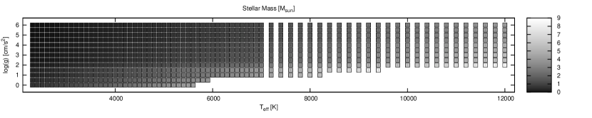
Figure 1: Distribution of stellar masses for that part of the grid with solar abundances for different effective temperatures $T_{\mathrm{eff}}$ and surface gavities $\log(g)$. Color-coded is the stellar mass in units of solar mass from $0M_{\odot}$ (black) to $9M_{\odot}$ (white).

In order to define a spherical symmetric atmosphere as it is used in PHOENIX, we need to define an effective temperature $T_{\mathrm{eff}}$, a surface gravity $\log(g)$ and either a radius $r_{0}$ or a mass $M_{\star}$. We decided to use the mass by taking a mass-luminosity relation $L_{\star}/L_{\odot}=(M_{\star}/M_{\odot})^{3}$ for main-sequence stars and letting it tend towards higher values for giants and super giants:

$$M_{\star}=c\cdot M_{\mathrm{sun}}\cdot\left(\frac{T_{\mathrm{eff}}}{5\,770\,\mathrm{K}}\right)^{2},$$ (1)

with values for the coefficient as given in the following table:

log(g)	$>4$	$>3$	$>2$	$>1.6$	$>0.9$	$>0$	$\leq 0$
c	1	1.2	1.4	2	3	4	5

Figure 1 shows the distribution of masses in our grid for solar abundances.

PHOENIX uses the mixing length theory (Prandtl, 1925; Vitense, 1953) for describing convection within the atmosphere. For our spectra, we used the formula provided by Ludwig et al. (1999), which has been calibrated using 3D RHD models:

$$\alpha=a_{0}+(a_{1}+(a_{3}+a_{5}T_{s}+a_{6}g_{s})T_{s}+a_{4}g_{s})T_{s}+a_{2}g_{s},$$ (2)

with

$$T_{s}=\frac{T_{\mathrm{eff}}-5\,770\,\mathrm{K}}{1\,000}\quad\mathrm{and}\quad g_{s}=\log\left(\frac{10^{\log(g)}}{27\,500}\right),$$ (3)

and coefficients given by:

$a_{0}$	$a_{1}$	$a_{2}$	$a_{3}$	$a_{4}$	$a_{5}$	$a_{6}$
1.587	-0.054	0.045	-0.039	0.176	-0.067	0.107

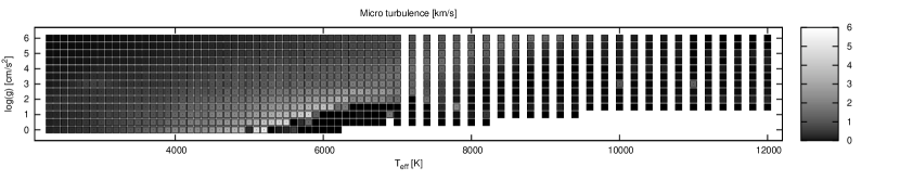
Figure 2: Distribution of micro-turbulences for that part of the grid with solar abundances for different effective temperatures $T_{\mathrm{eff}}$ and surface gavities $\log(g)$. Color-coded is the micro-turbulence from $0\textrm{km/s}$ (black) to $6\textrm{km/s}$ (white).

For matching synthetic spectra with observed ones, we need micro-turbulence as an additional adhoc parameter. Our definition of this is that a large scale (macro-) turbulent motion triggers a small scale (micro-) turbulent motion on length scales below the photon main free path length, which affects the strength of spectral lines (Gray, 2005). In this picture, the micro-turbulence is strongly related to macro-turbulent motion, therefore we use $v_{\mathrm{m}icro}=0.5\cdot\left<v_{\mathrm{c}onv}\right>$ as an experimental formula that follows from 3D radiative hydrodynamic investigations of cool M-stars (Wende et al., 2009). So we first calculate the model atmosphere and then synthesize a spectrum from it using a micro-turbulence, which is assumed to be half the mean convective velocity in the photosphere. Fig. 2 shows the distribution of micro-turbulences in our grid for solar abundances. Unfortunately we had a problem with PHOENIX concerning convection for giants around 7 000 K, so we had to disable convection for those models. Therefore there is no micro-turbulence included as well.

4 Fitting stellar parameters

The spectroscopic analysis of crowded stellar fields, such as star clusters or nearby galaxies has been limited to relatively small samples of stars thus far. The main problem in this respect is that traditionally used techniques like multi-object spectroscopy are restricted to the brighter, isolated stars in the field. We have developed a new method to overcome this limitation using integral field spectroscopy. Taking advantage of the combined spatial and spectral coverage provided by an integral field spectrograph, we developed a new analysis approach which we call “crowded field spectroscopy” (Becker et al., 2004; Kamann, in prep.). Via PSF fitting techniques, single object spectra for the stars above the confusion limit are extracted. This deblending technique works so well that we obtain clean stellar spectra for a significantly higher number of stars than hitherto possible.

For the extracted spectra we determine the stellar parameters using a weighted constrained non-linear least-squares minimization (Levenberg-Marquardt), similar to the ULySS package by Koleva et al. (2009), which has been used as well e. g. by Wu et al. (2011). Usually six different parameters are fitted: effective temperature $T_{\mathrm{eff}}$, surface gravity $\log(g)$, metallicity $[Fe/H]$, $\alpha$-element abundance $[\alpha/Fe]$, radial velocity $v_{\mathrm{rad}}$ and line broadening $\sigma$.

In every iteration of the Levenberg-Marquardt algorithm, a model spectrum is extracted from the PHOENIX grid using an N-dimensional spline interpolator. Then a line of sight velocity distribution (LOSVD) is applied to the model, which adds line broadening $\sigma$ and a shift caused by e. g. radial velocity $v_{\mathrm{rad}}$. Finally an N-dimensional Legendre polynomial (i. e. the continuum difference between model and observation) is determined using a linear fit in a way that the model multiplied with this polynomial matches the observation as best as possible. Due to this we are independent of the continuum and the fit is done on spectral lines only.

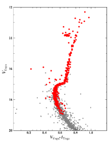
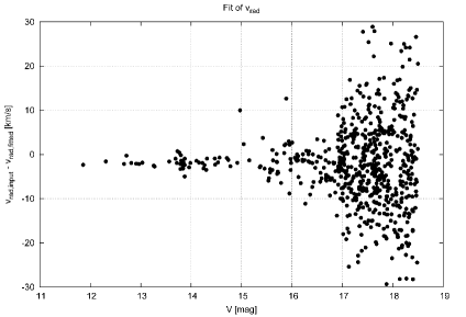
Figure 3: The color-magnitude diagram for a simulated MUSE data cube is shown on the left. For the analysis we only used 1/9 of the cube, for which the stars are marked in red. On the right the errors in fitted radial velocities are plotted.

Figure 3 shows some first preliminary results for a simulated MUSE data cube based on real HST observations of 47 Tuc, obtained by Sarajedini et al. (2007). As one can see, at the main-sequence turnoff point at $\sim$17mag we still can fit the radial velocity with an accuracy of about 5km/s. The systematic offset in the results is caused by a known error in the creation of the simulated data cube. At that magnitude, the corresponding error in the fitted effective temperature is of the order of 100 K.

Kirby et al. (2008) showed that even with medium resolution spectra it is possible to determine the abundance of single elements, in their case it was some of the alpha elements (Mg, Si, Ca, Ti). For this analysis, they created a mask in order to fit only those parts of a spectrum against a grid of synthetic spectra, where it changes most when varying the analysed element. They created the mask by looking for regions, where two spectra with a given $T_{\mathrm{eff}}$, a fixed $\log(g)$, a metallicity of $[Fe/H]=-1.5$ and element abundances of $[X/Fe]=\pm 0.3$ differ by more then $0.5\%$. Masks for several different temperatures where combined into a single mask that was used for the analysis. The main advantage of this method was that they did not need new dimensions in the grid for every new element, but could use an existing one (here $[\alpha/Fe]$), since the masks did not overlap.

With our new PHOENIX grid, we can go one step further and create a mask specifically for every single spectrum that we want to analyse. Therefore we use the same method as described by Kirby et al. (2008), but use the previously fitted values for $T_{\mathrm{eff}}$ and $\log(g)$ of the observed spectrum. Using the individual mask for each star, alpha element abundances can then be determined with an uncertainty of typically 0.1-0.2dex. Of course our intention is to extent this method even further in order to fit the abundance of other elements.

When observing the same field multiple times, we will have radial velocities for several epochs, so that we can determine orbital parameters for binaries that we find. Furthermore we can extend our method described above to fit simultaneously the two components of a binary star and henceforth derive the atmospheric parameters of both stars.

5 Conclusion

We presented a new extensive grid of synthetic stellar spectra from PHOENIX atmospheres with a wavelength range and resolution that should cover all existing and upcoming instruments. Currently its parameter range is optimized for the analysis of globular clusters, but we intend to extend it to higher temperatures. We also introduced a new self-consistent way of describing the micro-turbulence in model atmospheres.

Furthermore we presented a first view on the methods for analyzing globular clusters with data obtained with the VLT MUSE together with preliminary results on simulated data. We showed that we will be able to examine both the kinematics as well as the binary fraction. In addition we will have accurate stellar parameters for most of the stars in the field.

References

- Asplund et al. (2009) Asplund M., Grevesse N., Sauval A. J., Scott P., 2009, ARA&A, 47, 481
- Bacon et al. (2010) Bacon R., et al., 2010, SPIE, 7735,
- Becker et al. (2004) Becker T., Fabrika S., Roth M. M., 2004, AN, 325, 155
- Bedin et al. (2004) Bedin L. R., Piotto G., Anderson J., Cassisi S., King I. R., Momany Y., Carraro G., 2004, ApJ, 605, L125
- Gray (2005) Gray D. F., 2005, The observation and analysis of stellar photospheres (Cambridge University Press)
- Hauschildt & Baron (1999) Hauschildt P. H., Baron E., 1999, JCoAM, 109, 41
- Husser et al. (in prep.) Husser T.-O. et al., 2012, in preparation
- Ivanova et al. (2005) Ivanova N., Belczynski K., Fregeau J. M., Rasio F. A., 2005, MNRAS, 358, 572
- Kaeufl et al. (2004) Kaeufl H.-U., et al., 2004, SPIE, 5492, 1218
- Kamann (in prep.) Kamann S., 2012, in preparation
- Kirby et al. (2008) Kirby E. N., Guhathakurta P., Sneden C., 2008, ApJ, 682, 1217
- Koleva et al. (2009) Koleva M., Prugniel P., Bouchard A., Wu Y., 2009, A&A, 501, 1269
- Lee et al. (1999) Lee Y.-W., Joo J.-M., Sohn Y.-J., Rey S.-C., Lee H.-C., Walker A. R., 1999, Natur, 402, 55
- Ludwig et al. (1999) Ludwig H.-G., Freytag B., Steffen M., 1999, A&A, 346, 111
- Mihalas (1978) Mihalas D., 1978, Stellar atmospheres /2nd edition/, ed. Mihalas, D.
- Portegies Zwart & McMillan (2002) Portegies Zwart S. F., McMillan S. L. W., 2002, ApJ, 576, 899
- Prandtl (1925) Prandtl L., 1925, Zeitschr. Angewandt. Math. Mech., 5, 136
- Sarajedini et al. (2007) Sarajedini A., et al., 2007, AJ, 133, 1658
- Spitzer L. (1987) Spitzer L., Dynamical evolution of globular clusters, ed. Spitzer, L.
- Vernet et al. (2011) Vernet J., et al., 2011, A&A, 536, A105
- Vitense (1953) Vitense E., 1953, ZA, 32, 135
- Wende et al. (2009) Wende S., Reiners A., Ludwig H.-G., 2009, A&A, 508, 1429
- Wu et al. (2011) Wu Y., et al., 2011, RAA, 11, 924