Matrix Representation of Iterative Approximate Byzantine Consensus in Directed Graphs

Abstract

This paper presents a proof of correctness of an iterative approximate Byzantine consensus (IABC) algorithm for directed graphs. The iterative algorithm allows fault-free nodes to reach approximate conensus despite the presence of up to $f$ Byzantine faults. Necessary conditions on the underlying network graph for the existence of a correct IABC algorithm were shown in our recent work [15, 16]. [15] also analyzed a specific IABC algorithm and showed that it performs correctly in any network graph that satisfies the necessary condition, proving that the necessary condition is also sufficient. In this paper, we present an alternate proof of correctness of the IABC algorithm, using a familiar technique based on transition matrices [9, 3, 17, 19].

The key contribution of this paper is to exploit the following observation: for a given evolution of the state vector corresponding to the state of the fault-free nodes, many alternate state transition matrices may be chosen to model that evolution correctly. For a given state evolution, we identify one approach to suitably “design” the transition matrices so that the standard tools for proving convergence can be applied to the Byzantine fault-tolerant algorithm as well. In particular, the transition matrix for each iteration is designed such that each row of the matrix contains a large enough number of elements that are bounded away from 0.

March 8, 2012

1 Introduction

Dolev et al. [5] introduced the notion of approximate Byzantine consensus by relaxing the requirement of exact consensus [14]. The goal in approximate consensus is to allow the fault-free nodes to agree on values that are approximately equal to each other (and not necessarily exactly identical). In presence of Byzantine faults, while exact consensus is impossible in asynchronous systems [7], approximate consensus is achievable [5]. The notion of approximate consensus is of interest in synchronous systems as well, since approximate consensus can be achieved using simple distributed algorithms that do not require complete knowledge of the network topology [4].

In this paper, we are interested in iterative algorithms for achieving approximate Byzantine consensus in synchronous point-to-point networks that are modeled by arbitrary directed  graphs. The iterative approximate Byzantine consensus (IABC) algorithms of interest have the following properties, which we will soon state more formally:

• Initial state of each node is equal to a real-valued input provided to that node.

• Validity condition: After each iteration of an IABC algorithm, the state of each fault-free node must remain in the convex hull of the states of the fault-free nodes at the end of the previous iteration.

• Convergence condition: For any $\epsilon>0$, after a sufficiently large number of iterations, the states of the fault-free nodes are guaranteed to be within $\epsilon$ of each other.

Certain IABC algorithms have been shown to satisfy the above properties in fully connected graphs [5, 14], and in arbitrary directed graphs satisfying a tight necessary condition [15, 16]. Please refer to [15, 16] for a summary of the related work.

The main contribution of this paper is to develop an alternate proof of correctness for a IABC algorithm, which was proved correct in arbitrary graphs that satisfy a necessary condition developed in our prior work [15]. The alternate proof is based on transition matrices that capture the behavior of the IABC algorithm executed by the fault-free nodes. This work is inspired by, and borrows some matrix analysis tools from, other work that also uses transition matrices in related contexts [9, 3, 17, 19]. This paper exploits the following observation: for a given evolution of the state vector corresponding to the state of the fault-free nodes, many alternate state transition matrices may potentially be chosen to emulate that evolution correctly. For a given state evolution, we identify one approach to suitably “design” the transition matrices so that the standard tools can be applied to prove convergence of the Byzantine fault-tolerant algorithm in all networks that satisfy a necessary condition (proved in [16]) on the network communication graph. In particular, the transition matrix for each iteration is designed such that each row of the matrix contains a large enough number of elements that are bounded away from 0.

2 Network and Failure Models

Network Model:

The system is assumed to be synchronous. The communication network is modeled as a simple directed graph $G(\mathcal{V},\mathcal{E})$, where $\mathcal{V}=\{1,\dots,n\}$ is the set of $n$ nodes, and $\mathcal{E}$ is the set of directed edges between the nodes in $\mathcal{V}$. Node $i$ can reliably transmit messages to node $j$ if and only if the directed edge $(i,j)$ is in $\mathcal{E}$. Each node can send messages to itself as well, however, for convenience, we exclude self-loops from set $\mathcal{E}$. That is, $(i,i)\not\in\mathcal{E}$ for $i\in\mathcal{V}$. With a slight abuse of terminology, we will use the terms edge and link interchangeably in our presentation.

For each node $i$, let $N_{i}^{-}$ be the set of nodes from which $i$ has incoming edges. That is, $N_{i}^{-}=\{\,j~{}|~{}(j,i)\in\mathcal{E}\,\}$. Similarly, define $N_{i}^{+}$ as the set of nodes to which node $i$ has outgoing edges. That is, $N_{i}^{+}=\{\,j~{}|~{}(i,j)\in\mathcal{E}\,\}$. Since we exclude self-loops from $\mathcal{E}$, $i\not\in N_{i}^{-}$ and $i\not\in N_{i}^{+}$. However, we note again that each node can indeed send messages to itself. A necessary condition for correctness of an IABC algorithm for $f>0$ is that $|N_{i}^{-}|>2f$ [15].

Node $j$ is said to be an incoming neighbor of node $i$, if $j\in N_{i}^{-}$. Similarly, $j$ is said to be an outgoing neighbor of node $i$, if $j\in N_{i}^{+}$.

Failure Model:

We consider the Byzantine failure model, with up to $f$ nodes becoming faulty. A faulty node may misbehave arbitrarily. Possible misbehavior includes sending incorrect and mismatching (or inconsistent) messages to different neighbors. The faulty nodes may potentially collaborate with each other. Moreover, the faulty nodes are assumed to have a complete knowledge of the execution of the algorithm, including the states of all the nodes, contents of messages the other nodes send to each other, the algorithm specification, and the network topology.

3 Iterative Approximate Byzantine Consensus (IABC)

Each node $i$ maintains state $v_{i}$, with $v_{i}[t]$ denoting the state of node $i$ at the end  of the $t$-th iteration of the algorithm. Initial state of node $i$, $v_{i}[0]$, is equal to the initial input  provided to node $i$. At the start of the $t$-th iteration ($t>0$), the state of node $i$ is $v_{i}[t-1]$.

Let $\mathcal{F}$ denote the set of faulty nodes. Thus, the nodes in $\mathcal{V}-\mathcal{F}$ are non-faulty.

• $U[t]=\max_{i\in\mathcal{V}-\mathcal{F}}\,v_{i}[t]$. $U[t]$ is the largest state among the fault-free nodes at the end of the $t$-th iteration. Since the initial state of each node is equal to its input, $U[0]$ is equal to the maximum value of the initial input at the fault-free nodes.

• $\mu[t]=\min_{i\in\mathcal{V}-\mathcal{F}}\,v_{i}[t]$. $\mu[t]$ is the smallest state among the fault-free nodes at the end of the $t$-th iteration. $\mu[0]$ is equal to the minimum value of the initial input at the fault-free nodes.

The following conditions must be satisfied by an IABC algorithm in presence of up to $f$ Byzantine faulty nodes:

• Validity: $\forall t>0,~{}~{}\mu[t]\geq\mu[t-1]~{}\mbox{~{}~{}and~{}~{}}~{}~{}U[t]\leq U[t-1]$

• Convergence: $\lim_{\,t\rightarrow\infty}~{}U[t]-\mu[t]=0$. Equivalently, $\lim_{\,t\rightarrow\infty}~{}v_{i}[t]-v_{j}[t]=0$, for $i,j\in\mathcal{V}-\mathcal{F}$.

An iterative algorithm is said to be correct if it satisfies the validity and convergence conditions. We will prove the correctness of Algorithm 1 below in all graphs that satisfy the necessary condition in Theorem 2 of [16]. The algorithm should be performed by each node $i$ in the $t$-th iteration, $t\geq 1$. The faulty nodes may deviate from the algorithm specification. If a fault-free node does not receive an expected message from an incoming neighbor (in the Receive step below), then that message is assumed to have some default value.

 

Algorithm 1  

Steps to be performed by node $i$ in the $t$-th iteration:

1. Transmit step: Transmit current state $v_{i}[t-1]$ on all outgoing edges.

2. Receive step: Receive values on all incoming edges. These values form vector $r_{i}[t]$ of size $|N_{i}^{-}|$.

3. Update step: Sort the values in $r_{i}[t]$ in an increasing order, and eliminate the smallest $f$ values, and the largest $f$ values (breaking ties arbitrarily). Let $N_{i}^{*}[t]$ denote the identifiers of nodes from whom the remaining $|N_{i}^{-}|-2f$ values were received, and let $w_{j}$ denote the value received from node $j\in N_{i}^{*}[t]$.

   For convenience, define $w_{i}=v_{i}[t-1]$.

   Observe that if $j\in\{i\}\cup N_{i}^{*}[t]$ is fault-free, then $w_{j}=v_{j}[t-1]$.

   Define

   $$v_{i}[t]~{}=~{}\sum_{j\in\{i\}\cup N_{i}^{*}[t]}a_{i}\,w_{j}$$ (1)

   where

   $$a_{i}~{}=~{}\frac{1}{|N_{i}^{-}|-2f+1}~{}=~{}\frac{1}{|N_{i}^{*}[t]|+1}$$

   Recall that $i\not\in N_{i}^{*}[t]$ because $(i,i)\not\in\mathcal{E}$. The “weight” of each term on the right-hand side of (1) is $a_{i}$, and these weights add to 1.

   Observe that $0<a_{i}\leq 1$.

   For future reference, let us define $\alpha$ as:

   $$\alpha=\min_{i\in\mathcal{V}}~{}a_{i}$$ (2)

   Note that $0<\alpha\leq 1$. Specifically, $\alpha$ is a positive constant that is dependent only on $f$ and the graph $G(\mathcal{V},\mathcal{E})$.

 

Similar algorithms have been proven to work correctly in fully connected graphs [5, 15] and arbitrary directed graphs satisfying the necessary condition stated in [15]. In this paper, we provide an alternate proof of correctness in such arbitrary graphs, using an alternate form of the necessary condition [16].

4 Matrix Preliminaries

We use boldface upper case letters to denote matrices, rows of matrices, and their elements. For instance, ${\bf H}$ denotes a matrix, ${\bf H}_{i}$ denotes the $i$-th row of matrix ${\bf H}$, and ${\bf H}_{ij}$ denotes the element at the intersection of the $i$-th row and the $j$-th column of matrix ${\bf H}$.

Definition 1

A vector is said to be stochastic if all the elements of the vector are non-negative, and the elements add up to 1. A matrix is said to be row stochastic if each row of the matrix is a stochastic vector.

For a row stochastic matrix ${\bf A}$, coefficients of ergodicity $\delta({\bf A})$ and $\lambda({\bf A})$ are defined as [18]:

$$\delta({\bf A}) :=\max_{j}~{}\max_{i_{1},i_{2}}~{}|{\bf A}_{i_{1}\,j}-{\bf A}_{i_{2}\,j}|,$$ (3)

$$\lambda({\bf A}) :=1-\min_{i_{1},i_{2}}\sum_{j}\min({\bf A}_{i_{1}\,j}~{},{\bf A}_{i_{2}\,j}).$$ (4)

It is easy to see that $0\leq\delta({\bf A})\leq 1$ and $0\leq\lambda({\bf A})\leq 1$, and that the rows are all identical if and only if $\delta({\bf A})=0$. Additionally, $\lambda({\bf A})=0$ if and only if $\delta({\bf A})=0$.

The next result from [8] establishes a relation between the coefficient of ergodicity $\delta(\cdot)$ of a product of row stochastic matrices, and the coefficients of ergodicity $\lambda(\cdot)$ of the individual matrices defining the product.

Claim 1

For any $p$ square row stochastic matrices ${\bf Q}(1),{\bf Q}(2),\dots\bf Q(p)$,

$$\delta({\bf Q}(1){\bf Q}(2)\cdots{\bf Q}(p))~{}\leq~{}\Pi_{i=1}^{p}~{}\lambda({\bf Q}(i)).$$ (5)

Claim 1 is proved in [8]. It implies that if, for all $i$, $\lambda({\bf Q}(i))\leq 1-\gamma$ for some $\gamma>0$, then $\delta({\bf Q}(1),{\bf Q}(2)\cdots{\bf Q}(p))$ will approach zero as $p$ approaches $\infty$.

Definition 2

A row stochastic matrix ${\bf H}$ is said to be a scrambling  matrix, if $\lambda({\bf H})<1$ [8, 18].

In a scrambling matrix ${\bf H}$, since $\lambda({\bf H})<1$, for each pair of rows $i_{1}$ and $i_{2}$, there exists a column $j$ (which may depend on $i_{1}$ and $i_{2}$) such that ${\bf H}_{i_{1}\,j}>0$ and ${\bf H}_{i_{2}\,j}>0$, and vice-versa [8, 18]. As a special case, if any one column of a row stochastic matrix ${\bf H}$ contains only non-zero elements that are lower bounded by some constant $\gamma>0$, then ${\bf H}$ must be scrambling, and $\lambda({\bf H})\leq 1-\gamma$.

5 Matrix Representation of Algorithm 1

Recall that $\mathcal{F}$ is the set of faulty nodes. Let $|\mathcal{F}|=\phi$. Without loss of generality, suppose that nodes 1 through $(n-\phi)$ are fault-free, and if $\phi>0$, nodes $(n-\phi+1)$ through $n$ are faulty.

Denote by ${\bf v}[0]$ the column vector consisting of the initial states of all the fault-free nodes. Denote by ${\bf v}[t]$, where $t\geq 1$, the column vector consistsing of the states of all the fault-free nodes at the end of the $t$-th iteration, $t\geq 1$. The $i$-th element of vector ${\bf v}[t]$ is state $v_{i}[t]$. The size of the column vector ${\bf v}[t]$ is $(n-\phi)$.

Claim 2

We can express the iterative update of the state of a fault-free node $i$ $(1\leq i\leq n-\phi)$ performed in (1) using the matrix form in (6) below, where ${\bf M}_{i}[t]$ satisfies the following four conditions.

$$v_{i}[t] = {\bf M}_{i}[t]~{}{{\bf v}}[t-1]$$ (6)

In addition to $t$, the row vector ${\bf M}_{i}[t]$ may depend on the state vector ${\bf v}[t-1]$ as well as the behavior of the faulty nodes in $\mathcal{F}$. For simplicity, the notation ${\bf M}_{i}[t]$ does not explicitly represent this dependence.

1. ${\bf M}_{i}[t]$ is a stochastic row vector of size $(n-\phi)$. Thus, ${\bf M}_{ij}[t]\geq 0$, for $1\leq j\leq n-\phi$, and

   $$\sum_{1\leq j\leq n-\phi}~{}{\bf M}_{ij}[t]~{}=~{}1$$

2. ${\bf M}_{ii}[t]$ equals $a_{i}$ defined in Algorithm 1. Recall that $a_{i}\geq\alpha$.

3. ${\bf M}_{ij}[t]$ is non-zero only if $(j,i)\in\mathcal{E}$ or $j=i$.

4. At least $|N_{i}^{-}\cap\,(\mathcal{V}-\mathcal{F})|-f+1$ elements in ${\bf M}_{i}[t]$ are lower bounded by some constant $\beta>0$, to be defined later ($\beta$ is independent of $i$). Note that $N_{i}^{-}\cap\,(\mathcal{V}-\mathcal{F})$ is the set of fault-free incoming neighbors of node $i$.

Proof:

The proof of this claim is presented in Section 5.1 below. The last condition above plays an important role in the proof, and the main contribution of this paper is to “design” ${\bf M}_{i}[t]$ to make this condition true. $\Box$

By “stacking” (6) for different $i$, $1\leq i\leq n-\phi$, we can represent the state update for all the fault-free nodes together using (7) below, where ${\bf M}[t]$ is a $(n-\phi)\times(n-\phi)$ matrix, with its $i$-th row being equal to ${\bf M}_{i}[t]$ in (6).

$${{\bf v}}[t] = {\bf M}[t]~{}{{\bf v}}[t-1]$$ (7)

The four properties of ${\bf M}_{i}[t]$ imply that ${\bf M}[t]$ is a row stochastic matrix with a non-zero diagonal. Also, the $i$-th row of ${\bf M}[t]$ contains $|N_{i}^{-}\cap\,(\mathcal{V}-\mathcal{F})|-f+1$ elements lower bounded by $\beta$ ($\beta$ will be defined later). This property of ${\bf M}[t]$ turns out to be important in proving convergence of Algorithm 1.

${\bf M}[t]$ is said to be a transition matrix.

By repeated application of (7), we obtain:

$${\bf v}[t] = \left(\,\Pi_{i=1}^{t}{\bf M}[i]\,\right)\,{\bf v}[0]$$

5.1 Correctness of Claim 2

Figure 1 illustrates the various sets used here. Some of the sets in this figure are not yet defined, and will be defined later in the paper.

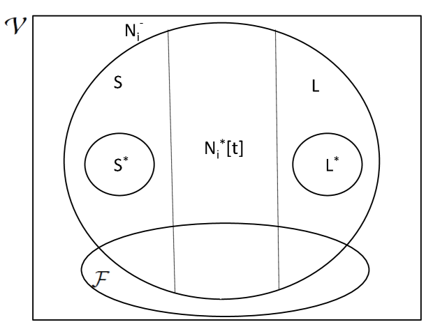
Figure 1: Illustration of sets $\mathcal{V}$, $\mathcal{F}$, $N_{i}^{-}$, $N_{i}^{*}[t]$, $L^{*}$ and $S^{*}$

We prove the correctness of Claim 2 by constructing ${\bf M}_{i}[t]$ for $1\leq i\leq n-\phi$ that satisfies the conditions in Claim 2. Recall that nodes 1 through $n-\phi$ are fault-free, and the remaining $\phi$ nodes ($\phi\leq f$) are faulty.

Consider a fault-free node $i$ performing the Update step in Algorithm 1. Recall that the largest $f$ and the smallest $f$ values are eliminated from $r_{i}[t]$. Let us denote by $L$ and $S$, respectively, the set of nodes from whom the largest $f$ values and the smallest $f$ values were received by node $i$ in iteration $t$. Thus, $|L|=|S|=f$, $N_{i}^{*}[t]=N_{i}^{-}-(L\cup S)$, and $|N_{i}^{*}[t]|=|N_{i}^{-}-(L\cup S)|=|N_{i}^{-}|-2f$.

For any set of nodes $X$ here, let $\delta_{X}$ and $g_{X}$ respectively denote the number of faulty nodes, and the number of fault-free nodes, in set $X$. For instance, $\delta_{L}$ and $g_{L}$ denote, respectively, the number of faulty and fault-free nodes in set $L$. Thus,

$$\delta_{L}+g_{L}~{}=~{}\delta_{S}+g_{S}~{}=~{}f$$

Let

$$\delta=|N_{i}^{-}\cap\mathcal{F}|$$

That is, the number of faulty incoming neighbors of node $i$ is denoted as $\delta$. Therefore, $\delta\leq\phi\leq f$, and

$$\delta=\delta_{L}+\delta_{S}+\delta_{N_{i}^{*}[t]}$$

Then, it follows that

$$g_{L} = f-\delta_{L}~{}=~{}\delta_{S}+\delta_{N_{i}^{*}[t]}+(f-\delta),\mbox{~{}and}$$ (8)

$$g_{S} = f-\delta_{S}~{}=~{}\delta_{L}+\delta_{N_{i}^{*}[t]}+(f-\delta)$$ (9)

For fault-free node $i$, we now define the elements of row ${\bf M}_{i}[t]$. We consider two cases separately: (i) $f-\delta+\delta_{N_{i}^{*}[t]}=0$, and (ii) $f-\delta+\delta_{N_{i}^{*}[t]}>0$.

5.1.1 $f-\delta+\delta_{N_{i}^{*}[t]}=0$

We know that $(f-\delta)\geq 0$ and $\delta_{N_{i}^{*}[t]}\geq 0$. Therefore, $f-\delta+\delta_{N_{i}^{*}[t]}=0$ implies that $f=\delta$ and $\delta_{N_{i}^{*}[t]}=0$. Thus, in this case, all the nodes in $N_{i}^{*}[t]$ are fault-free.

• For each $j\in\{i\}\cup N_{i}^{*}[t]$, define ${\bf M}_{ij}[t]=a_{i}$. Element ${\bf M}_{ij}[t]$ corresponds to the term $a_{i}w_{j}$ in (1).

  Recall that $a_{i}\geq\alpha$, and that each node in $\{i\}\cup N_{i}^{*}[t]$ in this case is fault-free.

• For each $j$ such that $j\in\mathcal{V}-\mathcal{F}$ and $j\not\in\{i\}\cup N_{i}^{*}[t]$, define ${\bf M}_{ij}[t]=0$.

Observe that with the above definition of elements of ${\bf M}_{i}[t]$,

$${\bf M}_{i}[t]{\bf v}[t-1]=\sum_{k\in\{i\}\cup N_{i}^{*}[t]}a_{i}w_{k}$$

In the above procedure, we have set $|N_{i}^{*}[t]|+1$ elements of ${\bf M}_{i}[t]$ equal to $a_{i}$ (recall that $a_{i}\geq\alpha$).

Now, because $\delta=f$ and $|N_{i}^{*}[t]|=|N_{i}^{-}|-2f$, we have $|N_{i}^{-}\cap(\mathcal{V}-\mathcal{F})|-f+1=|N_{i}^{-}|-\delta-f+1=|N_{i}^{-}|-2f+1=|N_{i}^{*}[t]|+1$. Also, in this case $a_{i}=1/(|N_{i}^{*}[t]|+1)$. Thus, it should be easy to see that the conditions in Claim 2 are satisfied by defining $\beta=\alpha$.

5.1.2 $f-\delta+\delta_{N_{i}^{*}[t]}>0$

Since $0\leq\delta_{N_{i}^{*}[t]}\leq\delta\leq f$, $f-\delta+\delta_{N_{i}^{*}[t]}>0$ implies that $f>0$. When $f>0$, the necessary condition in [15] implies that $|N_{i}^{-}|\geq 2f+1$. Therefore, the set $N_{i}^{*}[t]$ is non-empty. As per (1), each node $k\in N_{i}^{*}[t]$ contributes $a_{i}\,w_{k}$ to the new state $v_{i}[t]$ of node $i$. We will define elements of ${\bf M}_{i}[t]$ to account for the contribution of each node $k\in N_{i}^{*}[t]$.

Define subsets $L^{*}$ and $S^{*}$ such that $L^{*}\subseteq L$, $S^{*}\subseteq S$, $L^{*}\cap\mathcal{F}=S^{*}\cap\mathcal{F}=\Phi$, and $|L^{*}|=|S^{*}|=f-\delta+\delta_{N_{i}^{*}[t]}$. That is, sets $L^{*}$ and $S^{*}$ are subsets of $L$ and $S$, respectively, each of size $f-\delta+\delta_{N_{i}^{*}[t]}$, and containing only fault-free nodes. Expressions (8) and (9) for $g_{L}$ and $g_{S}$ imply that such subsets exist.

Let

$$L^{*}=\{l_{j}~{}|~{}1\leq j\leq f-\delta+\delta_{N_{i}^{*}[t]}\}$$

and

$$S^{*}=\{s_{j}~{}|~{}1\leq j\leq f-\delta+\delta_{N_{i}^{*}[t]}\}.$$

Consider any node $k\in N_{i}^{*}[t]$. For each $j$, $1\leq j\leq f-\delta+\delta_{N_{i}^{*}[t]}$,

$$v_{s_{j}}[t-1]\leq w_{k}\leq v_{l_{j}}[t-1]$$

Therefore, we can find weights $\lambda_{k,j}\geq 0$ and $\psi_{k,j}\geq 0$ such that

$$\lambda_{k,j}+\psi_{k,j}~{}=~{}1$$

and

$$w_{k}~{}=~{}~{}\lambda_{k,j}\,v_{l_{j}}[t-1]~{}+~{}\psi_{k,j}\,v_{s_{j}}[t-1]$$

Clearly, at least one of the weights $\lambda_{k,j}$ and $\psi_{k,j}$ must be $\geq 1/2$. Now, observe that

$$a_{i}\,w_{k} = \frac{a_{i}}{f-\delta+\delta_{N_{i}^{*}[t]}}~{}\sum_{1\leq j\leq f-\delta+\delta_{N_{i}^{*}[t]}}\left(\lambda_{k,j}\,v_{l_{j}}[t-1]+\psi_{k,j}\,v_{s_{j}}[t-1]\right)$$ (10)

The above equality is true independent of whether $k$ is fault-free or faulty. We will later use the above equality for the case when $k$ is a faulty node. When $k$ is fault-free,

$$w_{k}=v_{k}[t-1],$$

and we can similarly obtain the equality below.

$$a_{i}w_{k} = \frac{a_{i}}{2}v_{k}[t-1]~{}+~{}\frac{a_{i}}{2(f-\delta+\delta_{N_{i}^{*}[t]})}~{}\sum_{1\leq j\leq f-\delta+\delta_{N_{i}^{*}[t]}}\left(\lambda_{k,j}\,v_{l_{j}}[t-1]+\psi_{k,j}\,v_{s_{j}}[t-1]\right)$$

We now use (1), (10) and (LABEL:e_faultfree) to define elements of ${\bf M}_{i}[t]$ in the following four cases:

• Case 1: Node $i$
  Define ${\bf M}_{ii}[t]=a_{i}$. This is obtained by observing in (1) that the contribution of node $i$ to the new state $v_{i}[t]$ is $a_{i}w_{i}=a_{i}v_{i}[t-1]$.

• Case 2: Fault-free nodes in $N_{i}^{*}[t]$
  For each $k\in N_{i}^{*}[t]\cap(\mathcal{V}-\mathcal{F})$, define ${\bf M}_{ik}[t]=\frac{a_{i}}{2}$. This choice is motivated by (LABEL:e_faultfree) wherein the contribution of node $k$ to $a_{i}w_{k}$ is $\frac{a_{i}}{2}v_{k}[t-1]$. In Case 2, $|N_{i}^{*}[t]\cap(\mathcal{V}-\mathcal{F})|=|N_{i}^{-}|-\delta$ elements of ${\bf M}_{i}[t]$ are defined.

• Case 3: Nodes in $L^{*}$ and $S^{*}$
  For $1\leq j\leq f-\delta+\delta_{N_{i}^{*}[t]}$, consider $l_{j}\in L^{*}$. In this case,

  $${\bf M}_{il_{j}}[t] = \sum_{k\in N_{i}^{*}[t]\cap\mathcal{F}}\frac{a_{i}}{f-\delta+\delta_{N_{i}^{*}[t]}}\lambda_{k,j}~{}+~{}\sum_{k\in N_{i}^{*}[t]\cap(\mathcal{V}-\mathcal{F})}\frac{a_{i}}{2(f-\delta+\delta_{N_{i}^{*}[t]})}\lambda_{k,j}$$

  Similarly, for $1\leq j\leq f-\delta+\delta_{N_{i}^{*}[t]}$, consider $s_{j}\in S^{*}$. In this case,

  $${\bf M}_{is_{j}}[t] = \sum_{k\in N_{i}^{*}[t]\cap\mathcal{F}}\frac{a_{i}}{f-\delta+\delta_{N_{i}^{*}[t]}}\psi_{k,j}~{}+~{}\sum_{k\in N_{i}^{*}[t]\cap(\mathcal{V}-\mathcal{F})}\frac{a_{i}}{2(f-\delta+\delta_{N_{i}^{*}[t]})}\psi_{k,j}$$

  These expressions are obtained by summing (10) and (LABEL:e_faultfree), respectively, over the faulty and fault-free nodes in $N_{i}^{*}[t]$, and then identifying the contribution of each node in $L^{*}$ and $S^{*}$ to this sum. Recall the earlier observation that at least one of $\lambda_{k,j}$ and $\psi_{k,j}$ must be $\geq 1/2$ for each pair $k,j$ where $k\in N_{i}^{*}[t]$ and $1\leq j\leq f-\delta+\delta_{N_{i}^{*}[t]}$. Therefore, it follows that at least $f-\delta+\delta_{N_{i}^{*}[t]}$ elements of ${\bf M}_{i}[t]$ defined in Case 3 must be $\geq\frac{a_{i}}{4(f-\delta+\delta_{N_{i}^{*}[t]})}$.

• Case 4: Nodes in $(\mathcal{V}-\mathcal{F})-(\{i\}\cup N_{i}^{*}[t]\cup L^{*}\cup S^{*})$
  These fault-free nodes have not yet been considered in Cases 1, 2 and 3. For each node $k\in(\mathcal{V}-\mathcal{F})-(\{i\}\cup N_{i}^{*}[t]\cup L^{*}\cup S^{*})$, we assign ${\bf M}_{ik}[t]=0$.

Observe that above the definition of the elements of ${\bf M}_{i}[t]$ ensures that

$$\sum_{j\in\{i\}\cup N_{i}^{*}[t]}a_{i}w_{j}~{}=~{}{\bf M}_{i}[t]{\bf v}[t-1]$$

However, the contribution by the faulty nodes in $N_{i}^{*}[t]$ in (1) is now replaced by an equivalent contribution by the nodes in $L^{*}$ and $S^{*}$.

Now let us verify that the four conditions in Claim 2 hold for the above assignments to the elements of ${\bf M}_{i}[t]$.

1. Observe that all the elements of ${\bf M}_{i}[t]$ are non-negative. Case 1 specifies just ${\bf M}_{ii}[t]=a_{i}$. The elements of ${\bf M}_{i}[t]$ specified in Case 2 add up to

   $$\frac{a_{i}}{2}~{}|N_{i}^{*}[t]\cap(\mathcal{V}-\mathcal{F})|$$

   Recall that for each $j$, $1\leq j\leq(f-\delta+\delta_{N_{i}^{*}[t]})$, $\lambda_{k,j}+\psi_{k,j}=1$ for $k\in N_{i}^{*}[t]$. Therefore, when added over all $k\in N_{i}^{*}[t]$ and $1\leq j\leq(f-\delta+\delta_{N_{i}^{*}[t]})$, the elements of ${\bf M}_{i}[t]$ specified in Case 3 add up to

   $$a_{i}~{}|N_{i}^{*}[t]\cap\mathcal{F}|~{}+~{}\frac{a_{i}}{2}~{}|N_{i}^{*}[t]\cap(\mathcal{V}-\mathcal{F})|$$

   Therefore, when all the elements of ${\bf M}_{i}[t]$ defined in Cases 1, 2 and 3 are added together, we get

   $$a_{i}~{}+~{}a_{i}\,|N_{i}^{*}[t]\cap\mathcal{F}|~{}+~{}a_{i}|N_{i}^{*}[t]\cap(\mathcal{V}-\mathcal{F})|~{}=~{}a_{i}(|N_{i}^{*}[t]|+1)~{}=~{}1$$

   because $a_{i}=1/(|N_{i}^{*}[t]|+1)$. Now observe that the elements specified in Cases 1, 2 and 3 are clearly $\leq 1$. In the expression for ${\bf M}_{il_{j}}[t]$ in Case 3, observe that the two summations on the right side together contain $|N_{i}^{*}[t]|$ terms, and in these terms, observe that $\lambda_{k,j}\leq 1$, $f-\delta+\delta_{N_{i}^{*}[t]}\geq 1$ and $a_{i}=\frac{1}{|N_{i}^{*}[t]|+1}$. Therefore, ${\bf M}_{il_{j}}[t]<1$. Similarly, we can show that ${\bf M}_{is_{j}}[t]<1$ as well.

   Thus, we have shown that ${\bf M}_{i}[t]$ is a stochastic vector.

2. ${\bf M}_{ii}[t]=a_{i}$ as specified in Case 1.

3. Since ${\bf M}_{ij}[t]$ is defined to be non-zero only in Cases 1, 2 and 3, which consider the nodes only in $\{i\}\cup N_{i}^{-}$, it follows that ${\bf M}_{ij}[t]$ is non-zero only if $(j,i)\in\mathcal{E}$ or $j=i$.

4. Cases 1 and 2 together set $1+|N_{i}^{*}[t]\cap(\mathcal{V}-\mathcal{F})|=1+|N_{i}^{*}[t]|-\delta_{N_{i}^{*}[t]}$ elements of ${\bf M}_{i}[t]$ to be $\geq a_{i}/2$. We observed earlier that Case 3 results in at least $f-\delta+\delta_{N_{i}^{*}[t]}$ elements of ${\bf M}_{i}[t]$ being $\geq\frac{a_{i}}{4(f-\delta+\delta_{N_{i}^{*}[t]})}$. Also, observe that the elements of ${\bf M}_{i}[t]$ specified in Cases 1 and 2 are distinct from those specified in Case 3, and that $\frac{a_{i}}{2}\geq\frac{a_{i}}{4(f-\delta+\delta_{N_{i}^{*}[t]})}$. Thus, overall, at least

   $$(1+|N_{i}^{*}[t]|-\delta_{N_{i}^{*}[t]})~{}+~{}f-\delta+\delta_{N_{i}^{*}[t]}~{}=~{}|N_{i}^{*}[t]|+f-\delta+1~{}=~{}|N_{i}^{-}|-f-\delta+1$$

   $$~{}=~{}|N_{i}^{-}\cap(\mathcal{V}-\mathcal{F})|-f-1$$

   elements of ${\bf M}_{i}[t]$ are set $\geq\frac{a_{i}}{4(f-\delta+\delta_{N_{i}^{*}[t]})}$. Derivation of the above equation uses the facts that $|N_{i}^{*}[t]|=|N_{i}^{-}|-2f$ and $|N_{i}^{-}\cap(\mathcal{V}-\mathcal{F})|=|N_{i}^{-}|-\delta$. Then by defining $\beta$ as below, condition 4 in Claim 2 holds true.

   $$\beta=\frac{\alpha}{4(f-\delta+\delta_{N_{i}^{*}[t]})}$$

Therefore, Claim 2 is proved correct.

5.2 Correspondence Between Sufficiency Condition and $\bf M[t]$

Let us define set $R_{\mathcal{F}}$ of subgraphs of $G(\mathcal{V},\mathcal{E})$ as follows.

$$R_{\mathcal{F}} = \{H~{}|~{}H\mbox{~{} is obtained by removing all the faulty}$$ (12)

nodes from $$\mathcal{V}$$ along with their edges, and then

removing any additional $$f$$ incoming edges

$$\mbox{ at each fault-free node}\}$$

Thus, $\mathcal{V}-\mathcal{F}$ is the set of nodes in each graph in $R_{\mathcal{F}}$.

Let $\tau$ denote $|R_{\mathcal{F}}|$. $\tau$ depends on $\mathcal{F}$ and the underlying network, and it is finite.

Claim 3

Suppose that graph $G(\mathcal{V},\mathcal{E})$ satisfies the necessary condition in Theorem 2 in [16]. Then it follows that in each $H\in R_{\mathcal{F}}$, there exists at least one node that has directed paths to all the nodes in $H$ (consisting of the edges in $H$).

Proof:

The proof follows from Theorem 2 of [16]. $\Box$

In this discussion, let us denote a graph by an italic upper case letter, and the corresponding connectivity matrix using the same letter in boldface upper case. Thus, ${\bf H}$ will denote the connectivity matrix for graph $H\in R_{\mathcal{F}}$; ${\bf H}$ is defined as follows: (i) for $1\leq i,j\leq n-\phi$, if there is a directed link from node $j$ to node $i$ in graph $H$ then ${\bf H}_{ij}=1$, and (ii) ${\bf H}_{ii}=1$ for $1\leq i\leq n-\phi$. Note that in our notation, the $i$-th row of ${\bf H}$ (that is, ${\bf H}_{i}$) corresponds to the incoming links at node $i$, and the self-loop at node $i$. The connectivity matrix ${\bf H}$ for any $H\in R_{\mathcal{F}}$ has a non-zero diagonal.

Lemma 1

For any $H\in R_{\mathcal{F}}$, ${\bf H}^{n-\phi}$ has at least one non-zero column.

Proof:

By Claim 3, in graph $H$ there exists at least one node, say node $k$, that has a directed path in $H$ to all the remaining nodes in $H$. Since the length of the path from $k$ to any other node in $H$ can contain at most $n-\phi-1$ directed edges, the $k$-th column of matrix ${{\bf H}^{n-\phi}}$ will be non-zero. $\Box$

Definition 3

We will say that an element of a matrix is “non-trivial” if it is lower bounded by $\beta$.

Definition 4

For matrices ${\bf A}$ and ${\bf B}$ of identical size, and a scalar $\gamma$, ${\bf A}\leq\gamma\,{\bf B}$ provided that ${\bf A}_{ij}\leq\gamma\,{\bf B}_{ij}$ for all $i,j$.

Lemma 2

For any $t\geq 1$, there exists a graph $H[t]\in R_{\mathcal{F}}$ such that $\beta\,{\bf H}[t]~{}\leq~{}{{\bf M}[t]}$.

Proof:

Observe that the $i$-th row of the transition matrix ${\bf M}[t]$ corresponds to the state update performed at fault-free node $i$. Recall from Claim 2 that the ${\bf M}_{ij}$ is non-zero only if link $(j,i)\in\mathcal{E}$. Also, by Claim 2, ${\bf M}_{i}[t]$ (i.e., the $i$-th row of ${\bf M}[t]$) contains at least $|N_{i}^{-}\cap\,(\mathcal{V}-\mathcal{F})|-f+1$ non-trivial elements corresponding to fault-free incoming neighbors of node $i$ and itself (i.e., the diagonal element).

Now observe that, for any subgraph $H\in R_{\mathcal{F}}$, $i$-th row of ${\bf H}$ contains exactly $|N_{i}^{-}\cap\,(\mathcal{V}-\mathcal{F})|-f+1$ non-zero elements, including the diagonal element.

Considering the above two observations, and the definition of set $R_{\mathcal{F}}$, the lemma follows. $\Box$

6 Correctness of Algorithm 1

The proof below uses techniques also applied in prior work (e.g., [9, 3, 17, 19]), with some similarities to the arguments used in [17, 19].

Lemma 3

In the product below of ${\bf H}[t]$ matrices for consecutive $\tau(n-\phi)$ iterations, at least one column is non-zero.

$$\Pi_{t=z}^{z+\tau(n-\phi)-1}\,{\bf H}[t]$$

Proof:

Since the above product consists of $\tau(n-\phi)$ matrices in $R_{\mathcal{F}}$, at least one of the $\tau$ distinct connectivity matrices in $R_{\mathcal{F}}$, say matrix ${\bf H}_{*}$, will appear in the above product at least $n-\phi$ times.

Now observe that: (i) By Lemma 1, ${\bf H}_{*}^{n-\phi}$ contains a non-zero column, say the $k$-th column is non-zero, and (ii) all the ${\bf H}[t]$ matrices in the product contain a non-zero diagonal. These two observations together imply that the $k$-th column in the above product is non-zero. $\Box$

Let us now define a sequence of matrices ${\bf Q}(i)$ such that each of these matrices is a product of $\tau(n-\phi)$ of the ${\bf M}[t]$ matrices. Specifically,

$${\bf Q}(i)~{}=~{}\Pi_{t=(i-1)\tau(n-\phi)+1}^{i\tau(n-\phi)}~{}{\bf M}[t]$$

Observe that

$${\bf v}[k\tau(n-\phi)] = \left(\,\Pi_{i=1}^{k}~{}{\bf Q}(i)\,\right)~{}{\bf v}[0]$$ (13)

Lemma 4

For $i\geq 1$, ${\bf Q}(i)$ is a scrambling row stochastic matrix, and $\lambda({\bf Q}(i))$ is bounded from above by a constant smaller than 1.

Proof:

${\bf Q}(i)$ is a product of row stochastic matrices (${\bf M}[t]$), therefore, ${\bf Q}(i)$ is row stochastic.

From Lemma 2, for each $t$,

$$\beta\,{\bf H}[t]~{}\leq~{}{\bf M}[t]$$

Therefore,

$$\beta^{\tau(n-\phi)}~{}\Pi_{t=(i-1)\tau(n-\phi)+1}^{i\tau(n-\phi)}~{}{\bf H}[t]~{}\leq~{}{\bf Q}(i)$$

By using $z=(i-1)(n-\phi)+1$ in Lemma 3, we conclude that the matrix product on the left side of the above inequality contains a non-zero column. Therefore, ${\bf Q}(i)$ contains a non-zero column as well. Therefore, ${\bf Q}(i)$ is a scrambling matrix.

Observe that $\tau(n-\phi)$ is finite, therefore, $\beta^{\tau(n-\phi)}$ is non-zero. Since the non-zero terms in ${\bf H}[t]$ matrices are all 1, the non-zero elements in $\Pi_{t=(i-1)\tau(n-\phi)+1}^{i\tau(n-\phi)}{\bf H}[t]$ must each be $\geq$ 1. Therefore, there exists a non-zero column in ${\bf Q}(i)$ with all the elements in the column being $\geq\beta^{\tau(n-\phi)}$. Therefore $\lambda({\bf Q}(i))\leq 1-\beta^{\tau(n-\phi)}$. $\Box$

Theorem 1

Algorithm 1 satisfies the validity and the convergence conditions.

Proof:

Since ${\bf v}[t]={\bf M}[t]\,v[t-1]$, and ${\bf M}[t]$ is a row stochastic matrix, it follows that Algorithm 1 satisfies the validity condition.

By Claim 1,

$$\lim_{t\rightarrow\infty}\delta(\Pi_{i=1}^{t}{\bf M}[t]) \leq \lim_{t\rightarrow\infty}\Pi_{i=1}^{t}\lambda({\bf M}[t])$$ (14)

$$\leq \lim_{i\rightarrow\infty}\Pi_{i=1}^{\lfloor\frac{t}{\tau(n-\phi)}\rfloor}\lambda({\bf Q}(i))$$ (15)

$$= 0$$ (16)

The above argument makes use of the facts that $\lambda({\bf M}[t])\leq 1$ and $\lambda({\bf Q}(i))\leq(1-\beta^{\tau(n-\phi)})<1$. Thus, the rows of $\Pi_{i=1}^{t}{\bf M}[t]$ become identical in the limit. This observation, and the fact that ${\bf v}[t]=(\Pi_{i=1}^{t}{\bf M}[i]){\bf v}[t-1]$ together imply that the state of the fault-free nodes satisfies the convergence condition.

Now, the validity and convergence conditions together imply that there exists a positive scalar $c$ such that

$$\lim_{t\rightarrow\infty}{\bf v}[t]~{}=~{}\lim_{t\rightarrow\infty}\left(\Pi_{i=1}^{t}{\bf M}[i])\right)\,{\bf v}[0]~{}=~{}c\,{\bf 1}$$

where 1 denotes a column with all its elements being 1.

$\Box$

7 Extension of Above Results

In this paper, we analyzed IABC Algorithm 1 designed for synchronous systems. Similar analysis also applies for IABC Algorithm 2 presented in [16] for asynchronous systems.

The analysis will also naturally extend to an IABC algorithm for the partially synchronous algorithmic model presented in [4], which assumes a bounded delay in propagation of state between neighbors, and a bounded delay between consecutive state updates at each node in the network. The generalization of Algorithm 1 to the partially synchronous algorithmic model will allow a node $i$, if performing state update in iteration $t$, to form vector $r_{i}[t]$ using the most recent known states of its incoming neighbors; these states of the neighbors may correspond to any of the prior $B$ iterations, for some bounded $B$. A similar IABC algorithm can also be used in time-varying network topologies (i.e., networks wherein the set of links available in iteration $t$ varies with $t$); the above analysis will then extend to time-varying topologies as well, with the algorithm performing correctly so long as the connectivity matrices for the graphs at different $t$ jointly satisfy some reasonable properties, as in [9, 3, 17].

8 Summary

We presented a proof of validity and convergence of Algorithm 1 by expressing the algorithm in the matrix form. The main contribution of the paper is to express the algorithm in matrix form that allows us to prove its convergence under certain necessary conditions on the underlying communication graph. Thus, the proof implies that the necessary conditions are also sufficient. The key to the proof is to “design” the transition matrix for each iteration such that each row of the matrix contains a large enough number of elements that are bounded away from 0.

References

- [1] A. Azadmanesh and H. Bajwa. Global convergence in partially fully connected networks (pfcn) with limited relays. In Industrial Electronics Society, 2001. IECON ’01. The 27th Annual Conference of the IEEE, volume 3, pages 2022 –2025 vol.3, 2001.
- [2] M. H. Azadmanesh and R. Kieckhafer. Asynchronous approximate agreement in partially connected networks. International Journal of Parallel and Distributed Systems and Networks, 5(1):26–34, 2002. http://ahvaz.unomaha.edu/azad/pubs/ijpdsn.asyncpart.pdf
- [3] F. Benezit, V. Blondel, P. Thiran, J. Tsitsiklis, and M. Vetterli, “Weighted gossip: Distributed averaging using non-doubly stochastic matrices,” in Proc. of IEEE International Symposium on Information Theory, June 2010, pp. 1753–1757.
- [4] D. P. Bertsekas and J. N. Tsitsiklis. Parallel and Distributed Computation: Numerical Methods. Optimization and Neural Computation Series. Athena Scientific, 1997.
- [5] D. Dolev, N. A. Lynch, S. S. Pinter, E. W. Stark, and W. E. Weihl. Reaching approximate agreement in the presence of faults. J. ACM, 33:499–516, May 1986.
- [6] A. D. Fekete. Asymptotically optimal algorithms for approximate agreement. In Proceedings of the fifth annual ACM symposium on Principles of distributed computing, PODC ’86, pages 73–87, New York, NY, USA, 1986. ACM.
- [7] M. J. Fischer, N. A. Lynch, and M. S. Paterson. Impossibility of distributed consensus with one faulty process. J. ACM, 32:374–382, April 1985.
- [8] J. Hajnal, “Weak ergodicity in non-homogeneous Markov chains,” Proceedings of the Cambridge Philosophical Society, vol. 54, pp. pp. 233–246, 1958.
- [9] A. Jadbabaie, J. Lin, and A. Morse. Coordination of groups of mobile autonomous agents using nearest neighbor rules. Automatic Control, IEEE Transactions on, 48(6):988–1001, june 2003.
- [10] R. M. Kieckhafer and M. H. Azadmanesh. Low cost approximate agreement in partially connected networks. Journal of Computing and Information, 3(1):53–85, 1993.
- [11] H. LeBlanc, H. Zhang, S. Sundaram, and X. Koutsoukos. Consensus of multi-agent networks in the presence of adversaries using only local information. HiCoNs, 2012.
- [12] H. LeBlanc and X. Koutsoukos. Consensus in networked multi-agent systems with adversaries. 14th International conference on Hybrid Systems: Computation and Control (HSCC), 2011.
- [13] H. LeBlanc and X. Koutsoukos. Low complexity resilient consensus in networked multi-agent systems with adversaries. 15th International conference on Hybrid Systems: Computation and Control (HSCC), 2012.
- [14] N. A. Lynch. Distributed Algorithms. Morgan Kaufmann, 1996.
- [15] N. H. Vaidya, L. Tseng, and G. Liang. Iterative approximate Byzantine consensus in arbitrary directed graphs. CoRR, abs/1201.4183v1 (January 2012), abs/1201.4183v2 (Februar 2012). Available from http://arxiv.org.
-
[16]
N. H. Vaidya, L. Tseng, and G. Liang.
Iterative approximate Byzantine consensus in arbitrary directed
graphs – Part II: Synchronous and asynchronous systems.
Technical report, University of Illinois at Urbana-Champaign,
February 2012.
http://www.crhc.illinois.edu/wireless/papers/
approx_consensus_II.pdf - [17] N. H. Vaidya, C. N. Hadjicostis, A. D. Dominguez-Garcia. Distributed Algorithms for Consensus and Coordination in the Presence of Packet-Dropping Communication Links - Part II: Coefficients of Ergodicity Analysis Approach. September 2011. Available from http://arxiv.org/abs/1109.6392.
- [18] J. Wolfowitz, “Products of indecomposable, aperiodic, stochastic matrices,” Proceedings of the American Mathematical Society, vol. 14, no. 5, pp. pp. 733–737, 1963.
- [19] H. Zhang and S. Sundaram. Robustness of Information Diffusion Algorithms to Locally Bounded Adversaries. In CoRR, volume abs/1110.3843, 2011. http://arxiv.org/abs/1110.3843