Abstract

A model assuming coherent quadrupole-octupole vibrations and rotations is applied to describe non-yrast energy sequences with alternating parity in several even-even nuclei from different regions, namely ^152,154Sm, ^154,156,158Gd, ²³⁶U and ¹⁰⁰Mo. Within the model scheme the yrast alternating-parity band is composed by the members of the ground-state band and the lowest negative-parity levels with odd angular momenta. The non-yrast alternating-parity sequences unite levels of $\beta$-bands with higher negative-parity levels. The model description reproduces the structure of the considered alternating-parity spectra together with the observed B(E1), B(E2) and B(E3) transition probabilities within and between the different level-sequences. B(E1) and B(E3) reduced probabilities for transitions connecting states with opposite parity in the non-yrast alternating-parity bands are predicted. The implemented study outlines the limits of the considered band-coupling scheme and provides estimations about the collective energy potential which governs the quadrupole-octupole properties of the considered nuclei.

PACS: 21.60.Ev, 21.10.Re, 27.70.+q, 27.90.+b, 27.60.+j

1 Introduction

A typical manifestation of the reflection-asymmetric quadrupole-octupole deformation in the energy spectra of even-even atomic nuclei is the formation of level sequences with alternating parities [1]. Usually the levels with opposite parity are related through enhanced electric E1 and/or E3 transitions. The negative-parity sequence is shifted up with respect to the positive-parity sequence due to a tunneling of the system between the two opposite orientations along the principal symmetry axis. The magnitude of the energy shift corresponds to the softness of the shape with respect to the octupole deformation. The typical alternating-parity band is formed by the members of the ground-state ($g$) band and the levels of the lowest negative-parity sequence with odd angular momenta. In the relatively narrow region of the light actinide nuclei Rn, Ra and Th these two sequences merge into a single rotation band also called “octupole band” [2, 3, 4]. The octupole band develops in the higher angular momenta and indicates the appearance of a quite stiff octupole deformation. Away from the light actinide region both sequences diverge and do not form a single rotation band in the conventional meaning. Nevertheless, in some heavier actinides, like U and Pu and some rare-earth isotopes like Nd, Sm, Gd and Dy, they still remain related by E1 and E3 transitions, which indicates the presence of a soft octupole mode in the collective motion. In this case the term “alternating-parity band (or spectrum)” does not have the same strict meaning as in the light actinide nuclei but simply refers to sequences of levels with opposite parities which could be connected (coupled) through electric transitions.

Various theoretical models have been developed over the years to explain and describe the formation of alternating-parity (or octupole) bands in the stiff and soft octupole regimes of coupling between the $g$-band and the lowest negative-parity sequences in different nuclear regions [5]–[20]. Particularly, a collective model assuming coherent quadrupole-octupole vibrations and rotations [18] was applied to the nuclei ¹⁵⁰Nd, ¹⁵²Sm, ¹⁵⁴Gd and ¹⁵⁶Dy with the presence of a soft octupole collectivity. Although the $g$-band and the lowest negative-parity bands in these nuclei were successfully described as members of an yrast alternating-parity band together with the attendant B(E1) and B(E2) transition probabilities, a question arises about the validity of such a consideration with respect to the higher-energy (non-yrast) part of the spectrum.

The purpose of the present work is to clarify the above question within the model of Coherent Quadrupole-Octupole Motion (CQOM) [18] by examining the possible formation of non-yrast alternating-parity structures in addition to the yrast band. For this reason the model scheme is extended by assuming that the excited $\beta$-bands can be connected to higher negative-parity sequences with odd angular momenta. Therefore, it is supposed that the quadrupole-octupole structure of the spectrum develops along the non-yrast regions of the energy spectrum. Such a study provides not only a test of the model in the higher energy parts of the spectra, but also gives an interpretation of a larger number of data that may guide the experimental search for similar level structures in other nuclear regions. In principle, the systematic analysis of the non-yrast levels with alternating parity may favour different band-coupling schemes in the different nuclear regions allowing one to compare the capabilities of various theoretical models. For example, an extended study of non-yrast energy sequences with different parities has been implemented within the Extended Coherent States Model [16] by considering a coupling of the $\beta$ and $\gamma$ bands with respective bands possessing the same spins but opposite parities, as well as a coupling between $K^{\pi}=1^{+}$ and $K^{\pi}=1^{-}$ energy sequences. In the model scheme of the present work the positive-parity $\beta$-band appears connected to a negative-parity non-yrast sequence with odd angular momenta in the same way as in the yrast alternating-parity configuration. This is a consequence of the assumed mechanism of coupling between the quadrupole and octupole vibration modes. Therefore, the present work suggests a different band-coupling scheme and supposes a persistent role of the quadrupole-octupole motion in the forming of the higher-energy (non-yrast) part of the spectrum. Of course, by developing such an approach one should keep in mind the non-conventional meaning of the term “alternating-parity band” mentioned above. Also, presently the CQOM model is limited to excitations associated with the axial quadrupole and octupole degrees of freedom. Therefore, the study is focused on the related part of the collective spectrum, while other kinds of excitation modes as the $\gamma$-vibrations remain beyond the present consideration.

The paper is organized as follows. In Sec. 2 the CQOM model is presented and the model mechanism for the appearance of non-yrast alternating parity bands is shown. Model expressions for reduced B(E1), B(E2) and B(E3) transitions in the non-yrast spectra are given in Sec. 3. In Sec. 4 numerical results and discussion on the application of the model to the nuclei of different regions are given. Sec. 5 contains concluding remarks.

2 Model of Coherent Quadrupole–Octupole Motion

The CQOM model [18] is a particular realization of the more general geometric concept of collective nuclear motion characterized by the quadrupole-octupole shape deformations [1]. The expansion of the surface radius $R(\theta,\varphi)$, in polar coordinates, with respect to spherical harmonics up to multipolarity $\lambda=3$ is given by

$$R(\theta,\varphi)=R_{0}\left[1+\sum_{\lambda=2}^{3}\sum^{\lambda}_{\mu=-\lambda}\alpha_{\lambda\mu}Y_{\lambda\mu}^{\ast}(\theta,\varphi)\right],$$ (1)

where $R_{0}$ is the spherical radius and $\alpha_{\lambda\mu}$ are the twelve quadrupole and octupole collective coordinates in the laboratory frame. The collective coordinates are transformed into a body-fixed frame

$$a_{\lambda\nu}=\sum_{\mu}\alpha_{\lambda\mu}D^{\lambda}_{\mu\nu}(\hat{\theta}),$$ (2)

determined by the “canonical” quadrupole coordinates $a_{0}=a_{20}$ and $a_{2}=a_{22}=a_{2-2}$ and the three Euler angles $\hat{\theta}=(\theta_{1},\theta_{2},\theta_{3})$. The remaining seven octupole coordinates $a_{3\mu}$ ($\mu=-3,...,3$) together with $a_{0}$ and $a_{2}$ determine the quadrupole-octupole shape of the nucleus. In the particular case of axial symmetry the quadrupole-octupole deformation represents a pear-like shape determined by the only non-zero coordinates $\beta_{2}\equiv a_{0}$ and $\beta_{3}\equiv a_{30}$. The respective physical states of the nucleus in the intrinsic (body-fixed) frame are characterized by the symmetrization group D_∞ which consists of arbitrary (infinite number) rotations about the intrinsic $z$-axis and rotations about the axes perpendicular to $z$ through the angle $\pi$. In principal the symmetrization group of the nucleus in the intrinsic frame is determined by the rotations $g$ satisfying a set of equations in the form $D^{\lambda}_{\mu\nu}(g)=0$, which in the case of axial symmetry is $D^{\lambda}_{\mu 0}(g)=0$ for all $\mu\neq 0$ [21].

In the CQOM model [18] the geometric concept is implemented in the limits of the axial symmetry. It is considered that the even–even nucleus can oscillate with respect to the quadrupole $\beta_{2}$ and octupole $\beta_{3}$ axial deformation variables, which are mixed through a centrifugal (rotation-vibration) interaction. The collective Hamiltonian of the nucleus is then taken in the form

$$H_{qo} = -\frac{\hbar^{2}}{2B_{2}}\frac{\partial^{2}}{\partial\beta_{2}^{2}}-\frac{\hbar^{2}}{2B_{3}}\frac{\partial^{2}}{\partial\beta_{3}^{2}}+U(\beta_{2},\beta_{3},I)\ ,$$ (3)

where

$$U(\beta_{2},\beta_{3},I)=\frac{1}{2}C_{2}{\beta_{2}}^{2}+\frac{1}{2}C_{3}{\beta_{3}}^{2}+\frac{X(I)}{d_{2}\beta_{2}^{2}+d_{3}\beta_{3}^{2}}\ ,$$ (4)

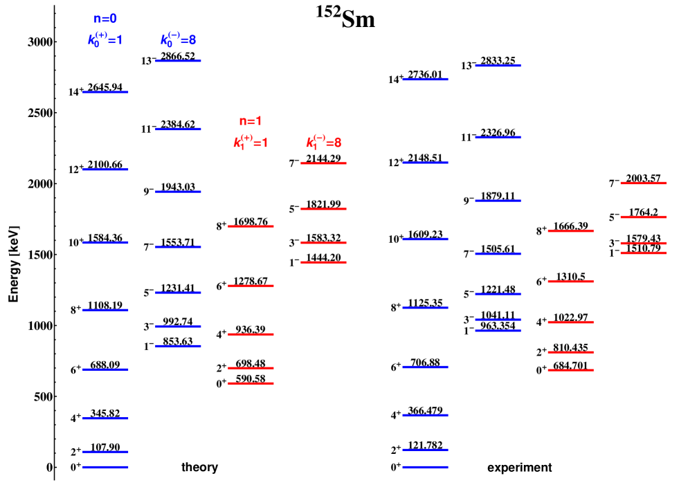
Figure 1: (Color online) Theoretical and experimental alternating-parity bands in ¹⁵²Sm. Data from [34]. The oscillation quantum numbers $n$, $k_{n}^{(+)}$ and $k_{n}^{(-)}$ are given above the theoretical bands.

with $X(I)=[d_{0}+I(I+1)]/2$. $B_{2}$ and $B_{3}$ are effective quadrupole and octupole mass parameters and $C_{2}$ and $C_{3}$ are stiffness parameters for the respective oscillation modes. The quantity ${\mathcal{J}}^{(\mbox{\scriptsize quad+oct})}=(d_{2}\beta_{2}^{2}+d_{3}\beta_{3}^{2})$ can be associated to the moment of inertia of an axially symmetric quadrupole-octupole deformed shape [23] with $d_{2}$ and $d_{3}$ being inertia parameters. The energy potential (4) represents a two-dimensional surface determined by the variables $\beta_{2}$ and $\beta_{3}$ with an angular-momentum-dependent repulsive core at zero deformation (see Fig. 1 in [18]). The parameter $d_{0}$ in the centrifugal factor $X(I)$ characterizes the repulsive core at $I=0$ and determines the overall energy scale for the rotation part of the energy.

The model Hamiltonian (3) represents a D_∞ invariant. Also, it is important to remark that (3) corresponds to a class of axial-symmetric Hamiltonians [9], [10], [13] whose kinetic vibration parts are derived by ignoring the non-axial degrees of freedom (e.g. $\gamma$-vibrations) in a way similar to the approach of Davidov and Chaban [22]. The scalar product in the space of the wave functions (e.g. see Eqs. (2) and (4) in [13]) corresponding to the particular form of the $\beta_{2}$- and $\beta_{3}$-derivatives in (3) is characterized by a unit weight factor, i.e. $\langle\Phi_{2}|\Phi_{1}\rangle=\int\int d\beta_{2}d\beta_{3}\Phi_{2}^{\ast}(\beta_{2},\beta_{3})\Phi_{1}(\beta_{2},\beta_{3})$.

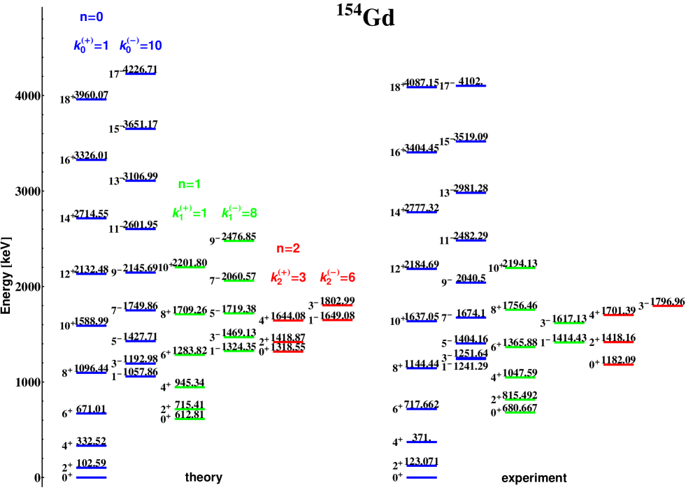
Figure 3: (Color online) The same as in Fig. 1, but for ¹⁵⁴Gd.

If a condition for the simultaneous presence of nonzero coordinates $(\beta_{2}^{\mbox{\scriptsize min}},\beta_{3}^{\mbox{\scriptsize min}})$ of the potential minimum is imposed, the stiffness and inertial parameters are correlated as $d_{2}/C_{2}=d_{3}/C_{3}$ (see Eqs. (3)–(6) in [18]). In this case the potential bottom represents an ellipse in the space of $\beta_{2}$ and $\beta_{3}$ which surrounds the infinite zero-deformation core (see Fig. 3 in [18]). If prolate quadrupole deformations $\beta_{2}>0$ are considered, the system is characterized by oscillations between positive and negative $\beta_{3}$-values along the ellipse surrounding the potential core. By introducing polar-type of curvilinear or, more precise, ellipsoidal variables

$$\eta=\left[\frac{2(d_{2}\beta_{2}^{2}+d_{3}\beta_{3}^{2})}{d_{2}+d_{3}}\right]^{\frac{1}{2}}\qquad\mbox{and}\qquad\phi=\arctan\left({\frac{\beta_{3}}{\beta_{2}}\sqrt{\frac{d_{3}}{d_{2}}}}\right)\ ,$$

such that

$$\beta_{2}=p\eta\cos\phi,\qquad\beta_{3}=q\eta\sin\phi,$$ (5)

with

$$p=\sqrt{\frac{d}{d_{2}}},\qquad q=\sqrt{\frac{d}{d_{3}}}\qquad\mathrm{and}\qquad d=\frac{1}{2}(d_{2}+d_{3}),$$ (6)

the potential (4) appears in the form

$$U_{I}(\eta)=\frac{1}{2}C\eta^{2}+\frac{X(I)}{d\eta^{2}}\ ,$$ (7)

where $C=(d/d_{2})C_{2}=(d/d_{3})C_{3}$.

Further, it is assumed that the quadrupole and octupole modes are represented in the collective motion with the same oscillation frequencies $\omega_{2}=\omega_{3}=\omega$, with

$$\omega=\sqrt{\frac{C_{2}}{B_{2}}}=\sqrt{\frac{C_{3}}{B_{3}}}\equiv\sqrt{\frac{C}{B}}.$$ (8)

The condition (8) imposes certain correlations between the mass, stiffness and inertia parameters of the model Hamiltonian (3), corresponding to a coherent quadrupole-octupole motion of the system. Note that here the term “coherent” is used in the context of the mixing between the quadrupole and octupole degrees of freedom, which is different from the meaning of the same term used in [16]. In this case the Hamiltonian is obtained in a simple form

$$H_{qo} = -\frac{\hbar^{2}}{2B}\left[\frac{\partial^{2}}{\partial\eta^{2}}+\frac{1}{\eta}\frac{\partial}{\partial\eta}+\frac{1}{\eta^{2}}\frac{\partial^{2}}{\partial\phi^{2}}\right]+U_{I}(\eta)\ .$$ (9)

It allows an exact separation of variables in the wave function $\Phi(\eta,\phi)=\psi(\eta)\varphi(\phi)$ with the subsequent equations for $\psi(\eta)$ and $\varphi(\phi)$

$$\frac{\partial^{2}}{\partial\eta^{2}}\psi(\eta)+\frac{1}{\eta}\frac{\partial}{\partial\eta}\psi(\eta)+\frac{2B}{\hbar^{2}}\left[E-\frac{\hbar^{2}}{2B}\frac{k^{2}}{\eta^{2}}-U_{I}(\eta)\right]\psi(\eta) = 0\ ;$$ (10)

$$\frac{\partial^{2}}{\partial\phi^{2}}\varphi(\phi)+k^{2}\varphi(\phi) = 0\ ,$$ (11)

where $k$ is the separation quantum number. Eq. (10) with the potential (7) is similar to the equation for the Davidson potential [24] and has the following analytic solution for the energy spectrum [18]

$$E_{n,k}(I)=\hbar\omega\left[2n+1+\sqrt{k^{2}+bX(I)}\right],$$ (12)

where $\omega$ is defined in (8), $n=0,1,2,...$ and $b=2B/(\hbar^{2}d)$. The quantum numbers $n$ and $k$ have the meaning of “radial” and “angular” oscillation quantum numbers, respectively. The normalized “radial” eigenfunctions $\psi(\eta)$ are obtained in terms of the generalized Laguerre polynomials

$$\psi^{I}_{n,k}(\eta)=\sqrt{\frac{2c\Gamma(n+1)}{\Gamma(n+2s+1)}}e^{-c\eta^{2}/2}(c\eta^{2})^{s}L^{2s}_{n}(c\eta^{2})\ ,$$ (13)

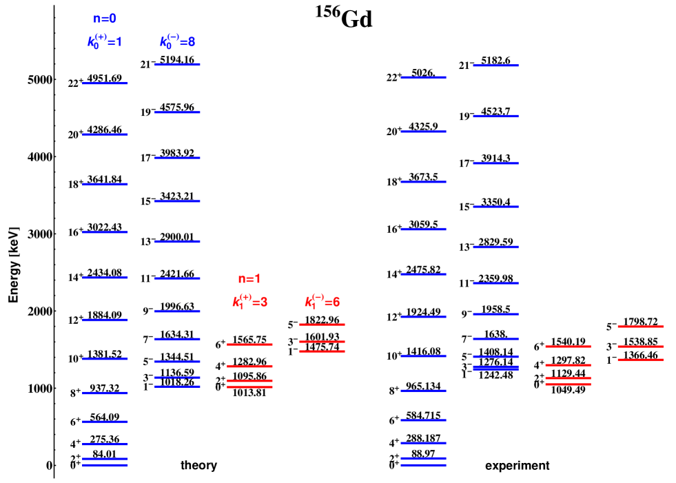
Figure 4: (Color online) The same as in Fig. 1, but for ¹⁵⁶Gd.

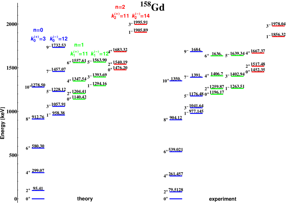
Figure 5: (Color online) The same as in Fig. 1, but for ¹⁵⁸Gd.

with $c=\sqrt{BC}/\hbar$ and $s=(1/2)\sqrt{k^{2}+bX(I)}$. Eq. (11) in the “angular” variable $\phi$ is solved under the boundary condition $\varphi(-\pi/2)=\varphi(\pi/2)=0$. This is equivalent to the consideration of an infinite potential wall at $\beta_{2}=0$ (or $\varphi=\pm\pi/2$). Then one has two identical solutions for $\beta_{2}>0$ and $\beta_{2}<0$. As mentioned above the physical space of the model is taken in the prolate $\beta_{2}>0$ half of the $(\beta_{2},\beta_{3})$-plane. (See Figs. 4 and 5 in [18] and the related text in that reference). Within this half-plane Eq. (11) has two different solutions with positive and negative parities, $\pi=(+)$ and $\pi=(-)$, respectively

$$\varphi_{k}^{+}(\phi) = \sqrt{2/\pi}\cos(k\phi)\ ,\qquad k=1,3,5,...\ ,$$ (14)

$$\varphi_{k}^{-}(\phi) = \sqrt{2/\pi}\sin(k\phi)\ ,\qquad k=2,4,6,...\ .$$ (15)

Note that the square root term in the wave function $\psi^{I}_{n,k}(\eta)$, Eq. (13), differs from the respective term used in Eq. (24) of Ref. [18] by the factor $c$ which is newly included in the numerator. (In [18] the quantity $c$ is denoted by ‘$a$’ which in the case of odd nuclei leads to confusion with the notation for the decoupling factor.) One can easily check that this factor is necessary to normalize $\psi^{I}_{n,k}(\eta)$ to unity. The results for the transition probabilities obtained in [18] are not affected by the missing factor $c$ due to the use of overall scaling factors in Eqs. (46) and (47) of [18].

Since the consideration is restricted to axial deformations only, the projection $K$ of the collective angular momentum on the principal symmetry axis is taken zero. Then the total wave function of the coherent quadrupole-octuple vibration and collective rotation of an even-even nucleus has the form

$$\Psi^{\pi}_{nkIM0}(\eta,\phi)=\sqrt{\frac{2I+1}{8\pi^{2}}}D^{I}_{M\,0}(\theta)\Phi^{\pi}_{nkI}(\eta,\phi)\ ,$$ (16)

where $D^{I}_{M\,0}(\theta)$ is the Wigner function defined according to the phase convention in [25]. Note that due to a different phase convention in some other works, e.g. in [26] and [27], the complex conjugated $D$-function appears in the rotation part. The relations between the different definitions of the $D$-function are given in Table 4.2 in [28]. The quadrupole-octupole vibration part of (16) is

$$\Phi^{\pi}_{nkI}(\eta,\phi)=\psi_{nk}^{I}(\eta)\varphi^{\pi}_{k}(\phi)\ .$$ (17)

The quantum numbers of the quadrupole-octupole vibration function (17) are determined by the requirement for a conservation of the $\mathcal{R}\mathcal{P}$-symmetry of the total wave function (16). ($\mathcal{P}$ is the parity operator and $\mathcal{R}$ represents a rotation by an angle $\pi$ about an axis perpendicular to the intrinsic $z$-axis) The $\mathcal{R}$-symmetry of the rotation function $D^{I}_{M\,0}(\theta)$ is characterized by the factor $(-1)^{I}$, while the action of $\mathcal{P}$ on $\Phi^{\pi}_{nkI}(\eta,\phi)$ gives the factor $\pi=\pm$. Then the conservation of the $\mathcal{R}\mathcal{P}$-symmetry is equivalent to the conservation of the so called simplex quantum number $simplex=\pi(-1)^{I}=1$. This condition imposes a positive parity for the states with even angular momentum, and negative parity for the odd angular momentum states, i.e. one has

$$\Phi^{+}_{nkI}(\eta,\phi) = \psi_{nk}^{I}(\eta)\varphi^{+}_{k}(\phi)\ \mbox{for}\ I=\mbox{even}$$

$$\Phi^{-}_{nkI}(\eta,\phi) = \psi_{nk}^{I}(\eta)\varphi^{-}_{k}(\phi)\ \mbox{for}\ I=\mbox{odd}.$$

It should be noted that the above conditions are in conjunction with the transformation properties of the variables $\eta$ and $\phi$ in (17) under the rotation $\mathcal{R}$ ($\eta$ is invariant, while $\phi$ changes in sign) so that together with the simplex conservation condition the total wave function (16) appears to be an D_∞ invariant as it should be due to the axial symmetry.

The structure of the energy spectrum is determined by the oscillator quantum numbers $n$ (“radial”) and $k$ (“angular”) in Eq. (12). Since according to Eqs. (14) and (15) $k$ obtains different values for the states with opposite parity the energy sequences with even and odd angular momenta corresponding to a given $n$ appear shifted to each other, i.e. a parity shift effect is observed. In [18] it was supposed that the $g$-band and the lowest negative-parity band belong to a $n=0$ set with $k=k^{(+)}=1$ for $g$ and $k=k^{(-)}=2$ for the negative-parity band. In the present work the model scheme is extended through the following three suppositions.

i) The energy spectrum determined by the coherent axial quadrupole-octupole vibrations and rotations consists of couples of level-sequences with opposite parity. The sequences in each couple are characterized by the same value of the quantum number $n=0,1,2,...$ and by different values of $k$, $k=k_{n}^{(+)}=1\,\mbox{or}\,3\,\mbox{or}\,5\,\mbox{or}\,...$ for the even-$I$ sequence, and $k=k_{n}^{(-)}=2\,\mbox{or}\,4\,\mbox{or}\,6\,\mbox{or}\,...$ for the odd-$I$ sequence.

ii) The lowest values of the “radial” quantum number $n$ correspond to the lowest alternating parity bands, with $n=0$ being the yrast band, $n=1$ corresponding to the next non-yrast alternating parity structure and so on. The values of the “angular” quantum number $k$ are not restricted and should only satisfy the parity condition in i). The particular values of $k_{n}^{(+)}$ and $k_{n}^{(-)}$ can be determined so as to reproduce the experimentally observed parity shift in the set of levels with a given $n$.

iii) Due to the coherent interplay between the $\beta_{2}$ and $\beta_{3}$ variables in the oscillation motion, the excited $\beta$-bands in even-even nuclei can be interpreted as the positive-parity counterparts of higher negative-parity sequences, or as the members of non-yrast alternating-parity bands.

Based on the above assumptions the extended alternating-parity spectrum of an even-even nucleus can be considered in the following form.

Yrast alternating-parity set $(n=0)$: unites the $g$-band $(k=k_{0}^{(+)})$ $I_{\nu}^{\pi}=0_{1}^{+},2_{1}^{+},4_{1}^{+},6_{1}^{+},...$ with the first negative-parity band denoted here as $n1$ $(k=k_{0}^{(-)})$ $I_{\nu}^{\pi}=1_{1}^{-},3_{1}^{-},5_{1}^{-},...;$

First non-yrast set $(n=1)$: unites the first $\beta$-band denoted by $b1$ $(k=k_{1}^{(+)})$ $I_{\nu}^{\pi}=0_{2}^{+},2_{2}^{+},4_{2}^{+},...$ with the second negative-parity band denoted by $n2$ $(k=k_{1}^{(-)})$ $I_{\nu}^{\pi}=1_{2}^{-},3_{2}^{-},5_{2}^{-},...;$

Second non-yrast set $(n=2)$: unites the second $\beta$-band $b2$ $(k=k_{2}^{(+)})$ $I_{\nu}^{\pi}=0_{3}^{+},2_{3}^{+},4_{3}^{+},...$ with the third negative-parity band $n3$ $(k=k_{2}^{(-)})$ $I_{\nu}^{\pi}=1_{3}^{-},3_{3}^{-},5_{3}^{-},...$, and so on, higher non-yrast sequences, where $\nu=1,2,3,...$ is the consequent number of the appearance of a state with a given angular momentum. Also, it is convenient to use the band labels introduced above to denote the different excited states as for example $2_{g}^{+}$, $1_{n1}^{-}$, $0_{b1}^{+}$, $1_{n2}^{-}$ etc.

Obviously the above model scheme makes no claim to exhaust the entire collective spectrum but rather provides a tool to identify the extent to which the considered quadrupole-octupole motion can influence the excited band structures in even-even nuclei. In the end of this section, it should be remarked that the extension of the model to higher energy levels, together with assumption ii), which releases $k$ from the fixed values $k^{(+)}=1$ and $k^{(-)}=2$ (originally imposed in [18] for the yrast case), now requires a new readjustment of the model parameters.

3 Transition probabilities in the non-yrast quadrupole-octupole states

As the B(E1) and B(E3) reduced transition probabilities are known to provide a sensitive test for the structure of the alternating-parity sequences it is of special importance to examine their behaviour in the non-yrast part of the spectrum. The basic CQOM concept for the electromagnetic transitions has been given in [18]. Here the formalism is modified so as to describe B(E1), B(E2) and B(E3) reduced transition probabilities in the higher lying alternating-parity bands along with the extended treatment of the model energy quantum numbers. A more essential modification is related to a generalization of the angular part of the electric transition operators dictated by the complicated quadrupole-octupole shape density distribution inherent for the coherent motion mode (see below). In addition the E1-E3 charge factors are treated explicitly and the model parameters $p$ and $q$ (6) providing information about the potential shape are considered without including them into scaling constants.

The reduced transition probability for an electric transition with a given multipolarity $\lambda$ between model states (16) with $n=n_{i}$, $k=k_{i}$, $I=I_{i}$ and $n=n_{f}$, $k=k_{f}$, $I=I_{f}$ is

$$B(E\lambda;n_{i}k_{i}I_{i}\rightarrow n_{f}k_{f}I_{f})=\frac{1}{2I_{i}+1}\sum_{M_{i}M_{f}\mu}\left|\left\langle\Psi^{\pi_{f}}_{n_{f}k_{f}I_{f}M_{f}0}(\eta,\phi)|\mathcal{M}_{\mu}(E\lambda)|\Psi^{\pi_{i}}_{n_{i}k_{i}I_{i}M_{i}0}(\eta,\phi)\right\rangle\right|^{2}.$$ (18)

The operators for electric E1, E2 and E3 transitions have the following general form

$$\mathcal{M}_{\mu}(E\lambda)=\sqrt{\frac{2\lambda+1}{4\pi(4-3\delta_{\lambda,1})}}\hat{Q}_{\lambda 0}D^{\lambda}_{0\mu},\ \ \lambda=1,2,3,\ \ \mu=0,\pm 1,...,\pm\lambda.$$ (19)

The vibration parts of these operators are given up to the first order of $\beta_{2}$ and $\beta_{3}$, for E2 and E3, and in second order, for E1, as

$$\hat{Q}_{10} = M_{1}\beta_{2}\beta_{3}$$ (20)

$$\hat{Q}_{\lambda 0} = M_{\lambda}\beta_{\lambda},\ \ \ \ \lambda=2,3.$$ (21)

The electric charge factors $M_{\lambda}$ $(\lambda=2,3)$ are taken as [29]

$$M_{\lambda}=\frac{3}{\sqrt{(2\lambda+1)\pi}}ZeR_{0}^{\lambda},\qquad\lambda=2,3\ ,$$ (22)

where $R_{0}=r_{0}A^{1/3}$, $r_{0}\approx 1.2$ fm, $Z$ is the proton number, and $e$ is the electric charge of the proton. The charge factor $M_{1}$ is taken according to the droplet model concept [30]-[32] in the form [10]

$$M_{1}=\frac{9AZe^{3}}{56\sqrt{35}\pi}\left(\frac{1}{J}+\frac{15}{8QA^{\frac{1}{3}}}\right),$$ (23)

where the quantities $J$ and $Q$ are related to the volume and surface symmetry energy, respectively and their values are assumed in the limits $25\lesssim J\lesssim 44$ MeV and $17\lesssim Q\lesssim 70$ MeV [33] (see also the values below Eq. (79) in [10]). In the present work fixed average values of these quantities $J=35$ MeV and $Q=45$ MeV are used for all considered nuclei. One should remark that so far there is no unique approach to estimate the factor $M_{1}$. Therefore, here in (23) the proton charge $e$ is replaced by an effective charge $e^{1}_{eff}$ which is considered as an adjustable parameter and can be different from one. Note that to obtain the B(E1) transition probabilities in the units $e^{2}\cdot\mbox{fm}^{2}$, and subsequently in Weisskopf units one has to take into account that $e^{2}=1.4399764\,\mbox{MeV}\cdot\mbox{fm}$ [or $e^{6}/\mbox{MeV}^{2}=(1.4399764)^{2}e^{2}\cdot\mbox{fm}^{2}$] which leads to an additional multiplication factor 1.4399764 in (23) when numerical values are produced.

In the space of the ellipsoidal coordinates (5), (6) one has

$$\hat{Q}_{10} = M_{1}pq\eta^{2}\cos\phi\sin\phi$$ (24)

$$\hat{Q}_{20} = M_{2}p\eta\cos\phi$$ (25)

$$\hat{Q}_{30} = M_{3}q\eta\sin\phi.$$ (26)

The definitions of the operators (20)–(21) and (24)–(26) originally correspond to a situation in which the nuclear shape is characterized by fixed values of the deformation parameters $\beta_{2}$ and $\beta_{3}$. In this case the density distribution of the collective state is characterized by a single maximum in the space of $\beta_{2}$ and $\beta_{3}$. In the case of the model potential (4) taken with an elliptic bottom the density distribution can be characterized by more than one maximum. Indeed, the density of the model state (17) is characterized by a different number of maxima depending on the quantum number $k$. This feature is a result of the assumed soft quadrupole–octupole mode. It is illustrated graphically in Appendix A, where the density distribution of the state (17) in the space of the quadrupole-octupole deformations is plotted for different $k$-values at $n=0$ after transforming the wave function $\Phi^{\pi}_{nkI}$ in the ($\beta_{2}$,$\beta_{3}$) variables. It is seen that for $\beta_{2}>0$ the number of maxima is equal to $k$ and by analogy with the acoustics may be interpreted as the number of “overtones” which characterize the coherent collective oscillations of the system. Thus, it appears that the transition operators should connect states with different numbers of maxima (or overtones). In the space of ellipsoidal variables the positions of the maxima are determined by the angular variable $\phi$. On the other hand the original operators (24)–(26) do not take into account the presence of multiple maxima in the shape density distributions of the different states. One particular effect due to this circumstance is that the integrals over the angular part of (26), $\sin\phi$, vanish when the difference between the $k$ numbers of the initial and final states is larger than a unit and the respective B(E3) transition probabilities vanish too. This limitation is removed if the operators are generalized appropriately. The most general forms of the angular parts of the operators corresponding to the first orders of $\beta_{2}$ and $\beta_{3}$ according to (25) and (26) can be sought in terms of a Fourier expansion with respect to $\phi$ through the replacements

$$\cos\phi\rightarrow A_{20}(\phi)\equiv\sum_{k=1}^{\infty}a^{(k)}_{20}\cos(k\phi),\qquad\sin\phi\rightarrow A_{30}(\phi)\equiv\sum_{k=1}^{\infty}a^{(k)}_{30}\sin(k\phi),$$ (27)

where the expansion coefficients should be chosen so as to provide an appropriate convergence. A choice made here for both type of coefficients is $a^{(k)}=1/k$ for which the above expansions can be obtained in analytic form

$$A_{20}(\phi) = \sum_{k=1}^{\infty}\frac{\cos(k\phi)}{k}=-\frac{1}{2}[\ln 2+\ln(1-\cos\phi)]$$ (28)

$$A_{30}(\phi) = \sum_{k=1}^{\infty}\frac{\sin(k\phi)}{k}=\frac{\pi-\phi}{2}+\pi\mbox{Floor}\left(\frac{\phi}{2\pi}\right),$$ (29)

where the Floor function maps a real number to the largest previous integer. Then the angular part of the second order operator (24) can be generalized in an obvious way

$$\cos\phi\sin\phi\rightarrow A_{10}(\phi)\equiv A_{20}(\phi)A_{30}(\phi)=\sum_{m=1}^{\infty}\sum_{n=1}^{\infty}\frac{\cos(m\phi)}{m}\frac{\sin(n\phi)}{n}.$$ (30)

Note that the first terms of the above expansions represent the original angular parts in (24)–(26). So, the new angular operators (28)–(30), which are extensions of the old ones, provide a connection between states whose “dynamical” deformations (i.e. the probability distribution in the deformation space) are characterized by the co-existence of a large number of maxima. These specific shape properties of the system are due to the assumed coupling between quadrupole and octupole degrees of freedom. Now the operators (24)–(26) are redefined as

$$\hat{Q}_{10}(\eta,\phi) = M_{1}pq\eta^{2}A_{10}(\phi)$$ (31)

$$\hat{Q}_{20}(\eta,\phi) = M_{2}p\eta A_{20}(\phi)$$ (32)

$$\hat{Q}_{30}(\eta,\phi) = M_{3}q\eta A_{30}(\phi).$$ (33)

After carrying out the integration over the rotation part in (18) one obtains

$$B(E\lambda;n_{i}k_{i}I_{i}\rightarrow n_{f}k_{f}I_{f})=\frac{2\lambda+1}{4\pi(4-3\delta_{\lambda,1})}\langle I_{i}0\lambda 0|I_{f}0\rangle^{2}R_{\lambda}^{2}(n_{i}k_{i}I_{i}\rightarrow n_{f}k_{f}I_{f}),$$ (34)

which involves the squares of the Clebsch-Gordan coefficient and the matrix element of the electric multipole operators (31)-(33) between the quadrupole-octupole vibration wave functions (17)

$$R_{\lambda}(n_{i}k_{i}I_{i}\rightarrow n_{f}k_{f}I_{f})=\left\langle\Phi^{\pi_{f}}_{n_{f}k_{f}I_{f}}(\eta,\phi)|\hat{Q}_{\lambda 0}|\Phi^{\pi_{i}}_{n_{i}k_{i}I_{i}}(\eta,\phi)\right\rangle.$$ (35)

By further separating the integrations over the “radial” variable $\eta$ and the “angular” variable $\phi$ in (35) according to (17) one obtains

$$R_{1}(n_{i}k_{i}I_{i}\rightarrow n_{f}k_{f}I_{f}) = M_{1}pqS_{2}(n_{i},I_{i};n_{f},I_{f})I_{1}^{\pi_{i},\pi_{f}}(k_{i},k_{f})$$ (36)

$$R_{2}(n_{i}k_{i}I_{i}\rightarrow n_{f}k_{f}I_{f}) = M_{2}pS_{1}(n_{i},I_{i};n_{f},I_{f})I_{2}^{\pi_{i},\pi_{f}}(k_{i},k_{f})$$ (37)

$$R_{3}(n_{i}k_{i}I_{i}\rightarrow n_{f}k_{f}I_{f}) = M_{3}qS_{1}(n_{i},I_{i};n_{f},I_{f})I_{3}^{\pi_{i},\pi_{f}}(k_{i},k_{f}),$$ (38)

where

$$S_{1}(n_{i},I_{i};n_{f},I_{f}) = \int_{0}^{\infty}d\eta\psi_{n_{f}}^{I_{f}}(\eta)\eta^{2}\psi_{n_{i}}^{I_{i}}(\eta)$$ (39)

$$S_{2}(n_{i},I_{i};n_{f},I_{f}) = \int_{0}^{\infty}d\eta\psi_{n_{f}}^{I_{f}}(\eta)\eta^{3}\psi_{n_{i}}^{I_{i}}(\eta),$$ (40)

and

$$I_{\lambda}^{\pi_{i},\pi_{f}}(k_{i},k_{f}) = \frac{2}{\pi}\int_{-\frac{\pi}{2}}^{\frac{\pi}{2}}A_{\lambda 0}(\phi)\varphi^{\pi_{f}}_{k_{f}}(\phi)\varphi^{\pi_{i}}_{k_{i}}(\phi)d\phi,\ \ \ \lambda=1,2,3.$$ (41)

The integrals over $\eta$, (39) and (40), involve the “radial” wave functions (13). Analytic expressions for these integrals are given in Appendix B. The integrals over $\phi$ (41) involve the “angular” wave functions (14) and/or (15). The explicit forms of these integrals with the relevant parities $\pi_{i}$ and $\pi_{f}$ are given in Appendix C.

From the generalized definitions (31)-(33) of the operators $\hat{Q}_{\lambda 0}$ it is seen that the inertial factors $p$, $q$ and their product $pq$ defined through Eq. (6) are not included in any scaling factors, as done in Ref. [18] and can be considered as model parameters. Actually, $p$ and $q$ are not independent. From (6) it can be easily seen that $1/p^{2}+1/q^{2}=2$. Then $q$ can be expressed by $p$ as

$$q=\frac{p}{\sqrt{2p^{2}-1}},\qquad\mathrm{with}\qquad p>\frac{1}{\sqrt{2}}\approx 0.7071.$$ (42)

The inequality in (42) corresponds to the condition $d_{2}<2d$. Analogically one can express $p$ by $q$ with the condition $d_{3}<2d$. (Note that for $p=1$ one has $q=1$ and $pq=1$.) Here the adjustable parameter is chosen to be $p$. It should be noted that with the involvement of the new parameter $p$ the scaling factors in Eqs. (46) and (47) of Ref. [18] are not considered anymore and the charge factors $M_{2}$ and $M_{3}$ are directly calculated in (22). Also the charge factor $M_{1}$ is directly calculated in (23), but with the effective charge $e^{1}_{eff}$ being adjusted to determine the correct scale of the B(E1) transition probabilities with respect to B(E2). From another side the parameter $p$ determines the relative scale between B(E2) and B(E3). It is interesting to remark that $p$ does not play any role if the model energy levels are fitted without taking into account transition probabilities. However, in this case there is an ambiguity in the choice of the inertial parameters $d_{2}$ and $d_{3}$. This is seen by the following relations between the parameters of the potential (4) and the fitting parameters $\omega$ and $b$, imposed by the coherent condition (8)

$$C_{2} = \frac{\omega^{2}b}{2}d_{2},\qquad C_{3}=\frac{\omega^{2}b}{2}d_{3}$$ (43)

$$B_{2} = \frac{b}{2}d_{2},\qquad\ \ \ B_{3}=\frac{b}{2}d_{3},$$ (44)

in which $d_{2}$ and $d_{3}$ are not determined. (The parameter $d_{0}$ does not enter these relations.) This means that for a given set of parameters $\omega$, $b$ and $d_{0}$ the energy spectrum corresponds to an infinite number of potential shapes with different eccentricities of the ellipsoidal bottom. Now, after determining the parameters $p$ and $c$ with respect to transition data one gets

$$d_{2}=\frac{d}{p^{2}},\qquad d_{3}=(2p^{2}-1)\frac{d}{p^{2}},\qquad\mathrm{with}\qquad d=\frac{2c}{\omega b}.$$ (45)

Thus for given values of the parameters $\omega$, $b$, $c$ and $p$ the original parameters $B_{2}$, $B_{3}$, $C_{2}$, $C_{3}$, $d_{2}$ and $d_{3}$ of potential (4) are fixed, and given additionally $d_{0}$, its form is unambiguously determined.

4 Numerical results and discussion

The extended CQOM formalism was applied to several nuclei, namely ^152,154Sm, ^154,156,158Gd, ²³⁶U and ¹⁰⁰Mo, in which one or two non-yrast alternating-parity bands can be constructed by the experimentally observed $\beta$ and higher-lying negative-parity levels. In these nuclei a number of data on E1 and/or E3 transitions are available providing the possibility to test the complete model scheme. In all selected nuclei the experimental data [34] provide well determined yrast and first non-yrast alternating-parity bands except for ¹⁰⁰Mo where the structure of the non-yrast band is proposed here on the basis of the model analysis (see below). In three of the nuclei, ¹⁵⁴Sm, ¹⁵⁴Gd and ¹⁵⁸Gd second excited (non-yrast) alternating-parity bands are additionally considered. The structure of these bands is not clearly determined in the experimental data. Therefore, the model description and prediction provides a possible interpretation of the respective experimental levels. In this meaning the present description not only provides a test for the CQOM model scheme, but also suggests a possible classification of some highly non-yrast excited states whose interpretation in the experimental data bases is not unambiguous.

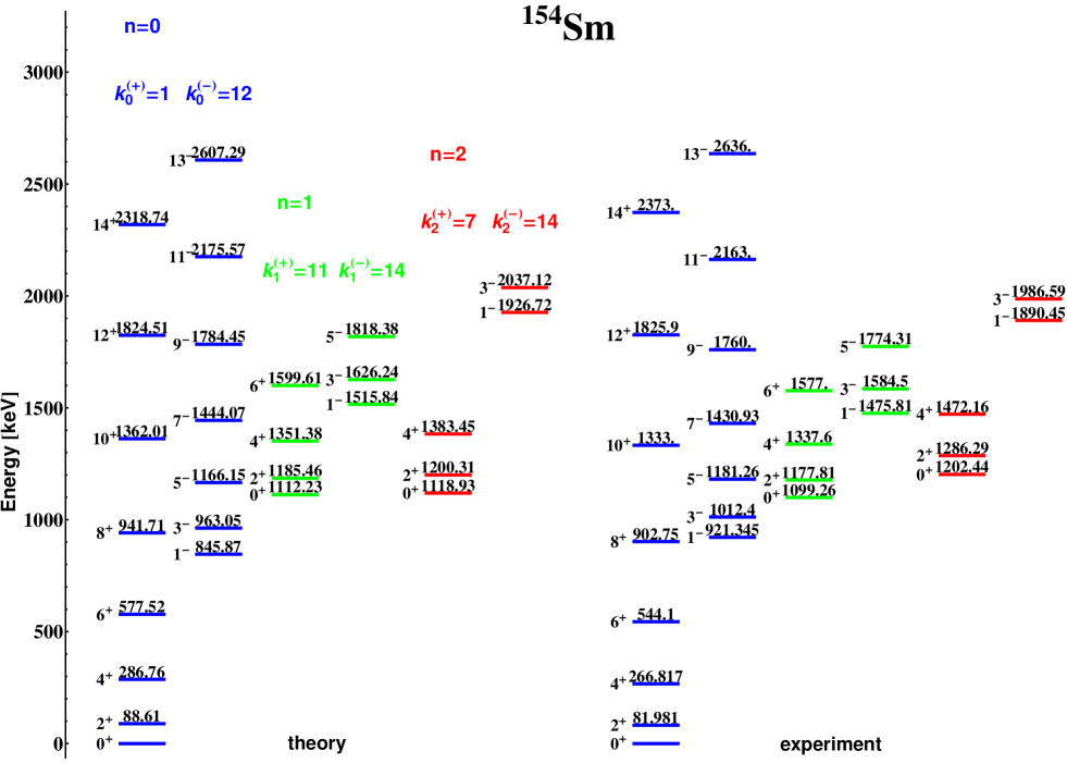
Figure 2: (Color online) The same as in Fig. 1, but for ¹⁵⁴Sm.

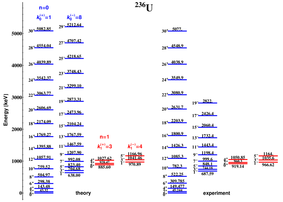
Figure 6: (Color online) The same as in Fig. 1, but for ²³⁶U.

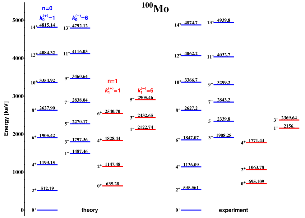
Figure 7: (Color online) The same as in Fig. 1, but for ¹⁰⁰Mo.

The model description is obtained by taking the theoretical energy levels $\tilde{E}_{n,k}(I)=E_{n,k}(I)-E_{0,k_{0}^{(+)}}(0)$ from Eq. (12). The parameters $\omega$, $b$, $d_{0}$, $c$, $p$ and the effective charge $e^{1}_{eff}$ have been adjusted by simultaneously taking into account experimental data on the energy bands and the available B(E1)-B(E3) transition probabilities. The parameter values obtained in the considered nuclei are given in Table 1. The resulting values of the original Hamiltonian parameters in (3) and (4) are given in Table 2. For each nucleus the calculations are performed in a net over the values of the “angular” quantum numbers $k$ with appropriate parity in the limits $1\leq k\leq 20$. In all nuclei sets of values for the $k$-quantum numbers providing the best model description of both, energies and reduced transition probabilities, are obtained. These values are given in Figures 1–7 where the theoretical and experimental energy levels of the considered nuclei are compared. The theoretical and experimental values of the B(E1), B(E2) and B(E3) transition probabilities are compared in Table 3. Model predictions for some not yet observed transitions are also given there.

The results in Figs. 1–7 show that the model scheme correctly reproduces the structure of the alternating-parity spectra in the considered nuclei with a reasonably good agreement between the theoretical and experimental energy levels. The correct reproduction of the mutual displacement of the different positive and negative parity sequence is related to the involvement of $k$ quantum number values larger than 1 and 2. On the other hand the determination of the $k$-values is strongly dictated by the interband transitions between the positive- and negative- parity levels as well as by the transitions between the different alternating-parity sequences. The above remarks explain why for the nuclei ¹⁵²Sm and ¹⁵⁴Gd new sets of $k$-quantum numbers appear together with renormalized values of the fitting parameters compared to the previous descriptions limited to the yrast bands [18] (see below). One should remark that at the same time the main (radial) oscillator quantum number $n$ is uniquely determined, $n=0$ for the yrast sequence, $n=1$ for the first excited alternating parity band and so on, as explained in the end of Sec. 2.

In ¹⁵²Sm the yrast band is described together with the first excited band (see Fig. 1). The calculations provide two identical couples of $k$ values $(k^{(+)}=1,k^{(-)}=8)$ for each band. Thus it is seen that $k^{(-)}$ obtains a value larger than the lowest even value $2$ considered in [18]. From Table 3 one can see that with this configuration of $k$-numbers the model fairly good reproduces the data [35] on the B(E2) intraband transition probabilities in the ground-state band ($g$) and on the B(E1) probabilities for transitions between the $g$- and the first negative-parity band ($n1$). Some interband $E2$ transitions between the $g$- and the first $\beta$-band ($b1$), as $2_{b1}^{+}\rightarrow 2_{g}^{+}$ and $4_{b1}^{+}\rightarrow 4_{g}^{+}$ are also well described, while others like $4_{b1}^{+}\rightarrow 6_{g}^{+}$ are overestimated. The calculated intraband transitions in the $b1$-band are in rough agreement with the experimental data, while the $E1$ intraband transition $1_{n1}^{-}\rightarrow 2_{b1}^{+}$ is overestimated by an order. The E3 transition probability B$(E3;3_{n1}^{-}\rightarrow 0_{g}^{+})=14$ W.u. [36] is exactly reproduced due to the adjustable parameter $p$ which determines the factor $q$ in (38) according to Eq. (42). This allows one to predict other E3 transitions like $1_{n1}\rightarrow 4_{g}$ and other similar transitions between the $b1$-band and the second negative-parity band ($n2$) as shown in Table 3. Although not all theoretical transition probabilities are in strict agreement with the experimental data it is seen that the model scheme correctly takes into account the different scales of the various kinds of probabilities. A similar behaviour of transition probabilities is observed in the other considered nuclei.

In ¹⁵⁴Sm totally three alternating-parity bands are considered as seen from Fig. 2. The positive-parity states of the second excited band are interpreted in [34] as members of a second $K^{\pi}=0^{+}$ band, or of a second $\beta$-band $(b2)$. The respective negative-parity levels are selected in the present work among levels for which there is no interpretation given in [34]. Here they form a third negative-parity band $(n3)$. From Table 3 it is seen that the intraband B(E2) transition probabilities in the $g$-band of this nucleus are reasonably well described up to $I=10$, while the B$(E2;12_{g}^{+}\rightarrow 10_{g}^{+})$ value is considerably overestimated. The B(E1) probabilities between the $n1$- and $g$-bands are also well described. The theoretical interband transition value B$(E2;0_{b1}^{+}\rightarrow 2_{g}^{+})$ is by an order smaller than the experimental one. For the other similar E2 transitions like $2_{b1}^{+}\rightarrow 0_{g}^{+}$ the theoretical values are obtained below the upper limits given for the respective experimental data [35].

In ¹⁵⁴Gd, again, three alternating-parity bands are considered. The model description is given in Fig. 3. Here, the second non-yrast band is constructed by the second excited $K^{\pi}=0^{+}$ band and a $3^{-}$ state with energy 1796.96 keV [34]. Although the latter is interpreted in [34] as a member of a $K^{\pi}=2^{-}$ octupole band it reasonably fits the present scheme as a member of an $n3$-sequence. In this nucleus the B(E1)–B(E3) transition probabilities are also reasonably described with the largest discrepancies between the theory and experiment, about a factor of 2, being observed for the E2 transitions $2_{b1}^{+}\rightarrow 0_{b1}^{+}$ and $0_{b1}^{+}\rightarrow 2_{g}^{+}$ (see Table 3). Note that here the theoretical B(E1) value for the interband transition B$(E1;1_{n1}^{-}\rightarrow 2_{b1}^{+})=0.0064$ W.u. is obtained close to the experimental one, $0.0099$ W.u.

In ¹⁵⁶Gd two alternating-parity bands, the yrast and first excited, are considered (see Fig. 4). The B(E2) and B(E1) transition probabilities between the members of the $g$-, $b1$- and $n1$-bands are well described with a few exceptions as in the transitions $4_{b1}^{+}\rightarrow 2_{b1}^{+}$ and $4_{b1}^{+}\rightarrow 2_{g}^{+}$ for which the B(E2)-values are underestimated with respect to the experiment by a factor of about two and an order, respectively (see Table 3). On the other hand the model predictions for the B(E1) transition probabilities between the second negative-parity band $n2$ and the $g$-band suggest $2$-$3$ orders of magnitude in suppression compared to experimental data.

In ¹⁵⁸Gd, three alternating-parity bands are considered (see Fig. 5). Similarly to ¹⁵⁴Gd the $1^{-}$ and $3^{-}$ states included in the second excited band enter the present model scheme as $n3$-members, while in [34] they are interpreted as members of a $K^{\pi}=1^{-}$ octupole band. For this nucleus, quite a large number of data on B(E1) and B(E2) transition probabilities are available [35]. One should remark that compared to the other considered rare-earth nuclei ¹⁵⁸Gd is closer situated to the region of pronounced rotation collectivity. From Table 3 it is seen that the theoretical intraband B(E2) probabilities in the $g$-band of ¹⁵⁸Gd faster increase with the angular momentum compared to the experimental data. On the other hand six experimental B(E1) values for the transitions between the $g$- and the $n1$-bands are described quite well. It is remarkable that an experimental estimation for a E1 transition between the $n2$- and $b1$-band is available with B$(E1;3_{n2}^{-}\rightarrow 2_{b1}^{+})>0.00035$ W.u. This circumstance is in a conjunction with the model assumption about the quadrupole-octupole coupling of both bands. The model description predicts for this probability a smaller value of 0.00011 W.u., which is of the same order as the B(E1) values connecting the $g$- and $n1$-bands. Further, model prediction values for similar B(E1) transition probabilities as B$(E1;1_{n2}^{-}\rightarrow 0_{b1}^{+})=8\times 10^{-5}$ W.u. and B$(E1;1_{n2}^{-}\rightarrow 2_{b1}^{+})=0.0002$ W.u. are given in Table 3. Also there one can find available experimental estimations for intraband transition probabilities like B$(E2;5_{n1}^{-}\rightarrow 3_{n1}^{-})=369$ W.u. and B$(E2;3_{n2}^{-}\rightarrow 1_{n2}^{-})>1600$ W.u. which are underestimated by the theory. In addition, a number of B(E1) transition probabilities from $b1$- to $n1$-, from $n2$- to $g$- and from $b2$- to $n1$- and $n2$-bands are generally underestimated by one or two orders of magnitude.

In ²³⁶U two alternating-parity bands, the yrast and first excited, are considered (see Fig. 6). This nucleus was selected because of the possibility to examine two observed reduced probabilities for E3 transitions, namely B$(E3;1_{n1}^{-}\rightarrow 4_{g})=62$ W.u. [35] and B$(E3;3_{n1}\rightarrow 0_{g})=22.9$ W.u. [36]. From Table 3 it is seen that the first one is exactly reproduced. The second one is underestimated by the theoretical value, $15$ W.u., which is still reasonably close to the experiment. For the B(E2) transition probabilities within the $g$-band the description is good as overall up to a quite high angular momentum $I=26$. The experimental B(E1) value for the transition $1_{n1}^{-}\rightarrow 0_{g}^{+}$ is exactly reproduced because of the use of the effective charge. This allows one to predict other B(E1) transition probabilities in the described spectrum which are given in Table 3.

In ¹⁰⁰Mo the experimentally observed $2_{3}^{+}$ state with energy $1463.9$ keV is considered in [34] as a possible member of a $\beta$-band. However, the present scheme suggests that the $2^{+}$ state belonging to this band should lie essentially lower. The calculations show that the experimental $2_{2}^{+}$ state with energy $1063.78$ keV considered in [34] as a possible member of a $\gamma$-band is more appropriate as a $\beta$-band member. The result in Fig. 7 shows that if this state is included in the $b1$-band (in the present notations) a non-yrast alternating-parity sequence can be constructed and reasonably well described by taking three additional states, namely $1^{-}$ at $2156$ keV, $3^{-}$ at $2369.6$ keV and $4^{+}$ at $1771.4$ keV from the set of available but not interpreted data for ¹⁰⁰Mo [34]. The observed B(E1)-B(E3) transition probabilities are reasonably described as seen from Table 3. The main discrepancy between the theory and the experiment, a factor of 5, is obtained for the E2 intraband transition $2_{b1}^{+}\rightarrow 0_{b1}^{+}$.

The following comments on the model results can be made here. The parameters of the fits shown in Table 1 reflect the common collective structure of the various energy sequences ($g$, $b1$, $b2$, $n1$, $n2$, $n3$) in a given nucleus, while the sets of $k$ values given in Figs 1-7 reflect their mutual dispositions. Note that the parameters for ¹⁵²Sm and ¹⁵⁴Gd are essentially renormalized compared to the fits of the yrast band only [18]. As seen from Table 1 the parameters $\omega$ and $b$, which are responsible for the rotation-vibration behaviour of the different sequences, vary relatively smoothly between the different nuclei. The parameter $d_{0}$, which is responsible for the shape of the potential at zero angular momentum, shows more pronounced differences in its values, especially for the nuclei from different regions as ²³⁶U and ¹⁰⁰Mo. Also, the parameter $c$, which determines the overall scale for the transition probabilities in the “radial” integrals, considerably varies, while the parameter $p$ which is related to the quadrupole and octupole contributions to the moment of inertia changes quite smoothly. It is remarkable that in three nuclei, ¹⁵²Sm, ¹⁵⁴Sm and ¹⁵⁴Gd, the effective charge for the E1 transitions is practically unit which means that there is no need for this parameter to describe them. In ¹⁵⁶Gd it is still close to 1, while in the other three nuclei its need for the model description is already essential.

By using the relations (44) and (45) between the model parameters in ellipsoidal coordinates and the parameters of the original Hamiltonian, (3) with (4), one can obtain the latters from the values given in Table 1. Subsequently one can obtain the semi-axes (sa) $\beta_{2}^{\mbox{\scriptsize sa}}$ and $\beta_{3}^{\mbox{\scriptsize sa}}$ of the ellipsoidal potential bottom in the space of the quadrupole–octupole variables given by

$$\beta_{\lambda}^{\mbox{\scriptsize sa}}(I)=[2X(I)/d_{\lambda}C_{\lambda}]^{1/4},\qquad\lambda=2,3.$$ (46)

(For more details see the text after Eqs. (3) and (4) of [18].) The resulting values of the parameters $B_{2}$, $B_{3}$, $C_{2}$, $C_{3}$, $d_{2}$, $d_{3}$ and the semi-axes are given in Table 2. Note that in the present work they are not directly adjusted, but obtained as a result of the adjustment of the parameters $\omega$, $b$, $d_{0}$, $c$, $p$, and $e^{1}_{eff}$. As such they only give a rough estimation about the order of the potential parameters and its shape. One can see that for ^152,154Sm and ^154,156Gd these parameters vary relatively smoothly, while for the remaining three nuclei they show some essential fluctuations. The values of the $\beta_{2}^{\mbox{\scriptsize sa}}$ semi-axis are obtained close to the known values of the static quadrupole deformations in these nuclei while the values of the octupole semi-axis $\beta_{3}^{\mbox{\scriptsize sa}}$ appear considerably larger. This result is correlated with the larger values of the quadrupole stiffness parameters $C_{2}$ compared to the values of $C_{3}$. Hence the present parameters correspond to a vibration motion with a larger softness of the system with respect to the octupole mode compared to the quadrupole one. A closer look on the formalism shows that the ratio between both semi-axes is related to the matrix elements of the quadrupole and octupole electric multipole operators (32) and (33). By using (43), (45) and (42) in (46) one finds that

$$\frac{\beta_{3}^{\mbox{\scriptsize sa}}}{\beta_{2}^{\mbox{\scriptsize sa}}}=\frac{q}{p}=\frac{1}{\sqrt{2p^{2}-1}}.$$ (47)

It is seen that the ratio $\beta_{3}^{\mbox{\scriptsize sa}}/\beta_{2}^{\mbox{\scriptsize sa}}$ depends on the inertia factors $p$ and $q$, Eq (6), which determine the strength of the E2 and E3 transitions, respectively. This ratio is less than 1 for $p>1$ $(q<1)$. It can be easily checked that to obtain $\beta_{3}^{\mbox{\scriptsize sa}}/\beta_{2}^{\mbox{\scriptsize sa}}<1$ one has to introduce an additional scaling constant, $c_{3}$, having the meaning of an effective charge for the octupole mode. Then the octupole charge factor is renormalized as $M_{3}^{\prime}=c_{3}M_{3}$. The numerical analysis shows that if $c_{3}$ is chosen in the limits $2\leq c_{3}\leq 4$ the parameter $p$ is renormalized so that $q\rightarrow q/3$ and the same theoretical levels and transition probabilities are obtained with $\beta_{3}^{\mbox{\scriptsize sa}}<\beta_{2}^{\mbox{\scriptsize sa}}$ in correspondence to the usually observed values of the deformation parameters $\beta_{2}$ and $\beta_{3}$. For example if $c_{3}=4$ one obtains the following set of renormalized parameters for ¹⁵⁴Gd, $c^{\prime}=269.6$, $p^{\prime}=1.197$, ${e^{1}_{eff}}^{\prime}=1.512$, while the parameters $\omega$, $b$ and $d_{0}$ remain unchanged compared to the values given in Table 1. Compared to the values in Table 2 the renormalized parameters for ¹⁵⁴Gd are ${B_{3}}^{\prime}=1146$ $\hbar^{2}/$MeV, ${C_{3}}^{\prime}=108$ MeV, ${d_{3}}^{\prime}=777$ $\hbar^{2}/$MeV and ${\beta_{3}^{\mbox{\scriptsize sa}}}^{\prime}=0.192$, while the other parameters referring to the quadrupole deformation remain unchanged. It is seen that now the length of the potential bottom semi-axis in the $\beta_{3}$-direction corresponds to a more realistic octupole deformation. This result is equivalent to the involvement of a renormalized octupole operator $\hat{Q}_{30}^{\prime}(\eta,\phi)=c_{3}\hat{Q}_{30}(\eta,\phi)$. Since the use of such an effective charge does not change the model description but only leads to the renormalization of the parameters it is not considered in the present work.

Further, it is important to comment the obtained configurations of quantum numbers $k_{n}^{(+)}$ and $k_{n}^{(-)}$ which characterize the energy shifts in the described alternating-parity spectra. From Figs. 1–7 it is seen that the relevant energy shift in the excited level sequences is obtained through a jump of $k$ over several lower values. In this way certain low-lying states available in the scheme do not enter the considered spectrum, while others lying at higher energy are used to obtain the model description. This result is a consequence of the fact that the same oscillation frequency $\omega$ is imposed to all alternating-parity bands. Actually, the non-yrast bandheads and the energy shifts could be reproduced through the lowest possible $k$-configurations [$k_{n}^{(+)}=1,k_{n}^{(-)}=2$] if separate vibration frequencies are considered in the different bands. Speaking about $k$ as a number of angular oscillation quanta (phonons) it appears that the restricted freedom of the frequency imposed by the coherent condition is compensated in the model description by the presence of a larger number of quanta on which the rotation bands are built. Since the eventual consideration of different oscillation frequencies would correspond to the introduction of parameters external for the model the larger numbers of quanta are retained in the present work. The obtained pairs of values $k_{n}^{(+)}$ and $k_{n}^{(-)}$ for the quantum number $k$ provide a detailed systematic information about the mutual disposition of the positive- and negative-parity bands in the different nuclei, and subsequently, about the evolution of the quadrupole-octupole spectra in a given nuclear region. It should be noted that the involvement of the extended transition operators (31)-(33) in the present CQOM development is related to the appearance of larger $k$-values and the subsequent large $k$-differences taken into account in the electric transition probabilities. These features of the model can change if it is applied beyond the coherent-mode assumption. In this case the unrestricted Hamiltonian (3) can be diagonalized by using the present analytic solution as a basis. Then the parameters in (3) can be directly adjusted to describe the spectrum without restriction of the quadrupole and octupole oscillator frequencies. This could allow one to construct the spectrum by always choosing the lowest possible eigenvalues, while the structure of the spectrum obtained in the present analytic solution could only guide the construction of non-yrast bands. Work in this direction is in progress.

Finally, it should be noted that the present model descriptions are obtained within some natural limits of the applied formalism with respect to experimental data. It is well known that rotation terms like the one entering the model potential can only describe smooth changes of the rotation spectra with increasing angular momentum, as for example the so called “centrifugal stretching”. The treatment of angular momentum regions where sharper changes in the rotation spectrum due to changes in the intrinsic structure like backbending effects occur, needs a special development which is not the subject of the present work. That is why in some of the considered nuclei descriptions and/or predictions of rotation levels with very high angular momenta are avoided, especially in the cases where the negative-parity levels are not observed. An exception is done for ²³⁶U (Fig. 6), where higher-spin negative-parity levels were predicted in accordance to the last observed state with even angular momentum. This prediction should be meaningful since in the actinide region the rotation spectra exhibit more regular rotation motion in the high-spin regions. On the other hand the prediction of missing low-spin states, like the $1^{-}_{n3}$ level in ¹⁵⁴Gd and the $6^{+}_{b1}$ and $5^{-}_{n2}$ levels in ¹⁰⁰Mo, as well as, a number of not observed transition probabilities shown in Table 3 should be also reasonable in the present framework. In this meaning the applied CQOM model scheme rather describes the “horizontal” evolution of the alternating-parity spectra beyond the yrast line than the high-spin properties of individual rotation bands.

5 Concluding remarks

The present work provides a model description and respective classification of the yrast and non-yrast alternating-parity spectra and the attendant B(E1), B(E2) and B(E3) transition probabilities in several rare-earth nuclei, one U and one Mo nucleus within the collective model of Coherent Quadrupole and Octupole Motion (CQOM). The theoretical formalism and the obtained model descriptions outline a possible way for the development of nuclear alternating-parity spectra toward the highly non-yrast region of collective excitations. In the considered scheme the different negative parity level-sequences appear in couples together with the ground-state band and the excited $\beta$-bands. On this basis the model predicts possible E(1) and E(3) transitions between states with opposite parity within various alternating-parity bands. The presence of experimentally observed E(1) transitions between such states in the non-yrast part of the spectrum is noticed. Further experimental measurements of electric transition probabilities would be very useful to check the possible coupling of non-yrast energy sequences with opposite parities. It was demonstrated that the considered scheme can be used for the interpretation of data on excitation energies whose place in the structure of the collective spectrum has not yet been determined. The approach was applied to selected nuclei for which a relatively large number of data on B(E1)-B(E3) transitional probabilities are available, but it can be easily extended to wider ranges of nuclei especially in the rare-earth and actinide regions. Further, the formalism takes into account the complex-shape effects in the motion of the system and in addition provides estimations about the shape of the quadrupole–octupole potential which governs the collective properties of the considered nuclei. More refined model descriptions and realistic estimations about the potential shape can be obtained beyond the limits of the present coherent-mode assumption. Work in this direction is in progress.

Appendix A: CQOM shape-density distributions

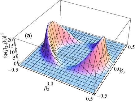
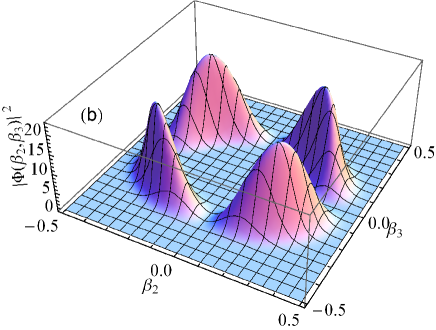
Figure 8: (Color online) Density distribution $\rho_{nkI}(\beta_{2},\beta_{3})=|\Phi^{\pi}_{nkI}(\beta_{2},\beta_{3})|^{2}$ for: (a) $k=1$, $I=2$ and (b) $k=2$, $I=1$ at $n=0$ with schematic parameters (see the text). The model space corresponds to the $\beta_{2}>0$ half-plane.

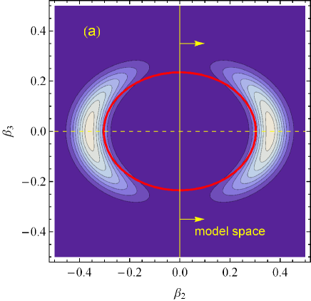
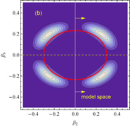
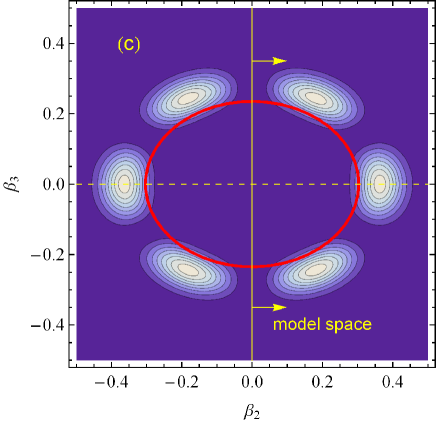
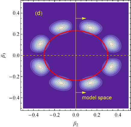
Figure 9: (Color online) Contour plots of the density distribution $\rho_{nkI}(\beta_{2},\beta_{3})$ for: (a) $k=1$, $I=2$, (b) $k=2$, $I=1$, (c) $k=3$, $I=2$ and (d) $k=4$, $I=1$ at $n=0$ with the schematic parameters (see the text). The ellipsoidal curves outline the potential bottom. The model space corresponds to the $\beta_{2}>0$ half-plane.

The density distribution of the CQOM vibration state in the space of the quadrupole-octupole shapes is given by the square of the wave function (17), $\rho_{nkI}(\beta_{2},\beta_{3})=|\Phi^{\pi}_{nkI}(\beta_{2},\beta_{3})|^{2}$, after a transformation from the ellipsoidal coordinates $(\eta,\phi)$ to the deformation coordinates $(\beta_{2},\beta_{3})$. In Fig. 8 three-dimensional plots of $\rho_{nkI}$ are given for the lowest $k=1$ and $k=2$ states for $n=0$ and for the schematic parameter values $\omega=0.3\,$MeV/$\hbar$, $b=3\,\hbar^{-2}$, $d_{0}=100\,\hbar^{2}$, $d_{2}=300\,\hbar^{2}$/MeV, $d_{3}=500\,\hbar^{2}$/MeV. Note that according to the discussion in the end of Sec. 3 the shape of the potential is determined unambiguously when the values of the inertia parameters $d_{2}$ and $d_{3}$ are given. In Fig. 9 two-dimensional plots showing the maxima of $\rho_{nkI}$ for $k=1-4$ are given together with contours showing the ellipsoidal potential bottom for the above set of schematic parameters.

Appendix B: Explicit form of the integrals over $\eta$

The integrals over $\eta$, (39) and (40), can be written in the following common form after taking into account the explicit expression for the radial wave functions (13)

$$S_{l}(n_{i},I_{i};n_{f},I_{f}) = \int_{0}^{\infty}d\eta\psi_{n_{f}}^{I_{f}}(\eta)\eta^{l+1}\psi_{n_{i}}^{I_{i}}(\eta)$$ (48)

$$= N\int_{0}^{\infty}e^{-c\eta^{2}}c^{s_{f}}\eta^{2s_{f}}L_{n_{f}}^{2s_{f}}(c\eta^{2})\eta^{l+1}c^{s_{i}}\eta^{2s_{i}}L_{n_{i}}^{2s_{i}}(c\eta^{2})d\eta,$$

where $l=1,2$, $s_{i}=(1/2)\sqrt{k_{i}^{2}+bX(I_{i})}$,  $s_{f}=(1/2)\sqrt{k_{f}^{2}+bX(I_{f})}$ and

$$N=N_{n_{i},n_{f}}(c,s_{i},s_{f})=2c\left[\frac{\Gamma(n_{f}+1)\Gamma(n_{i}+1)}{\Gamma(n_{f}+2s_{f}+1)\Gamma(n_{i}+2s_{i}+1)}\right]^{\frac{1}{2}}.$$ (49)

To derive an explicit expression for the integral (48) one can apply the substitution $c\eta^{2}=x$ with $dx=2c\eta d\eta$, such that

$$\eta^{l+1}d\eta=\frac{1}{2c^{1+l/2}}x^{l/2}dx.$$ (50)

Then Eq. (48) reads as

$$S_{l}(n_{i},I_{i};n_{f},I_{f})=\frac{N_{n_{i},n_{f}}(c,s_{i},s_{f})}{2c^{1+l/2}}\int_{0}^{\infty}e^{-x}x^{s_{i}+s_{f}+\frac{l}{2}}L_{n_{f}}^{2s_{f}}(x)L_{n_{i}}^{2s_{i}}(x)dx.$$ (51)

By using known formulas for integration of two generalized Laguerre polynomials with different real ranks [37], [38] one obtains (51) in the following explicit form

$$S_{l}(n_{i},I_{i};n_{f},I_{f})$$

$$= \frac{N_{n_{i},n_{f}}(c,s_{i},s_{f})}{2c^{1+l/2}}\frac{\Gamma(n_{f}+2s_{f}+1)}{\Gamma(1+2s_{f})}\frac{\Gamma(n_{i}+s_{i}-s_{f}-\frac{l}{2})}{\Gamma(s_{i}-s_{f}-1)}\frac{\Gamma(s_{i}+s_{f}+\frac{l}{2}+1)}{n_{i}!n_{f}!}$$

$$\times {}_{3}F_{2}\left(-n_{f},s_{i}+s_{f}+\frac{l}{2}+1,s_{f}-s_{i}+\frac{l}{2}+1;2s_{f}+1,s_{f}-s_{i}+\frac{l}{2}+1-n_{i};1\right),$$

where ${}_{3}F_{2}$ denotes a generalized hypergeometric function [39]. The generalized hypergeometric function ${}_{3}F_{2}$ is calculated numerically through a summation of its series representation for which a Fortran code is available [40]. It can be easily checked that if the first argument of ${}_{3}F_{2}$ in (Appendix B: Explicit form of the integrals over $\eta$) is zero, $n_{f}=0$, one has ${}_{3}F_{2}=1$. In this case Eq. (Appendix B: Explicit form of the integrals over $\eta$) reduces to the following simpler expression

$$S_{l}(n_{i},I_{i};0,I_{f}) = \frac{1}{c^{\,l/2}}\frac{\Gamma(s_{i}+s_{f}+\frac{l}{2}+1)\Gamma(n_{i}+s_{i}-s_{f}-\frac{l}{2})}{\sqrt{n_{i}!\Gamma(2s_{f}+1)\Gamma(n_{i}+2s_{i}+1)}\Gamma(s_{i}-s_{f}-\frac{l}{2})}.$$ (53)

This corresponds to a transition from a non-yrast to an yrast state. The integrals for the yrast intraband transitions, Eqs. (50) and (51) in [18], are directly obtained from Eq. (53) when $n_{i}=0$. Simple explicit forms of the $S_{l}$ integrals for interband and intraband transitions in the particular cases up to $n=2$, which are of practical interest, are given below

$$S_{l}(1,I_{i};1,I_{f})$$ (54)

$$= \frac{1}{c^{\,l/2}}\Bigl{[}(2s_{i}+1)(2s_{f}+1)-(s_{i}+s_{f}-\frac{l}{2})(s_{i}+s_{f}+\frac{l}{2}+1)\Bigr{]}$$

$$\times \frac{\Gamma(s_{i}+s_{f}+\frac{l}{2}+1)}{\sqrt{\Gamma(2s_{i}+2)\Gamma(2s_{f}+2)}},$$

$$S_{l}(2,I_{i};1,I_{f})$$ (55)

$$= \frac{\sqrt{2}}{2c^{\,l/2}}\biggl{\{}2(s_{i}+1)(2s_{i}+1)(2s_{f}+1)-(s_{i}+s_{f}+\frac{l}{2}+1)\biggr{.}$$

$$\times \biggl{.}\Bigl{[}2(s_{i}+1)(2s_{i}+4s_{f}+3)-(s_{i}+s_{f}+\frac{l}{2}+2)(3s_{i}+s_{f}-\frac{l}{2}+2)\Bigr{]}\biggr{\}}$$

$$\times \frac{\Gamma(s_{i}+s_{f}+\frac{l}{2}+1)}{\sqrt{\Gamma(2s_{i}+3)\Gamma(2s_{f}+2)}}.$$

$$S_{l}(2,I_{i};2,I_{f})$$ (56)

$$= \frac{1}{2c^{\,l/2}}\Biggl{\{}4(s_{i}+1)(2s_{i}+1)(s_{f}+1)(2s_{f}+1)\Biggr{.}$$

$$- (s_{i}+s_{f}+\frac{l}{2}+1)\biggl{[}16(s_{i}+1)(s_{f}+1)(s_{i}+s_{f}+1)\biggr{.}$$

$$- (s_{i}+s_{f}+\frac{l}{2}+2)\Bigl{\{}2(s_{i}+1)(2s_{i}+1)+2(s_{f}+1)(2s_{f}+1)+16(s_{i}+1)(s_{f}+1)\Bigr{.}$$

$$- \Biggl{.}\biggl{.}\Bigl{.}(s_{i}+s_{f}+\frac{l}{2}+3)(3s_{i}+3s_{f}-\frac{l}{2}+4)\Bigr{\}}\biggr{]}\Biggr{\}}\frac{\Gamma(s_{i}+s_{f}+\frac{l}{2}+1)}{\sqrt{\Gamma(2s_{i}+3)\Gamma(2s_{f}+3)}}.$$

Appendix C: Explicit form of the integrals over $\phi$

The integrals over the angular variable $\phi$, (41), with the relevant parities $\pi_{i}$ and $\pi_{f}$ can be obtained in the following explicit forms. For $\lambda=2$ the integral $I_{2}^{\pm\pm}$ with $k_{1}=k_{2}=k=\mbox{odd}$ (++) or even $(--)$ is

$$I_{2}^{\pm\pm}(k)=\frac{2}{\pi}\mbox{Cat}+\frac{(-1)^{k+1}}{4k}\left[1+\frac{4}{\pi}\sum_{m=1}^{2k-1}\frac{\sin(m\pi/2)}{m}\right],$$ (57)

where $\mbox{Cat}=\sum_{n=0}^{\infty}\frac{(-1)^{n}}{(2n+1)^{2}}\approx 0.915965594177...$ is the Catalan constant. In the case of $k_{1}\neq k_{2}$, both odd or even, the integral is

$$I_{2}^{\pm\pm}(k_{1},k_{2}) = \frac{1}{2|k_{2}-k_{1}|}\left[1+\frac{4}{\pi}\sum_{m=1}^{|k_{2}-k_{1}|-1}\frac{\sin(m\pi/2)}{m}\right]$$

$$+ \frac{(-1)^{k_{1}+1}}{2(k_{2}+k_{1})}\left[1+\frac{4}{\pi}\sum_{m=1}^{k_{2}+k_{1}-1}\frac{\sin(m\pi/2)}{m}\right].$$

For $\lambda=3$ one has

$$I_{3}^{+-}(k_{1},k_{2})=\frac{2k_{2}}{k_{2}^{2}-k_{1}^{2}}-\frac{1}{\pi}\left[\frac{(-1)^{(k_{2}-k_{1}-1)/2}}{(k_{2}-k_{1})^{2}}+\frac{(-1)^{(k_{2}+k_{1}-1)/2}}{(k_{2}+k_{1})^{2}}\right],$$ (59)

where $k_{1}=1,3,5,\dots\ ,\ \ k_{2}=2,4,6,\dots$ For $\lambda=1$ the integral is obtained in the form of an infinite, but reasonably converging series

$$I_{1}^{+-} = \frac{1}{2\pi}\sum_{m=\pm 1}^{\pm\infty}\sum_{n=\pm 1}^{\pm\infty}\sum_{\nu=\pm 1}\frac{\mbox{sign}(-n)}{|mn|}$$ (60)

$$\times \left[(1-\delta_{k_{2}+\nu k_{1},-m-n})\frac{\sin[(k_{2}+\nu k_{1}+m+n)\frac{\pi}{2}]}{(k_{2}+\nu k_{1}+m+n)}+\frac{\pi}{2}\delta_{k_{2}+\nu k_{1},-m-n}\right],$$

where $k_{1}=1,3,5,\dots\ ,\ \ k_{2}=2,4,6,\dots$

Table 1: Parameters of the model fits.

Nucl	$\omega$ [MeV/$\hbar$]	$b$ [$\hbar^{-2}$]	$d_{0}$ [$\hbar^{2}$]	$c$	$p$	$e^{1}_{eff}$ [e]
152Sm	0.295	2.450	78.8	113.2	0.854	1.01
154Sm	0.205	4.625	108.5	132.6	0.808	1.017
154Gd	0.306	2.948	114.7	113.4	0.777	1.048
156Gd	0.439	1.642	197.6	141.5	0.849	0.723
158Gd	0.168	3.626	42.6	39.7	0.864	0.435
236U	0.402	1.404	539.3	343.4	0.949	0.134
100Mo	0.318	2.674	1.366	54.6	0.715	0.282

Table 2: Resulting mass parameters $B_{2}$ and $B_{3}$ (in $\hbar^{2}/$MeV), Eq. (3), and parameters of the model potential $C_{2}$ and $C_{3}$ (in MeV), $d_{2}$ and $d_{3}$ (in $\hbar^{2}/$MeV), Eq. (4). The semi-axes (sa) of the ellipsoidal potential bottom $\beta_{2}^{\mbox{\scriptsize sa}}$ and $\beta_{3}^{\mbox{\scriptsize sa}}$, Eq. (46), at angular momentum $I=0$ are given in columns 8 and 9.

Nucl	$B_{2}$	$B_{3}$	$C_{2}$	$C_{3}$	$d_{2}$	$d_{3}$	$\beta_{2}^{\mbox{\scriptsize sa}}$	$\beta_{3}^{\mbox{\scriptsize sa}}$
152Sm	525	241	45.8	21.0	429	197	0.252	0.371
154Sm	987	303	41.7	12.8	427	131	0.279	0.504
154Gd	613	127	57.6	11.9	416	86	0.263	0.578
156Gd	447	197	86.2	38.0	545	240	0.255	0.384
158Gd	317	156	8.9	4.4	175	86	0.407	0.579
236U	948	760	153	123	1351	1083	0.226	0.252
100Mo	337	7	34.0	0.7	252	6	0.112	0.759

Table 3: Theoretical and experimental values of B(E1), B(E2) and B(E3) transition probabilities in Weisskopf units (W.u.) for alternating-parity spectra of several even-even nuclei. Notations: $g$ (ground-state band), $b1$ (first $\beta$-band), $b2$ (second $\beta$-band), $n1$ (first negative-parity band), $n2$ (second negative-parity band), $n3$ (third negative-parity band). The data are taken from [35] except for those for B$(E3;3_{n1}^{-}\rightarrow 0_{g}^{+})$ transitions, which are taken from [36]. The parity signs $(+)$ for the even and $(-)$ for the odd angular momenta, respectively are omitted in the labels of the states to avoid overloading of notations. The uncertainties (in parentheses) refer to the last significant digits in the experimental data.

Mult	Transition	Th [W.u.]	Exp [W.u.]	Mult	Transition	Th [W.u.]	Exp [W.u.]
152Sm
$E2$	$2_{g}$ $\rightarrow$ $0_{g}$	141	144 (3)	$E2$	$3_{n2}$ $\rightarrow$ $1_{n2}$	52
$E2$	$4_{g}$ $\rightarrow$ $2_{g}$	210	209 (3)	$E2$	$5_{n2}$ $\rightarrow$ $3_{n2}$	63
$E2$	$6_{g}$ $\rightarrow$ $4_{g}$	248	245 (5)	$E3$	$3_{n1}$ $\rightarrow$ $0_{g}$	14	14 (2)
$E2$	$8_{g}$ $\rightarrow$ $6_{g}$	284	285 (14)	$E3$	$3_{n2}$ $\rightarrow$ $0_{b1}$	10
$E2$	$10_{g}$ $\rightarrow$ $8_{g}$	322	320 (3)	$E3$	$1_{n1}$ $\rightarrow$ $4_{g}$	69
$E2$	$12_{g}$ $\rightarrow$ $10_{g}$	363		$E3$	$1_{n2}$ $\rightarrow$ $4_{b1}$	70
$E1$	$1_{n1}$ $\rightarrow$ $0_{g}$	0.0041	0.0042 (4)	$E2$	$2_{b1}$ $\rightarrow$ $0_{g}$	1.26	0.92 (8)
$E1$	$1_{n1}$ $\rightarrow$ $2_{g}$	0.0088	0.0077 (7)	$E2$	$4_{b1}$ $\rightarrow$ $2_{g}$	0.2	0.7 (2)
$E1$	$3_{n1}$ $\rightarrow$ $2_{g}$	0.0056	0.0081 (16)	$E2$	$2_{b1}$ $\rightarrow$ $2_{g}$	4.6	5.5 (5)
$E1$	$3_{n1}$ $\rightarrow$ $4_{g}$	0.0087	0.0082 (16)	$E2$	$4_{b1}$ $\rightarrow$ $4_{g}$	4.2	5.4 (13)
$E1$	$1_{n2}$ $\rightarrow$ $0_{b1}$	0.0041		$E2$	$2_{b1}$ $\rightarrow$ $4_{g}$	27.4	19.2 (18)
$E1$	$1_{n2}$ $\rightarrow$ $2_{b1}$	0.0095		$E2$	$4_{b1}$ $\rightarrow$ $6_{g}$	35	4 (2)
$E2$	$2_{b1}$ $\rightarrow$ $0_{b1}$	160	107 (27)	$E2$	$0_{b1}$ $\rightarrow$ $2_{g}$	30
$E2$	$4_{b1}$ $\rightarrow$ $2_{b1}$	232	204 (38)	$E1$	$1_{n1}$ $\rightarrow$ $2_{b1}$	0.00402	0.00013 (4)
$E2$	$3_{n1}$ $\rightarrow$ $1_{n1}$	47		$E1$	$1_{n1}$ $\rightarrow$ $0_{b1}$	0.0023
$E2$	$5_{n1}$ $\rightarrow$ $3_{n1}$	58		$E1$	$1_{n2}$ $\rightarrow$ $0_{g}$	0.00006
154Sm
$E2$	$2_{g}$ $\rightarrow$ $0_{g}$	168	176 (1)	$E2$	$5_{n2}$ $\rightarrow$ $3_{n2}$	82
$E2$	$4_{g}$ $\rightarrow$ $2_{g}$	247	245 (6)	$E2$	$3_{n3}$ $\rightarrow$ $1_{n3}$	72
$E2$	$6_{g}$ $\rightarrow$ $4_{g}$	287	289 (8)	$E3$	$3_{n1}$ $\rightarrow$ $0_{g}$	10	10 (2)
$E2$	$8_{g}$ $\rightarrow$ $6_{g}$	322	319 (17)	$E3$	$1_{n1}$ $\rightarrow$ $4_{g}$	50
$E2$	$10_{g}$ $\rightarrow$ $8_{g}$	358	314 (16)	$E3$	$3_{n2}$ $\rightarrow$ $0_{b1}$	77
$E2$	$12_{g}$ $\rightarrow$ $10_{g}$	398	282 (19)	$E3$	$1_{n2}$ $\rightarrow$ $4_{b1}$	381
$E1$	$1_{n1}$ $\rightarrow$ $0_{g}$	0.0051	0.0058 (4)	$E3$	$3_{n3}$ $\rightarrow$ $0_{b2}$	6
$E1$	$1_{n1}$ $\rightarrow$ $2_{g}$	0.0110	0.0113 (7)	$E3$	$1_{n3}$ $\rightarrow$ $4_{b2}$	62
$E1$	$3_{n1}$ $\rightarrow$ $2_{g}$	0.0069	0.0080 (11)	$E2$	$0_{b1}$ $\rightarrow$ $2_{g}$	1	12 (3)
$E1$	$3_{n1}$ $\rightarrow$ $4_{g}$	0.0106	0.0092 (13)	$E2$	$2_{b1}$ $\rightarrow$ $0_{g}$	0.36	$<$0.58
$E1$	$1_{n2}$ $\rightarrow$ $0_{b1}$	0.0109		$E2$	$2_{b1}$ $\rightarrow$ $2_{g}$	0.39	$<$1.3
$E1$	$1_{n2}$ $\rightarrow$ $2_{b1}$	0.0231		$E2$	$2_{b1}$ $\rightarrow$ $4_{g}$	0.27	$<$2.4
$E1$	$1_{n3}$ $\rightarrow$ $0_{b2}$	0.0044		$E2$	$0_{b2}$ $\rightarrow$ $2_{g}$	$5\times 10^{-6}$
$E1$	$1_{n3}$ $\rightarrow$ $2_{b2}$	0.0109		$E2$	$0_{b2}$ $\rightarrow$ $2_{b1}$	16
$E2$	$2_{b1}$ $\rightarrow$ $0_{b1}$	65		$E1$	$0_{b1}$ $\rightarrow$ $1_{n1}$	0.0005
$E2$	$4_{b1}$ $\rightarrow$ $2_{b1}$	93		$E1$	$1_{n2}$ $\rightarrow$ $0_{g}$	0.0005
$E2$	$2_{b2}$ $\rightarrow$ $0_{b2}$	68		$E1$	$1_{n2}$ $\rightarrow$ $0_{b2}$	0.0058
$E2$	$4_{b2}$ $\rightarrow$ $2_{b2}$	97		$E1$	$1_{n3}$ $\rightarrow$ $0_{b1}$	$3\times 10^{-7}$
$E2$	$3_{n1}$ $\rightarrow$ $1_{n1}$	60		$E1$	$1_{n3}$ $\rightarrow$ $0_{g}$	$8\times 10^{-5}$
$E2$	$5_{n1}$ $\rightarrow$ $3_{n1}$	72		$E3$	$3_{n2}$ $\rightarrow$ $0_{g}$	1.7
$E2$	$3_{n2}$ $\rightarrow$ $1_{n2}$	69		$E3$	$3_{n3}$ $\rightarrow$ $0_{g}$	0.4
154Gd
$E2$	$2_{g}$ $\rightarrow$ $0_{g}$	160	157 (1)	$E2$	$5_{n2}$ $\rightarrow$ $3_{n2}$	64
$E2$	$4_{g}$ $\rightarrow$ $2_{g}$	235	245 (9)	$E2$	$3_{n3}$ $\rightarrow$ $1_{n3}$	51
$E2$	$6_{g}$ $\rightarrow$ $4_{g}$	273	285 (15)	$E3$	$3_{n1}$ $\rightarrow$ $0_{g}$	21	21 (5)
$E2$	$8_{g}$ $\rightarrow$ $6_{g}$	306	312 (17)	$E3$	$3_{n2}$ $\rightarrow$ $0_{b1}$	32
$E2$	$10_{g}$ $\rightarrow$ $8_{g}$	340	360 (4)	$E3$	$3_{n3}$ $\rightarrow$ $0_{b2}$	144
$E2$	$12_{g}$ $\rightarrow$ $10_{g}$	377		$E3$	$1_{n1}$ $\rightarrow$ $4_{g}$	102
$E1$	$1_{n1}$ $\rightarrow$ $0_{g}$	0.0102	0.0436	$E3$	$1_{n2}$ $\rightarrow$ $4_{b1}$	179
$E1$	$1_{n1}$ $\rightarrow$ $2_{g}$	0.0216	0.0485	$E3$	$1_{n3}$ $\rightarrow$ $4_{b2}$	708
$E1$	$3_{n1}$ $\rightarrow$ $2_{g}$	0.0137		$E2$	$0_{b1}$ $\rightarrow$ $2_{g}$	25	52 (8)
$E1$	$3_{n1}$ $\rightarrow$ $4_{g}$	0.0207		$E2$	$2_{b1}$ $\rightarrow$ $0_{g}$	1.23	0.86 (7)
$E1$	$1_{n2}$ $\rightarrow$ $0_{b1}$	0.0152		$E2$	$2_{b1}$ $\rightarrow$ $4_{g}$	22.6	19.6 (16)
$E1$	$1_{n2}$ $\rightarrow$ $2_{b1}$	0.0333		$E2$	$0_{b2}$ $\rightarrow$ $2_{g}$	0.0553
$E1$	$1_{n3}$ $\rightarrow$ $0_{b2}$	0.0333		$E2$	$0_{b2}$ $\rightarrow$ $2_{b1}$	14
$E1$	$1_{n3}$ $\rightarrow$ $2_{b2}$	0.0706		$E1$	$1_{n1}$ $\rightarrow$ $0_{b1}$	0.0054	0.0057
$E2$	$2_{b1}$ $\rightarrow$ $0_{b1}$	177	97 (10)	$E1$	$1_{n1}$ $\rightarrow$ $2_{b1}$	0.0099	0.0064
$E2$	$4_{b1}$ $\rightarrow$ $2_{b1}$	256		$E1$	$1_{n2}$ $\rightarrow$ $0_{g}$	2$\times 10^{-5}$
$E2$	$2_{b2}$ $\rightarrow$ $0_{b2}$	85		$E1$	$1_{n2}$ $\rightarrow$ $0_{b2}$	0.0094
$E2$	$4_{b2}$ $\rightarrow$ $2_{b2}$	122		$E1$	$1_{n3}$ $\rightarrow$ $0_{b1}$	0.00023
$E2$	$3_{n1}$ $\rightarrow$ $1_{n1}$	55		$E1$	$1_{n3}$ $\rightarrow$ $0_{g}$	2$\times 10^{-6}$
$E2$	$5_{n1}$ $\rightarrow$ $3_{n1}$	67		$E3$	$3_{n2}$ $\rightarrow$ $0_{g}$	1.8
$E2$	$3_{n2}$ $\rightarrow$ $1_{n2}$	54		$E3$	$3_{n3}$ $\rightarrow$ $0_{g}$	0.05
156Gd
$E2$	$2_{g}$ $\rightarrow$ $0_{g}$	150	187 (5)	$E2$	$3_{n2}$ $\rightarrow$ $1_{n2}$	44
$E2$	$4_{g}$ $\rightarrow$ $2_{g}$	219	263 (5)	$E2$	$5_{n2}$ $\rightarrow$ $3_{n2}$	53
$E2$	$6_{g}$ $\rightarrow$ $4_{g}$	249	295 (8)	$E3$	$3_{n1}$ $\rightarrow$ $0_{g}$	16.9	16.9 (7)
$E2$	$8_{g}$ $\rightarrow$ $6_{g}$	273	320 (14)	$E3$	$3_{n2}$ $\rightarrow$ $0_{b1}$	64
$E2$	$10_{g}$ $\rightarrow$ $8_{g}$	296	314 (14)	$E3$	$1_{n1}$ $\rightarrow$ $4_{g}$	73
$E2$	$12_{g}$ $\rightarrow$ $10_{g}$	321	300 (3)	$E3$	$1_{n2}$ $\rightarrow$ $4_{b1}$	282
$E1$	$1_{n1}$ $\rightarrow$ $0_{g}$	0.0006	0.0019 (14)	$E2$	$0_{b1}$ $\rightarrow$ $2_{g}$	5	8 (4)
$E1$	$1_{n1}$ $\rightarrow$ $2_{g}$	0.0013	0.0025 (18)	$E2$	$2_{b1}$ $\rightarrow$ $0_{g}$	0.32	0.63 (6)
$E1$	$3_{n1}$ $\rightarrow$ $2_{g}$	0.00083	0.00098 (21)	$E2$	$4_{b1}$ $\rightarrow$ $2_{g}$	0.1	1.3 (7)
$E1$	$3_{n1}$ $\rightarrow$ $4_{g}$	0.0012	0.00077 (16)	$E2$	$4_{b1}$ $\rightarrow$ $6_{g}$	5.6	2.1 (11)
$E1$	$1_{n2}$ $\rightarrow$ $0_{b1}$	0.0013		$E2$	$2_{b1}$ $\rightarrow$ $4_{g}$	4.3	4.1 (4)
$E1$	$1_{n2}$ $\rightarrow$ $2_{b1}$	0.0026	0.0005 (3)	$E1$	$1_{n1}$ $\rightarrow$ $0_{b1}$	0.0002	0.0004 (3)
$E1$	$3_{n2}$ $\rightarrow$ $2_{b1}$	0.0016		$E1$	$1_{n2}$ $\rightarrow$ $0_{g}$	$6\times 10^{-6}$	0.0019 (7)
$E2$	$2_{b1}$ $\rightarrow$ $0_{b1}$	74	52 (23)	$E1$	$1_{n2}$ $\rightarrow$ $2_{g}$	$2\times 10^{-5}$	0.0043 (15)
$E2$	$4_{b1}$ $\rightarrow$ $2_{b1}$	107	280 (15)	$E1$	$3_{n2}$ $\rightarrow$ $2_{g}$	$5\times 10^{-6}$	0.0019 (14)
$E2$	$6_{b1}$ $\rightarrow$ $4_{b1}$	120		$E1$	$3_{n2}$ $\rightarrow$ $4_{g}$	$2\times 10^{-5}$	0.0031 (4)
$E2$	$3_{n1}$ $\rightarrow$ $1_{n1}$	46		$E3$	$3_{n2}$ $\rightarrow$ $0_{g}$	0.21
$E2$	$5_{n1}$ $\rightarrow$ $3_{n1}$	56
158Gd
$E2$	$2_{g}$ $\rightarrow$ $0_{g}$	181	198 (6)	$E2$	$0_{b1}$ $\rightarrow$ $2_{g}$	8.7619	1.1652
$E2$	$4_{g}$ $\rightarrow$ $2_{g}$	274	289 (5)	$E2$	$2_{b1}$ $\rightarrow$ $0_{g}$	2.36	0.31 (4)
$E2$	$6_{g}$ $\rightarrow$ $4_{g}$	332		$E2$	$2_{b1}$ $\rightarrow$ $2_{g}$	2.913	0.079 (14)
$E2$	$8_{g}$ $\rightarrow$ $6_{g}$	393	330 (3)	$E2$	$4_{b1}$ $\rightarrow$ $4_{g}$	2.40	0.37
$E2$	$10_{g}$ $\rightarrow$ $8_{g}$	460	340 (3)	$E2$	$2_{b1}$ $\rightarrow$ $4_{g}$	2.96	1.39 (15)
$E2$	$12_{g}$ $\rightarrow$ $10_{g}$	532	310 (3)	$E2$	$0_{b2}$ $\rightarrow$ $2_{g}$	1.86	2.09
$E1$	$1_{n1}$ $\rightarrow$ $0_{g}$	0.0001	9.8443$\times 10^{-5}$(4)	$E2$	$2_{b2}$ $\rightarrow$ $0_{g}$	0.68	0.37 (4)
$E1$	$1_{n1}$ $\rightarrow$ $2_{g}$	2.5$\times 10^{-4}$	9.6515$\times 10^{-5}(6)$	$E2$	$2_{b2}$ $\rightarrow$ $4_{g}$	0.43	0.38 (6)
$E1$	$3_{n1}$ $\rightarrow$ $2_{g}$	0.00015	0.00033 (10)	$E2$	$4_{b1}$ $\rightarrow$ $2_{g}$	3.75	1.32
$E1$	$3_{n1}$ $\rightarrow$ $4_{g}$	0.00028	0.00029 (8)	$E2$	$4_{b1}$ $\rightarrow$ $6_{g}$	1.30	3.16
$E1$	$5_{n1}$ $\rightarrow$ $4_{g}$	2.02$\times 10^{-4}$	7.4324$\times 10^{-4}$(13)	$E2$	$0_{b2}$ $\rightarrow$ $2_{b1}$	57
$E1$	$5_{n1}$ $\rightarrow$ $6_{g}$	3.62$\times 10^{-4}$	5.8691$\times 10^{-4}$(8)	$E1$	$0_{b1}$ $\rightarrow$ $1_{n1}$	2.7$\times 10^{-5}$	3.314$\times 10^{-6}$
$E1$	$3_{n2}$ $\rightarrow$ $2_{b1}$	0.00011	$>$ 0.00035	$E1$	$2_{b1}$ $\rightarrow$ $1_{n1}$	8.3$\times 10^{-6}$	6.4$\times 10^{-5}$(8)
$E1$	$1_{n2}$ $\rightarrow$ $0_{b1}$	8.02$\times 10^{-5}$		$E1$	$2_{b1}$ $\rightarrow$ $3_{n1}$	2$\times 10^{-5}$	1.89$\times 10^{-4}$(24)
$E1$	$1_{n2}$ $\rightarrow$ $2_{b1}$	0.0002		$E1$	$1_{n2}$ $\rightarrow$ $2_{g}$	4$\times 10^{-5}$	0.0064
$E1$	$1_{n3}$ $\rightarrow$ $0_{b2}$	0.0004		$E1$	$1_{n2}$ $\rightarrow$ $0_{g}$	2$\times 10^{-5}$	0.0035 (12)
$E1$	$1_{n3}$ $\rightarrow$ $2_{b2}$	0.0009		$E1$	$3_{n2}$ $\rightarrow$ $2_{g}$	3$\times 10^{-5}$	$>$0.0011
$E1$	$3_{n3}$ $\rightarrow$ $2_{b2}$	0.0005		$E1$	$3_{n2}$ $\rightarrow$ $4_{g}$	3$\times 10^{-5}$	$>$0.0015
$E2$	$2_{b1}$ $\rightarrow$ $0_{b1}$	200		$E1$	$0_{b2}$ $\rightarrow$ $1_{n1}$	2$\times 10^{-7}$	5.7831$\times 10^{-5}$
$E2$	$4_{b1}$ $\rightarrow$ $2_{b1}$	288	455	$E1$	$2_{b2}$ $\rightarrow$ $1_{n1}$	2$\times 10^{-8}$	2.7$\times 10^{-6}$(19)
$E2$	$2_{b2}$ $\rightarrow$ $0_{b2}$	217		$E1$	$2_{b2}$ $\rightarrow$ $3_{n1}$	2$\times 10^{-7}$	3.7$\times 10^{-5}$(5)
$E2$	$4_{b2}$ $\rightarrow$ $2_{b2}$	308		$E1$	$0_{b2}$ $\rightarrow$ $1_{n2}$	6$\times 10^{-5}$	6.02$\times 10^{-4}$
$E2$	$3_{n1}$ $\rightarrow$ $1_{n1}$	185		$E1$	$2_{b2}$ $\rightarrow$ $1_{n2}$	1.8$\times 10^{-5}$	1.50$\times 10^{-4}$(21)
$E2$	$5_{n1}$ $\rightarrow$ $3_{n1}$	227	369 (6)	$E1$	$2_{b2}$ $\rightarrow$ $3_{n2}$	4.2$\times 10^{-5}$	2.40$\times 10^{-4}$(5)
$E2$	$3_{n2}$ $\rightarrow$ $1_{n2}$	200	$>$ 1600	$E1$	$4_{b1}$ $\rightarrow$ $3_{n1}$	7.7$\times 10^{-6}$	4.63$\times 10^{-4}$
$E2$	$5_{n2}$ $\rightarrow$ $3_{n2}$	240		$E1$	$4_{b1}$ $\rightarrow$ $5_{n1}$	2.1$\times 10^{-5}$	6.12$\times 10^{-4}$
$E2$	$3_{n3}$ $\rightarrow$ $1_{n3}$	241		$E1$	$1_{n2}$ $\rightarrow$ $0_{b2}$	2$\times 10^{-5}$
$E3$	$3_{n1}$ $\rightarrow$ $0_{g}$	11.9	11.9 (7)	$E1$	$1_{n3}$ $\rightarrow$ $0_{b1}$	3$\times 10^{-6}$
$E3$	$1_{n1}$ $\rightarrow$ $4_{g}$	81		$E1$	$1_{n3}$ $\rightarrow$ $0_{g}$	0.00001
$E3$	$3_{n2}$ $\rightarrow$ $0_{b1}$	519		$E3$	$3_{n2}$ $\rightarrow$ $0_{g}$	5
$E3$	$3_{n3}$ $\rightarrow$ $0_{b2}$	102		$E3$	$3_{n3}$ $\rightarrow$ $0_{g}$	2
236U
$E2$	$2_{g}$ $\rightarrow$ $0_{g}$	237	250 (10)	$E2$	$2_{b1}$ $\rightarrow$ $0_{b1}$	112
$E2$	$4_{g}$ $\rightarrow$ $2_{g}$	342	357 (23)	$E2$	$4_{b1}$ $\rightarrow$ $2_{b1}$	160
$E2$	$6_{g}$ $\rightarrow$ $4_{g}$	382	385 (22)	$E2$	$3_{n1}$ $\rightarrow$ $1_{n1}$	68
$E2$	$8_{g}$ $\rightarrow$ $6_{g}$	408	390 (4)	$E2$	$5_{n1}$ $\rightarrow$ $3_{n1}$	80
$E2$	$10_{g}$ $\rightarrow$ $8_{g}$	429	360 (4)	$E2$	$7_{n1}$ $\rightarrow$ $5_{n1}$	87
$E2$	$12_{g}$ $\rightarrow$ $10_{g}$	450	410 (7)	$E2$	$3_{n2}$ $\rightarrow$ $1_{n2}$	54
$E2$	$14_{g}$ $\rightarrow$ $12_{g}$	471	450 (5)	$E2$	$5_{n2}$ $\rightarrow$ $3_{n2}$	64
$E2$	$16_{g}$ $\rightarrow$ $14_{g}$	493	380 (4)	$E3$	$1_{n1}$ $\rightarrow$ $4_{g}$	62	62 (9)
$E2$	$18_{g}$ $\rightarrow$ $16_{g}$	516	490 (5)	$E3$	$3_{n1}$ $\rightarrow$ $0_{g}$	15	23 (3)
$E2$	$20_{g}$ $\rightarrow$ $18_{g}$	539	510 (8)	$E3$	$1_{n2}$ $\rightarrow$ $4_{b1}$	695
$E2$	$22_{g}$ $\rightarrow$ $20_{g}$	564	520 (12)	$E3$	$3_{n2}$ $\rightarrow$ $0_{b1}$	172
$E2$	$24_{g}$ $\rightarrow$ $22_{g}$	590	670 (13)	$E2$	$0_{b1}$ $\rightarrow$ $2_{g}$	6
$E2$	$26_{g}$ $\rightarrow$ $24_{g}$	617	670 (19)	$E2$	$2_{b1}$ $\rightarrow$ $0_{g}$	0.66
$E2$	$28_{g}$ $\rightarrow$ $26_{g}$	645	1100 (5)	$E2$	$4_{b1}$ $\rightarrow$ $2_{g}$	0.59
$E1$	$1_{n1}$ $\rightarrow$ $0_{g}$	2.7$\times 10^{-8}$	2.7$\times 10^{-8}$(4)	$E2$	$2_{b1}$ $\rightarrow$ $4_{g}$	4
$E1$	$1_{n1}$ $\rightarrow$ $2_{g}$	5.5$\times 10^{-8}$		$E1$	$0_{b1}$ $\rightarrow$ $1_{n1}$	1.2$\times 10^{-8}$
$E1$	$3_{n1}$ $\rightarrow$ $2_{g}$	3.5$\times 10^{-8}$		$E1$	$2_{b1}$ $\rightarrow$ $1_{n1}$	4.6$\times 10^{-9}$
$E1$	$3_{n1}$ $\rightarrow$ $4_{g}$	4.8$\times 10^{-8}$		$E1$	$1_{n2}$ $\rightarrow$ $0_{g}$	1.6$\times 10^{-9}$
$E1$	$1_{n2}$ $\rightarrow$ $0_{b1}$	2.0$\times 10^{-8}$		$E3$	$3_{b2}$ $\rightarrow$ $0_{g}$	0.14
$E1$	$1_{n2}$ $\rightarrow$ $2_{b1}$	4.0$\times 10^{-8}$
100Mo
$E2$	$2_{g}$ $\rightarrow$ $0_{g}$	22.7	37.0 (7)	$E2$	$3_{n1}$ $\rightarrow$ $1_{n1}$	16
$E2$	$4_{g}$ $\rightarrow$ $2_{g}$	50	69 (4)	$E2$	$5_{n1}$ $\rightarrow$ $3_{n1}$	21
$E2$	$6_{g}$ $\rightarrow$ $4_{g}$	84	94 (14)	$E2$	$7_{n1}$ $\rightarrow$ $5_{n1}$	26
$E2$	$8_{g}$ $\rightarrow$ $6_{g}$	120	123 (18)	$E2$	$3_{n2}$ $\rightarrow$ $1_{n2}$	18
$E2$	$10_{g}$ $\rightarrow$ $8_{g}$	156		$E2$	$5_{n2}$ $\rightarrow$ $3_{n2}$	22
$E1$	$1_{n1}$ $\rightarrow$ $0_{g}$	2$\times 10^{-6}$		$E3$	$3_{n1}$ $\rightarrow$ $0_{g}$	34	34 (3)
$E1$	$1_{n1}$ $\rightarrow$ $2_{g}$	1$\times 10^{-5}$		$E3$	$3_{n2}$ $\rightarrow$ $0_{b1}$	5
$E1$	$3_{n1}$ $\rightarrow$ $2_{g}$	7$\times 10^{-6}$	2.7$\times 10^{-6}$(9)	$E3$	$1_{n1}$ $\rightarrow$ $4_{g}$	899
$E1$	$3_{n1}$ $\rightarrow$ $4_{g}$	2$\times 10^{-5}$		$E2$	$0_{b1}$ $\rightarrow$ $2_{g}$	72	92 (4)
$E1$	$1_{n2}$ $\rightarrow$ $0_{b1}$	2$\times 10^{-7}$		$E2$	$2_{b1}$ $\rightarrow$ $0_{g}$	0.5	0.62 (5)
$E1$	$1_{n2}$ $\rightarrow$ $2_{b1}$	1$\times 10^{-5}$		$E2$	$4_{b1}$ $\rightarrow$ $2_{g}$	3
$E1$	$3_{n2}$ $\rightarrow$ $2_{b1}$	3$\times 10^{-6}$		$E1$	$1_{n1}$ $\rightarrow$ $0_{b1}$	$8\times 10^{-6}$
$E1$	$3_{n2}$ $\rightarrow$ $4_{b1}$	3$\times 10^{-5}$		$E1$	$1_{n1}$ $\rightarrow$ $2_{b1}$	$2\times 10^{-5}$
$E2$	$2_{b1}$ $\rightarrow$ $0_{b1}$	25.4	5.5 (8)	$E1$	$3_{n1}$ $\rightarrow$ $2_{b1}$	1.4$\times 10^{-5}$	2.5$\times 10^{-5}$(8)
$E2$	$4_{b1}$ $\rightarrow$ $2_{b1}$	45		$E1$	$1_{n2}$ $\rightarrow$ $0_{g}$	5$\times 10^{-7}$
$E2$	$6_{b1}$ $\rightarrow$ $4_{b1}$	75		$E3$	$3_{n2}$ $\rightarrow$ $0_{g}$	22

References

- [1] P. A. Butler and W. Nazarewicz, Rev. Mod. Phys. 68, 349 (1996).
- [2] Y. A. Akovali, Nucl. Data Sheets 77, 433 (1996).
- [3] A. Artna-Cohen, Nucl. Data Sheets 80, 227 (1997).
- [4] J. F. C. Cocks et al, Phys. Rev. Lett. 78, 2920 (1997).
- [5] H. J. Krappe and U. Wille, Nucl. Phys. A 124, 641 (1969).
- [6] G. A. Leander, R. K. Sheline, P. Möller, P. Olanders, I. Ragnarsson, and A. J. Sierk, Nucl. Phys. A 388, 452 (1982).
- [7] R. V. Jolos, P. von Brentano, and F. Dönau, J. Phys. G: Nucl. Part. Phys. 19, L151 (1993).
- [8] R. V. Jolos, P. von Brentano, Phys. Rev. C 49, R2301 (1994).
- [9] A. Ya. Dzyublik and V. Yu. Denisov, Yad. Fiz. 56, 30 (1993) [Phys. At. Nucl. 56, 303 (1993)].
- [10] V. Yu. Denisov and A. Ya. Dzyublik, Nucl. Phys. A 589, 17 (1995).
- [11] N. V. Zamfir and D. Kusnezov, Phys. Rev. C 63, 054306 (2001).
- [12] T. M. Shneidman, G. G. Adamian, N. V. Antonenko, R. V. Jolos and W. Scheid, Phys. Rev. C 67, 014313 (2003).
- [13] D. Bonatsos, D. Lenis, N. Minkov, D. Petrellis, and P. Yotov, Phys. Rev. C 71, 064309 (2005).
- [14] A. A. Raduta and D. Ionescu, Phys. Rev. C 67, 044312 (2003).
- [15] A. A. Raduta, D. Ionescu, I. I. Ursu and A. Faessler, Nucl. Phys. A 720, 43 (2003).
- [16] A. A. Raduta, Al. H. Raduta, and C. M. Raduta, Phys. Rev. C 74, 044312 (2006).
- [17] N. Minkov, P. Yotov, S. Drenska and W. Scheid, J. Phys. G: Nucl. Part. Phys. 32, 497 (2006).
- [18] N. Minkov, P. Yotov, S. Drenska, W. Scheid, D. Bonatsos, D. Lenis and D. Petrellis, Phys. Rev. C 73, 044315 (2006).
- [19] P. G. Bizzeti and A. M. Bizzeti-Sona, Phys. Rev. C 77, 024320 (2008).
- [20] B. Buck, A. C. Merchant and S. M. Perez, J. Phys. G: Nucl. Part. Phys. 35, 085101 (2008).
- [21] A. Góźdź, A. Szulerecka, A. Dobrowolski and J. Dudek, Int. J. Mod. Phys E 20, 199 (2011).
- [22] A. S. Davydov and A. A. Chaban, Nucl. Phys. 20, 499 (1960).
- [23] J. P. Davidson, Collective Models of the Nucleus (Academic Press, New York, 1968).
- [24] P. M. Davidson, Proc. R. Soc. London Ser. A 135, 459 (1932).
- [25] A. Bohr and B. R. Mottelson, Nuclear Structure (Benjamin, New York, 1975) Vol. II.
- [26] J. M. Eisenberg and W. Greiner, Nuclear Theory: Nuclear Models (North-Holland, Amsterdam, 1987), third, revised and enlarged edition, Vol. I.
- [27] P. Ring and P. Schuck, The Nuclear Many-Body Problem (Springer, Heidelberg, 1980).
- [28] D. A. Varshalovich, A. N. Moskalev and V. K. Khersonskii, Quantum Theory of Angular Momentum (World Scientific, Singapore, 1988).
- [29] G. A. Leander, Y. S. Chen, Phys. Rev. C 37, 2744 (1988).
- [30] W. D. Myers and W. J. Swiatecki, Ann. of Phys. 84, 186 (1974).
- [31] W. D. Myers, Droplet model of atomic nuclei (IFI/Plenum Data, New York, 1977).
- [32] C. O. Dorso, W. D. Myers and W. J. Swiatecki, Nucl. Phys. A 451, 189 (1986).
- [33] P. A. Butler and W. Nazarewicz, Nucl. Phys. A 533, 249 (1991).
- [34] http://www.nndc.bnl.gov/ensdf/. Data as of August 2011.
- [35] http://www.nndc.bnl.gov/nudat2/indxadopted.jsp. Data as of August 2011.
- [36] T. Kibedi and R. H. Spear, At. Data Nucl. Data Tables 80, 35-82 (2002).
- [37] A. P. Prudnikov, Yu. A. Brichkov and O. I. Marichev, Integrals and Series of Special Functions (Nauka, Moskow, 1985) (in Russian).
- [38] http://functions.wolfram.com/Polynomials/LaguerreL3/21/ShowAll.html
- [39] L. J. Slater, Generalized Hypergeometric Functions (Cambridge University Press, Cambridge, 1987); http://mathworld.wolfram.com/GeneralizedHypergeometricFunction.html
- [40] W. F. Perger, A. Bhalla and M. Nardin, Comp. Phys. Comm. 77, 249 (1993).