Inactive dynamical phase of a symmetric exclusion process on a ring

Abstract

We investigate the nature of the dynamically inactive phase of a simple symmetric exclusion process on a ring. We find that as the system’s activity is tuned to a lower-than-average value the particles progressively lump into a single cluster, thereby forming a kink in the density profile. All dynamical regimes, and their finite size range of validity, are explicitly determined.

1 Introduction

The study of temporal large deviations in simple systems such as those of interacting diffusing particles has revealed an unexpected wealth of behaviors, ranging from puzzling correspondences between driven systems and their equilibrium counterparts [1, 2, 3, 4], to intrinsically dynamic phase transitions [5, 6, 7, 8, 9, 10]. The dynamical phase transition terminology dates back to the eighties [11], in an era when the dynamical systems community exploited the so-called thermodynamic formalism of Ruelle and others to study and characterize the variety of dynamical regimes displayed by simple iterated maps. There have been many efforts in the recent past to classify the various phase transitions that can be found between distinct dynamical regimes, but there is a great scarcity of studies attempting an even coarse description of the properties of these dynamical regimes. Exceptions are Bodineau and Derrida’s study of a weakly asymmetric exclusion process [5], Toninelli and Bodineau’s work on kinetically constrained models [12] and the finite size study of Bodineau, Lecomte and Toninelli [13]. In the generic dynamical phase transition scenario, one of the dynamical phases is disordered and its physics is easy to grasp, while the ordered symmetry-breaking phase is usually hard to characterize, for in dynamics there is no such thing as an easy-to-implement free-energy based variational principle.

In the present work, we would like to devote our own efforts to the understanding of the nature of the various dynamical phases of the Simple Symmetric Exclusion Process (SSEP) on a ring, a system of mutually excluding particles hopping (if the target site is empty) with equal rates to either of their nearest neighbor sites on a one-dimensional lattice with periodic boundary conditions. The SSEP belongs to the broader class of diffusive systems whose dynamics can be described by fluctuating hydrodynamics, meaning that at the scale fixed by the system size, the field of occupation numbers becomes a smoothly varying function evolving through a Langevin equation with a vanishingly small noise (as the system size increases). We choose to classify the various time realizations the system can follow according to their activity level defined as the number of particle moves having taken place over a given time interval. In practice, however, we introduce a Lagrange multiplier $s$ biasing trajectories towards a given average activity [14]. The $s>0$ (resp. $s<0$, $s\sim 0$) regime allows one to explore the less-than-average-activity (resp. larger-than-average, typical) trajectories. The latter activity is a physical observable that has received considerable attention in the past [7, 14, 15], not only in diffusive systems but also in a variety of systems with slow dynamics [16, 17, 18], and which has strong connections with entropy production in nonequilibrium systems [19]. This is the simplest trajectory-dependent time-reversal symmetric observable one can think of. For realizations showing typical or larger than typical activity, the particles remain uniformly distributed, and the density profile remains flat. This is the disordered regime. By contrast, if we focus on realizations displaying a smaller than typical activity ($s<0$), the uniform profile becomes unstable. This scenario was identified in [20], and presents features similar to the transition at high enough values of the current in the weakly asymmetric exclusion process [6]. The transition point, occurring right at the typical (or average) activity is characterized by a universal scaling function that does not depend on the specifics of the SSEP, in the large size limit. The purpose of our work is precisely to investigate the properties of the ordered phase in which translation invariance, as our intuition tells us, will be broken. The extreme low-activity behavior is indeed going to be dominated by realizations in which particles have clustered into a single lump, thus permitting particle moves at the borders of the cluster, leading to a strongly subextensive activity.

Before we proceed, we would like to recall that studying the statistics of the activity in the SSEP is equivalent to investigating the ground-state properties of a ferromagnetic $XXZ$ chain [20], which allows one to connect our work to the integrable systems literature. We are indeed interested in the smallest eigenvalue $-\psi(s)$ of the operator

$$\mathbb{H}(s)=\frac{L}{2}-\frac{\textnormal{e}^{-s}}{2}\sum_{k=1}^{L}[\sigma_{k}^{x}\sigma_{k+1}^{x}+\sigma_{k}^{y}\sigma_{k+1}^{y}+\textnormal{e}^{s}\sigma_{k}^{z}\sigma_{k+1}^{z}]$$ (1)

where the $\sigma^{\alpha}_{i}$’s are the Pauli matrices. In standard notations (see Baxter [21] for instance) the anisotropy parameter $\Delta$ is related to the Lagrange multiplier $s$ enforcing a given average activity by $\Delta=\textnormal{e}^{s}$. Another related problem [22, 23] is that of determining the ground state of a gas of hard-core bosons with interaction strength $-s$ and density $\rho_{0}$, which, in the present $s>0$ case, would thus correspond to attractive interactions (this is the no-saturation case discarded by Lieb and Liniger at the beginning of their seminal work [22]). In the regime of interest here, we have that $\Delta>1$. The same problem of attractive bosons with hardcore interactions is of direct interest to study the directed polymer in the replica approach [24], for which the problem was fully diagonalized [25, 26], see [27] for a review. It was shown [28] that such a model and such a regime for $\Delta$ were relevant for the description of the superconducting phase of some generalized Hubbard models, when working at fixed magnetization. The latter constraint, which renders the problem nontrivial (without the constraint, see section 8.8 in Baxter [21]) turns out to be our working framework, since particles are conserved in our closed ring, and magnetization per site is $2\rho_{0}-1$. While the active dynamical phase lent itself moderately easily to a Bethe Ansatz approach [20], which was shown to be fully equivalent to the fluctuating hydrodynamics approach, it can be understood from [28] that things only get worse for $\Delta>1$. It therefore appears to be desirable to resort an alternative method. It seems to us that the phase separation mechanism conjectured in [28] has a simple interpretation in our approach, as will become clear later in the paper. Fluctuating hydrodynamics, in the integrable systems language, can be viewed as the correct effective field theory able to describe low lying excitations of the system.

The questions we wish to answer can be phrased as follows. As the system’s activity is lowered below its average, how does the flat density profile become unstable? Is there any limiting profile deep into this inactive phase? Which are the activity scales, and what are their system size dependence, governing these various dynamical inactive regimes? Given that these are generic questions that can be raised for other comparable systems, it is of interest to present a model with a dynamic phase transition for which they can be answered in an exact manner. We will begin with a brief overview of existing results related to large deviations in the SSEP, as predicted by fluctuating hydrodynamics—also termed Macroscopic Fluctuation Theory by Bertini et al. [29, 30, 31, 9, 10]. This will allow us, in Section 3, to present explicit results on the density profile in the inactive regime. Three scaling regimes exist, which we will investigate separately in a mathematically controlled fashion. Open questions will be gathered in the final section.

2 The symmetric exclusion process and its fluctuating hydrodynamics description

2.1 Fluctuating hydrodynamics

We consider a Simple Symmetric Exclusion Process (SSEP) on an $L$-site one-dimensional lattice with periodic boundary conditions. Each of the mutually excluding $N$ particles can hop with rate 1 to either of its nearest neighboring site, if empty. We consider time realizations of the process over the time interval $[0,t]$ and we choose to work in space and time units scaled by the system size $L$ and the diffusion relaxation time $L^{2}$, respectively. We thus introduce a smoothly varying field $\rho(x,\tau)$ of occupation numbers, defined by $n_{j}(t^{\prime})=\rho(j/L,t^{\prime}/L^{2})$, whose existence we assume. The field $\rho$ evolves according to a conserving Langevin equation

$$\partial_{\tau}\rho+\partial_{x}j=0$$ (2)

with $j=-D\partial_{x}\rho-\frac{1}{\sqrt{L}}\sqrt{\sigma}\xi$, and where $D(\rho)=1$ and $\sigma(\rho)=2\rho(1-\rho)$ are functions reflecting the SSEP dynamics at a macroscopic scale. The Gaussian white noise, $\xi(x,\tau)$, has unit correlations, $\langle\xi(x,\tau)\xi(x^{\prime},\tau^{\prime})\rangle=\delta(x-x^{\prime})\delta(\tau-\tau^{\prime})$. The Green-Kubo relation ensures that $\frac{2D}{\sigma}=\beta f^{\prime\prime}$, where $f(\rho)$ is the free energy per unit length, which, in the SSEP, reduces to the purely entropic expression $-\beta f=-\rho\ln\rho-(1-\rho)\ln(1-\rho)$ [up to $\rho^{2}$, $f^{\prime\prime}$ is the inverse isothermal compressibility, $\kappa_{T}=(\rho^{2}f^{\prime\prime})^{-1}$]. The conditions under which fluctuating hydrodynamics is valid, and the reasons why it applies to the SSEP, have been discussed by many authors. We refer the reader to Kipnis and Landim’s book [32] which specifically addresses the SSEP, and to the series of papers by Bertini et al. [29, 30, 31, 9, 10], the latter employing the macroscopic fluctuation theory vocabulary. See also [2] for a field theory approach using coherent state construction of path integrals to represent the $\langle\textnormal{e}^{-sK}\rangle=\langle\textnormal{e}^{-t\mathbb{H}(s)}\rangle$ [the operator $\mathbb{H}(s)$ is defined in (1)].

We will focus on the so-called activity $K(t)$, which, in the SSEP, is the number of particle hops that have taken place over a given time window $[0,t]$, over the whole ring. Up to irrelevant finite size corrections, we may view the activity as a functional of the local occupation numbers given by $K(t)=\int_{0}^{d}\textnormal{d}t^{\prime}\sum_{j,\pm}n_{j}(t^{\prime})(1-n_{j\pm 1}(t^{\prime}))$. In terms of the field of occupation numbers, it is expressed by $K(t)=L^{3}\int_{0}^{1}\textnormal{d}x\int_{0}^{t/L^{2}}\textnormal{d}\tau\sigma(\rho(x,\tau))$. The equilibrium distribution in the SSEP is a simple Bernoulli distribution with parameter $\rho_{0}$. Denoting by $\rho_{0}=N/L$ the average density, we thus find that, to leading order in the system size, $\langle K\rangle/(tL)=2\frac{N(L-N+1)}{L(L-1)}\simeq\sigma(\rho_{0})$. For time realizations with activity greater than $\langle K\rangle$ we expect that the system remains as homogeneous as possible to favor particle hops able to accommodate a high value of $K$. We also expect, as we confirm below, that for low activities the system will group particles into a single cluster. We now briefly recall what the existing literature has established about these opposite regimes.

2.2 Universal fluctuations of the activity

The key to the calculation of large deviation properties in systems described by a Langevin equation (2) is that, since the noise becomes vanishingly small as the system size increases, a WKB-like saddle point expansion can be exploited. There are many ways to implement the saddle point expansion. One is to cast the generating function $Z(s,t,L,\rho_{0})=\langle\textnormal{e}^{-sK}\rangle$ of the activity in the form of a path-integral over a pair of fields $\bar{\rho}$ and $\rho$ (the latter is the actual occupation number field, while the former is conjugate to the noise $\xi$). The net result of that procedure that has been described many times in the past (see e.g. [2]) is that

$$Z=\int{\mathscr{D}}\bar{\rho}{\mathscr{D}}\rho\,\textnormal{e}^{-LS[\bar{\rho},\rho;s]}$$ (3)

where the action $S[\bar{\rho},\rho;s]$ reads

$$S=\int_{0}^{t/L^{2}}\textnormal{d}\tau\int_{0}^{1}\textnormal{d}x\left[\bar{\rho}\partial_{\tau}\rho+\partial_{x}\bar{\rho}\partial_{x}\rho-\frac{\sigma(\rho)}{2}(\partial_{x}\bar{\rho})^{2}+sL^{2}\sigma(\rho)\right]$$ (4)

Once cast in the above path-integral formulation, it is clear that, as $L\to\infty$, the leading behavior to $Z$ will be given by a saddle point evaluation of the path-integral. One must then minimize the action $S$ with respect to $\bar{\rho}$ and $\rho$. The latter gives us the optimal density profile able to accommodate a given value of the average activity, as tuned by $s$. In Appert et al. [20] it was shown that the large deviation function of the activity, defined by

$$\psi(s)=\lim_{t\to\infty}\frac{\ln Z}{t}$$ (5)

could be written in the form

$$\psi(s)=-s\frac{\langle K\rangle}{t}+\frac{D}{L^{2}}{\mathcal{F}}\left(-\frac{\sigma\sigma^{\prime\prime}}{8D}sL^{2}\right)$$ (6)

where ${\mathcal{F}}$ is a scaling function independent of the functions $D$ and $\sigma$, and its argument reduces to ${\mathcal{F}}\left(\frac{\sigma}{2}sL^{2}\right)$ in the SSEP. The functions $D$ and $\sigma$ appearing in this formula are evaluated at $\rho_{0}$, as in the sequel of the paper when no argument is made explicit. The hypotheses underlying this result are that the optimal profile in the path-integral formulation for the generating function $Z$ is both stationary and uniform at the value $\rho_{0}$. The function ${\mathcal{F}}(u)$ exhibits a branch cut along the real axis for $u\to(\pi^{2}/2)^{-}$, which signals that for $s>\frac{\lambda_{c}}{L^{2}}$, $\lambda_{c}=\pi^{2}/\sigma(\rho_{0})$, the uniform profile ceases to be the one minimizing the action. The new results of the present work are devoted to a study of this $sL^{2}>\lambda_{c}$ regime. We now define the parameter $\lambda$ by $\lambda=sL^{2}$.

It is piquant to note that $\mathcal{F}$ has different integral representations according to whether $\lambda<0$ or $0<\lambda<\lambda_{c}$. We need it on the positive side, namely ${\mathcal{F}}(x)=2x-4\sqrt{2}x^{3/2}\int_{-1}^{1}\textnormal{d}y\;y^{2}\cot\left(\sqrt{2x}\sqrt{1-y^{2}}\right)$. The function $\mathcal{F}$ has the following limiting behaviors

$${\mathcal{F}}(x) \simeq\frac{2^{7/2}}{3\pi}(-x)^{3/2}\textnormal{ for }x\to-\infty$$ (7)

$${\mathcal{F}}(x) =C_{1}-C_{2}(\pi^{2}/2-x)^{1/2}+\ldots\textnormal{ for }x\to\frac{\pi^{2}}{2}^{-}$$ (8)

where $C_{1}\simeq 51.61351...$ and $C_{2}\simeq 55.83091...>0$. The latter expansion explicitly displays the $\sqrt{\pi^{2}/2-x}$ singularity. The $x\to-\infty$ limiting behavior was first found by Lieb and Liniger in their study of the one-dimensional Bose gas with repulsive interactions [22]. We now turn to our analysis of the inactive phase.

3 Inactive phase

3.1 The technical problem

Inspired by the recent work of Bodineau and Toninelli [12], we define a rescaled large deviation function $\phi(\lambda)\equiv\lim_{L\to\infty}L\lim_{t\to\infty}\frac{\ln\langle\textnormal{e}^{-\lambda K/L^{2}}\rangle}{t}=\lim_{L\to\infty}L\psi(\lambda/L^{2})$. From (6) we get that $\phi(\lambda)=-\lambda\sigma(\rho_{0})$ which has finite size corrections of the order $1/L$ given by ${\mathcal{F}}(\sigma\lambda/2)$. While ${\mathcal{F}}$ appears only through finite-size corrections, we note that its singularities signal the end of the regime over which the uniform saddle profile remains the optimal one. Mathematically, the quadratic expansion of the action around the uniform saddle ceases to be positive definite at $\lambda>\lambda_{c}$. We therefore search for another saddle to the Euler-Lagrange equations. Due to the conservation of the number of particles, we introduce a Lagrange multiplier $\mu$ enforcing the total density to be $\rho_{0}$, by adding a $\mu\int(\rho-\rho_{0})$ contribution to the action. Assuming a stationary saddle, the Euler-Lagrange equations of motion read

$$j=-\partial\rho+\sigma\partial\bar{\rho},\;\;\partial^{2}\bar{\rho}+\frac{\sigma^{\prime}}{2}(\partial\bar{\rho})^{2}-\lambda\sigma^{\prime}-\mu=0$$ (9)

We see a posteriori that in the homogeneous regime we must have $\mu=-\lambda\sigma^{\prime}(\rho_{0})$. The only way to find out the stability regime of the homogeneous profile is to study the quadratic action expanded in the vicinity of that saddle. Since biasing the trajectories with the activity does not break the left-right symmetry nor the time-reversal one ($K$ is even by time-reversal), we search for a solution to (9) in which the current $j=0$. Then it is easy to verify that the equations in (9) are equivalent to Euler-Lagrange equations deduced from a Lagrangian $\mathcal{L}=\frac{(\partial_{x}\rho)^{2}}{2\sigma}+\lambda\sigma+(\rho-\rho_{0})\mu$, and were the momentum conjugate to $\rho$ is $\pi=\frac{\partial L}{\partial\partial_{x}\rho}=\frac{\partial_{x}\rho}{\sigma}=\partial_{x}\bar{\rho}$. The corresponding Hamiltonian $\mathcal{H}=\pi\partial_{x}\rho-\mathcal{L}$ is a constant of motion, which means, when written in terms of the Lagrangian variables, that $\mathcal{H}$ given by

$$\mathcal{H}=\frac{1}{2\sigma}(\partial\rho)^{2}-\lambda\sigma-(\rho-\rho_{0})\mu$$ (10)

is independent of $x$. A simple rewriting of the above equation tells us that

$$\frac{1}{2}(\partial_{x}\rho)^{2}+E_{P}(\rho)=0,\;E_{P}(\rho)=-\lambda\sigma(\rho)^{2}-\big{[}(\rho-\rho_{0})\mu+\mathcal{H}\big{]}\sigma(\rho)$$ (11)

Again, (11) has a simple mechanical interpretation: $\rho$ is the position of a particle evolving in the force field given by the potential energy $E_{P}(\rho)$, with kinetic energy $\frac{1}{2}(\partial_{x}\rho)^{2}$, while maintaining a zero total mechanical energy. Time coordinate is $x$. The two constants $\mathcal{H}$ and $\mu$ are for the moment undetermined. Periodic boundary conditions and particle conservation will lead to $\lambda$ and $\rho_{0}$ dependent expressions for these parameters. In the homogeneous regime ($\lambda<\lambda_{c}$), we must have $E_{P}=0$, $\mathcal{H}=-\lambda\sigma(\rho_{0})$ and $\mu=-\lambda\sigma^{\prime}(\rho_{0})$. In the mechanical analogy, searching for a periodic profile means that we are after a periodically oscillating solution between two extreme positions. For $\lambda<\lambda_{c}$ and the corresponding values of $\mathcal{H}$ and $\mu$ there is only a single value of $\rho$ such that $E_{P}(\rho)=0$, which means that the oscillations are reduced to a standstill at this very density (which is of course $\rho_{0}$). Note that, mathematically speaking, a similar set of equations were obtained by Bodineau and Derrida [33] in the context of the additivity principle for the large deviations of the current in a system in contact with two reservoirs (a situation in which particle number is not conserved and no chemical potential is required). We now set out to find the optimal profile $\rho(x)$ along with $\mathcal{H}$ and $\mu$ in the regime where $\lambda\to\lambda_{c}^{+}$.

3.2 Close to the critical point

We use this formulation to find the optimal profile for $\lambda=\lambda_{c}+\varepsilon$, with $\varepsilon\to 0^{+}$. In the spirit of [5], we assume that a small perturbation around the flat profile will develop, which leads us to write that $\rho(x)=\rho_{0}+\sqrt{\varepsilon}\phi_{1}(x)+\varepsilon\phi_{2}(x)+\ldots$, $\mu=\mu_{c}+\sqrt{\varepsilon}\mu_{1}+\varepsilon\mu_{2}+\ldots$, with $\mu_{c}=-\pi^{2}\frac{\sigma^{\prime}}{\sigma}$. We write that $\mathcal{H}$ is independent of $x$ order by order in $\varepsilon$, which, after a few manipulations, leads to

$$\phi_{1}(x)=\frac{4}{\pi}[\rho_{0}(1-\rho_{0})]^{3/2}\cos(2\pi x)$$ (12)

and

$$\phi_{2}(x)=-\frac{1}{2\pi^{2}}\sigma^{\prime}(\rho_{0})\sigma(\rho_{0})^{2}\cos(4\pi x)$$ (13)

together with $\mu_{1}=0$ and $\mu_{2}=-\sigma^{\prime}(\rho_{0})^{3}/4$. We then find that as $\lambda=\lambda_{c}+\varepsilon$, with $\varepsilon\to 0^{+}$,

$$\phi(\lambda)=-\pi^{2}-\sigma(\rho_{0})\varepsilon+3\frac{\sigma(\rho_{0})^{3}}{\pi^{2}}\varepsilon^{2}+\ldots$$ (14)

We find that ${\mathcal{H}}=-\pi^{2}-\sigma(1-4\sigma)\varepsilon+\ldots$. In other words, the instability sets in via the largest wave-length Fourier mode, just as was the case in the system studied by Bodineau and Derrida [5]. However, in our case, we can go deeper into the broken symmetry phase, as will now become clear.

3.3 In the inactive regime

In order to pursue our mechanical analogy, we plot $E_{P}(\rho)$ as a function of $\rho$ and have the space variable $x$ play the role of a time. A typical plot is shown in figure 1.

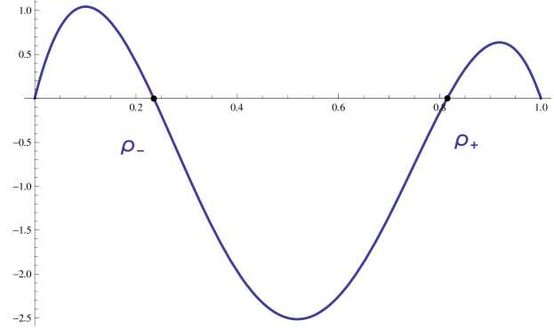
Figure 1: The potential energy profile, $E_{P}(\rho)$, is shown for a set of typical values of the parameters $\lambda$, $H$, $\mu$ and $\rho_{0}$.

There one can see that $E_{P}(\rho)$ vanishes at two densities $\rho_{\pm}$ given by

$$\rho_{\pm}=\frac{2\lambda+\mu\pm\sqrt{8\lambda({\mathcal{H}}-\mu\rho_{0})+(2\lambda+\mu)^{2}}}{4\lambda}$$ (15)

The particle thus oscillates between these two extreme positions, and it takes a full period

$$\int_{0}^{1}\textnormal{d}x=1=2\int_{\rho_{-}}^{\rho_{+}}{\textnormal{d}\rho}\frac{1}{\sqrt{-2E_{P}(\rho)}}$$ (16)

to do the round-trip between $\rho_{-}$ and $\rho_{+}$. Besides, we must have that the total density is $\rho_{0}$, which in turn imposes

$$\rho_{0}=\int_{0}^{1}\textnormal{d}x\rho(x)=2\int_{\rho_{-}}^{\rho_{+}}{\textnormal{d}\rho}\frac{\rho}{\sqrt{-2E_{P}(\rho)}}$$ (17)

The two equations (16) together with (17) thus completely fix the unknowns $\mathcal{H}$ and $\mu$. At this stage, it is more convenient to deal with the $\rho_{0}=1/2$ case, for which analytic expressions are somewhat simpler.

3.3.1 At half-filling

Particle-hole symmetry at $\rho_{0}=1/2$ imposes that $E_{P}(\rho)=E_{P}(1-\rho)$, which in turn forces $\mu=0$ (this can explicitly be verified from (16) and (17)). Then we have that

$$0<\rho_{-}=\frac{\lambda-\sqrt{\lambda(2{\mathcal{H}}+\lambda)}}{2\lambda}<\rho_{+}=\frac{\lambda+\sqrt{\lambda(2{\mathcal{H}}+\lambda)}}{2\lambda}<1$$ (18)

The density profile thus evolves between $\rho_{-}$ and $\rho_{+}$ given above, with the constant $\mathcal{H}$ being given by the implicit solution to

$$\frac{1}{2}=\frac{(\sqrt{2\mathcal{H}+\lambda}-\sqrt{\lambda})\mathop{\textnormal{K}}\left(\frac{2\sqrt{\lambda(2\mathcal{H}+\lambda)}}{\mathcal{H}+\lambda+\sqrt{\lambda(2\mathcal{H}+\lambda)}}\right)}{\sqrt{2}\mathcal{H}}$$ (19)

where $\mathop{\textnormal{K}}$ is the complete elliptic integral of the first kind. Using that as $u\to 0$

$$\mathop{\textnormal{K}}(1-u)=2\ln 2-\frac{1}{2}\ln u+\frac{u}{8}(-\ln u-2+4\ln 2)+{\mathcal{O}}(u^{2})$$ (20)

we can solve for $\mathcal{H}$ as a function of $\lambda$ from (19), which leads to

$$\mathcal{H}= 8\lambda\textnormal{e}^{-\sqrt{\frac{\lambda}{2}}}+16\textnormal{e}^{-2\sqrt{\frac{\lambda}{2}}}\lambda\big{(}\sqrt{2\lambda}-4\big{)}$$ (21)

$$\quad+16\textnormal{e}^{-3\sqrt{\frac{\lambda}{2}}}\lambda(6\lambda-19\sqrt{2\lambda}+22)+{\mathcal{O}}\left(\lambda^{3/2}\textnormal{e}^{-4\sqrt{\frac{\lambda}{2}}}\right)$$

The large deviation function $\phi(\lambda)$ is then obtained from

$$\phi(\lambda) =-\int_{0}^{1}\textnormal{d}x\left[\frac{(\partial_{x}\rho)^{2}}{2\sigma}+\lambda\sigma+(\rho-\rho_{0})\mu\right]$$ (22)

$$=\int_{0}^{1}\textnormal{d}x\left[\mathcal{H}-\frac{(\partial_{x}\rho)^{2}}{\sigma}\right]$$ (23)

Given that we have

$$\int_{0}^{1}\textnormal{d}x\frac{(\partial_{x}\rho)^{2}}{\sigma}=2\int_{\rho_{-}}^{\rho_{+}}\textnormal{d}\rho\frac{\sqrt{-2E_{P}}}{\sigma}$$ (24)

we arrive, after some manipulations, at

$$\phi(\lambda)=-{\sqrt{2}}\big{(}\sqrt{2\mathcal{H}+\lambda}+\sqrt{\lambda}\big{)}\mathop{\textnormal{E}}\left(\frac{2\sqrt{\lambda(2\mathcal{H}+\lambda)}}{\mathcal{H}+\lambda+\sqrt{\lambda(2\mathcal{H}+\lambda)}}\right)$$ (25)

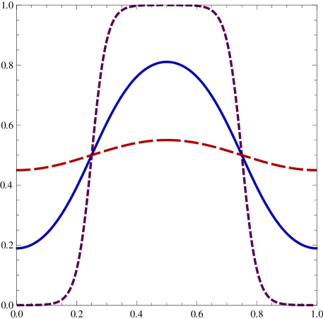
Figure 2: The density profile is shown for $\lambda=\lambda_{c}+\frac{1}{10}$ (red, large dashes), $25$ (blue), $200$ (purple, small dashes) at average density $\rho_{0}=\frac{1}{2}$. The kink becomes steeper as $\lambda$ is increased. The slope of the rise to the plateau increases as $\sqrt{\lambda}$ for large $\lambda$.

where $\mathcal{H}$ as a function of $\lambda$ is extracted from the implicit formula (19). The notations $\mathop{\textnormal{K}}$ and $\mathop{\textnormal{E}}$ refer to the complete elliptic integrals of the first and second kind, respectively. This expression is valid for any $\lambda>\lambda_{c}$. Using the following asymptotic formula for $E$ as $u\to 0$

$$\mathop{\textnormal{E}}(1-u) =1+u\left(-\frac{1}{4}\ln u-\frac{1}{4}+\ln 2\right)$$ (26)

$$\qquad+\frac{u^{2}}{64}\left(-6\ln u-13+24\ln 2\right)+{\mathcal{O}}(u^{3})$$

we arrive at the following large $\lambda$ asymptotics for $\phi(\lambda)$:

$$\phi(\lambda)= -2\sqrt{2\lambda}-8\sqrt{2\lambda}\textnormal{e}^{-\sqrt{\frac{\lambda}{2}}}$$ (27)

$$\quad+8\big{(}2\lambda-3\sqrt{2\lambda}\big{)}\textnormal{e}^{-2\sqrt{\frac{\lambda}{2}}}+{\mathcal{O}}\left(\lambda^{\frac{3}{2}}\textnormal{e}^{-3\sqrt{\frac{\lambda}{2}}}\right)$$

This is the final result for the $\rho_{0}=1/2$ particular case. Translated into the language of quantum spin chains, $\phi(\lambda)$ in (25) is the ground-state energy per site of a ferromagnetic $XXZ$ chain with anisotropy parameter $\Delta=1+\frac{\lambda}{L^{2}}$ for $\lambda>\lambda_{c}$, and at half-filling. To our knowledge, this is the first appearance of this expression in the literature. The optimal profile corresponding to that value of $\phi(\lambda)$ takes the form of a smooth kink with area equal to $1/2$, as shown in figure 2 for increasing values of $\lambda$. Its expression reads (for $x$ as function of $\rho$ for $0\leq x\leq\frac{1}{2}$)

$$x(\rho)=\frac{1}{2}-\frac{\sqrt{2}\mathop{\textnormal{F}}\Big{(}\frac{1}{2}\arccos\left(\frac{(\rho-1)\lambda-H}{(1-\rho)\sqrt{\lambda(2H+\lambda)}}\right)\Big{|}\frac{2\sqrt{\lambda(2H+\lambda)}}{H+\lambda+\sqrt{\lambda(2H+\lambda)}}\Big{)}}{\sqrt{2H+\lambda}+\sqrt{\lambda}}$$ (28)

where $\mathop{\textnormal{F}}$ is the incomplete elliptic integral of the first kind.

3.3.2 At arbitrary density $\rho_{0}$

For general $\rho_{0}$, by exactly the same methods, though with somewhat less elegant simplifications (no symmetry enforces the Lagrange multiplier $\mu$ to vanish), the two equations (16) and (17) now take the following forms

$$\frac{1}{2}\rho_{0}=\frac{2\lambda\mathop{\textnormal{K}}\Big{(}\frac{\mu+2\lambda(1-2\hat{\rho})}{(\mu+2\lambda(1-\hat{\rho}))(1-\hat{\rho})}\Big{)}+(\mu-2\lambda\hat{\rho})\Pi\Big{(}\frac{\mu+2\lambda(1-2\hat{\rho})}{2\lambda(1-\hat{\rho})}\Big{|}\frac{\mu+2\lambda(1-\hat{\rho})}{(\mu+2\lambda(1-\hat{\rho}))(1-\hat{\rho})}\Big{)}}{2\lambda\sqrt{(1-\hat{\rho})(\mu+2\lambda(1-\hat{\rho}))}}$$ (29)

where $\Pi$ is the complete elliptic integral of the third kind, along with

$$\frac{1}{2}=\sqrt{\frac{1}{(1-\hat{\rho})(2\lambda(1-\hat{\rho})+\mu)}}\mathop{\textnormal{K}}\left(\frac{\mu+2\lambda(1-2\hat{\rho})}{(\mu+2\lambda(1-\hat{\rho}))(1-\hat{\rho})}\right)$$ (30)

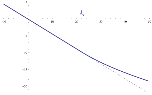
Figure 3: Large deviation function $\phi(\lambda)$ (thick line) as a function of $\lambda$, at average density $\rho_{0}=\frac{2}{3}$. The function is singular at $\lambda=\lambda_{c}=\frac{\pi^{2}}{\sigma(\rho_{0})}$ (the second derivative is discontinuous), marking the entrance in the regime where the density profile is non-uniform ($\lambda>\lambda_{c}$). The value of the large deviation function for a uniform profile at $\lambda>\lambda_{c}$ is shown for comparison (dashed line).

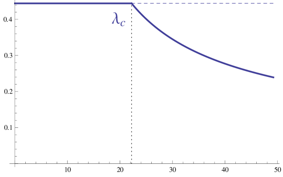
Figure 4: Mean activity $\frac{1}{Lt}\langle K\rangle_{\lambda}=-\phi^{\prime}(\lambda)$ (thick blue line) as a function of $\lambda$, at average density $\rho_{0}=\frac{2}{3}$. The function is singular at $\lambda=\lambda_{c}=\frac{\pi^{2}}{\sigma(\rho_{0})}$. The value of $\frac{1}{Lt}\langle K\rangle_{s}$ is shown for a uniform profile at $\lambda>\lambda_{c}$ is shown for comparison (dashed line). As expected, above $\lambda_{c}$, the activity for histories with a non-uniform profile is lower than for uniform profiles.

where $\hat{\rho}$ is either equal to the minimum or the maximum density $\rho_{\pm}$ [defined in (15)]. Once $\mu$ and $\mathcal{H}$ have been extracted from (29) and (30), one can determine the large deviation function $\phi(\lambda)$ as a function of $\lambda$ and $\rho_{0}$ from the formula (see figures 3 and 4)

$$\phi(\lambda) =-2\sqrt{(1-\hat{\rho})(2\lambda(1-\hat{\rho})+\mu)}\mathop{\textnormal{E}}\left(\frac{\mu+2\lambda(1-2\hat{\rho})}{(\mu+2\lambda(1-\hat{\rho}))(1-\hat{\rho})}\right)$$ (31)

where $\lambda>\lambda_{c}$.The expansion close to $\lambda_{c}$ can be checked from those results. We see in particular that $\frac{1}{L^{3}t}\langle K^{2}\rangle_{c}=\phi^{\prime\prime}(\lambda)$ presents a jump $\phi^{\prime\prime}(\lambda_{c}^{+})-\phi^{\prime\prime}(\lambda_{c}^{-})=\frac{6\sigma(\rho_{0})^{3}}{\pi^{2}}$. We do not intend to labour beyond the leading order of $\phi(\lambda)$ as $\lambda\gg 1$, which is independent of $\rho_{0}$,

$$\phi(\lambda)\simeq-2\sqrt{2\lambda}+\mathcal{H}+(1-\rho_{0})\mu+\ldots$$ (32)

That the leading contribution is independent of $\rho_{0}$ could have been expected, as the main contribution to $\phi$ as given in (23) is the integral (24), which is itself dominated by a small region of size $1/\sqrt{\lambda}$ where the derivative of $\rho$ varies the most steeply between $\rho_{-}$ and $\rho_{+}$, while density is close to $\frac{\rho_{-}+\rho_{+}}{2}\simeq 1/2$, and thus

$$\phi(\lambda)\sim-\left({1}/{\sqrt{\lambda}}\right)\times\frac{1}{1/\sqrt{\lambda}^{2}}\sim-\sqrt{\lambda}$$ (33)

Together with the implicit formulas (29) and (30), equation (31) is the ground state energy of an $XXZ$ ferromagnetic Heisenberg chain with anisotropy parameter $\Delta=1+\frac{\lambda}{L^{2}}$ at fixed magnetization $L(2\rho_{0}-1)$. The density profile is, for $x$ as function of $\rho$ for $0\leq x\leq\frac{1}{2}$ (see figure 5),

$$x(\rho)=\frac{\mathop{\textnormal{F}}\Big{(}\arcsin\Big{(}\sqrt{\frac{(\mu-2\lambda\rho_{-})(\rho-\rho_{-})}{(2(2\rho_{-}-1)\lambda-\mu)(1-\rho)}}\Big{)}\Big{|}\frac{2\lambda(1-2\rho_{-})+\mu}{(\mu-2\lambda\rho_{-})\rho_{-}}\Big{)}}{\sqrt{\rho_{-}(2\lambda\rho_{-}-\mu)}}$$ (34)

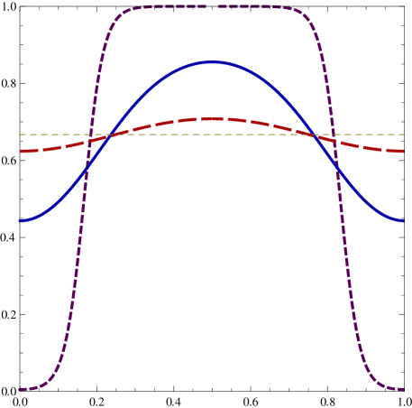
Figure 5: The density profile is shown for $\lambda=\lambda_{c}+\frac{1}{10}$ (red, large dashes), $25$ (blue), $200$ (purple, small dashes) at average density $\rho_{0}=\frac{2}{3}$ (thin dashes). The kink becomes steeper as $\lambda$ is increased.

3.4 The infinitely inactive regime

In the infinitely inactive regime, that is for $\lambda\gg L^{2}$, the density profile described in the previous subsections becomes infinitely steep and the assumptions underlying fluctuating hydrodynamics fail. Since the typical slope of the rise of the profile towards its plateau value increases at $\sqrt{\lambda}$, fluctuating hydrodynamics must fail when the slope exceeds $L$, that is when profile variations become significant at the lattice scale, which is consistent with the $\lambda\gg L^{2}$ condition. For large $s$ it is easy to see that the ground state of the $s$-modified evolution operator (1) reads

$$\psi(s)=-2L\sigma(\rho_{0})(1-\textnormal{e}^{-s})+O(\textnormal{e}^{-2s})$$ (35)

The above regime consistently connects to the calculation of the previous subsection where it was shown that $\phi(\lambda)\sim-\sqrt{\lambda}$ for large values of $\lambda$. The validity of that previous result holds until $\phi(\lambda)\sim-2L\sigma(\rho_{0})$, when it connects with the infinitely inactive regime. This occurs as $\lambda\sim L^{2}$ and confirms once more that the crossover is at a typical $\lambda$ of the order of $L^{2}$.

4 Prospects

The SSEP on a ring displays a phase transition from a homogeneous state to a kink-like profile as the trajectories’ activity is lowered below its average value. We have described both the details of the kink profile that develops and the large deviation function of the activity itself in this nonuniform dynamical state. In the course of our analysis, we have identified three distinct finite-size scaling regimes. The system dealt with in the present work exhibits a second order continuous phase transition. It would certainly be quite desirable to find similar solvable examples for first-order transitions. The mechanism by which the symmetry breaking sets in may be more subtle. This is work in progress.

Acknowledgements

We would like to thank Thierry Giamarchi for interesting discussions on $XXZ$ related matters. This work was supported in part by British Council France Alliance Project 09.013.

References

References

- [1] Julien Tailleur, Jorge Kurchan, and Vivien Lecomte. Mapping Nonequilibrium onto Equilibrium: The Macroscopic Fluctuations of Simple Transport Models. Phys. Rev. Lett. 99, 150602 (2007).
- [2] Julien Tailleur, Jorge Kurchan, and Vivien Lecomte. Mapping out-of-equilibrium into equilibrium in one-dimensional transport models. J. Phys. A 41, 505001 (2008).
- [3] A. Imparato, V. Lecomte, and F. van Wijland. Equilibriumlike fluctuations in some boundary-driven open diffusive systems. Phys. Rev. E 80, 011131 (2009).
- [4] Vivien Lecomte, Alberto Imparato, and Frédéric van Wijland. Current Fluctuations in Systems with Diffusive Dynamics, in and out of Equilibrium. Prog. Theor. Phys. Suppl. 184, 276 (2010).
- [5] Thierry Bodineau and Bernard Derrida. Distribution of current in nonequilibrium diffusive systems and phase transitions. Phys. Rev. E 72, 066110 (2005).
- [6] Thierry Bodineau and Bernard Derrida. Cumulants and large deviations of the current through non-equilibrium steady states. C. Rendus Physique 8, 540 (2007).
- [7] Juan P. Garrahan, Robert L. Jack, Vivien Lecomte, Estelle Pitard, Kristina van Duijvendijk, and Frédéric van Wijland. Dynamical First-Order Phase Transition in Kinetically Constrained Models of Glasses. Phys. Rev. Lett. 98, 195702 (2007).
- [8] Juan P. Garrahan, Robert L. Jack, Vivien Lecomte, Estelle Pitard, Kristina van Duijvendijk, and Frédéric van Wijland. First-order dynamical phase transition in models of glasses: an approach based on ensembles of histories. J. Phys. A 42, 075007 (2009).
- [9] Lorenzo Bertini, Alberto De Sole, Davide Gabrielli, Giovanni Jona-Lasinio, and Claudio Landim. Current Fluctuations in Stochastic Lattice Gases. Phys. Rev. Lett. 94, 030601 (2005).
- [10] Lorenzo Bertini, Alberto De Sole, Davide Gabrielli, Giovanni Jona-Lasinio, and Claudio Landim. Non Equilibrium Current Fluctuations in Stochastic Lattice Gases. J. Stat. Phys. 123, 237 (2006).
- [11] Christian Beck and Friedrich Schlögl. Thermodynamics of chaotic systems: an introduction. Cambridge University Press 1995.
- [12] Thierry Bodineau and Cristina Toninelli. Activity phase transition for constrained dynamics. arXiv:1101.1760 accepted for publication in Comm. Math. Phys. (2011).
- [13] Thierry Bodineau, Vivien Lecomte, and Cristina Toninelli. Finite size scaling of the dynamical free-energy in a kinetically constrained model. arXiv:1111.6394 (2011).
- [14] Vivien Lecomte, Cécile Appert-Rolland, and Frédéric Wijland. Thermodynamic Formalism for Systems with Markov Dynamics. J. Stat. Phys. 127, 51 (2007).
- [15] Mauro Merolle, Juan P. Garrahan, and David Chandler. Space-time thermodynamics of the glass transition. PNAS 102, 10837 (2005).
- [16] Thierry Bodineau and Raphaël Lefevere. Large Deviations of Lattice Hamiltonian Dynamics Coupled to Stochastic Thermostats. J. Stat. Phys. 133, 1 (2008).
- [17] Lester O. Hedges, Robert L. Jack, Juan P. Garrahan, and David Chandler. Dynamic Order-Disorder in Atomistic Models of Structural Glass Formers. Science 323, 1309 (2009).
- [18] Estelle Pitard, Vivien Lecomte, and Frédéric Van Wijland. Dynamic transition in an atomic glass former: a molecular dynamics evidence. Europhys. Lett. 96, 184207 (2011).
- [19] Christian Maes, Karel Netočný, and Bram Wynants. On and beyond Entropy Production: the Case of Markov Jump Processes. Markov Proc. Rel. Fields 14, 445 (2008).
- [20] Cécile Appert-Rolland, Bernard Derrida, Vivien Lecomte, and Frédéric van Wijland. Universal cumulants of the current in diffusive systems on a ring. Phys. Rev. E 78, 021122 (2008).
- [21] Rodney Baxter. Exactly solved models in statistical mechanics. Academic Press London ;;New York 1982.
- [22] Elliott H Lieb and Werner Liniger. Exact Analysis of an Interacting Bose Gas. I. The General Solution and the Ground State. Phys. Rev. 130, 1605 (1963).
- [23] Michel Gaudin. La fonction d’onde de Bethe. Masson Paris New York 1983.
- [24] Mehran Kardar. Replica Bethe Ansatz studies of two-dimensional interfaces with quenched random impurities. Nucl. Phys. B 290, 582 (1987).
- [25] Pasquale Calabrese, Pierre Le Doussal, and Alberto Rosso. Free-energy distribution of the directed polymer at high temperature. EPL (Europhysics Letters) 90, 20002 (2010).
- [26] Victor Dotsenko. Bethe ansatz derivation of the Tracy-Widom distribution for one-dimensional directed polymers. Europhys. Lett. 90, 20003 (2010).
- [27] Ivan Corwin. The Kardar-Parisi-Zhang equation and universality class. arXiv:1106.1596 2011.
- [28] Giuseppe Albertini, Vladimir E. Korepin, and Andreas Schadschneider. XXZ model as an effective Hamiltonian for generalized Hubbard models with broken eta-symmetry. J. Phys. A 28, L303 (1995).
- [29] Lorenzo Bertini, Alberto De Sole, Davide Gabrielli, Giovanni Jona-Lasinio, and Claudio Landim. Fluctuations in Stationary Nonequilibrium States of Irreversible Processes. Phys. Rev. Lett. 87, 040601 (2001).
- [30] Lorenzo Bertini, Alberto De Sole, Davide Gabrielli, Giovanni Jona-Lasinio, and Claudio Landim. Macroscopic Fluctuation Theory for Stationary Non-Equilibrium States. J. Stat. Phys. 107, 635 (2002).
- [31] Lorenzo Bertini, Alberto De Sole, Davide Gabrielli, Giovanni Jona-Lasinio, and Claudio Landim. Large Deviations for the Boundary Driven Symmetric Simple Exclusion Process. Math. Phys. Analysis and Geometry 6, 231 (2003).
- [32] Claude Kipnis and Claudio Landim. Scaling Limits of Interacting Particle Systems. Springer softcover reprint of hardcover 1st ed. 1999 edition 2010.
- [33] Thierry Bodineau and Bernard Derrida. Current Fluctuations in Nonequilibrium Diffusive Systems: An Additivity Principle. Phys. Rev. Lett. 92, 180601 (2004).