Fixed-points in Random Boolean Networks:
The impact of parallelism in the scale-free topology case

Abstract

Fixed points are fundamental states in any dynamical system. In the case of gene regulatory networks (GRNs) they correspond to stable genes profiles associated to the various cell types. We use Kauffman’s approach to model GRNs with random Boolean networks (RBNs). We start this paper by proving that, if we fix the values of the source nodes (nodes with in-degree 0), the expected number of fixed points of any RBN is one (independently of the topology we choose). For finding such fixed points we use the $\alpha$-asynchronous dynamics (where every node is updated independently with probability $0<\alpha<1$). In fact, it is well-known that asynchrony avoids the cycle attractors into which parallel dynamics tends to fall. We perform simulations and we show the remarkable property that, if for a given RBN with scale-free topology and $\alpha$-asynchronous dynamics an initial configuration reaches a fixed point, then every configuration also reaches a fixed point. By contrast, in the parallel regime, the percentage of initial configurations reaching a fixed point (for the same networks) is dramatically smaller. We contrast the results of the simulations on scale-free networks with the classical Erdös-Rényi model of random networks. Everything indicates that scale-free networks are extremely robust. Finally, we study the mean and maximum time/work needed to reach a fixed point when starting from randomly chosen initial configurations.

1 Introduction

A Random Boolean Network (RBN) is a model of a GRN. This model was introduced by Kauffman in 1969 [26] and it corresponds to a directed graph composed by $N$ genes (nodes) where each of these genes can be either expressed (state 1) or not expressed (state 0). Each gene $v$ receives $K$ randomly chosen genes as input ($K$ nodes pointing to $v$). In other words, the dynamics is defined locally. The idea of Kauffman was to choose, independently for each node $v$, any of the $2^{2^{K}}$ possible functions $f_{v}:\{0,1\}^{K}\to\{0,1\}$ with equal probability. Finally, a global dynamics $f:\{0,1\}^{N}\to\{0,1\}^{N}$ was defined by applying the local functions in parallel (sometimes this is referred to as synchronous updates). Kauffman found, through simulations, the existence of a phase transition at $K=K_{c}=2$ (from an ordered phase to a chaotic phase). He also suggested that the number of attractors grows exponentially with $N$ in the chaotic phase, proportional to $N$ in the ordered phase, and proportional to $\sqrt{N}$ at the critical value $K_{c}=2$.

Kauffman’s model (and some natural generalizations) motivated a lot of work carried out mainly by physicists. They tackled problems arising from Kauffman’s definitions both analytically and numerically: the critical in-degree value [8, 16], the number of attractors [11, 16], the length distribution of the attractors [4, 10], etc.

From the biologists point of view a fundamental challenge of the post-genomic era is the possibility of simulating the dynamics of real genetic networks. The enormous amount of available data of molecular interactions within the cell made it possible to examine critically the original RBN model. The first observation was that the topology assumption was inadequate. Contrasting the uniform topology assumed in the original RBNs, it has been shown that real genetic networks exhibit a scale-free topology [3, 12, 20, 28]. In such topologies a small fraction of the genes are highly connected whereas the majority of the genes are poorly connected [1, 30]. Therefore, RBNs dynamics with scale-free topology started to be intensively studied [5, 13, 24].

Another criticism towards Kauffman’s model was that nodes were updated in parallel. Experimental results confirmed a rather intuitive fact: that genes transition between expressed and non-expressed states at different times [15, 17]. Informally, there is no global clock that allows transition to happen only at ticks. Therefore, RBNs with scale-free topology and asynchronous dynamics is a natural model to be analyzed [14]. We would also like to point out that asynchrony in the classical RBN model has also been studied in [21, 22, 27] and [29].

Our main contributions. Fixed points are fundamental states in any dynamical system. In the case of GRNs they correspond to stable gene expression profiles associated to the various cell types. This interpretation has been used for modeling europhil differentiation [23], expression patterns of the segment polarity genes in Drosophila melanogaster [2], flower organ specification in Arabidopsis thaliana [6], etc.

The goal of this paper is to study the of existence fixed points in RBNs with scale-free topology. Notice that a fixed point does not depend on the timing (synchronous/asynchronous) of the update rule. In fact, in a fixed point every gene is in a stable state with respect to its local input. Therefore, there is no way to change such global configuration. In that sense, a fixed point is a very robust object of a network, despite the fact that its basin of attraction can change depending on how the update rule is implemented.

Once the topology of the network is (randomly) generated some nodes will have only outgoing arcs. These were called source nodes by Albert [3] and we will use the same terminology here. Since their states do not depend on the state of any other node we fix their values arbitrarily. In this paper we prove that, for every given assignment to the input nodes, the expected number of fixed points is exactly one (for every topology).

Now the main (and natural) question arises. Given a RBN, how can we actually find its fixed points? It is clear that testing all the $2^{N}$ configurations is impossible. For answering the question we come back to the issue of asynchrony. In fact, in 1994 Bersini and Detours studied an asynchronous version of the cellular automaton Game-of-Life [9]. They observed that the introduction of asynchrony modified the dynamics from a behavior with long transients to a behavior with fixed points. This is rather intuitive: asynchrony is a way to avoid the cycle attractors the deterministic (parallel) implementation tend to fall into.

Therefore, the strategy is clear. Given a RBN, we implement the $\alpha$-asynchronous dynamics for different values of $\alpha$ ($0\leq\alpha\leq 1$)  [19]. Roughly, this means that, at each time step, each gene is updated independently with probability $\alpha$. When $\alpha$ varies from 1 down to 0 the dynamics evolves from the fully deterministic synchronous regime to a more asynchronous regime. When $\alpha=0$ we choose randomly only one node at each step.

Our simulations show that RBNs with scale-free topology for which there exist a fixed points every initial configuration converges to a fixed point when $0\leq\alpha<1$. On the other hand, when $\alpha=1$, the percentage of initial configurations that reached a fixed point varies greatly form one network to another. In some cases the percentage is close to 0. In average (considering all the networks we use) the percentage is $\sim$28.9%.

In order to find properties which could be associated exclusively to the topology of the network we compare the results of the simulations on scale-free networks with the results on the classical Erdös-Rényi model of random networks [18]. The main difference with the scale-free topology is that here we generated networks for which the percentage of initial configurations converging to a fixed point is close to $0$. Finally, we study the mean and maximum time/work needed to reach a fixed point when starting from randomly chosen initial configurations.

Therefore, a remarkable and distinguishable dynamical property arise on RBNs with scale-free topology: robustness of convergence under asynchronous update. This fact could provide some insight about why such topologies are ubiquitous in GRN. Furthermore, asynchronous updating could be a natural mechanism present in GRNs in order to avoid cyclic dynamics [29].

2 Network model

A Random Boolean Network (RBN) corresponds to a directed graph composed by $N$ genes (nodes) where each of these genes can be either expressed (state 1) or not expressed (state 0). We will refer to the nodes of a RBN as $v_{1},v_{2},\ldots,v_{N}$. We define $K_{i}^{in}$ as the in-degree of node $v_{i}$ and $K_{i}^{out}$ as the out-degree of node $v_{i}$. Every zero in-degree node is called a source node, while every non-zero in-degree node is called an internal node. A configuration of the network is a vector ${\mathbf{s}}\in\{0,1\}^{N}$ that associates a binary state to each of the nodes.

2.1 Dynamics

We assign to each gene $v_{i}$ a local transition rule $\phi_{i}:\{0,1\}^{K_{i}^{in}+1}\rightarrow\{0,1\}$. Informally, the value of $\phi_{i}$ depends on the state of the $K_{i}^{in}$ input nodes together with the state of $v_{i}$ itself. source nodes always remain in the same state. More precisely, if $K^{in}_{i}=0$, then $\phi_{i}(0)=0$ and $\phi_{i}(1)=1$. For each internal node $v_{i}$ we construct randomly its local transition function as follows. Call $k$ the in-degree of $v_{i}$ (i.e, $k=K^{in}_{i}$). There are $2^{2^{k}}$ possible functions of the form $f:\{0,1\}^{k}\rightarrow\{0,1\}$. A straightforward approach is to choose one of these functions from a uniform probability distribution. Nevertheless, before selecting a function, we should rule out those which do not strictly depend on all of its arguments (otherwise we would not be respecting the network topology). To define this concept precisely, we say that a function $f:\{0,1\}^{k}\rightarrow\{0,1\}$ strictly depends on its arguments iff for all $j\in\{1,2,\cdots,k\}$, there exist $x_{1},x_{2},\cdots,x_{j-1},x_{j+1},\cdots,x_{k}\in\{0,1\}$ such that $f(x_{1},x_{2},\cdots,x_{j-1},0,x_{j+1},\cdots,x_{k})\not=f(x_{1},x_{2},\cdots,x_{j-1},1,x_{j+1},\cdots,x_{k})$. We fix function $\phi_{i}$ by selecting one (randomly) among all those functions strictly depending on all of its arguments.

The global update rule is characterized by a real parameter $\alpha\in[0,1]$. We denote the global transition rule by $\mathbf{\Phi}_{\alpha}:\{0,1\}^{N}\rightarrow\{0,1\}^{N}$, and we define it through the following protocol:

1. Select each internal node independently with probability $\alpha$. We call selected nodes this set of randomly chosen internal nodes. For the special case $\alpha=0$ we select randomly a single internal node (i.e, the set of selected nodes is a singleton).

2. Update in parallel all the selected nodes (applying the local transition rule in all the nodes belonging to such set). Do not change the state of the other nodes (input nodes and non-selected nodes).

Let ${\mathbf{s}}_{t}\in\{0,1\}^{N}$ be a configuration of a RBN at time $t\in\mathbb{N}$. A stochastic trajectory, starting from the initial configuration ${\mathbf{s}}_{0}$, is the sequence ${\mathbf{s}_{0}},{\mathbf{s}_{1}},{\mathbf{s}_{2}},\ldots$, where ${\mathbf{s}_{i}}={\mathbf{\Phi}}_{\alpha}({\mathbf{s}_{i-1}})$.

The parameter $\alpha$ can be thought of as a measure of parallelism in the update process. The strictly sequential-random policy rule is captured by $\alpha=0$, where only one internal node is updated at each step. Similarly, by making $\alpha=1$, we represent the full parallel-deterministic policy rule, where all the internal nodes are updated at each step. If $\alpha=1$ we call the resulting trajectory the deterministic trajectory of the system. A configuration $\mathbf{s}$ is a fixed point of a RBN iff $\Pr\{\mathbf{\Phi}_{\alpha}(\mathbf{s})=\mathbf{s}$}=1. This is equivalent to say that $\mathbf{\Phi}_{1}(\mathbf{s})=\mathbf{s}$. Therefore, $\mathbf{s}$ is a fixed point regardless of the choice of $\alpha$.

We measure time simply by counting the applications of $\mathbf{\Phi}_{\alpha}$. Therefore, the time to go from ${\mathbf{s}_{0}}$ to ${\mathbf{s}_{T}}$ in a trajectory is $T$. This notion of time neglects the fact that the computational effort to evaluate $\mathbf{\Phi}_{\alpha}$ depends on $\alpha$. The expected number of $\phi$’s to be evaluated is $\alpha N_{I}$ where $N_{I}$ is the number of internal nodes. Thus, we define the work to go from state ${\mathbf{s}_{0}}$ to ${\mathbf{s}_{T}}$ to be $\alpha T$ for all $\alpha>0$. For the special case $\alpha=0$ we define the work as $\frac{1}{N_{I}}T$.

When considering the dynamics of the network with $\alpha=1$, it is clear that the trajectory will eventually become cyclic. Note that if the system reaches a fixed point, the length of the period is 1. Both the time to enter the cycle and the period are bounded by $2^{N_{I}}$, where $N_{I}$ is the number of internal nodes. However, if $\alpha<1$, the idea of cycle is insufficient to describe a trajectory that does not reach a fixed point. Instead, we have a set of configurations which are visited infinitely often. This greatly complicates the numerical determination of any eventual convergence to a fixed point. We therefore select a somewhat arbitrary time horizon to interrupt our simulations.

Notice that, given an initial configuration $\mathbf{s}_{0}$, the set of configurations reachable from $\mathbf{s}_{0}$ by repeated applications of $\mathbf{\Phi}_{1}$ is a subset of the set of configurations potentially reachable from $\mathbf{s}_{0}$ by repeated applications of $\mathbf{\Phi}_{\alpha}$ when $\alpha<1$. In other words, the stochastic trajectory can visit a larger portion of the state space than the deterministic one.

A remarkable feature of selecting the local update functions randomly, as we did, is that we can predict, in a statistical sense, the number of fixed points in the network. Consider an arbitrary configuration $\mathbf{s}\in\{0,1\}^{N}$. What is the probability of $\mathbf{s}$ to be a fixed-point? First notice that $\mathbf{s}$ is a fixed point if and only if $\mathbf{s}_{i}=\phi_{i}({\mathbf{s}}_{i_{1}},\ldots,{\mathbf{s}}_{i_{k_{i}}})$ for every $i\in\{1,\ldots,N\}$, where $v_{i_{1}},\ldots,v_{i_{k_{i}}}$ are the input nodes of $v_{i}$.

It follows from the definition of the $\phi_{i}$’s functions, that $\Pr\{\phi_{i}({\mathbf{s}}_{i_{1}},\ldots,{\mathbf{s}}_{i_{k}})=0\}=\Pr\{\phi_{i}({\mathbf{s}}_{i_{1}},\ldots,{\mathbf{s}}_{i_{k}})=1\}=\frac{1}{2}$ for every internal node $v_{i}$. The reason for that is the following: if a function $\phi_{i}$ strictly depends on all of its arguments then the complementary function (the one where we replace 1’s with 0’s and 0’s with 1 s) also does. On the other hand, $\Pr\{\phi_{i}({\mathbf{s}}_{i})={\mathbf{s}}_{i}\}=1$ for every source node $v_{i}$. Therefore, the probability of $\mathbf{s}$ to be a fixed-point is $2^{-{N_{I}}}$, where $N_{I}$ is the number of internal nodes.

Let $X_{\mathbf{s}}$ be the Boolean random variable that equals 1 if the configuration $\mathbf{s}$ is a fixed point and 0 otherwise. The expected number of fixed points is

$$\sum_{\mathbf{s}\in\{0,1\}^{N}}{\mathbbm{E}(X_{\mathbf{s}})}=\sum_{\mathbf{s}\in\{0,1\}^{N}}2^{-{N_{I}}}=2^{N-N_{I}}$$

Note that $N-N_{I}=N_{E}$ is the total number of source nodes of the network. If we fix all these source nodes to some arbitrary value in the initial configuration, then the expected number of fixed points goes down to 1. In fact, in that case, the number of effective different configurations is $2^{N-N_{E}}=2^{N_{I}}$ and the expected number of fixed points becomes $2^{N_{I}-N_{I}}=1$ instead of the original $2^{N-N_{I}}$.

Until this point, neither the definitions nor the theorem we just proved make assumptions about the topology of the RBN. In the following subsection we will describe two families of topologies that have been studied in the literature.

2.2 Topology

We start describing here a process by which we construct a directed scale-free network with $N$ nodes and average in/out-degree equal to $k$. Let $N_{0}$ and $k$ be positive integers such that $k\leq N_{0}\leq N$. The process starts from a directed clique with $N_{0}$ nodes (i.e, $N_{0}(N_{0}-1)$ arcs). Call these nodes $v_{1},v_{2},\ldots,v_{N_{0}}$. The process now involves $N-N_{0}$ growth stages, numbered $N_{0}+1,N_{0}+2,\ldots,N$. At each stage, a single node is added to the network.

Call $v_{i}$ the node added at stage $i$. We will also add $k$ edges to the growing network. We toss a fair coin and proceed as follows:

1. In the case of heads we add $k$ edges pointing from $k$ different nodes in $\{v_{1},\ldots v_{i-1}\}$ towards $v_{i}$. These $k$ nodes are selected randomly following a preferential attachment rule such that the probability of $v_{j}$ to be selected is proportional to $K^{out}_{j}+1$.

2. In the case of tails we add $k$ edges pointing from $v_{i}$ to $k$ different nodes in $\{v_{1},\ldots v_{i-1}\}$. These $k$ nodes are selected randomly following a preferential attachment rule, such that the probability of $v_{j}$ to be selected is proportional to $K^{in}_{j}+1$.

We will refer to the process just described as the BA algorithm because it is based on previous work by Barabási and Albert  [7]. Following [24], we started with a clique of size $N_{0}=5$ and average in/out-degree $k=2$ to create the topology using the BA method. If a RBN has a topology created by the BA algorithm, we will call it a scale-free network.

The BA method, as defined here, never creates an edge from some node to itself. The same assumption is present in [7] and [24] and is pervasive in the literature. It is noteworthy that the theorem proved in Subsection 2.1 does not require a special topology. Therefore, it still applies to networks where auto-regulation is present. Thus, for given values for the input nodes, the expected number of fixed points would still be 1. It is conceivable that the probability distribution of the number of fixed points will change, though.

In the next sections, we compare the results on scale-free networks with the classical Erdös-Rényi model of random networks [18] (random directed graphs). By doing so we intend to find properties which could be associated exclusively to the topology of the network. Random networks of this well-known Erdös-Rényi family can be easily generated. Let $p$ be a real number in the $[0,1]$ interval. Each potential link $(v_{i},v_{j})$ is selected independently with probability $p$. Therefore, the expected number of links in the Erdös-Rényi network is $pn(n-1)$, where $n$ is the number of nodes in the Erdös-Rényi network. We will call this process the ER algorithm. If a RBN has a topology created by the ER algorithm, we will call it an Erdös-Rényi network.

Conceptually, to make such comparison “fair,” we have to adjust the parameters used by the generation algorithm so the networks generated have some common statistical properties. It seems reasonable to preserve both the number of internal nodes and the average in-degree. The first parameter determines the number of states the system can be in, after the state of the source nodes have been fixed. The average in-degree is a measure of connectivity and density. Formally, if we run the topology generation BA algorithm presented for scale free networks with parameter $N$ (recall that $N_{0}=5$ and $k=2$) we will obtain a scale-free network $G_{BA}$. The average in-degree is $k=2$. Call $N_{I}$ the expected number of internal nodes of $G_{BA}$. Similarly, if we run the topology generation ER algorithm with parameters $n$ and $p$, we will obtain a graph $G_{ER}$.

The problem we wish to solve is: Given $N_{I}$ find $n$ and $p$ such that the expected in-degree of nodes in $G_{ER}$ is 2 and the expected number of internal nodes of $G_{ER}$ is $N_{I}$. Therefore,

$$p\cdot(n-1) =2$$ (1)

$$n\cdot(1-(1-p)^{n-1}) =N_{I}$$ (2)

From Eqn 1, $p=\frac{2}{(n-1)}$. Substituting in Eqn 2:

$$n\cdot\left(1-\left(1-\frac{2}{(n-1)}\right)^{n-1}\right)=N_{I}$$ (3)

The only unknown is $n$, and although this equation is hard to solve in closed form, the right hand side behaves linearly in the asymptotic sense. Using simple calculus techniques, we can estimate the solution to Eq 3 as:

$$n=\left(N_{I}-2\cdot e^{-2}\right)\frac{1}{1-e^{-2}}$$ (4)

The asymptotic approximation is so good that the rounding of $n$ to an integer is the biggest source of error even for small values, say $10$, of $N_{I}$. Therefore, for practical purposes, Eq 4 gives the exact answer. To use this formula you have to know $N_{I}$, though. In spite of $N_{I}$ being determined by $N$, it is not straightforward to find out an explicit formula. To obtain an approximation, we can simply generate a suitable number of networks using the BA algorithm and estimate $N_{I}$ as the average of the number internal nodes over all the generated graphs.

3 Simulations

We programmed a simulator using about 700 lines of portable ANSI C. We ran a number of pseudo-random experiments. The main goal was to study the influence of the parameter $\alpha$ in the dynamics of the networks. More precisely, we were interested in answering, for a given network, the following questions as a function of $\alpha$:

1. Are there fixed points?

2. If yes,

   1. how many?

   2. what fraction of trajectories converge to a fixed point?

3. If we restrict the analysis to those trajectories that converged to a fixed point,

   1. what is the average time (number of iterations) until a fixed point is reached?

   2. what is the average work (total number of operations) until a fixed point is reached?

We setup the time horizon to 50000 iterations. This number seems to yield a robust determination of whether the network eventually reaches a fixed point or not. For the scale-free networks we ran the BA algorithm using parameters $N=100$ and $k=2$. We generated $50$ networks. For each network we generated $1000$ initial configurations. The states were generated randomly, but the values corresponding to source nodes were set to zero. More precisely, to generate the initial configuration $\mathbf{s}$ of a network $N$, if $K^{in}_{i}=0$ then the $i$-th component of $\mathbf{s}$ was set to zero. Otherwise, the $i$-th component of $\mathbf{s}$ was generated randomly by tossing a fair coin.

Each one of the $50\times 1000$ pairs network/initial configuration was used as a starting point for 11 simulations, each one using a different value of $\alpha$. The values of $\alpha$ were $0,0.1,...,0.9,1$. We ran each one of the $50\times 1000\times 11$ simulations until the trajectory converged to fixed point or the time horizon was reached.

For the networks using the Erdös-Rényi topology we had to compute the input parameters for the ER algorithm ($n$ and $p$). To estimate $N_{I}$, we generated $10000$ graphs using the BA algorithm, with $k=2$ and $N=100$. Then we divided the total number of internal nodes by 10000, which yielded $N_{I}=62.745$. By using Eq 4, we determined $n=72$. From Eq 1 we obtained $p=0.028196$.

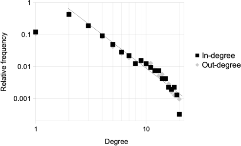
With the two parameters, we repeated the process we used for the scale-free networks: We created $50$ random networks and, for each one, we generated $1000$ initial conditions. We also used the same values for $\alpha$ and the same time horizon for the simulations. We verified that the BA algorithm indeed produces graphs with vertex degrees that follow a power law probability distribution. Figure 1 shows the relative frequency of each degree, for the 50 scale-free networks. The diagram, in log-log coordinates, shows a high similarity with a straight line. This is what we expect from a power-law distribution. The noise for the higher vertex degrees is not surprising, as highly connected vertices are rare and hence the population size is small.

Figure 1: Relative frequency of vertex degrees in the 50 scale-free networks

4 Results and analysis

4.1 Number of fixed points

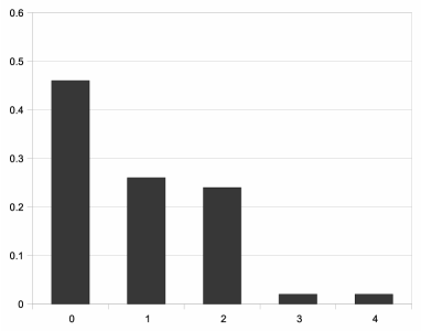
For both the scale-free and the Erdös-Rényi families we computed the number of fixed points found per each network and we summarize the results in Figures 3 and 3. The vertical axis of the histograms represent relative frequency over the 50 networks tested. Note that in 15 out of the 50 generated scale-free networks, no fixed point was found. More precisely, for all $\alpha$, none of the 1000 trajectories was absorbed into a fixed point within the 50000 iterations used as time horizon. The number of Erdös-Rényi networks for which no fixed-point was found is 23.

Figure 2: Frequency of number of fixed points for scale-free networks.

Figure 3: Frequency of number of fixed points for Erdös-Rényi networks.

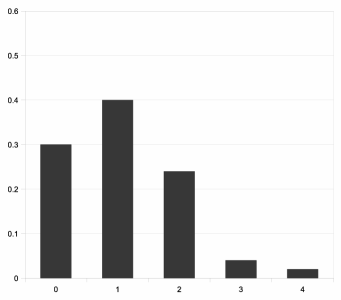
We proved analytically in Section 2 that the expected number of fixed points for any network is $1$. Unfortunately, the actual distribution is hard to compute and therefore we use histograms as a base for a numerical approximation. We can see in Figure 3 that for scale-free network the most likely number of fixed points is $1$. If we use the relative frequencies to approximate probabilities, then the estimated expected number of fixed points is $1.08$, which is close to the theoretical prediction.

By contrast, for the Erdös-Rényi model, we can see in Figure 3 that the distribution gets more skewed and $0$ becomes the most likely value. The estimation of expected number of fixed points in this case yielded $0.88$. This estimation is close to $1$ if we consider we are using only 50 networks and the number of potential fixed points is about $2^{N_{I}}$, with $N_{I}\approx 63$, as we described in Subsection 2.2.

4.2 Fraction of converging trajectories

We begin by focusing our analysis on those 35 scale-free networks for which we were able to prove the existence of fixed points (by finding them). Recall that we used 1000 initial configuration per network. If $\alpha<1$ (i.e, $\alpha=0,0.1,\ldots,0.9$) out of the 350000 stochastic trajectories we computed, 100% of them reached a fixed point. Despite the fact that for all these 35 networks we were also able to find at least one converging trajectory when $\alpha=1$, the situation in this case changed dramatically. In fact, out of the 35000 deterministic trajectories we simulated for those 35 networks, only $\sim$28.9% of them reached a fixed point. Notice also that the percentage of deterministic trajectories that reached a fixed point varied greatly form one network to another. We present the percentages for each network in Figure 5. Every single trajectory that did not reach a fixed point ended in a cycle within the time horizon. For presentation purposes, we included the analogous diagram for $\alpha<1$ in Figure 5.

Figure 4: Percentage of simulations that converged when $\alpha<1$ for each of the 35 scale-free networks with at least one fixed point.

Figure 5: Percentage of simulations that converged when $\alpha=1$ for each of the 35 scale-free networks with at least one fixed point.

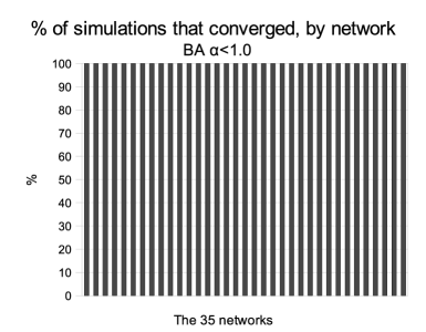
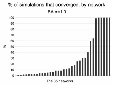
We immediately notice that a higher proportion of simulations reached a fixed point when $\alpha<1$ than when $\alpha=1$. This is not unexpected as the non-determinism in the stochastic trajectories is a way to avoid the cyclic attractors the deterministic trajectories tend to fall into. The remarkable property is that, if for a given network a single trajectory with $\alpha<1$ converged to a fixed point, then all the trajectories with $\alpha<1$ also converged (although not necessarily to the same point). Also note that all the fixed point discovered through fully parallel updates were also discovered with the $\alpha<1$ simulations. This indicates that stochastic updates can be used as a robust method to detect the existence of fixed points.

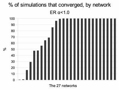
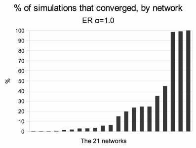
For the Erdös-Rényi networks we computed the same statistics as we did for the scale-free networks, were applicable. There were 27 out of the 50 networks were we found at least a fixed point. Interestingly, only $21$ of those fixed points were detected by deterministic trajectories. The breakdown of percentages of converging trajectories by network for the case $\alpha=1$ is presented in Figure 7. Every single trajectory that did not reach a fixed point ended in a cycle within the time horizon. The breakdown of percentages by network for the case $\alpha<1$ is presented in Figure 7. We notice immediately the difference between Figures 7 and 5: For some Erdös-Rényi networks with fixed point not all stochastic trajectories converged to a fixed point while all trajectories converged in the scale-free networks case, as we already described before.

Figure 6: Percentage of simulations that converged for each of the 27 ER networks where a fixed point was found.

Figure 7: Percentage of simulations that converged for each of the 21 ER networks where a fixed point was found.

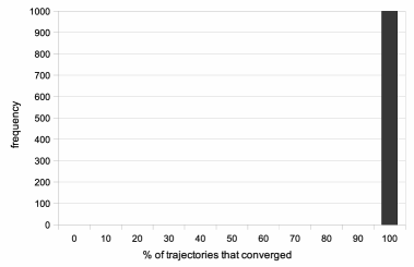
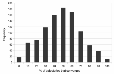
To emphasize the differences in the qualitative behavior we look more closely at two particular networks. We selected one Erdös-Rényi network for which the percentage of trajectories that converged (considering all $\alpha<1$) was about 50%. Recall that 1000 initial configurations were used, 10 values of $\alpha$ were tried and one trajectory per $\alpha$ was simulated. That means that about 5000 out of 10000 trajectories converged to a fixed point for that particular network. The histogram in Figure 9 shows that the choice of the initial configuration changes the probability of reaching a fixed point. The heights of the bars represent numbers of initial configurations. The horizontal axis is the percentage of trajectories (starting from one particular initial configuration) that converged to a fixed point. For instance, for the Erdös-Rényi network, we can deduce the following: 160 initial configurations converged in 40% of the simulations. Since for each initial configuration we ran exactly 10 simulations there is no need to associate intervals with bins. For contrast, we show in Figure 9 the analogous histogram for an arbitrary scale-free network with a fixed point.

Figure 8: Histogram of number of initial configurations that lead to a converging trajectory for a single scale-free network which had at least one fixed point ($\alpha<1$).

Figure 9: Histogram of number of initial configurations that lead to a converging trajectory for a single Erdös-Rényi network which had at least one fixed point ($\alpha<1$).

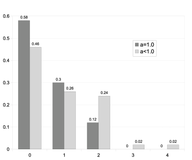
Another difference between the influence of parallelism when updating scale-free or Erdös-Rényi networks is seen comparing Figures 3, 3 and 10. Figure 10 shows the difference in number of fixed points found depending on $\alpha$ being 1 or less than 1. The columns that describe the $\alpha<1$ case represent the same values found in the histogram in Figure 3. The columns that describe the $\alpha=1$ case in Figure 10 show that fewer fixed points were discovered. This, again, strongly suggests that using partially parallel updates is a sensible strategy to find fixed points. It also indicates that the set of discovered fixed points somehow depends on the choice of $\alpha$. For scale-free networks, we also discriminated between $\alpha=1$ and $\alpha<1$ cases. For these networks though, in both cases the histograms were identical to the one in Figure 3. This indicates that the convergence to fixed points is fairly insensitive to the choice of $\alpha$. This property shows a form of robustness of scale-free networks.

Figure 10: Frequency of number of fixed points for ER networks for the $\alpha=1$ and $\alpha<1$ cases.

4.3 Time and work until convergence

For scale-free networks, Figures 12 and 12 represent the mean and maximum time/work to reach the fixed point for only the simulations that reached it. This means, for $\alpha<1$, each column gives the average and maximum over 35000 simulations, while for $\alpha=1$ the values were computed over a smaller sample because only $\sim$28.9% of the runs ended before the time horizon was reached. This makes the values of the rightmost column of each figure somewhat incomparable with the others.

In Figure 12 we note how the average time changes with $\alpha$. The qualitative behavior of the results are in part intuitive. If $\alpha=0$ we expect the time to be high, since not much work is done per iteration. We also expected the time to increase when $\alpha$ approaches 1, because the system becomes more deterministic and tends to imitate the behavior of the $\alpha=1$ case. Therefore, the cycles of the deterministic trajectories become metastable regions of the stochastic trajectories.

Figure 11: Convergence time for scale-free networks

Figure 12: Convergence work for scale-free networks

Figure 13: Filtered convergence time for scale-free networks

Figure 14: Filtered convergence work for scale-free networks

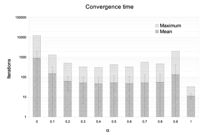
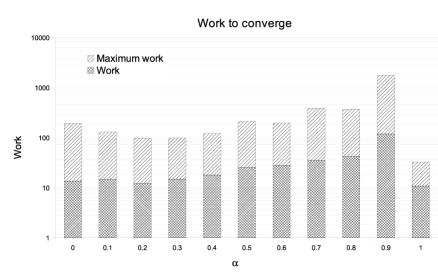
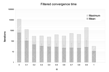
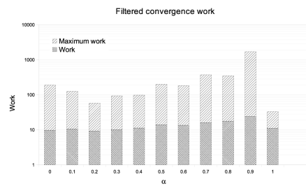
Note that the average number of iterations for $\alpha=1$ is smaller than for all the values for $\alpha<1$. The comparison is not fair, though, because the parallel update rule is not a reliable way to find fixed points. With respect to the amount of work, we can notice, as expected, that small values of $\alpha$ become very competitive (see Figure 12). One possible explanation for the parallel simulations outperforming the $\alpha<1$ cases (neglecting the lack of robustness, of course) is as follows: The $\alpha=1$ updates are prone to solve only the “simple instances” of the problem. That is, only very stable fixed points located close to the initial configurations are likely to be found.

To make a fair comparison between the $\alpha<1$ and $\alpha=1$ situations, we recompute the statistics but only for the cases where the deterministic model found a fixed point. This means, we considered only the pairs (network $G$, initial configuration ${\mathbf{s}}$) such that the deterministic trajectory of $G$ starting from ${\mathbf{s}}$ reached a fixed point. Figures 14 and 14 show the results. From comparison against Figures 12 and 12 we notice that the average times of the simulations for $\alpha<1$ actually decreased. This supports the hypothesis of $\alpha=1$ working mostly for simple instances of the problem. The differences in running time may not be considered substantial though and the problem requires further study.

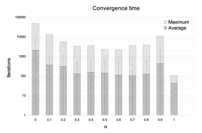
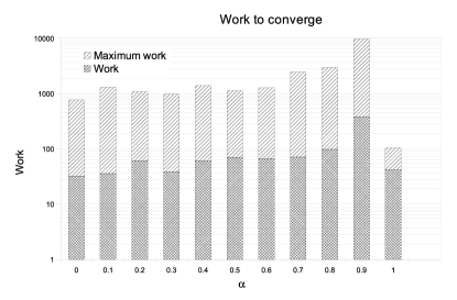
For Erdös-Rényi networks, Figures 16 and 16 are the mean and maximum times/work to reach the fixed point for only the simulations that reached it. This means, for $\alpha<1$, each column gives the average and maximum over 27000 simulations, while for $\alpha=1$ the values were computed over a smaller sample because only $\sim$24% of the runs ended before the time horizon was reached. In this case we did not compute the averages/maximums for the stochastic model restricting the networks and initial conditions to those that reached a fixed point with deterministic updates. There was no qualitative difference between the results for scale-free networks (Figures 12 and 12) and the times for Erdös-Rényi networks. Data suggests that Erdös-Rényi networks are slower to converge than scale-free systems.

Figure 15: Convergence time for Erdös-Rényi networks

Figure 16: Convergence work for Erdös-Rényi networks

4.4 Discussion

We will first make the case that the RBNs, as defined here, have a behavior that resembles that of natural networks. It is well known that gene expression/repression changes according to external cell conditions, such as temperature or availability of nutrients and/or oxygen. For brevity, we will refer to such conditions as EC. This can be modeled easily by setting the values of input nodes depending on the EC. It is also widely accepted that gene expression state is (after the transient) mostly function of the EC. In terms of the model this means the fixed point should be function of the values of the input nodes. Although stochasticity sometimes plays an important role in cell dynamics [25], for purposes of discussion we will assume that for each set of EC there should be one or a small number of fixed points. Another property is stability, meaning the fixed point should have a large basin of attraction. Additionally, the fixed point should be reached “quickly.” By quickly, we mean that the number of transitions should be small compared to the total number of possible configurations. Finally, the behavior of the model should not depend dramatically on the choice of $\alpha$.

Our simulations with asynchronous updates on scale-free networks showed all properties mentioned above. The theorem in Subsection 2.1, together with the histogram in Figure 3 address the number of fixed points is, with high probability, close to one. The fact that all trajectories converged, as shown in Figure 5 shows the model is (robust/stable?) regardless of the choice of $\alpha$, as long as it is less than $1$. With respect to the speed of convergence, the average number of iterations to reach a fixed-point (see Figure) is small compared to the number of possible configurations, which was about $2^{63}$ in all the numerical experiments.

Of course, the goal of the model is to provide insight on biological process. The most remarkable observation is that the three aforementioned properties appeared in the simulations without requiring any kind of deliberate design. The network topologies, the dynamics and vertices to be updates were selected at random. Yet, the behavior was as desired, as long as the network was scale-free and $\alpha<1$. This suggests that the prevalent scale-free topologies in natural GRNs [3] could be a major factor in robustness of living cells.

As an aside, finding fixed points of a Boolean network is equivalent to finding satisfying assignments to Boolean formulas. This is a well known problem in Computer Science, and is believed to be computationally hard if we consider the worst case running time. However, the results shown in Figures 12, 14 and 16, which implies fast convergence, suggest that the asynchronous update rule is an efficient heuristic to find fixed points or satisfying assignments.

5 Conclusions

We analyzed the tendency to reach a fixed point, the number of iterations and the work needed to converge to it for different families of Boolean networks and update policies. We summarize our results as follows:

1. Using partial parallelism (i.e, $\alpha<1$), the likehood of the trajectory to reach a fixed point increases. This happens regardless of topology.

2. For scale-free networks the choice of $\alpha$ is not very important from the convergence point of view, as long as it is less than one. We base this conclusion on the fact that we could not find a simple example of a network not converging to a fixed point provided that it has 1.

3. For scale-free networks the choice of $\alpha$ is not very important from the work point of view, as long as it is less than one. This follows from the analysis of the filtered case. The work is about the same as in the $\alpha=1$ case, while full parallelism increases the likehood of being trapped in a cycle.

4. For Erdös-Rényi networks the choice of $\alpha$ is relevant from the work point of view, when it is less than 1. The set of points discovered seems to be dependent somehow on the choice of $\alpha$.

5. The combination of scale-free networks and using $\alpha<1$ for the updates was enough to impose dynamical properties which are similar to those observed in nature.

6 Acknowledgments

We would like to thank Álvaro Olivera for useful discussion.

References

- [1] R. Albert and A.-L. Barabási. Statistical mechanics of complex networks. Rev. Modern Phys. 74 (1) (2002) 47–97.
- [2] R. Albert and H.G. Othmer. The topology of the regulatory interactions predicts the expression pattern of the segment polarity genes in Drosophila melanogaster. Journal of Theoretical Biology 223 (2003) 1–18.
- [3] R. Albert. Scale-free networks in cell biology. Journal of Cell Science 118 (2005), 4947–4957.
- [4] M. Aldana, S. Coppersmith and L.P. Kadanoff. Boolean dynamics with random couplings. In Perspectives and Problems in Nonlinear Science, Springer Applied Mathematical Sciences Series, Springer, Berlin 2003, 23–89.
- [5] M. Aldana. Boolean dynamics of networks with scale-free topology. Physica D 185 (2003) 45–66.
- [6] E.R. Álvarez-Buylla, Á. Chaos, M. Aldana, M. Bení tez, Y. Cortes-Poza, C. Espinosa-Soto, D.A. Hartasánchez, R.B. Lotto, D. Malkin, G.J. Escalera-Santos and P. Padilla-Longoria. Floral morphogenesis: Stochastic explorations of a gene network epigenetic landscape. PLoS ONE 3(11) (2008): e3626.
- [7] A.-L. Barabási and R. Albert Emergence of scaling in random networks. Science 286 (5439) (1999) 509–512.
- [8] U. Bastolla and G. Parisi. Closing probabilities in the Kauffman model: An annealed computation. Physica D 98, 1–25 (1996).
- [9] H. Bersini and V. Detours. Asynchrony induces stability in cellular automata based models. Proceedings of the Fourth International Workshop on the Synthesis and Simulation of Living Systems: Arti cial Life IV, MIT Press, 1994.
- [10] A. Bhattacharjya and S. Liang. Power-Law distributions in some random Boolean networks. Phys. Rev. Lett. 77, 1644–1647 (1996).
- [11] S. Bilke and F. Sjunnesson. Stability of the Kauffman model. Phys. Rev. E 65 (2001) 016129.
- [12] C. Christensena, A. Gupta, C.D. Maranasand and R Albert. Large-scale inference and graph-theoretical analysis of gene-regulatory networks in B. Subtilis. Physica A (2007) 796–810.
- [13] Ch. Damiani, M. Villani, Ch. Darabos and M. Tomassini. Dynamics of interconnected Boolean networks with scale-free topology. Artificial Life and Evolutionary Computation, proceeding of WIVACE 2008, World Scientific Publication, 27–283.
- [14] Ch. Darabos, M. Tomassini and M. Giacobini. Dynamics of unperturbed and noisy generalized Boolean networks. Journal of Theoretical Biology 260-4, (2009) 531–544.
- [15] E.H. Davidson, J.P. Rast, P. Oliveri, A. Ransick, C. Calestani, C.-H. Yuh, T. Minokawa, G. Amore, V. Hinman, C. Arenas-Mena, O. Otim, C.T. Brown, C. B. Livi, P.Y. Lee, R. Revilla, Al.G. Rust, Z. jun Pan, M.J. Schilstra, P.J.C. Clarke, M.I. Arnone, L. Rowen, R. A. Cameron, D.R. McClay, L. Hood and H. Bolouri. A genomic regulatory network for development. Science 295 (5560) (2002) 1669–1678.
- [16] B. Derrida and Y. Pomeau. Random networks of automata: A simple annealed approximation. Europhysics Letters 1 (2) (1986) 45–49.
- [17] R. Edwards and L. Glass. A calculus for relating the dynamics and structure of complex biological networks. Advances in Chemical Physics, Vol. 132, John Wiley & Sons, New York (2006), 151–178.
- [18] P. Erdös and A. Rényi. On random graphs. Publicationes Mathematicae 6 (1959): 290–297.
- [19] N. Fatès, N. Schabanel, D. Regnault and É. Thierry. Asynchronous behavior of double-quiescent elementary cellular automata. Proceedings of LATIN 2006: 7th Latin American Symposium, LNCS 3887, 2006, 455– 466.
- [20] J. J. Fox and C.C. Hill. From topology to dynamics in biochemical networks. Chaos 11 (4) (2001) 809–815.
- [21] C. Gershenson. Updating schemes in random Boolean networks: Do they really matter? Proceedings of the Ninth International Conference on the Simulation and Synthesis of Living Systems, MIT Press, 2004, 238–243.
- [22] I. Harvey and T. Bossomaier. Time out of joint: Attractors in asynchronous random Boolean networks. Proceedings of the Fourth European Conference on Artificial Life (ECAL97), MIT Press, 199, 67–75.
- [23] S. Huang, G. Eichler, Y. Bar-Yam and D.E. Ingber. Cell fates as high-dimensional attractor states of a complex gene regulatory network. Phys. Rev. Lett. 94: 128701 (2005).
- [24] K. Iguchi, S Kinoshita and H.S. Yamada. Boolean dynamics of Kauffman models with a scale-free network. Journal of Theoretical Biology 247:1, (2007) 138–151.
- [25] M. Kaern, T. C. Elston, W. J. Blake and James J. Collins. Stochasticity in gene expression: from theories to phenotypes, Nature Reviews Genetics 6, 451-464 (June 2005).
- [26] S. Kauffman. Metabolic stability and epigenesis in randomly constructed genetic nets. Journal of Theoretical Biology 22:3 (1969) 437–467.
- [27] B. Mesot and Ch. Teuscher. Critical values in asynchronous random Boolean networks. Advances in Artificial Life, ECAL2003, Vol. 2801 of Lecture Notes in Artificial Life (2003) 367–376.
- [28] C. Oosawa and M.A. Savageau. Effects of alternative connectivity on behavior of randomly constructed Boolean networks. Physica D 170 (2002) 143–161.
- [29] B. Schönfisch and André de Roos. Synchronous and asynchronous updating in cellular automata, Biosystems, Volume 51, Issue 3, 123-143, (September 1999).
- [30] S.H. Strogatz. Exploring complex networks. Nature 410, 268-276 (2001).