The Universal Aspect Ratio of Vortices in Rotating Stratified Flows:
Experiments and Observations

Abstract

We validate a new law for the aspect ratio $\alpha=H/L$ of vortices in a rotating, stratified flow, where $H$ and $L$ are the vertical half-height and horizontal length scale of the vortices. The aspect ratio depends not only on the Coriolis parameter $f$ and buoyancy (or Brunt-Väisälä) frequency $\bar{N}$ of the background flow, but also on the buoyancy frequency $N_{c}$ within the vortex and on the Rossby number $Ro$ of the vortex such that $\alpha=f\,[Ro\,(1+Ro)/(N_{c}^{2}-\bar{N}^{2})]^{1/2}$. This law for $\alpha$ is obeyed precisely by the exact equilibrium solution of the inviscid Boussinesq equations that we show to be a useful model of our laboratory vortices. The law is valid for both cyclones and anticyclones. Our anticyclones are generated by injecting fluid into a rotating tank filled with linearly-stratified salt water. The vortices are far from the top and bottom boundaries of the tank, so there is no Ekman circulation. In one set of experiments, the vortices viscously decay, but as they do, they continue to obey our law for $\alpha$, which decreases over time. In a second set of experiments, the vortices are sustained by a slow continuous injection after they form, so they evolve more slowly and have larger $|Ro|$, but they also obey our law for $\alpha$. The law for $\alpha$ is not only validated by our experiments, but is also shown to be consistent with observations of the aspect ratios of Atlantic meddies and Jupiter’s Great Red Spot and Oval BA. The relationship for $\alpha$ is derived and examined numerically in a companion paper by Hassanzadeh et al. (2012).

1 Introduction: vortices in stratified rotating flows

The Great Red Spot and other large vortices such as the Oval BA Marcus (1993) are persistent giant anticyclonic vortices in Jupiter’s atmosphere. Their vertical aspect ratios $\alpha=H/L$ lie in the range $0.03\leq\alpha\leq 0.1$. In the Atlantic Ocean, meddies are also long-lived anticyclones made of water of Mediterranean origin that is warmer and saltier than the ambient Atlantic. Their lifetimes can be as long as several years, and they have $\alpha\simeq 0.01$ (with $H\simeq 0.5$ km and $L\simeq 50$ km). Presumably, the aspect ratios of these vortices are the result of a competition between rotation and stratification. A rapidly rotating flow, parameterized by a large Coriolis parameter $f$ and small characteristic azimuthal velocity ${V}_{\theta}$ (i.e., small Rossby number $Ro={V}_{\theta}/fL$) is controlled by the Taylor-Proudman theorem: flows have little variation along the rotation axis and form columnar vortices with large $\alpha$. In contrast, strongly stratified flows, parameterized by large buoyancy frequencies

$$N\equiv\sqrt{-\frac{g}{\rho}\frac{d\rho}{dz}}$$ (1)

inhibit vertical motions and form baroclinic vortices, often appearing as thin “pancake” vortices Billant & Chomaz (2001). Here $\rho$ is the fluid density, $g$ is gravity, $z$ is the vertical coordinate.

The goal of this paper is to investigate this competition and determine and verify a quantitative law for $\alpha$. Previous experimental studies that used constant-density fluids to simulate meddies or Jovian vortices (Sommeria et al., 1988; Antipov et al., 1986) prohibited this competition and resulted in laboratory vortices that were barotropic Taylor columns that extended from the bottom to the top of the tank. Thus, $\alpha$ was imposed by the boundaries of the tank. In our experiments, the vortices are created near the center of a large tank so that the tank’s boundaries have no or little influence on $\alpha$, and there is little or no Ekman circulation in the tank and no Ekman spin-down of our vortices.

2 Aspect ratio law of a model vortex

The dissipationless, Boussinesq equations for a fluid with mean density $\rho_{0}$ in the rotating frame (and ignoring the centrifugal force) are

$${{\partial{\bf v}}\over{\partial t}}=-({\bf v}\cdot\nabla){\bf v}-{{\nabla p}\over{\rho_{0}}}+f{\bf v}\times\hat{\bf z}-{{(\rho-\rho_{0})}\over{\rho_{0}}}g\,\,\hat{\bf z}\,\,\,\,\textrm{and}\,\,\,\,{{\partial\rho}\over{\partial t}}=-({\bf v}\cdot\nabla)(\rho-\bar{\rho})+v_{z}\,\rho_{0}\,\frac{\bar{N}^{2}}{g}$$ (2)

where ${\bf v}$ is the divergence-free velocity, $v_{z}$ the vertical component of the velocity, $p$ is the pressure, $z$ is vertical coordinate, $\hat{\bf z}$ is a unit vector, and an overbar above a quantity indicates that the quantity is the equilibrium value in the undisturbed, linearly-stratified (i.e., with constant $\bar{N}$) fluid. The unperturbed solution has $\bar{{\bf v}}=0$; $\bar{\rho}=-(\bar{N}^{2}/g)\rho_{0}\,z+\rho_{0}$; and $\bar{p}=(\bar{N}^{2}\rho_{0}/2)\,z^{2}-g\,\rho_{0}\,z+p_{0}$, where $p_{0}$ is an arbitrary constant. One steady solution of the Boussinesq equations that consists of an isolated, compact vortex with solid body rotation $\Omega$ has ${\bf v}\equiv\bar{{\bf v}}=0$; $\rho\equiv\bar{\rho}$; and $p\equiv\bar{p}$ everywhere outside the vortex boundary; while inside the vortex: $v_{\theta}=\Omega\,r$; $v_{z}=v_{r}=0$; $\rho=-({N_{c}}^{2}/g)\,\rho_{0}\,z+\rho_{0}$; and ${p}=({N_{c}}^{2}\,\rho_{0}/2)\,z^{2}-g\,\rho_{0}\,z+[\Omega\,(\Omega+f)\,\rho_{0}/2]\,r^{2}+p_{c}$, where $r$ is the cylindrical radial coordinate, $v_{r}$ and $v_{\theta}$ are the radial and azimuthal components of the velocity; $p_{c}$ is a constant equal to $p_{0}-\rho_{0}\,\Omega\,(\Omega+f)\,L^{2}/2$, and $L$ is the radius of the vortex at $z=0$. This vortex has a uniform buoyancy frequency $N_{c}$ throughout the entire vortex (in general, the subscript $c$ means the quantity is to be evaluated at the vortex center, i.e., at $r=0$ and $z=0$). The vortex boundary is determined by requiring that the pressure be continuous throughout the flow. But note that the density and velocity are discontinuous at the vortex boundary). Continuity of $p$ requires the vortex boundary to be ellipsoidal:

$$(r/L)^{2}+(z/H)^{2}=1,$$ (3)

where the semi-height is $H\equiv\sqrt{2\,(p_{0}-p_{c})/[\rho_{0}\,({N_{c}}^{2}-\bar{N}^{2})]}$, and the semi-diameter is $L\equiv\sqrt{2\,(p_{0}-p_{c})/[\Omega\,\rho_{0}\,(f+\Omega)]}$. This vortex has aspect ratio

$$\alpha\equiv H/L=\left(\frac{Ro\,(1+Ro)}{{N_{c}}^{2}-\bar{N}^{2}}\right)^{1/2}f,$$ (4)

where the Rossby number $Ro\equiv\omega_{c}/2f=\Omega/f$. We have defined $Ro$ in terms of the vertical vorticity $\omega$ at the vortex center to make our expression in equation (4) consistent with a more general relationship for $\alpha$ that is derived in the companion paper of Hassanzadeh et al. (2012) by assuming that the vortex has cyclo-geostrophic balance in the horizontal directions and hydrostatic balance in the vertical direction. For cyclones: $Ro>0$, $p_{0}>p_{c}$ and $N_{c}>\bar{N}$. For cyclostrophic anticyclones: $Ro<-1$, $p_{0}>p_{c}$, and $N_{c}>\bar{N}$, but for quasi-geostrophic anticyclones: $-1<Ro<0$, $p_{0}<p_{c}$, and $N_{c}<\bar{N}$.

3 Comparison with previous observations or predictions of vortex aspect ratio $\alpha$

Our law (4) for the aspect ratio $\alpha$ agrees with previous experiments in rotating and stratified flows. For example, Bush & Woods (1999) created vortices in a rotating stratified fluid from the break-up of small-diameter rising plumes. Very little ambient fluid becomes entrained in a rising plume or when the plume breaks and rolls up into vortices, so the vortex cores have nearly uniform density, so $N_{c}=0$. Due to angular momentum conservation, the vorticity within plumes rising from a small diameter orifice have no angular momentum or angular velocity when viewed in the inertial frame. When viewed in the rotating frame with angular velocity $f/2$, these plumes have an angular velocity $\Omega=-f/2$. Thus, in the rotating frame these vortices are anticyclones with $Ro\simeq-0.5$. With parameter values $N_{c}=0$ and $Ro=-0.5$, equation (4) predicts $\alpha=0.5f/\bar{N}$, which agrees well with the experiments of Bush & Woods (1999) that found $\alpha=0.47f/\bar{N}$.

It is often claimed that quasi-geostrophic (QG) vortices obey the scaling law $H/L=f/\bar{N}$ Reinaud et al. (2003); Dritschel et al. (1999); McWilliams (1985), independently of the values of $Ro$ and $N_{c}$. This scaling is broadly used among the oceanographic community for vortices created from noise but is sometimes applied to Atlantic meddies and other vortices without close neighbors. We show in sections 4 and 5 that the aspect ratios of our experimental vortices and meddies have shapes that strongly depend on $Ro$ and their internal stratifications $N_{c}$, and therefore $\alpha\neq f/\bar{N}$ for these vortices.

In a theoretical inviscid analysis, Gill (1981) proposed that $\alpha$ should be proportional to $Ro\,(f/\bar{N})$. In this study, the velocity and the density fields were searched as continuous solutions of the thermal wind equation in 2D. A direct consequence of this constraint (that we avoid in our analysis as discontinuous fields are solutions of the primary non viscous equations) is that the scales of the vortices are in fact imposed by the shape of the solutions that match the fields inside and outside the vortices. These scales are not the characteristic lengths of a real discontinuous patch of vorticity and density anomaly as defined in section 2. Note that in reality, viscosity will smooth the discontinuity of the patch, but this process will not influence the aspect ratio of the vortex. Moreover, as shown in the companion paper of Hassanzadeh et al. (2012), Gill’s law is only valid for the outer field contrary to his solution for the inner field that satisfies our law (4) in the geostrophic limit. Therefore, we think that Hedstrom & Armi (1988) experimentally checked the law derived by Gill (1981) for the outer field only. It appears that in this experimental work, the measurements were made while the vortices were very young, still undergoing geostrophic adjustment and far from equilibrium. As described below, by performing similar experiments but waiting until the vortices come to a quasi-static equilibrium, the aspect ratio of the vortices indeed obeys equation (4).

Note finally that our scaling law, modified for use with discrete layers of fluid rather than a continuous stratification, also applies to the models of anticyclonic ocean eddies used by Nof (1981) and by Carton (2001).

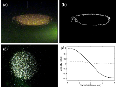
Figure 1: Aspect ratio and Rossby number. Upper panels: Determination of the aspect ratio $\alpha=H/L$. (a) Side view of laboratory anticyclone with $\bar{N}=2.3$ rad/s and $f=2$ rad/s. (b) Image processing of vortex in panel (a) to determine $\alpha$. Here $\alpha=0.3$ with $H=1.9$ cm and $L=6.3$ cm. Lower panels: Determination of $Ro$. (c) Top view of laboratory anticyclone with $\bar{N}=2$ rad/s, $f=2$ rad/s, and $Ro=-0.13$. (d) Azimuthal $v_{\theta}$ ($-$) and radial $v_{r}$ ($--$) velocities of flow in panel (c) as functions of radius $r$. The core has a solid body-like rotation. The magnitude of $v_{r}$ is consistent with the R.M.S. fractional uncertainty of $v_{\theta}$, which is $\pm 5$–10%. The fractional uncertainties in $\bar{N}$ are $\pm 10$%.

4 Application to Laboratory Vortices

We have carried out a study of vortices in a rotating, stratified laboratory flow in a transparent tank of dimensions $50\times 50\times 70$ cm³ mounted on a rotating table. Using the classic double-bucket method with salt water Oster (1965), each experiment initially has a linear vertical stratification, with a constant buoyancy frequency $\bar{N}$ independent of location. The values of $\bar{N}$ in our experiments varied from $1$ rad/s to $2.3$ rad/s. The Coriolis parameter $f$ can be as large as $7$ rad/s. Two sets of experiments have been carried out following respectively seminal works by Griffiths & Linden (1981) and Hedstrom & Armi (1988). In the first one, once the fluid in the tank reaches solid-body rotation, we briefly inject a small volume of fluid with constant density $\rho_{0}$ through a $3$ mm diameter pipe along the axis of rotation at depth approximately midway between the top and bottom of the tank. As soon as the fluid is injected, it is deflected horizontally by the stratification and the Coriolis force organizes it into a freely decaying anticyclone. In a second set of experiments, the vortex is permanently sustained by a smooth and stationary injection, using a peristaltic pump whose flux rate is chosen between $6$ and $500$ mL/min, through the $3$ mm diameter pipe with a piece of porous material fixed at the end of the pipe. The technique in the second second set of experiments allows us to create vortices with higher Rossby numbers than in the first set. Moreover the sustained anticyclones in the second set of experiments evolve very slowly compared with those in the first set. In both sets of experiments, the injected fluid is seeded with fluorescein dye and $100$ $\mu$m–diameter particles for Particle Image Velocimetry (PIV) Meunier & Leweke (2003). We follow the evolution of the vortices using one horizontally and one vertically illuminated laser sheet. Video images of the vertical cross-section allow us to record the changes in time of the vortex aspect ratio (figure 1(a) and (b)), while the PIV measurements in the horizontal sheet allow us to find the azimuthal and radial components of the velocity of the vortex, which lead to the determination of $Ro$ (figure 1(c) and (d)).

4.1 Freely decaying vortices

The brief injection of fluid with density $\rho_{0}$ at height $z$ (where $\bar{\rho}(z)=\rho_{0}$) is immediately followed by fast adjustments where the injected fluid becomes approximately axisymmetric. After axisymmetrization, $|V_{\theta}|$ and $|Ro|$ decay very slowly in time with the vortices persisting for $1000$ to $1800$ table rotation times ($4\pi/f$), or several hundred turnaround times of the vortices ($2\pi/(fRo)$). The vortex persists as long as the density anomaly $(\rho-\bar{\rho})$ does. During the slow decay, the vortex core passes through a series of quasi-equilibrium states where it has approximately solid-body rotation with negligible radial velocity as shown on figure 1(d). The experimentally measured boundaries of one of the slowly-decaying anticyclones that were created by injection are shown at four different times in figure 2. Also shown are the boundaries of our theoretical model of the decaying vortex. Our model is the solid-body rotating vortex with a discontinuous velocity derived in section 2 with $N_{c}\equiv 0$ and with the ellipsoidally-shaped boundary given by equation (3). Due to the slow diffusion of salt, we assume that for all time the fluid density within the model vortex remains at its initial value of $\rho_{0}$, so we assume that $N_{c}=0$ for all time. Due to the lack of diffusion in the laboratory vortex, we also assume that within the ellipsoidal boundary of the model vortex, the volume $4/3\pi H(t)L(t)^{2}=4/3\pi\alpha(t)L(t)^{3}$ remains constant, despite the fact that $\alpha$ and $L$ change in time. The theoretical boundaries of our model vortices are computed with equation (3), where $\alpha(t)$ is given by our law (4), where $Ro(t)$ is measured experimentally, $N_{c}$ is assumed to be zero, $f$ is known, $\bar{N}$ is assumed to remain at its initial value, and where $L(t)$ is computed by assuming that the volume of the ellipsoid is constant in time. That is, we set

$$L(t)=L_{0}\,[\alpha_{0}/\alpha(t)]^{1/3}$$ (5)

where the value of $L_{0}$ is the experimental value of $L$ from the first panel with $Ro=-0.08$; $\alpha_{0}$ is the initial value of $\alpha$ found from equation (4) with $Ro=-0.08$ and $\alpha(t)$ is determined from $Ro(t)$ using equation (4).

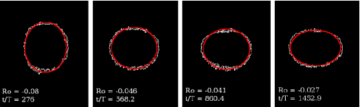
Figure 2: Image-processed side-view of a vortex boundary (white) at different times $t$ with $f=6.8$ rad/s and $\bar{N}=1.6$ rad/s held fixed. $|Ro|$ decreases in time. Also shown are the theoretical boundaries (gray in print; red online) of the model vortices at each time. The model vortex has $H/L$ given by equation (4), so the coincidence of the gray (or red) and white curves validates our law. $T=4\pi/f$ is the period of the rotating turntable. Because $f/\bar{N}=4.25$ is the same for all of these vortices, while $\alpha$ differs, it is clear that the scaling law $\alpha=f/\bar{N}$ is not correct for these vortices.

Figure 2 shows that the boundaries of the laboratory and model vortices are nearly coincident at four different times, and at those times the vortices have four different Rossby numbers and four different aspect ratios. This validates the law (4) for $\alpha$ and also shows that our assumptions that $N_{c}=0$ and that the volume of the vortex remains constant are both good. If the correct scaling law were $H/L=f/\bar{N}$, rather than law (4), then the vortex in figure 2 would have the same aspect ratio through time, which it clearly does not. Using the scaling law of Gill (1981) with a $Ro$ dependence would lead to a smaller predicted aspect ratio by a factor between $3.4$ and $6$.

4.2 Vortices sustained by continuous injection

In a second set of experiments, the vortices are sustained by a continuous injection of fluid with density $\rho_{0}$ at a fixed flux rate, as in experiments of Griffiths & Linden (1981). The characteristic values of the $Ro$ of these vortices range between $-0.45$ and $-0.20$. With continuous injection the volume of these vortices slowly increases in time and the Rossby number of the vortices decays very slowly compared to the viscously decaying vortices discussed in section 4.1. The continuous injection is laminar and the rate of injection is sufficiently small so that the volume of the vortices increases by only approximately $1\%$ per table rotation. As a consequence, we use the same theoretical, elliptical model for these vortices as we used for the viscously dissipating vortices analyzed in section 2. The experimentally measured boundaries at four different times of a vortex sustained with continuous injection are shown in figure 3. As before, the aspect ratio of the extracted shape of the laboratory vortex is compared to the $\alpha$ of our model vortex that uses law (4) with $N_{c}=0$, the observed value of $Ro$, for $\alpha$, and the volume calculated with the flux rate of the experiment and time $t/T$. As can be seen, the comparison is excellent and validates our theoretical law (4) in the cyclo-geostrophic regime.

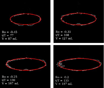
Figure 3: Image-processed side-view boundaries of a vortex sustained with continuous injection at different times. The flow has $f=1.62$ rad/s, $\bar{N}=2.3$ rad/s, and an injection rate of $10$ mL/min. Also shown are the theoretical boundaries of the model vortices. Line colors are as in figure 2. The model vortex has $H/L$ given by equation (4), so the coincidence of the boundaries of the laboratory and model vortex validates equation (4) for $\alpha$. Unlike the vortex in figure 2, the vortex volume $V$ changes in time. $Ro$, $V$, and time $t$ are given for each image.

Note that in the similar experiments of Griffiths & Linden (1981) briefly described in section 5 of their article, continuous intrusions of fluid into density gradients were performed. They observed vortices with aspect ratios of $0.47$ and $0.99$. In these two experimental runs, $\bar{N}H/fL$ was estimated around $0.3$, which is in disagreement with Charney’s QG law. As no precise measurement of the Rossby number was done, no comparison is possible with either our law or Gill’s theory Gill (1981).

5 Application to Meddies and Jovian Vortices

Our law (4) for vortex aspect ratio $\alpha$ also applies to ocean meddies, which, unlike our laboratory vortices, are internally stratified (i.e. $N_{c}\neq 0$). Using the reported values of the ocean densities as functions of position within and outside the meddies Armi et al. (1988); Hebert et al. (1990); Pingree & Le Cann (1993); Tychensky & Carton (1998), we have compiled in table 1 average values of the buoyancy frequencies of the meddies ${N}_{c}$ and their background environments $\bar{N}$, along with the observed values of $\alpha$, $L$ and $Ro$. Note that according to our law (4), the effects of non-zero $N_{c}$ do matter on the aspect ratio, especially when $N_{c}$ is of order $\bar{N}$, as it is for the meddies (and Jovian vortices – see below), has a large effect on the aspect ratio. For all but the oldest meddy shown in figure 4, law (4) fits the observations. Note that setting $\alpha$ equals to the alternative scaling $f/\bar{N}$ does not fit the meddy data, even with the large uncertainties of the observed values of $\alpha$ of the meddies shown in figure 4. Setting $\alpha$ equals to the other alternative scaling discussed in section 3, $Ro\,(f/\bar{N})$ Gill (1981); Hedstrom & Armi (1988), is an even poorer fit.

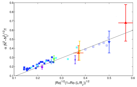
Figure 4: Tests of our theoretical law (4) (straight line) for $\alpha$. The theory agrees with our freely decaying vortex experiments ($\blacksquare$) with $1.6$ rad/s $\leq f\leq 7~{}$rad/s and with our sustained vortex experiments with $f=1.6$ rad/s and $N=2.3$ rad/s ($\square$); with Bush & Woods’ experiments at $Ro=-0.5$ (Bush & Woods, 1999) ($\blacktriangledown$); with Jupiter’s Great Red Spot and Oval BA Marcus (1993); Shetty & Marcus (2010); de Pater et al. (2010)($\blacktriangle$); and with meddies Sharon Armi et al. (1988); Hebert et al. (1990); Schlutz Tokos & Rossby (1990)($\times$), Bobby Pingree & Le Cann (1993)($\star$), Hyperion ($\circ$), Ceres ($\bullet$) and Encelade ($\diamond$) Tychensky & Carton (1998). All the data for the meddies are given in table 1. Data and error bars for the Jovian vortices are discussed in the online supplementary material. Error bars for the meddies are dominated by uncertainties in $(\bar{N}^{2}-N_{c}^{2})$, which are due to uncertainties in the reported densities and temperatures of meddies. Meddy Sharon is the oldest meddy shown, so dissipation could have modified its shape.

Law (4) also applies to Jovian vortices. For the Great Red Spot (GRS) it is necessary to take into account the fact that the characteristic horizontal length $L$ of the derivative of the pressure anomaly $(p-\bar{p})$ is nearly 3 times smaller than the characteristic radius $R_{v}$ where the azimuthal velocity reaches its peak value Shetty & Marcus (2010). As shown in our companion paper by Hassanzadeh et al. (2012), when $R_{v}\gg L$, the scaling law should be modified so that the numerator $Ro\,(1+Ro)$ in equation (4) is replaced with $Ro\,[1+Ro\,(L/R_{v})]$. With the exceptions of $H$ and $N_{c}$, the properties of Jovian vortices are well known and have small uncertainties Shetty & Marcus (2010). Based on observations of the haze layers above the GRS and Oval BA, most observers agree that the elevations of their top boundaries Banfield et al. (1988); Fletcher et al. (2010); de Pater et al. (2010) are near the elevation of 140 mb pressure. There is less agreement on the elevations of the mid-plane ($z=0$) of the vortices. Some modelers Morales-Juberias et al. (2003) of the Oval BA, set $z=0$ to be 680 mb (the height of the clouds from which the velocities are extracted), making $H=34$ km. However, some observers de Pater et al. (2010) argue that $z=0$ is deeper at 2000 mb, making $H=$ 59 km. Other modelers Cho et al. (2001) choose $H$ of the GRS to be approximately one pressure scale height ($23$ km). Based on these observations and arguments, we set the “observed” value of $H$ to be $45\pm 13$ km.

Jovian values of $\bar{N}$ have been measured accurately Shetty & Marcus (2010), and as shown in the online supplementary material, the values of $(\bar{N}^{2}-N_{c}^{2})$ and their uncertainties for the GRS and the Oval BA can be inferred from thermal imaging, which provides the temperatures of the vortices and of the background atmosphere. We show in the online supplementary material how the values and uncertainties of $N_{c}$ for the GRS and Oval BA that are used in table 1 are calculated from the observed temperature measurements and also how the values of $Ro$ for the Jovian vortices in table 1 were calculated. Using the values in table 1 for the properties of the Jovian vortices and of the background Jovian atmosphere we have included the aspect ratio information of the GRS and Oval BA in figure 4. The figure shows that the aspect ratios of the Jovian anticyclones are consistent with our law (4) for $\alpha$ (with the correction due to fact that $R_{v}\neq L$ for the GRS). Even with the large uncertainties in $H$, the data show that the aspect ratios of the Jovian vortices are not equal to $f/\bar{N}$ or to $Ro\,\,(f/\bar{N})$.

Data	$\sqrt{{\bar{N}}^{2}-{N_{c}}^{2}}$	$N_{c}$	$f$	$Ro$	$Observed$	$L$
	(rad/s)	(rad/s)	(rad/s)		$\alpha$	(km)
Experiment 1	$1.6$	$0$	$6.8$	$-0.32$ - $-0.02$	$1.71$ - $0.68$	-
Experiment 2	$1.6$	$0$	$3.2$	$-0.16$ - $-0.03$	$0.82$ - $0.38$	-
Experiment 3	$2.3$	$0$	$1.6$	$-0.45$ - $-0.2$	$0.36$ - $0.27$	-
Bush & Wood’s exp.	$0.78$ - $1.4$	$0$	$0.4$ - $2.2$	$-0.5$	$0.13$ - $1.32$	-
Meddy Ceres	$0.0022$	$0.002$	$8.46\,10^{-5}$	$-0.05$	$0.0073$	$35$
Meddy Hyperion	$0.0024$	$0.0018$	$8.46\,10^{-5}$	$-0.07$	$0.009$	$45$
Meddy Encelade	$0.0026$	$0.0015$	$8.1\,10^{-5}$	$-0.08$	$0.009$	$45$
Meddy Sharon	$0.0021$	$0.0011$	$7.7\,10^{-5}$	$-0.15$	$0.01$	$32$
Meddy Bobby	$0.0015$	$0.0017$	$8.3\,10^{-5}$	$-0.17$	$0.018$	$27$
Jupiter’s Oval BA	$0.0048$	0.018	$1.92\,10^{-4}$	$-0.16$	$0.014$	$3200$
Jupiter’s GRS	$0.0047$	0.015	$1.37\,10^{-4}$	$-0.38$	$0.020$	$2300$
						($R_{V}$=$6260$ km)

Table 1: Data for figure 3. The three sets of laboratory experiments listed in the top three lines have different values of $\bar{N}$ and $f$. Experiment 1 and 2 correspond to a freely decaying vortex and experiment 3 to a sustained vortex. Each set of experiments had vortices with different values of $Ro$, but in all of our laboratory experiments, we assumed $N_{c}=0$ and that $R_{v}=L$. $2L$ and $2H$ were defined to be the horizontal and vertical diameters of the vortices as determined by our edge-finding algorithm (c.f. figure 2). The uncertainties in the laboratory measurements are dominated by the small non-axisymmetric component of the vortices. The fractional uncertainties in $\bar{N}$ are $\pm 10$%. For the meddies, the values of $\bar{N}$ and $N_{c}$ are such that $1.33<\bar{N}/N_{c}<2.16$. The parameter values and their uncertainties for the Jovian vortices are discussed in section 5 and in the online supplementary material. Note that the Jovian values of $\bar{N}$, $f$ and $L$ are known with small uncertainties but that $H$ has large uncertainties.

6 Conclusions

We have derived and verified a new law (4) for the aspect ratio $\alpha\equiv H/L$ of vortices in stratified, rotating flows; the law depends on the Coriolis parameter $f$, the Rossby number $Ro$, the stratification of the ambient fluid $\bar{N}$, and also on the stratification inside the vortex $N_{c}$. This law derived in a more general context in the companion paper of Hassanzadeh et al. (2012) fits exactly the equilibrium solution of the Boussinesq equations that we used to model our laboratory anticyclones. We have shown that the law works well for predicting the aspect ratios of freely decaying anticyclones in the laboratory, of laboratory vortices that are sustained by continuous fluid injection, of Jovian vortices, and of Atlantic meddies. These vortices span a large range of Rossby numbers, occur in different fluids, have different ambient shears, Reynolds numbers and lifetimes, and are created and dissipated by different mechanisms. For these vortices we have demonstrated that a previously proposed scaling law, $H/L=f/\bar{N}$, is not correct. Our law (4) for $\alpha$ shows that equilibrium cyclones must have $\bar{N}<N_{c}$, that anticyclones with $|Ro|<1$ have $\bar{N}>N_{c}$ and that anticyclones with $|Ro|>1$ have $\bar{N}<N_{c}$. Mixing within a vortex tends to de-stratify the fluid inside of it and therefore naturally decreases $N_{c}$ from its initial value. Therefore, if there is mixing and if there is no active process that continuously re-stratifies the fluid within a vortex, then at late times one would expect that $N_{c}<\bar{N}$, and then according to our law only anticyclones with $Ro<1$ can be in equilibrium. This may explain why there are more anticyclonic than cyclonic eddies in the ocean, and also why there appear to be more long-lived anticyclones than cyclones on Jupiter, Saturn and Neptune.

Acknowledgements: We thank the France Berkeley Fund, Ecole Centrale Marseille, and the Russell Severance Springer Professorship endowment that permitted this collaborative work. We also acknowledge financial support from the Planetology National Program (INSU, CNRS).

Online Supplementary Material

7 Properties of the Jovian atmosphere and vortices

To compute the values of the GRS and the Oval BA shown in table 1, we used $g=25$ m s^-2 and $H=45\pm 13$ km. For the GRS de Pater et al. (2010); Shetty & Marcus (2010) we used $\bar{N}=0.0158\pm 0.0005$ rad/s, $V_{\theta}=119\pm 14$ m/s, $L=2300\pm 70$ km, $R_{v}=6260\pm 50$ km, and $f=1.374\times 10^{-4}$ rad/s. For the Oval BA we used $\bar{N}=0.0182\pm 0.0006$ rad/s, $V_{\theta}=101\pm 9$ m/s, $L=3200\pm 45$ km, $R_{v}=3200\pm 45$ km, and $f=1.915\times 10^{-4}$ rad/s de Pater et al. (2010); Shetty & Marcus (2010).

Thermal imaging of the Jovian atmosphere gives the values of the temperature of the clouds at the elevations of the Great Red Spot (GRS) and Oval BA. In particular, the imaging gives the temperature $T_{c^{\prime}}$ (where $c^{\prime}$ indicates the intersection of the vertical central rotation axis of a vortex and the the top of the vortex at $z=H$). Thermal imaging also gives the value of the background temperature $\bar{T}|_{z=H}$ of the atmosphere at the elevation of the top of the vortex and at the latitude of the principal east-west axis of the vortex. For a vortex that is in cyclo-geostrophic equilibrium, at all elevations $z$, the Coriolis and centrifugal accelerations due to the azimuthal velocity of the vortex are balanced by the horizontal pressure gradient within the vortex (Hassanzadeh et al., 2012). The top of the vortex, $z\equiv H$, is defined to be the location where the azimuthal velocity of the vortex is zero. Therefore at $z=H$, the horizontal pressure gradient within the vortex is zero. Therefore, in an ideal gas at the top of a vortex, $[T_{c^{\prime}}-(\bar{T}|_{z=H})]/(\bar{T}|_{z=H})=-[\rho_{c^{\prime}}-(\bar{\rho}|_{z=H})]/(\bar{\rho}|_{z=H})\simeq-H[(\partial\rho/\partial z)|_{c^{\prime}}-(\partial\bar{\rho}/\partial z)]/(\bar{\rho}|_{z=H})\simeq(H/g)(N_{c}^{2}-\bar{N}^{2})$, where the first approximate equality in this expression comes from using the first term in a Taylor series expansion to compute the density difference, and the second approximate equality comes from the definitions of the buoyancy frequencies. Thus, we can set the value of $(N_{c}^{2}-\bar{N}^{2})$ for the Jovian vortices equal to the observed value of ${{g[T_{c^{\prime}}-(\bar{T}|_{z=H})]}\over{H(\bar{T}|_{z=H})}}$.

Following Morales-Juberias et al. (2003), we set the upper elevation of the GRS to be at 140 mbar and use temperature measurements at that elevation. Satellite observations of the GRS (see figure 8 of Fletcher et al., 2010) give $[T_{c^{\prime}}-(\bar{T}|_{z=H})]/(\bar{T}|_{z=H})=-0.041\pm 0.015$. Our estimate of the uncertainty of the Jovian temperatures of the GRS are based on the standard deviation of the data in the top-right panel of figure 8 in Fletcher et al. (2010). The values of $\sqrt{{\bar{N}}^{2}-{N_{c}}^{2}}$ and $N_{c}$ in table 1 for the GRS are based on these temperatures and uncertainties.

There have been no direct measurements of the temperature difference across the top of the Oval BA, but there were thermal measurements of the three White Oval vortices that existed at the same latitude as the Oval BA before it formed (and from which it formed). We use these White Ovals as a proxy for the Oval BA because it has been argued de Pater et al. (2010) that the White Ovals were dynamically similar to the Oval BA and also of the same size and shape. For the Ovals, $[T_{c^{\prime}}-(\bar{T}|_{z=H})]/(\bar{T}|_{z=H})=-0.04\pm 0.015$. For the Oval BA, we used the temperatures from figure 1 of Conrath et al. (1981). The uncertainty of those temperature measurements was not published, so our estimate of the uncertainty is based on the standard deviation of the values of $[T_{c^{\prime}}-(\bar{T}|_{z=H})]$ of the three White Ovals at $140$ mbar. The values of $\sqrt{{\bar{N}}^{2}-{N_{c}}^{2}}$ and $N_{c}$ in table 1 for the Oval BA are based on these temperatures and uncertainties.

To apply our equation (4) correctly to the Jovian vortices, which are not axisymmetric because they are embedded in strongly shearing east-west winds, it is necessary to consider the derivation of the equation for $\alpha$ based on cyclo-geostrophic balance shown in the companion paper (Hassanzadeh et al., 2012). The law for $\alpha$ can be obtained from the vertical hydrostatic equilibrium and cyclo-geostrophic balance applied to the east-west component of the force along the principal east-west axis of the vortex. The shearing east-west wind does not enter into this balance and therefore the Rossby number $Ro=V_{\theta}L/f$ that comes from this derivation and that appears in equation (4) for $\alpha$ (and that is reported in table 1), is based on the values of the north-south velocities along the east-west principal axis. Similarly the value of $L$ that should be used in $Ro$ (and that is reported in table 1) is that of the characteristic length scale of the pressure gradient along the east-west principal axis. Consistent with our approach of deriving the relationship for $\alpha$ by balancing the east-west component of the forces along the east-west principal axis, the measurements of $[T_{c^{\prime}}-(\bar{T}|_{z=H})]$ that should be used in approximating $(N_{c}^{2}-\bar{N}^{2})$ of the Jovian vortices were made along the vortex’s east-west principal axis.

References

- Antipov et al. (1986) Antipov, S. V., Nezlin, M. V., Snezhkin, E. N. & Trubinikov, A. S. 1986 Rossby autosoliton and stationary model of the Jovian Great Red Spot. Nature 323, 238–240.
- Armi et al. (1988) Armi, L. et al. 1988 The history and decay of a Mediterranean salt lens. Nature 333, 649–651.
- Banfield et al. (1988) Banfield, D., Gierasch, P.J., Bell, M., Ustinov, E., Ingersoll, A. P., Vasada, A. R., West, R. A. & Belton, M. J. S. 1988 Jupiter’s cloud structure from Galileo imaging data. Icarus 135, 230–250.
- Billant & Chomaz (2001) Billant, P. & Chomaz, J-M. 2001 Self-similarity of strongly stratified inviscid flows. Phys. Fluids 13, 1645–1651.
- Bush & Woods (1999) Bush, J. M. W. & Woods, A.W. 1999 Vortex generation by line plumes in a rotating stratified fluid. J. Fluid Mech. 388, 289–313.
- Carton (2001) Carton, X. 2001 Hydrodynamical Modeling of Oceanic Vortices. Surveys in Geophysics 22, 179–263.
- Cho et al. (2001) Cho, J. Y.-K., de la Torre Juarez, M., Ingersoll, A. P. & Dritschel, D. G. 2001 A high resolution, three-dimensional model of Jupiter’s Great Red Spot. J. Geophys. Res. 106, 5099–5105.
- Conrath et al. (1981) Conrath, B. J., Flassar, F.M., Pirraglia, J. A., Gierash, P. J. & Hunt, G.E. 1981 Thermal structure and dynamics of the Jovian atmosphere 2. Visible cloud features. Journal of Geophys. Res. 86, 8769–8775.
- Dritschel et al. (1999) Dritschel, D. G., de la Torre Juarez, M. & Ambaum, M. H. P. 1999 The three-dimensional vortical nature of atmospheric and oceanic turbulent flows. Phys. Fluids 11, 1512–1520.
- Fletcher et al. (2010) Fletcher, L.N. et al. 2010 Thermal structure and composition of Jupiter’s Great Red Spot from high-resolution thermal imaging. Icarus 208, 306–318.
- Gill (1981) Gill, A. E. 1981 Homogeneous intrusions in a rotating stratified fluid. J. Fluid Mech. 103, 275–295.
- Griffiths & Linden (1981) Griffiths, R. W. & Linden, P. F. 1981 The stability of vortices in a rotating, stratified fluid. J. Fluid Mech. 105, 283–316.
- Hassanzadeh et al. (2012) Hassanzadeh, P., Marcus, P. S. & Le Gal, P. 2012 The Universal Aspect Ratio of Vortices in Rotating Stratified Flows: Theory and Simulation. J. Fluid Mech. Submitted, companion paper.
- Hebert et al. (1990) Hebert, D., Oakley, N. & Ruddick, B. 1990 Evolution of a Mediterranean salt lens: scalar properties. J. Phys. Oceanogr. 20, 1468–1483.
- Hedstrom & Armi (1988) Hedstrom, K. & Armi, L. 1988 An experimental study of homogeneous lenses in a stratified rotating fluid. J. Fluid Mech. 191, 535–556.
- Marcus (1993) Marcus, P. S. 1993 Jupiter’s Great Red Spot and other vortices. Annu. Rev. Astron. Astrophys. 31, 523–573.
- McWilliams (1985) McWilliams, J. C. 1985 Submesoscale, coherent vortices in the ocean. Rev. Geophys. 23, 165–183.
- Meunier & Leweke (2003) Meunier, P. & Leweke, T. 2003 Analysis and treatment of errors due to high gradients in particle Image Velocimetry. Exp. Fluids 35, 408–421.
- Morales-Juberias et al. (2003) Morales-Juberias, R., Sanchez-Lavega, A. & Dowling, T. E. 2003 EPIC simulations of the merger of Jupiter’s White Ovals BE and FA: altitude-dependent behavior. Icarus 166, 63–74.
- Nof (1981) Nof, D. 1981 On the -induced movement of isolated baroclinic eddies. J. Phys. Oceanogr. 11, 1662–1672.
- Oster (1965) Oster, G. 1965 Density gradients. Sci. Am. 213, 70–76.
- de Pater et al. (2010) de Pater, I., Wong, M. H., Marcus, P. S., Luszcz-Cook, S., Adamkovics, M., Conrad, A., Asay-Davis, X. & Go, C. 2010 Persistent rings in and around Jupiter’s anticyclones: Observations and theory. Icarus 210, 742–762.
- Pingree & Le Cann (1993) Pingree, R. D. & Le Cann, B. 1993 Structure of a meddy (Bobby 92) southeast of the Azores. Deap Sea Research I 40, 2077–2103.
- Reinaud et al. (2003) Reinaud, J. N., Dritschel, D. G. & Koudella, C. R. 2003 The shape of vortices in quasi-geostrophic turbulence. J. Fluid Mech. 474, 175–192.
- Schlutz Tokos & Rossby (1990) Schlutz Tokos, K. & Rossby, T. 1990 Kinematics and dynamics of a Mediterranean salt lens. J. Phys. Oceanogr. 21, 879–892.
- Shetty & Marcus (2010) Shetty, S. & Marcus, P. S. 2010 Changes in Jupiter’s Great Red Spot(1979–2006) and Oval BA (2000–2006). Icarus 210, 182–201.
- Sommeria et al. (1988) Sommeria, J., Meyers, S. D. & Swinney, H. L. 1988 Laboratory Simulation of Jupiter’s Great Red Spot. Nature 331, 689–693.
- Tychensky & Carton (1998) Tychensky, A. & Carton, X. 1998 Hydrological and dynamical characterization of meddies in the Azores region: a paradigm for baroclinic vortex dynamics. J. Geophys. Research 103, 25061–25079.