Statistical and systematic errors in redshift-space distortion measurements from large surveys

Abstract

We investigate the impact of statistical and systematic errors on measurements of linear redshift-space distortions (RSD) in future cosmological surveys by analysing large catalogues of dark-matter halos from the BASICC simulation. These allow us to estimate the dependence of errors on typical survey properties, as volume, galaxy density and mass (i.e. bias factor) of the adopted tracer. We find that measures of the specific growth rate $\beta=f/b$ using the Hamilton/Kaiser harmonic expansion of the redshift-space correlation function $\xi(r_{p},\pi)$ on scales larger than $3\ h^{-1}\ \text{Mpc}$ are typically under-estimated by up to 10% for galaxy sized halos. This is significantly larger than the corresponding statistical errors, which amount to a few percent, indicating the importance of non-linear improvements to the Kaiser model, to obtain accurate measurements of the growth rate. The systematic error shows a diminishing trend with increasing bias value (i.e. mass) of the halos considered. We compare the amplitude and trends of statistical errors as a function of survey parameters to predictions obtained with the Fisher information matrix technique. This is what is usually adopted to produce RSD forecasts, based on the FKP prescription for the errors on the power spectrum. We show that this produces parameter errors fairly similar to the standard deviations from the halo catalogues, provided it is applied to strictly linear scales in Fourier space ($k<0.2\ h\ \text{Mpc}^{-1}$). Finally, we combine our measurements to define and calibrate an accurate scaling formula for the relative error on $\beta$ as a function of the same parameters, which closely matches the simulation results in all explored regimes. This provides a handy and plausibly more realistic alternative to the Fisher matrix approach, to quickly and accurately predict statistical errors on RSD expected from future surveys.

1 Introduction

Galaxy clustering as measured in redshift-space contains the imprint of the linear growth rate of structure $f(z)$, in the form of a measurable large-scale anisotropy (Kaiser, 1987). This is produced by the coherent peculiar velocity flows towards overdensities, which add an angle-dependent contribution to the measured redshift. In linear theory, these redshift-space distortions (RSD) in the clustering pattern can be quantified in terms of the ratio $\beta(z)=f(z)/b(z)$ (where $b$ is the linear bias of the sample of galaxies considered). A value for $\beta$ can be obtained by modeling the anisotropy of the redshift-space two-point correlation function $\xi(r_{p},\pi)$ (where $r_{p}$ and $\pi$ are the separations perpendicular and parallel to the line of sight) or, equivalently, of the power spectrum (see Hamilton (1998) for a review). Since $b$ can be defined as the ratio of the rms galaxy clustering amplitude to that of the underlying matter, $b\approx\sigma_{8}^{gal}/\sigma_{8}^{mass}$, the measured product $\beta\times\sigma_{8}^{gal}$ is equivalent to the predicted combination $f(z)\times\sigma_{8}^{mass}(z)$ (Song & Percival, 2009). The latter is a prediction depending on the gravity theory, once normalized to the amplitude of matter fluctuations at the given epoch, e.g. using CMB measurements.

Measurements of the growth rate $f(z)$ are crucial to pinpoint the origin of cosmic acceleration, distinguishing whether it requires the addition of “dark energy” in the cosmic budget, or rather a modification of General Relativity. These two radically alternative scenarios are degenerate when considering the expansion rate $H(z)$ alone, as yielded, e.g., by the Hubble diagram of Type Ia supernova (e.g. Riess et al. 1998; Perlmutter et al. 1999) or Baryonic Acoustic Oscillations (BAO, e.g Percival et al. 2010). Although the RSD effect is well known since long, its important potential in the context of dark energy studies has been fully appreciated only recently (Zhang et al., 2007; Guzzo et al., 2008). This led to a true renaissance of interest in this technique (Wang, 2008; Linder, 2008; Nesseris & Perivolaropoulos, 2008; Acquaviva et al., 2008; Song & Percival, 2009; White, Song, & Percival, 2009; Percival & White, 2009; Cabré & Gaztañaga, 2009; Blake et al., 2011), such that RSD have quickly become one of the most promising probes for future large dark energy surveys. This is the case of the recently approved ESA Euclid mission (Laureijs et al., 2011), which is expected to reach statistical errors of a few percent on measurements of $f(z)$ in several redshift bins out to $z=2$ using this technique (coupled to similar precisions with the complementary weak-lensing experiment).

In general, forecasts of the statistical precision reachable by future projects on the measurements of different cosmological parameters have been produced through widespread application of the so-called Fisher information matrix technique (Tegmark, 1997). This has also been done specifically for RSD estimates of the growth rate and related quantities (Wang, 2008; Linder, 2008; White, Song, & Percival, 2009; Percival & White, 2009; McDonald & Seljak, 2009). One limitation of these forecasts is that they necessarily imply some idealized assumptions (e.g. on the Gaussian nature of errors) and have not been verified, in general, against systematic numerical tests. This is not easily doable in general, given the large size of planned surveys. A first attempt to produce general forecasts based on numerical experiments was presented by Guzzo et al. (2008), who used mock surveys built from the Millennium simulation (Springel et al., 2005) to numerically estimate the random and systematic errors affecting their measurement of the growth rate from the VIMOS VLT Deep Survey. Using a grid of reference survey configurations, they calibrated an approximated scaling relation for the relative error on $\beta$ as a function of survey volume and mean density. The range of parameters explored in this case was however limited, and one specific class of galaxies only (i.e. bias) was analyzed.

The second crucial aspect to be taken into consideration when evaluating Fisher matrix predictions, is that they only consider statistical errors and cannot say anything about the importance of systematic effects, i.e. on the accuracy of the expected estimates. This is clearly a key issue for projects aiming at percent or sub-percent precisions, for which systematic errors will be the dominant source of uncertainty.

In fact, a number of works in recent years suggest that the standard linear Kaiser description of RSD is not sufficiently accurate on quasi-linear scales ($\approx 5-50\ h^{-1}\text{Mpc}$) where it is routinely applied (Scoccimarro 2004; Tinker, Weinberg, & Zheng 2006; Taruya, Nishimichi, & Saito 2010; Jennings, Baugh, & Pascoli 2011). Various non-linear corrections are proposed in these papers, the difficulty often being their practical implementation in the analysis of real data, in particular in configuration space (de la Torre & Guzzo, 2012). One may hope that in the future, with surveys covering much larger volumes, it will be possible to limit the analysis to very large scales, where the simple linear description should be adequate. Still, ongoing surveys like Wigglez (Blake et al., 2011), BOSS (Eisenstein et al., 2011) and VIPERS (Guzzo et al., in preparation), will still need to rely on the clustering signal at intermediate scales to model RSD.

Here, we shall address in a more systematic and extended way the impact of random and systematic errors on growth rate measurements using RSD in future surveys. We shall compare the results directly to Fisher matrix predictions, thoroughly exploring the dependence of statistical errors on the survey parameters, including also, in addition to volume and density, the bias parameter of the galaxies used. This is also relevant, as one could wonder which kind of objects would be best suited to measure RSD in a future project. These will include using halos of different mass (i.e. bias), up to those traced by groups and clusters of galaxies. Potentially, using groups and clusters to measure RSD could be particularly interesting in view of massive galaxy redshift surveys as that expected from Euclid (Laureijs et al., 2011), which can be used to build large catalogues of optically-selected clusters with measured redshifts. A similar opportunity will be offered by future X-ray surveys, such as those expected from the E-Rosita mission (Cappelluti et al., 2011), although in that case, mean cluster redshifts will have to be measured first.

This paper is complementary to the parallel work of Marulli et al. (2012), where we investigate the impact on RDS of redshift errors and explore how to disentangle geometrical distortions introduced by the uncertainty of the underlying geometry of the Universe – i.e. the Alcock-Paczynski effect (Alcock & Paczynski, 1979) – on measurements of RSD. Also, while we were completing our work, independent important contributions in the same direction appeared in the literature by Okumura & Jing (2011) and Kwan, Lewis, & Linder (2012).

The paper is organized as follows. In § 2 we describe the simulations used and the mass-selected subsamples we defined; in § 3 we discuss the technical tools used to estimate and model the two-point correlation function in redshift space, $\xi(r_{p},\pi)$, and to estimate the intrinsic values of bias and distortion to be used as reference; in § 4 we present the measured $\xi(r_{p},\pi)$ and show the resulting statistical and systematic errors on $\beta$, as a function of the halo bias; here we discuss in detail how well objects related to high-bias halos, as groups and clusters, can be used to measure RSD; in § 5 we organise all our results into a compact analytic formula as a function of galaxy density, bias and survey volume; we then directly compare these results to the predictions of a Fisher matrix code; finally we summarize our results in § 6.

2 Simulated data and Error estimation

2.1 Halo catalogues from the BASICC simulations

The core of this study is based on the high-resolution Baryonic Acoustic-oscillation Simulations at the Institute for Computational Cosmology (BASICC) of Angulo et al. (2008), which used $1448^{3}$ particles of mass $5.49\times 10^{10}\,h^{-1}\,M_{\odot}$ to follow the growth of structure in dark matter in a periodic box of side $1340\,h^{-1}\text{Mpc}$. The simulation volume was chosen to allow for growth of fluctuations to be modelled accurately on a wide range of scales including those of BAO. The very large volume of the box also allows us to extract accurate measurements of the clustering of massive halos. The mass resolution of the simulation is high enough to resolve halos that should host the galaxies expected to be seen in forthcoming high-redhift galaxy surveys (as e.g. Luminous Red Galaxies in the case of SDSS-III BOSS). The cosmological parameters adopted are broadly consistent with recent data from the cosmic microwave background and the power spectrum of galaxy clustering (Sánchez et al. 2006): the matter density parameter is $\Omega_{M}=0.25$, the cosmological constant density parameter $\Omega_{\Lambda}=0.75$, the normalization of density fluctuations, expressed in terms of their linear amplitude in spheres of radius $8\,h^{-1}\text{Mpc}$ at the present day $\sigma_{8}=0.9$, the primordial spectral index $n_{s}=1$, the dark energy equation of state $w=-1$, and the reduced Hubble constant $h=H_{0}/(100\,\text{km}\,\text{s}^{-1}\,\text{Mpc}^{-1})=0.73$. We note the high value of normalization of the power spectrum $\sigma_{8}$, with respect to more recent WMAP estimates ($\sigma_{8}=0.801\pm 0.030$, Larson et al. 2011). This has no effect on the results discussed here (but see Angulo & White (2010) for a method to scale self-consistently the output of a simulation to a different background cosmology). Outputs of the particle positions and velocities are stored from the simulations at selected redshifts. Dark matter halos are identified using a Friends-of-Friends (FOF) percolation algorithm (Davis et al., 1985) with a linking length of $0.2$ times the mean particle separation. Position and velocity are given by the values of the center of mass. In this paper, only groups with al least $N_{part}=20$ particles are considered (i.e only halos with mass $M_{halo}\geq 1.10\times 10^{12}\ h^{-1}\ M_{\odot}$). This limit provides reliable samples in term of their abundance and clustering, which we checked by comparing the halo mass function and correlation function against Jenkins et al. (2001) and Tinker et al. (2010) respectively.

We use the complete catalogue of halos of the simulation at $z=1$, from which we select sub-samples with different mass thresholds (i.e. number of particles). This corresponds to samples with different bias values. Table 1 reports the main features of these catalogues.

$N_{cut}$	$M_{cut}\ [h^{-1}\ M_{\odot}$]	$\mathcal{N}_{tot}$	$n\ [h^{3}\ \text{Mpc}^{-3}]$
$20$	$1.10\times 10^{12}$	$7483318$	$3.11\times 10^{-3}$
$30$	$1.65\times 10^{12}$	$4897539$	$2.04\times 10^{-3}$
$45$	$2.47\times 10^{12}$	$3158088$	$1.31\times 10^{-3}$
$63$	$3.46\times 10^{12}$	$2164960$	$9.00\times 10^{-4}$
$91$	$5.00\times 10^{12}$	$1411957$	$5.87\times 10^{-4}$
$136$	$7.47\times 10^{12}$	$866034$	$3.60\times 10^{-4}$
$182$	$9.99\times 10^{12}$	$597371$	$2.48\times 10^{-4}$
$236$	$1.30\times 10^{13}$	$423511$	$1.76\times 10^{-4}$
$310$	$1.70\times 10^{13}$	$290155$	$1.21\times 10^{-4}$
$364$	$2.00\times 10^{13}$	$230401$	$9.58\times 10^{-5}$
$455$	$2.50\times 10^{13}$	$165267$	$6.87\times 10^{-5}$
$546$	$3.00\times 10^{13}$	$124497$	$5.17\times 10^{-5}$

Table 1: Properties of the halo catalogues used in the analysis. $N_{cut}$ is the threshold value of $N_{part}$, e.g. the catalogue $N_{cut}=20$ is the set of groups (i.e. halos) with at least $20$ DM particles; $M_{cut}$ is the corresponding threshold mass; $\mathcal{N}_{tot}$ is the total number of halos (i.e. the number of halos with $M_{halo}\geq M_{cut}$); $n$ is the number density (i.e. $n=\mathcal{N}_{tot}/V$, where $V=1340^{3}\ h^{-3}\text{Mpc}^{3}$ is the simulation volume).

In the following we shall refer to a given catalogue by its threshold mass $M_{cut}$ (i.e. the mass of the least massive halo belonging to that catalogue). We also use the complete dark matter sample (hereafter DM), including more than $3\times 10^{9}$ particles. For each catalogue, we split the whole (cubical) box of the simulation into $N_{split}^{3}$ sub-cubes ($N_{split}=3$ unless otherwise stated). Each sub-cube ideally represents a different realization of the same portion of the Universe, so that we are able to estimate the expected precision on a quantity of cosmological interest through its scatter among the sub-cubes. Using $N_{split}=3$ is a compromise between having a better statistics from a larger number of sub-samples (at the price of not sampling some very large scales), and covering even larger scales (with $N_{split}=2$), but with fewer statistics. In general, there are large-scale modes shared between the sub-cubes. As a consequence, our assumption that each sub-sample can be treated as an independent realization breaks down on such scales. To overcome this problem, we limit our analysis to scales much smaller than the size of the sub-cubes.

This analysis concentrates at $z=1$, because this is central to the range of redshifts that will become more and more explored by surveys of the next generation. This includes galaxies, but also surveys of clusters of galaxies, as those that should be possible with the eRosita satellite, possibly due to launch in 2013. Exploring the expectations from RSD studies using high-bias objects, corresponding e.g. to groups of galaxies, is one of the main themes of this paper.

2.2 Simulating redshift-space observations

For our measurements we need to simulate redshift-space observations. In other words, we have to “observe” the simulations as if the only information about the distance of an object was given by its redshift. For this purpose we center the sample (i.e. one of the sub-cubes) at a distance given by

$$D_{1} = D(z=1)=\int_{0}^{z=1}\frac{c}{H(z^{\prime})}dz^{\prime}$$ (1)

$$= \int_{0}^{z=1}\frac{c}{H_{0}\sqrt{\Omega_{M}+\Omega_{\Lambda}{(1+z^{\prime})}^{3}}}dz^{\prime}\;,$$

where the last equality holds for the flat $\Lambda$CDM cosmology of the simulation. More explicitly, we transform the positions $(X_{i},Y_{i},Z_{i})$ of an object in a sub-cube of side $L$, into new comoving coordinates

$$-\dfrac{L}{2}\leq X_{i} \leq\dfrac{L}{2}\;,$$

$$D_{1}-\dfrac{L}{2}\leq Y_{i} \leq D_{1}+\dfrac{L}{2}\;,$$ (2)

$$-\dfrac{L}{2}\leq Z_{i} \leq\dfrac{L}{2}\;,$$

where we arbitrarily choose the direction of the $Y$ axis for the translation ($Z$ represents a coordinate, not to be confused with the redshift $z$). This procedure assigns to each object a comoving distance in real space $D_{i}=\sqrt{X_{i}^{2}+Y_{i}^{2}+Z_{i}^{2}}$, hence, inverting Eq. (1), a cosmological (undistorted) redshift $z_{i}$. We then add the Doppler contribution to obtain the “observed” redshift, as

$$\hat{z_{i}}=z_{i}+\frac{v_{r}}{c}(1+z_{i})\;,$$ (3)

where $v_{r}$ is the line-of-sight peculiar velocity. Using $\hat{z_{i}}$ instead of $z_{i}$ to compute the comoving distance of an object gives its redshift-space coordinate. Finally, in order to eliminate the blurring effect introduced at the borders of the cube, we trim a slice of $10\ h^{-1}\text{Mpc}$ from all sides, a value about three times larger than typical pairwise velocity dispersion.

3 Measuring Redshift-Space Distortions

3.1 Modelling linear and non-linear distortions

In a fundamental paper, Kaiser (1987) showed that, in the linear regime, the redshift-space modification of the observed clustering pattern due to coherent infall velocities takes a simple form in Fourier space:

$$P_{S}(k,\mu_{k})={(1+\beta\mu_{k}^{2})}^{2}P_{R}(k)\;,$$ (4)

where $P$ is the power spectrum (subscripts $R$ and $S$ denote respectively quantities in real and redshift space), $\mu_{k}$ is the cosine of the angle between the line of sight and the wave vector $\vec{k}$ and $\beta=f/b$ is the distortion factor, where $f=\frac{d\log G}{d\log a}$ and $G$ is the linear growth factor of density perturbations. Hamilton (1992) translated this result into configuration space (i.e. in terms of correlation function, $\xi$):

$$\xi_{S}^{(L)}(r_{p},\pi)=\xi_{0}(r)\mathcal{P}_{0}(\mu)+\xi_{2}(r)\mathcal{P}_{2}(\mu)+\xi_{4}(r)\mathcal{P}_{4}(\mu)\;,$$ (5)

where $r_{p}$ and $\pi$ are the separations perpendicular and parallel to the line of sight, $\mu$ is the cosine of the angle between the separation vector and the line of sight $\mu=\cos\theta=\pi/r$, $\mathcal{P}_{i}$ are Legendre Polynomials and $\xi_{i}$ are the multipole moments of $\xi(r_{p},\pi)$, which can be expressed as

$$\xi_{0}(r) = \bigg{(}1+\frac{2}{3}\beta+\frac{1}{5}\beta^{2}\bigg{)}\xi(r)$$ (6)

$$\xi_{2}(r) = \bigg{(}\frac{4}{3}\beta+\frac{4}{7}\beta^{2}\bigg{)}[\xi(r)-\bar{\xi}(r)]$$ (7)

$$\xi_{4}(r) = \frac{8}{35}\beta^{2}\bigg{[}\xi(r)+\frac{5}{2}\bar{\xi}(r)-\frac{7}{2}\bar{\bar{\xi}}(r)\bigg{]}\;,$$ (8)

where

$$\bar{\xi} = \frac{3}{r^{3}}\int_{0}^{r}\xi(t)t^{2}dt$$ (9)

$$\bar{\bar{\xi}} = \frac{5}{r^{5}}\int_{0}^{r}\xi(t)t^{4}dt\;.$$ (10)

The superscript $L$ reminds us that Eq. (5) holds only in linear regime. A full model, accounting for both linear and non-linear motions, is obtained empirically, through a convolution with the distribution function of random pairwise velocities along the line of sight $\varphi(v)$:

$$\xi_{S}(r_{p},\pi)=\int_{-\infty}^{+\infty}\xi_{S}^{(L)}\biggl{[}r_{p},\pi-\dfrac{v(1+z)}{H(z)}\biggr{]}\varphi(v)dv\;,$$ (11)

where $z$ is the redshift and $H(z)$ is the Hubble function (Davis & Peebles, 1983; Fisher et al., 1994; Peacock, 1999). We represent $\varphi(v)$ by an exponential form, consistent with observations and N-body simulations (e.g. Zurek et al. 1994),

$$\varphi(v)=\dfrac{1}{\sigma_{12}\sqrt{2}}e^{-\dfrac{\sqrt{2}|v|}{\sigma_{12}}}\;,$$ (12)

where $\sigma_{12}$ is a pairwise velocity dipersion. We note in passing that the use of a Gaussian form for $\varphi(v)$ is in some cases to be preferred, as e.g. when large redshift measurement errors affects the catalogues to be analyzed. This is discussed in detail in Marulli et al. (2012) Hereafter we shall refer to Eq. (5) and Eq. (11) as the linear and linear-exponential model, respectively. Moreover, in order to simplify the notations, we shall refer to the real- and redshift-space correlation functions just as $\xi(r)$ and $\xi(r_{p},\pi)$ respectively, removing the subscripts $R$ and $S$.

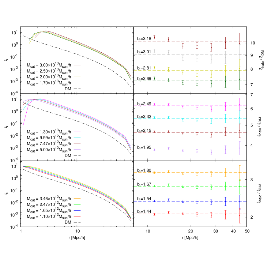
Figure 1: Left: the real-space correlation functions of the halo catalogues, compared to that of the dark-matter particles in the BASICC simulation. Right: the ratio of $\xi_{halo}(r)$ and $\xi_{DM}(r)$ for each catalogue, with the resulting best-fit linear bias $b_{t}^{2}=\xi_{halo}(r)/\xi_{DM}(r)=\text{const}$, fitted over the range $10<r<50\,h^{-1}\,\text{Mpc}$. Error bars correspond to the standard deviation (of the mean) over $27$ sub-cubes.

3.2 Fitting the redshift-space correlation function

We can estimate $\beta$ (and $\sigma_{12}$, for the linear-exponential model) through this modelling, by minimizing the following $\chi^{2}$ function over a spatial grid:

$$\chi^{2}=-2\ln\mathcal{L}=\sum_{i,j}\frac{{(y_{ij}^{(m)}-y_{ij})}^{2}}{\delta_{ij}^{2}}\;,$$ (13)

where $\mathcal{L}$ is the likelihood and we have defined the quantity

$$y_{ij}=\log[1+\xi({r_{p}}_{i},\pi_{j})]\;.$$ (14)

Here the superscript $m$ indicates the model and $\delta^{2}_{ij}$ represents the variance of $y_{ij}$. The use of $\log(1+\xi)$ in Eq. (14) has the advantage of placing more weight on large (linear) scales (Hawkins et al. 2003). However, unlike Hawkins et al. (2003), we simply use the sample variance of $y_{ij}$ to estimate $\delta_{ij}$ (as in Guzzo et al. 2008). We show in Appendix A that this definition provides more stable estimates of $\beta$ also in the low-density regime. The correlation functions are measured using the minimum variance estimator of Landy & Szalay (1993). We tested different estimators, such as Davis & Peebles (1983), Hewett (1982) and Hamilton (1993), finding that our measurements are virtually insensitive to the estimator choice, at least for $r\lesssim 50\ h^{-1}\ \text{Mpc}$. For the linear-exponential model, we perform a two-parameter fit, including the velocity dispersion, $\sigma_{12}$, as a free parameter. However, being our interest here focused on measurements of the growth rate (through $\beta$), $\sigma_{12}$ is treated merely as an extra parameter to (potentially) account for deviations from linear theory.

Finally, in performing the fit we have neglected an important aspect, but for good reasons. In principle, we should consider that the bins of the correlation function are not independent. As such, Eq. (13) should be modified as to include also the contribution of non-diagonal terms in the covariance matrix, i.e. (in matrix form)

$$-2\ln\mathcal{L}={\left({\mathbf{Y}}^{(m)}-{\mathbf{Y}}\right)}^{T}{\mathbf{C}}^{-1}{\left({\mathbf{Y}}^{(m)}-{\mathbf{Y}}\right)}\;,$$ (15)

where ${\mathbf{Y}}$ and ${\mathbf{Y}}^{(m)}$ are two (column) vectors containing all data and model values respectively (with dimension $N_{b}^{2}$, where $N_{b}$ is the number of bins in one dimension used to estimate $\xi(r_{p},\pi)$), whereas ${\mathbf{C}}$ is the covariance matrix, with dimension $N_{b}^{2}\times N_{b}^{2}$.

This is routinely used when fitting 1D correlation functions (e.g. Fisher et al. 1994), but it becomes arduous in the case of the full $\xi(r_{p},\pi)$, for which $N_{b}\approx 100$ and the covariance matrix has $\approx 10^{8}$ elements. What happens in practice, is that the estimated functions are over- sampled, so that the effective number of degrees of freedom in the data is smaller than the number of components in the covariance matrix, which is then singular. Still, a test with as many as 100 blockwise boostrap realizations yields a very unsatisfactory covariance matrix. We tested on a smaller-size $\xi(r_{p},\pi)$ the actual effect of assuming negligible off-diagonal elements in the covariance matrix, obtaining a difference of a few percent in the measured value of $\beta$, as also found in de la Torre & Guzzo (2012). Part of this insensitivity is certainly related to the very large volumes of the mock samples, with respect to the scales involved in the parameter estimations. This corroborates our forced choice of ignoring covariances in the present work, also because of the computational time involved in inverting such large matrices, size multiplied by the huge number of estimates needed for the present work.

3.3 Reference distortion parameters and bias values of the simulated samples

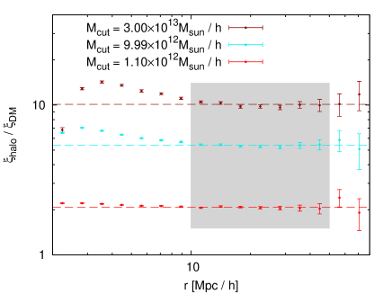
Figure 2: The expected the bias factor, expressed as $b^{2}=\xi_{halo}(r)/\xi_{DM}(r)$, plotted over a wider range of separations than in the previous figure. Dashed lines are obtained by fitting a constant bias model over the range denoted by the grey area, $10<r<50\,h^{-1}\,\text{Mpc}$. Error bars give the standard deviation of the mean over the 27 sub-cubes.

Before measuring the amplitude of redshift distortions in the various samples described above, we need to establish the reference values to which our measurements will be compared, in order to identify systematic effects. Specifically, we need to determine with the highest possible accuracy the intrinsic “true” value of $\beta$ for all mass-selected samples in the simulation. This can be obtained from the relation (Peebles, 1980; Fry, 1985; Lightman & Schechter, 1990; Wang & Steinhardt, 1998)

$$\beta(z)=\frac{\Omega_{M}^{0.55}(z)}{b(z)}\;,$$ (16)

where, $f(z)=\Omega_{M}^{0.55}(z)$ is the growth rate of fluctuations at the given redshift. For the flat cosmology of the simulation $\Omega_{M}(z)$ is

$$\Omega_{M}(z)=\frac{{(1+z)}^{3}\Omega_{M0}}{{(1+z)}^{3}\Omega_{M0}+(1-\Omega_{M0})}\;.$$ (17)

The linear bias can be estimated as

$$b^{2}=\dfrac{\xi_{halo}(r)}{\xi_{DM}(r)}\;.$$ (18)

Here $\xi_{halo}$ and $\xi_{DM}$ have to be evaluated at large separations, $r\gtrsim 10\,h^{-1}\,\text{Mpc}$, where the linear approximation holds. In the following we shall adopt the notation $b_{t}$ and $\beta_{t}$ for the values thus obtained. To recover the bias and its error for each $M_{cut}$ listed in Table 1 we split each cubic catalogue of halos into 27 sub-cubes. Figure 1 shows the measured two-point correlation functions and the corresponding bias values for the various sub-samples. These are computed at different separations $r$, as the average over 27 sub-cubes, with error bars corresponding to the standard deviation of the mean. Dashed lines give the corresponding value of $b_{t}^{2}$, obtained by fitting a constant over the range $10<r<50\,h^{-1}\,\text{Mpc}$. In most cases, the bias functions show a similar scale dependence, but the fluctuations are compatible with scale-independence within the error bars (in particular for halo masses $M_{cut}\leq 1.70\times 10^{13}\ h^{-1}\ M_{\odot}$). For completeness, in Figure 2 we show that this remains valid on larger scales ($r\gtrsim 50\,h^{-1}\,\text{Mpc}$, whereas on small scales ($r\lesssim 10\,h^{-1}\,\text{Mpc}$), a significant scale-dependence is present. The linear bias assumption is therefore acceptable for $r\gtrsim 10\,h^{-1}\,\text{Mpc}$.

In a realistic scenario, $\beta$ is measured from a redshift survey. Then the growth rate is recovered as $f=b\beta$. Unfortunately in a real survey it is not possible to estimate $b$ through Eq. (18) as we described above (and as it is done for dark matter simulations) since the real observable is the two-point correlation function of galaxies, whereas $\xi_{DM}$ cannot be directly observed. A possible solution is to assume a model for the dependence of the bias on the mass. Using groups/clusters in this context may be convenient as their total (DM) mass can be estimated from the X-ray emission temperature or luminosity. We compare our directly measured $b$ with those calculated from two popular models: Sheth, Mo, & Tormen (2001) and Tinker et al. (2010) (hereafter SMT01 and T+10), in Figure 3. Details on how we compute $b_{SMT01}$ and $b_{T+10}$ are reported in the parallel paper by Marulli et al. (2012). We see that for small/intermediate masses our measurements are in good agreement with T+10, whereas for larger masses, $M_{cut}\gtrsim 2\times 10^{13}\ h^{-1}\ M_{\odot}$, SMT01 yields a more reliable prediction of the bias.

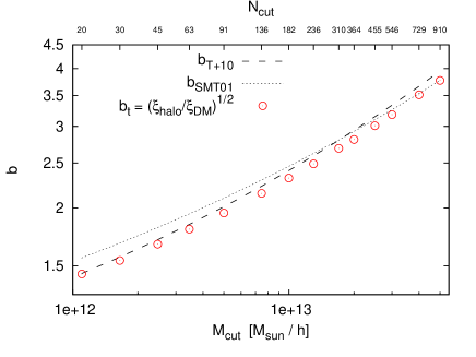
Figure 3: Comparison of the bias values measured from the simulated catalogues as a function of their threshold mass, $M_{cut}$, with the predictions of the SMT01 and T+10 models. The top axis also reports the number of particles per halo, $N_{cut}$, corresponding to the catalogue threshold mass.

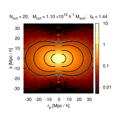
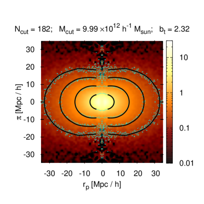
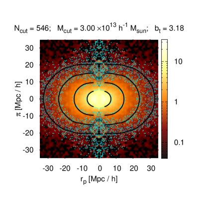
Figure 4: $\xi(r_{p},\pi)$ for the catalogues with $M_{cut}=1.10\times 10^{12}\ h^{-1}\ M_{\odot}$ (upper panel), $M_{cut}=9.99\times 10^{12}\ h^{-1}\ M_{\odot}$ (central panel) and $M_{cut}=3.00\times 10^{13}\ h^{-1}\ M_{\odot}$ (lower panel). Iso-correlation contours of the data are shown in cyan, whereas the best fit model corresponds to the black curves. Note that the color scale and contour levels differ in the three panels. The latter are arbitrarily set to {0.07, 0.13, 0.35, 1}, {0.15, 0.3, 0.7, 2.8} and {0.25, 0.5, 1.3, 5} respectively from top to bottom. When the mass grows, the distortion parameter $\beta$ (i.e. the compression of the pattern along the line of sight) decreases, whereas the correlation and the shot-noise increase.

4 Systematic errors in measurements of the growth rate

4.1 Fitting the linear-exponential model

As in the previous section, we split each of the 12 mass-selected halo catalogues of Table 1 into 27 sub-cubes. Then we compute the redshift-space correlation function $\xi(r_{p},\pi)$ for each of them. Figure 4 gives an example of three cases of different mass. Following the procedure described in Section 3.2, we obtain an estimate of the distortion parameter $\beta$. The 27 values of $\beta$ are then used to estimate the mean value and standard deviation of $\beta$ as a function of the mass threshold (i.e. bias). With the adopted setup (binning and range), the fit becomes unstable for $M_{cut}>3\times 10^{13}\ h^{-1}\ M_{\odot}$, in the sense of yielding highly fluctuating values for $\beta$ and its scatter. Very probably, this is due to the increasing sparseness of the samples and the reduced amplitude of the distortion (since $\beta\propto 1/b$). Figure 4 explicitly shows these two effects: when the mass grows (top to bottom panels) the shot-noise, which depends on the number density, increases, whereas the compression along the line of sight decreases, since it depends on the amplitude of $\beta$. For this reason, in this work we consider only catalogues below this mass threshold, as listed in Table 1.

Figure 5 summarizes our results. The plot shows the mean values of $\beta$ for each mass sample, together with their confidence intervals (obtained from the scatter of the sub-cubes), compared to the expected values of the simulation $\beta_{t}$ (also plotted with their uncertainties, due to the error on the measured bias $b_{t}$, Section 3.3). These have been obtained using the linear-exponential model, Eq. (11), which represents the standard approach in previous works, fitting over the range $3<r_{p}<35\,h^{-1}\text{Mpc}$, $0<\pi<35\,h^{-1}\text{Mpc}$ with linear bins of $0.5\,h^{-1}\text{Mpc}$. We also remark that here the model is built using the “true” $\xi(r)$ measured directly in real-space, which is not directly observable in the case of real data. This is done as to clearly separate the limitations depending on the linear assumption, from those introduced by a limited recontruction of the underlying real-space correlation function. In Appendix B we shall therefore discuss separately the effects of deriving $\xi(r)$ directly from the observations.

Despite the apparently very good fits (Fig. 4), we find a systematic discrepancy between the measured and the true value of $\beta$. The systematic error is maximum ($\approx 10\%$) for low-bias (i.e. low mass) halos and tends to decrease for larger values (note that here with “low bias” we indicate galaxy-sized halos with $M\approx 10^{12}\ h^{-1}\ M_{\odot}$). In particular for $M_{cut}$ between $7\times 10^{12}$ and $\approx 10^{13}\ h^{-1}\ M_{\odot}$ the expectation value of the measurement is very close to the true value $\beta_{t}$.

It is interesting, and somewhat surprising, that, although massive halos are intrinsically sparser (and hence disfavoured from a statistical point of view), the scatter of $\beta$ (i.e. the width of the green error corridor in Figure 5) does not increase in absolute terms, showing little dependence on the halo mass. Since the value of $\beta$ is decreasing, however, the relative error does have a dependence on the bias, as we shall better discuss in § 5.

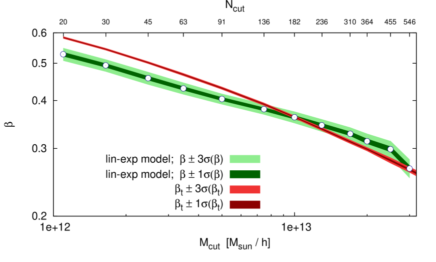
Figure 5: The mean values of $\beta$ averaged over 27 sub-cubes, as measured in each mass sample (open circles) estimated using the “standard” linear-exponential model of Eq. (11). The dark- and light-green bands give respectively the $1\sigma$ and $3\sigma$ confidence intervals around the mean. The measured values are compared to the expected values $\beta_{t}$, computed using Eqs. (16-18). We also give the $1\sigma$ and $3\sigma$ theoretical uncertainty around $\beta_{t}$, due to the uncertainty in the bias estimate ( brown and red bands, respectively).

4.2 Is a pure Kaiser model preferable for cluster-sized halos?

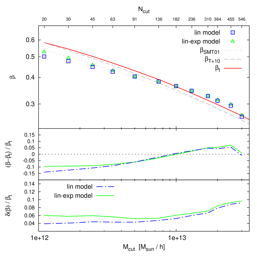
Figure 6: Comparison of the performances of the linear and linear-exponential models. Upper panel: measurements of $\beta$ from the different halo catalogues, obtained wth the linear model of Eq. (5) (squares) and the linear-exponential model of Eq. (11) (trianglesl). Mean values and errors are computed as in Fig. 5 from the 27 sub-cubes of each catalogue. We also plot the expected values of $\beta$ from the simulation, $\beta_{t}=f/b_{t}$ (i.e. $\beta$ “true”) and from the models of Fig. 3, $\beta_{T+10}=f/b_{T+10}$ and $\beta_{SMT01}=f/b_{SMT01}$. Central panel: relative systematic error. Lower panel: relative statistical error.

Groups and clusters would seem to be natural candidates to trace large-scale motions based on a purely linear description, since they essentially trace very large scales and most non-linear velocities are confined within their structure. Using clusters as test particles (i.e. ignoring their internal degrees of freedom) we are probing mostly linear, coherent motions. It makes sense therefore to repeat our measurements using the linear model alone, without exponential damping correction. The results are shown in Figure 6. The relative error (lower panel) obtained in this case is in general smaller than when the exponential damping is included. This is a consequence of the fact that the linear model depends only on one free parameter, $\beta$, whereas the linear-exponential model depends on two free parameters, $\beta$ and $\sigma_{12}$. Both models yield similar systematic error (central panel), except for the lower mass cutoff range where the exponential correction clearly has a beneficial effect. In the following we briefly summarize how relative and systematic errors combine. To do this we consider three different mass ranges arbitrarily choosen.

1. Small masses ($M_{cut}\lesssim 5\times 10^{12}\ h^{-1}M_{\odot}$)
   This range corresponds to halos hosting single $L^{*}$ galaxies. Here the linear exponential model, which gives a smaller systematic error, is still not able to recover the expected value of $\beta$. However, any consideration about these “galactic halos” may not be fully realistic since our halo catalogues are lacking in sub-structure (see Section 4.4).

2. Intermediate masses
                 ($5~{}\times~{}10^{12}\lesssim M_{cut}\lesssim 2~{}\times~{}10^{13}\ h^{-1}~{}M_{\odot}$)
   This range corresponds to halos hosting very massive galaxies and groups. The systematic error is small compared to that of the other mass ranges, for both models. This means that we are free to use the linear model, which always gives a smaller statistical error (lower panel), without having to worry too much about its systematic error, which in any case is not larger than that of the more complex model. In particular, we notice that using the simple linear model in this mass range, the statistical error on $\beta$ is comparable to that obtained with a galaxy-mass sample using the more phenomenological linear-exponential model. This may be a reason for preferring the use of this mass range for measuring $\beta$.

3. Large masses ($M_{cut}\gtrsim 2\times 10^{13}\ h^{-1}M_{\odot}$)
   This range corresponds to halos hosting what we may describe as large groups or small clusters. The random error increases rapidly with mass (Figure 6, lower panel), regardless of the model, due to the reduction of the distortion signal ($\beta\propto 1/b$) and to the decreasing number density.

4.3 Origin of the systematic errors

The results of the previous two sections are not fully unexpected. It has been evidenced in a number of recent papers that the standard linear Kaiser description of RSD, Eq. (4), is not sufficiently accurate on the quasi-linear scales ($\approx 5\div 50\ \text{h}^{-1}\ \text{Mpc}$) where it is normally applied (Scoccimarro 2004; Tinker, Weinberg, & Zheng 2006; Taruya, Nishimichi, & Saito 2010; Jennings, Baugh, & Pascoli 2011; Okumura & Jing 2011; Kwan, Lewis, & Linder 2012). This involves not only the linear model, but also what we called the linear-exponential model. Since the pioneering work of Davis & Peebles (1983) the exponential factor is meant to include the small-scale non-linear motions, but this is in fact empirical and only partially compensates for the inaccurate non-linear description. The systematic error we quantified with our simulations is thus most plausibly interpreted as due to the inadequacy of this model on such scales. Various improved non-linear corrections are proposed in the quoted papers, although their performance in the case of real galaxies still requires further refinement (e.g. de la Torre & Guzzo 2012). On the other hand, considering larger and larger (i.e. more linear) scales, one would expect to converge to the Kaiser limit. In this regime, however, other difficulties emerge, as specifically the low clustering signal, the need to model the BAO peak and the wide-angle effects (Samushia, Percival, & Raccanelli, 2012). We have explored this, although not in a systematic way. We find no indication for a positive trend in the sense of a reduction of the systematic error when increasing the minimum scale $r_{min}$ included in the fit, at least for $r_{min}=20\ h^{-1}\ \text{Mpc}$. Systematic errors remain present, while the statistical error increases dramatically. The situation improves only in a relative sense, because statistical error bars become larger than the systematic error. This is seen in more detail in the parallel work by de la Torre & Guzzo (2012). Finally, it is interesting to remark the indication that systematic errors can be reduced by using the Kaiser model on objects that are intrinsically more suitable for a fully linear description.

4.4 Role of sub-structure: analysis of the Millennium mocks

In the simulated catalogues we use here, sub-structures inside halos, i.e. sub-halos, are not resolved, due to the use of a single linking length when running the Friends-of-Friends algorithm (Section 2.1). As such, the catalogues do not in fact reproduce correctly the small-scale dynamics observed in real surveys. Although we expect that our fit (limited to scales $r_{p}>3\ h^{-1}\ \text{Mpc}$) is not directly sensitive to what happens on the small scales where cluster dynamics dominate, we have decided to perform here a simple direct check of whether these limitations might play a role on the results obtained. Essentially, we want to understand if the absence of sub-structure could be responsible for the enhanced systematic error we found for the low-mass halos.

To this end, we further analysed $100$ Millennium mock surveys. These are obtained by combining the output of the pure dark-matter Millennium run (Springel et al. 2005) with the Munich semi-analytic model of galaxy formation (De Lucia & Blaizot, 2007). The Millennium Run is a large dark matter N-body simulation which traces the hierarchical evolution of $2160^{3}$ particles between $z=127$ and $z=0$ in a cubic volume of $500^{3}~{}h^{-3}~{}\text{Mpc}^{3}$, using the same cosmology of the BASICC simulation $(\Omega_{M},~{}\Omega_{\Lambda},~{}\Omega_{b},~{}h,~{}n,~{}\sigma_{8})=(0.25,~{}0.75,~{}0.045,~{}0.73,~{}1,~{}0.9)$. The mass resolution, $8.6\times 10^{8}~{}h^{-1}M_{\odot}$ allows one to resolve halos containing galaxies with a luminosity of $0.1L^{*}$ with a minimum of 100 particles. Details are given in Springel et al. (2005). The one hundred mocks reproduce the geometry of the VVDS-Wide “F22” survey analysed in Guzzo et al. (2008) (except for the fact that we use complete samples, i.e. with no angular selection function), covering $2\times 2\ \text{deg}^{2}$ and $0.7<z<1.3$. Clearly, these samples are significantly smaller than the halo catalogues built from the BASICC simulations, yet they describe galaxies in a more realistic way and allow us to study what happens on small scales. In addition, while the BASICC halo catalogues are characterized by a well-defined mass threshold, the Millennium mocks are meant to reproduce the selection function of an $I_{AB}<22.5$ magnitude-limited survey like VVDS-Wide. From each of the 100 light cones, we further consider only galaxies lying at $0.7<z<1.3$ to have a median redshift close to unity. The combination of these two sets of simulations should hopefully provide us with enough information to disentangle real effects from artifacts.

Performing the same kind of analysis applied to the BASICC halo catalogues (Figure 7), we find a comparable systematic error, corresponding to an under-estimate of $\beta$ by 10%. We recover $\beta=0.577\pm 0.018$, against an expected value of $\beta_{t}=0.636\pm 0.006$, suggesting that our main conclusions are substantially unaffected by the limited description of sub-halos in the BASICC samples. Another potential source of systematic errors in the larger simulations could be resolution: the dynamics of the smaller halos could be unrealistic simply because they contain too few dark-matter particles. Our results from the Millennium mocks and those of Okumura & Jing (2011), which explicitly tested for such effects, seem however to exclude this possibility.

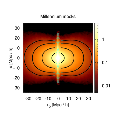
Figure 7: $\xi(r_{p},\pi)$ for the Millennium mocks. The coding is the same as in Fig. 4, with iso-correlation contours arbitrarily set to {0.05, 0.1, 0.25, 1}.

5 Forecasting statistical errors in future surveys

A galaxy redshift survey can be essentially characterized by its volume $V$ and the number density, $n$, and bias factor, $b$, of the galaxy population it includes (besides more specific effects due to sample geometry or selection criteria). The precision in determining $\beta$ depends on these parameters. Using mock samples from the Millennium run similar to those used here, Guzzo et al. (2008) calibrated a simple scaling relation for the relative error on $\beta$, for a sample with $b=1.3$:

$$\dfrac{\delta(\beta)}{\beta}\approx\dfrac{50}{n^{0.44}V^{0.5}}\;,$$ (19)

While a general agreement has been found comparing this relation to Fisher matrix predictions (White, Song, & Percival, 2009), this formula was strictly valid for the limited density and volume ranges originally covered in that work. For example, the power-law dependence on the density cannot realistically be extended to arbitrarily high densities, as also pointed out by Simpson & Peacock (2010). In this section we present the results of a more systematic investigation, exploring in more detail the scaling of errors when varying the survey parameters. This will include also the dependence on the bias factor of the galaxy population. In general, this approach is expected to provide a description of the error budget which is superior to a Fisher matrix analysis, as it does not make any specific assumption on the nature of the errors. All model fits presented in the following sections are performed using the real-space correlation function $\xi(r)$ recovered from the “observed” $\xi(r_{p},\pi)$. This is done through the projection/de-projection procedure described in Appendix B (with $\pi_{max}=25\ h^{-1}\text{Mpc}$), which as we show increases the statistical error by a factor around 2. The goal here is clearly to be as close as possible to the analysis of a real data set.

5.1 An improved scaling formula

$n\times 10^{5}\,[h^{3}\,\text{Mpc}^{-3}]$

311

204

131

90.0

58.7

36.0

24.8

17.6

12.1

9.58

6.87

$1.10\times 10^{12}$

◦

•

•

◦

•

•

◦

•

•

•

•

$1.44$

$1.65\times 10^{12}$

•

•

•

•

•

•

•

•

•

•

$1.54$

$2.47\times 10^{12}$

•

•

•

•

•

•

•

•

•

$1.67$

$3.46\times 10^{12}$

•

•

•

◦

•

•

•

•

$1.80$

$5.00\times 10^{12}$

•

•

•

•

•

•

•

$1.95$

$M_{cut}\ [h^{-1}\ M_{\odot}]$

$7.47\times 10^{12}$

•

•

•

•

•

•

$2.15$

$b$

$9.99\times 10^{12}$

◦

•

•

•

•

$2.32$

$1.30\times 10^{13}$

•

•

•

•

$2.49$

$1.70\times 10^{13}$

•

•

•

$2.69$

$2.00\times 10^{13}$

•

•

$2.81$

$2.50\times 10^{13}$

•

$3.01$

Table 2: Properties of the diluted sub-samples constructed to test the dependence of the error of $\beta$ on bias and mean density. Each entry in the table is uniquely defined by a pair $(M_{cut},n)$; moving along rows or columns the samples keep a fixed bias (mass threshold) or density, respectively. Bias values are explicitly reported at the right-hand side of the table. The diagonal coincides with the full (i.e. non-diluted) samples. Empty circles indicate catalogues which have been used also to test the dependence on the volume: they have been split into $N_{split}^{3}$ sub-samples for $N_{split}=3,4,5,6$, whereas all other catalogues (filled circles) use $N_{split}=3$ only for the sake of building statistical quantities.

In doing this exercise, a specific problem is that, as shown in Table 1, catalogues with larger mass (i.e. higher bias) are also less dense. Our aim is to separate the dependence of the errors on these two variables. To do so, once a population of a given bias is defined by choosing a given mass threshold, we construct a series of diluted samples obtained by randomly removing objects. The process is repeated down to a minimum density of $6.87\times 10^{-5}\ h^{3}\ \text{Mpc}^{-3}$, at which shot noise dominates and for the least massive halos the recovered $\beta$ is consistent with zero. In this way, we obtain a series of sub-samples of varying density for fixed bias, as reported in Table 2. The full samples are the same used to build, e.g., Figure 5.

In Figure 8 we plot the relative errors on $\beta$ measured from each catalogue of Table 2, as a function of the bias factor and the number density. These 3D plots are meant to provide an overview of the global behavior of the errors; a more detailed description is provided in Figures 10-11, where 2D sections along $n$ and $b$ are reported. For all the samples considered, the volume is held fixed.

As shown by the figure, the bias dependence is weak and approximately described by $\delta(\beta)/\beta\propto b^{0.7}$, i.e. the error is slightly larger for higher-bias objects. This indicates that the gain of a stronger clustering signal is more than cancelled by the reduction of the distortion signal, when higher bias objects are considered. This is however fully true only for samples which are not too sparse intrinsically. We see in fact that at extremely low densities, the relationship is inverted, with high-bias objects becoming favoured. At the same time, there is a clear general flattening of the dependence of the error on the mean density $n$. The relation is not a simple power-law, but becomes constant at high values of $n$. In comparison, over the density range considered here, the old scaling formula of Guzzo et al. would overestimate the error significantly. This behaviour is easily interpreted as showing the transition from a shot-noise dominated regime at low densities to a cosmic-variance dominated one, in which there is no gain in further increasing the sampling. Such behaviour is clear for low-mass halos (i.e. low bias) but is much weaker for more massive, intrinsically rare objects.

Figure 8: Dependence of the relative error of $\beta$ on the bias and number density of the catalogues in Table 2, overplotted on the surface described by the scaling formula of Eq. (20). While the left panel is intended to give an overall view, the right panel is expressly oriented to show that the formula is an excellent description of the data.

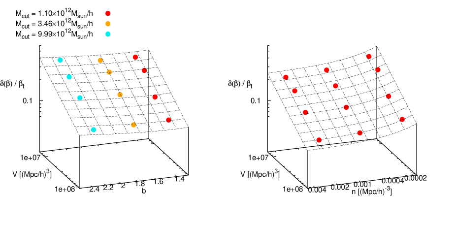
Figure 9: Relative error on $\beta$ as a function of volume, bias and number density. The dependence on volume is explored by dividing the sample into $N_{split}^{3}$ sub-samples, with $N_{split}=3,4,5,6$. As in all of this section, in modelling the measured $\xi(r_{p},\pi)$ through Eq. (11) we use the deprojected $\xi(r)$ (with $\pi_{max}=25\ h^{-1}\text{Mpc}$), as to represent a condition as close as possible to real observations. The superimposed grid is described by the scaling formula of Eq. (20). Left panel: $\delta(\beta)/\beta_{t}$ as a function of volume and bias, considering three different threshold masses (i.e. biases), but randomly diluting the catalogues as to keep a constant number density, $n=2.48\times 10^{-4}\,h^{3}\,\text{Mpc}^{-3}$ in all cases (see Table 2, empty circles). Right panel: $\delta(\beta)/\beta_{t}$ as a function of the volume, $V$, and the number density, $n$. Here we consider a single threshold mass, $M_{cut}=1.10\times 10^{12}\ h^{-1}\ M_{\odot}$, corresponding to a constant bias, $b=1.44$.

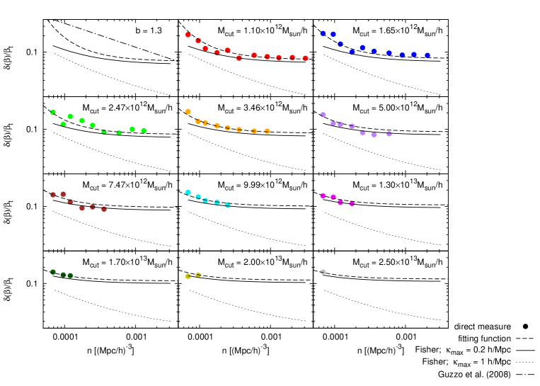
Figure 10: The relative error on $\beta$ as a function of the mean number density of the sample, predicted with the Fisher matrix approach (solid and dotted lines) and measured from the simulated samples (filled circles; colours coded as in previous figures). The solid and dotted lines correspond to using respectively $k_{max}=0.2\ h\ \text{Mpc}^{-1}$ or $k_{max}=1\ h\ \text{Mpc}^{-1}$ (with Lorentzian damping) in the Fisher forecasts. The dashed lines show in addition the behaviour of the scaling formula obtained from the simulation results (Eq. (20)). This is also compared, in the top-left panel, to the old simplified fitting formula for $b=1.3$ galaxies of Eq. (19).

We can now try to model an improved empirical relation to reproduce quantitatively these observed dependences. Let us first consider the general trend, $\delta(\beta)/\beta\propto b^{0.7}$, which describes well the trend of $\delta(\beta)/\beta$ in the cosmic variance dominated region (i.e. at high density). In Figure 8 such a power-law is represented by a plane. We then need a function capable to warp the plane in the low density region, where the relative error becomes shot-noise dominated. The best choice seems to be an exponential: $\delta(\beta)/\beta\propto b^{0.7}\exp(n_{0}/n)$, where, by construction, $n_{0}$ roughly corresponds to the threshold density above which cosmic variance dominates. Finally, we need to add an exponential dependence on the bias so that at low density the relative error decreases with $b$, such that the full expression becomes $\delta(\beta)/\beta\propto b^{0.7}\exp[n_{0}/(b^{2}n)]$. The grid shown in Figure 8 represents the result of a direct fit of this functional form to the data, showing that it is indeed well suited to describe the overall behaviour. In the right panel we have oriented the axes as to highlight the goodness of the fit: the rms of the residual between model and data is $\approx 0.015$, which is an order of magnitude smaller than the smallest measured values of $\delta(\beta)/\beta$. This gives our equation the predictive power we were looking for: if we use it to produce forecasts of the precision of $\beta$ for a given survey, we shall commit a negligible error ($\lesssim 20\%$) on $\delta(\beta)/\beta$ (at least for values of bias and volume within the ranges tested here). To fully complete the relation, we only need to add the dependence on the volume, which is in principle the easiest. To this end, we split the whole simulation cube into $N_{split}^{3}$ sub-cubes, with $N_{split}=3,4,5,6$. By applying this procedure to 5 samples with different bias and number density (see Table 2) we make sure that our results do not depend on the particular choice of bias and density. Figure 9 shows that $\delta(\beta)/\beta\propto V^{-0.5}$ independently of $n$ and $b$, confirming the dependence found by Guzzo et al. (2008). We can thus finally write the full scaling formula for the relative error of $\beta$ we were seeking for

$$\delta(\beta)/\beta\approx Cb^{0.7}V^{-0.5}\exp\bigg{(}\dfrac{n_{0}}{b^{2}n}\bigg{)}\;,$$ (20)

where $n_{0}=1.7\times 10^{-4}\ h^{3}\ \text{Mpc}^{-3}$ and $C=4.9\times 10^{2}\ h^{-1.5}\ \text{Mpc}^{1.5}$. Clearly, by construction, this scaling formula quantifies random errors, not the systematic ones.

Figure 11: The relative error on $\beta$ as a function of the effective bias factor, predicted by the Fisher matrix (solid and dotted lines) and measured from the simulated samples (filled circles; colours coded as in previous figures). The solid and dotted lines correspond to using respectively $k_{max}=0.2\ h\ \text{Mpc}^{-1}$ or $k_{max}=1\ h\ \text{Mpc}^{-1}$ (with Lorentzian damping) in the Fisher forecasts. The dashed lines show in addition the behaviour of the scaling formula obtained from the simulation results (Eq. (20)).

5.2 Comparison to Fisher matrix predictions

The Fisher information matrix provides a method for determining the sensitivity of a particular experiment to a set of parameters and has been widely used in cosmology. In particular, Tegmark (1997) introduced an implementation of the Fisher matrix aimed at forecasting errors on cosmological parameters derived from the galaxy power spectrum $P(k)$, based on its expected observational uncertainty, as described by Feldman, Kaiser, & Peacock (1994, FKP). This was adapted by Seo & Eisenstein (2003) to the measurements of distances using the baryonic acoustic oscillations in $P(k)$. Following the renewed interest in RSD, over the past few years the Fisher matrix technique has also been applied to predict the errors expected on $\beta$, $f$ and related parameters (e.g Linder, 2008; Wang, 2008; Percival & White, 2009; White, Song, & Percival, 2009; Simpson & Peacock, 2010; Wang et al., 2010; Samushia et al., 2011; Bueno Belloso, García-Bellido, & Sapone, 2011; di Porto, Amendola, & Branchini, 2012). The extensive simulations performed here provides us with a natural opportunity to perform a first simple and direct test of these predictions. Given the number of details that enter in the Fisher matrix implementation, this cannot be considered as exhaustive. Yet, a number of interesting indications emerge, as we shall see.

We have computed Fisher matrices for all catalogues in Table 2, using a code following White, Song, & Percival (2009). In particular, our Fisher matrix predicts errors on $\beta$ and $b$ , given the errors on the linear redshift space power spectrum modeled as in Eq. (4) (Kaiser, 1987). We first limit the computations to linear scales, applying the standard cut-off $k<k_{max}=0.2\ h\ {\rm Mpc}^{-1}$. We also explore the possibility of including wavenumbers as large as $k=\pi/3\sim 1\ h\ {\rm Mpc}^{-1}$ (that should better match the typical scales we fit in the correlation functions from the simulations), accounting for non-linearity through a conventional small-scale Lorentzian damping term. Our fiducial cosmology corresponds to that used in the simulation, i.e. $\Omega_{M}=0.25$, $\Omega_{\Lambda}=0.75$, $H_{0}=0.73$ and $\sigma_{8}=0.9$ today. We also choose $\sigma_{12}=200$ km s^-1 as reference value for the pairwise dispersion. We do not consider geometric distortions (Alcock & Paczynski, 1979), whose impact on RSD is addressed in the parallel paper by Marulli et al. (2012). To obtain the Fisher predictions on $\beta$, we marginalize over the bias, to account for the uncertainty on its precise value, and on the pairwise velocity in the damping term (when present).

Figure 10 shows the measured relative errors on $\beta$ as a function of the number density, compared to the Fisher forecasts for the two choices of $k_{max}$. We also plot the scaling relation from Eq. (20), which best represents the simulation results. We see that the simulation results are in in fairly good agreement with the Fisher predictions, when we limit the computation to very linear scales in the power spectrum (solid line). The inclusion of higher wavenumbers produces unrealistically small errors and with a wrong dependence on the number density. Both the solid lines and points reproduce the observed flattening at high number densities, which corresponds to the transition between a shot-noise and a cosmic-variance dominated regime, respectively.

Similarly, Figure 11 looks at the dependence of the error on the linear bias parameter, comparing the simulation results (points and scaling formula best-fit) to the Fisher forecasts. The behaviour is similar to that observed for the number density: there is a a fairly good agreement when the Fisher predictions are computed using $k_{max}=0.2\ h\ {\rm Mpc}^{-1}$, except for very low values of the number density and the bias. Again, when non-linear scales are included, the Fisher predictions become too optimistic by a large factor.

6 Summary and Discussion

We have performed an extensive investigation of statistical and systematic errors in measurements of the redshift-distortion parameter $\beta$ from future surveys. We have considered tracers of the large-scale distribution of mass with varying levels of bias, corresponding to objects like galaxies, groups and clusters. To this purpose, we have analyzed large catalogues of dark-matter halos extracted from a snapshot of the BASICC simulation at $z=1$. Our results clearly evidence the limitations of the linear description of redshift-space distortions, showing how errors depend on the typical survey properties (volume and number density) and the properties of the tracers (bias, i.e. typical mass). Let us recap them and discuss their main implications.

• Estimating $\beta$ using the Hamilton/Kaiser harmonic expansion of the redshift-space correlation function $\xi(r_{p},\pi)$ extended to typical scales, leads to a systematic error of up to $10\%$. This is much larger than the statistical error of a few percent reachable by next-generation surveys. The larger systematic error is found for small bias objects, and decreases reaching a minimum for halos of $10^{13}\ h^{-1}\ M_{\odot}$. This reinforces the trend observed by Okumura & Jing (2011).

• Additional analysis of mock surveys from the Millennium run confirm that the observed systematic errors are not the result of potentially missing sub-structure in the BASICC halo catalogues.

• The use of the deprojected correlation function increases the statistical error, inducing also some additional systematic effects (details are given in Appendix B and also in the companion paper by Marulli et al. (2012)).

• For highly biased objects, which are sparser and whose surveys typically cover larger, more linear scales, the simple Kaiser model describes fairly well the simulated data, without the need of the empirical damping term with one extra parameter accounting for non-linear motions. This results in smaller statistical errors.

• We have derived a comprehensive scaling formula, Eq. (20), to predict the precision (i.e. relative statistical error) reachable on $\beta$ as a function of survey parameters. This expression improves on a previous attempt (Guzzo et al., 2008), generalizing the prediction to a population of arbitrary bias and properly describing the dependence on the number density.

  This formula can be useful to produce quite general and reliable forecasts for future surveys. One should in any case consider that there are a few implementation-specific factors that can modify the absolute values of the recovered rms errors. For example, these would depend on the range of scales over which $\xi(r_{p},\pi)$ is fitted. The values obtained here refer to fits performed between $r_{min}=3$ and $r_{max}=35\ h^{-1}\ \text{Mpc}$. This has been identified through several experiments as an optimal range to minimize statistical and systematic errors for surveys this size (Bianchi, 2010). Theoretically, one may find natural to push $r_{max}$, or both $r_{min}$ and $r_{max}$ to larger scales, as to (supposedly) reduce the weight of nonlinear scales. In practice, however, in both cases we see that random errors increase in amplitude (while the systematic error is not appreciably reduced).

  Similarly, one should also keep in mind that the formula is strictly valid for $z=1$, i.e. the redshift where it has been calibrated. There is no obvious reason to expect the scaling laws among the different quantities (density, volume, bias) to depend significantly on the redshift. This is confirmed by a few preliminary measurements we performed on halo catalogues from the $z=0.25$ snapshot of the BASICC. Conversely, the magnitude of the errors may change, as shown, e.g., in de la Torre & Guzzo (2012). We expect these effects to be described by a simple renormalization of the constant $C$.

  Finally, one may also consider that the standard deviations measured using the 27 sub-cubes could be underestimated, if these are not fully independent. We minimize this by maximizing the size of each sub-cube, while having enough of them as to build a meaningful statistics. The side of each of the 27 sub-cubes used is in fact close to $500\ h^{-1}\ \text{Mpc}$, benefiting of the large size of the BASICC simulation.

• We have compared the error estimations from our simulations with idealized predictions based on the Fisher matrix approach, customarily implemented in Fourier space. We find a good agreement, but only when the Fisher computation is limited to significantly large scales, i.e. $k<k_{max}=0.2\ h\ {\rm Mpc}^{-1}$. When more non-linear scales are included (as an attempt to roughly match those actually involved in the fitting of $\xi(r_{p},\pi)$ in configuration space), then the predicted errors become unrealistically small. This indicates that the usual convention of adopting $k_{max}\sim 0.2\ h\ {\rm Mpc}^{-1}$ for these kind of studies is well posed. On the other hand, it seems paradoxical that in this way with the two methods we are looking at different ranges of scales. The critical point clearly lies in the idealized nature of the Fisher matrix technique. When moving up with $k_{max}$ and thus adding more and more nonlinear scales, the Fisher technique simply accumulates signal and dramatically improves the predicted error, clearly unaware of the additional “noise” introduced by the breakdown of linearity. On the other hand, if in the direct fit of $\xi(r_{p},\pi)$ (or $P(k,\mu)$) one conversely considers a corresponding very linear range $r>2\pi/k_{max}\sim 30\ h^{-1}\ \text{Mpc}$, a poor fit is obtained, with much larger statistical errors than shown, e.g., in Fig. 5. There is no doubt that smaller, mildly nonlinear scales at intermediate separations have necessarily to be included in the modelling if one aims at reaching percent statistical errors on measurements of $\beta$ (or $f$). If one does this in the Fisher matrix, then the predicted errors are too small. The need to push our estimates to scales which are not fully linear will remain true even with surveys of the next generation, including tens of millions of galaxies over Gpc volumes, because that is where the clustering and distortion signals are (and will still be) the strongest. Of course, our parallel results on the amount of systematic errors that plague estimates based on the standard dispersion model also reinforce the evidence that better modelling of nonlinear effects is needed on these scales. The strong effort being spent in this direction gives some confidence that significant technical progress will happen in the coming years (see e.g. Kwan, Lewis, & Linder, 2012; de la Torre & Guzzo, 2012, and references therein).

  In any case, this limited exploration suggests once more that forecasts based on the Fisher matrix approach, while giving useful guidelines evidence the error dependences, have to be treated with significant caution and possibly verified with more direct methods. Similar tension between Fisher and Monte Carlo forecasts has been recently noticed by Hawken et al. (2012).

• Finally, in Appendix A we have also clarified which is the most unbiased form to be adopted for the likelihood when fitting models to the observed redshift-space correlation function, proposing a slightly different form with respect to previous works.

With redshift-space distortions having emerged as probe of primary interest in current and future dark-energy-oriented galaxy surveys, the results presented here further stress the need for improved descriptions of non-linear effects in clustering and dynamical analyses. On the other hand, they also indicate the importance of building surveys for which multiple tracers of RSD (with different bias values) can be identified and used in combination to help understanding and minimizing systematic errors.

Appendix A Definition of the likelihood function to estimate $\beta$

To estimate $\beta$, in Section 3.2 we defined a likelihood function comparing the measured correlation function $\xi(r_{p},\pi)$ and the corresponding parameterized models. Our likelihood is simply given by the standard $\chi^{2}$ expression

$$-2\ln\mathcal{L}=\sum_{i,j}\frac{{(y_{ij}^{(m)}-y_{ij})}^{2}}{\delta_{ij}^{2}}\;,$$ (21)

where however the stochastic variable considered is not just the value of $\xi(r_{p},\pi)$ at each separation $(r_{p},\pi)=(r_{i},r_{j})$, but the expression

$$y_{ij}=\log[1+\xi(r_{i},r_{j})]\;,$$ (22)

which has the desirable property of placing more weight on large, more linear scales. This was first proposed by Hawkins et al. (2003), who correspondingly adopt the following expression for the expectation value of the variance

$$\delta_{ij}^{2}={\{\log[1+\xi_{ij}+\delta(\xi_{ij})]-\log[1+\xi_{ij}-\delta(\xi_{ij})]\}}^{2}\;.$$ (23)

This simply maps onto the new variables $y_{ij}$, the interval including 68% of the distribution in the original variables $\xi_{ij}$, i.e. twice the standard deviation if this were Gaussian distributed. Strictly speaking, here an extra factor 1/2 would be formally required if one aims at defining the equivalent of a standard deviation, but this is in the end uneffective in the minimization and thus in finding the best-fitting parameters.

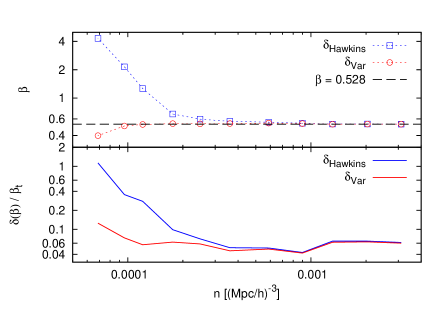
Figure 12: Mean value (top) and relative scatter (bottom) of $\beta$, as recovered from catalogues with varying density (but same volume and bias), using the two different definitions of the variance of each data point of Eqs. 23 (open blue squares) and  24 (open red circles). The dashed line shows as reference the asymptotic common value of $\beta$ that both methods identically recover at high densities. Note how using eq.  24 yields an unbiased estimate down to significantly smaller densities, whereas the estimator based on Eq. (23) becomes rapidly more and more biased below $n\approx 5\times 10^{-4}\ h^{3}\ \text{Mpc}^{-3}$. The intrinsic scatter of the measurements, as usual obtained from the 27 sub-cubes of this specific catalogue, also follows a similar trend.

However, the weighting factors $1/\delta_{ij}$ in the likelihood definition depend explicitly on $\xi_{ij}$, which may result in an improper weighting of the data when the correlation signal fluctuates near zero. We have directly verified that when the estimate is noisy, it is preferable to use a smooth weighting scheme rather than one that is sensitive to local random oscillations of $\xi$, which is more likely to yield biased estimates. This supported our choice of adopting the usual sample-variance expression

$$\delta_{ij}^{2}=\frac{1}{N}\sum_{k}\left(y_{ij}^{(k)}-\left<y_{ij}\right>\right)^{2}\;,$$ (24)

estimated over $N$ realizations of the survey. This can be done using mock realizations (Guzzo et al., 2008), or, alternatively, through appropriate jack-knife or booststrap resamplings of the data. Specifically, we find a significant advantage of the weighting scheme based on sample variance when dealing with low-density samples. This is shown in Figure 12, where $\beta$ is estimated on the catalogue with $M_{cut}=1.10\times 10^{12}\ h^{-1}\ M_{\odot}$ using the two likelihoods and gradually diluting the sample (note that all computations in this section use the linear-exponential model, with $\xi(r)$ directly measured in real-space).

In order to understand the reasons behind this behaviour, we have studied independently the various terms composing the likelihood. We use one single sub-cube (i.e. 1/27 of the total volume), from the catalogue with $M_{cut}=1.10\times 10^{12}\ h^{-1}\ M_{\odot}$, and consider two extreme values of the mean density. First, we consider the case of the highest density achievable by this halo catalogue, $n=3.11\times 10^{-3}\,h^{3}\,\text{Mpc}^{-3}$. In the upper panel of Figure 13 we plot a section of $\xi(r_{p},\pi)$ at constant $\pi=9.75\,h^{-1}\,\text{Mpc}$, together with the model $\xi_{m}(r_{p},\pi)$ corresponding to the best-fit $\beta$ and $\sigma_{12}$ parameters. In this density regime the values of the recovered best-fit parameters are essentially independent of the form chosen for $\delta_{ij}^{2}$ (as shown by the coincident values of $\beta$ on the right side of Figure 12). The match of the model to the data is very good. In the central panel, we plot instead, for each bin $i$ along $r_{p}$, the absolute value of the difference between model and observation, $\left(|y-y_{m}|\right)_{i}$, together with the corresponding standard deviations in the two cases, which are virtually indistinguishable from each other. Finally, the lower panel shows the full values of the terms contributing to the $\chi^{2}$ sum, again showing the equivalence of the two choices in this density regime.

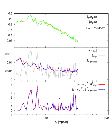
Figure 13: Comparison of the performances of the two likelihood forms discussed in the text in the high-density regime, using the fully sampled population of halos from a single sub-cube (1/27 of the volume) with $M_{cut}=1.10\times 10^{12}\ h^{-1}\ M_{\odot}$. Top panel: cut-through $\xi(r_{p},\pi)$ at fixed $\pi=9.75\,h^{-1}\,\text{Mpc}$ (broken line), and corresponding best fit model $\xi_{m}(r_{p},\pi)$ using the Hawkins et al. form for the scatter of each data point (continuous line). Central panel: residual values $|y_{ij}-y^{(m)}_{ij}|$ between the data and model values (light grey line) and values for the scatter of each point, according to the two definitions of Eqs.  24 (solid red line) and  23 (dashed blue line). Bottom panel: corresponding terms in the $\chi^{2}$ sum (see Eq. (21)). The two definitions for the scatter, as expected, produce virtually identical values for the likelihood.

However, when we sparsely sample the catalogue, as to reach a mean density of $n=9.58\times 10^{-5}$ $h^{3}\,\text{Mpc}^{-3}$ (leaving all other parameters unchanged), a very different behaviour emerges (Figure 14).

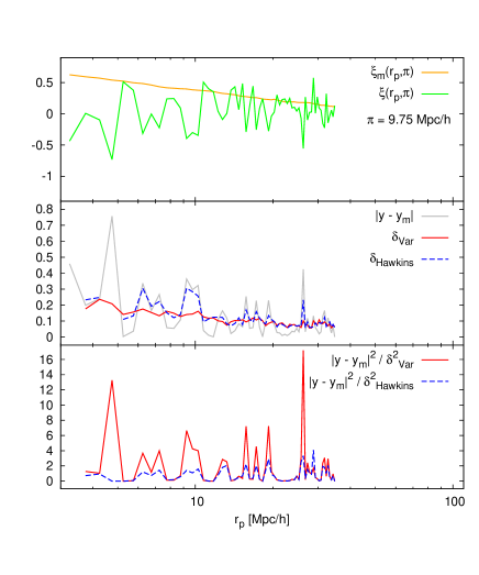
Figure 14: Same as Figure 13, but now in the low-density regime ($n=9.58\times 10^{-5}\,h^{3}\,\text{Mpc}^{-3}$). Again, the model curve in the top panel corresponds to the best-fit parameters obtained using the Hawkins et al. form of the scatter of each measurements. The fit is very unsatisfactory. The bottom panel shows how the likelihood expression based instead on the standard deviation of $y$ as from Eq. (24) rejects these parameter values, giving high $\chi^{2}$ values (red solid curve). Note the different scale on the ordinate, with respect to previous figure.

Using the Hawkins et al. definition for the variance yields a best-fit model that overestimates the data on almost all scales (top panel), corresponding to unphysical values of $\beta=2.33$ and $\sigma_{12}=2112\,\text{km}\,s^{-1}$. The central panel now shows how in this regime the two definitions of the scatter, (which weigh the data-model difference), behave in a significantly different way, with the Hawkins et al. definition being much less stable than the one used here, and in general anti-correlated with the values of $\xi(r_{p},\pi)$ in the upper panel. In the lower panel, the dashed line shows how this anti-correlation smooths down the $(|y-y_{m}|)_{i}$ peaks resulting in erroneously low values for the $\chi^{2}$ that drive the fit to a wrong region of the parameter space. In the same panel, the solid line shows how the likelihood computed with our definition for these same parameters gives high $\chi^{2}$ values, thus correctly rejecting the model.

Appendix B Additional systematic effect when using the deprojected correlation function

In a real survey, the direct measurement of $\xi(r)$ is not possible. A way around this obstacle is to project $\xi(r_{p},\pi)$ along the line of sight, i.e. along the direction affected by redshift distortions. We hence define the projected correlation function as

$$w_{p}(r_{p})=2\int_{0}^{\infty}\xi(r_{p},\pi)d\pi=2\int_{r_{p}}^{\infty}\frac{r^{\prime}\xi(r^{\prime})dr^{\prime}}{\sqrt{r^{\prime 2}-r_{p}^{2}}}\;.$$ (25)

Inverting the integral we recover $\xi(r)$. More precisely, following Saunders, Rowan-Robinson, & Lawrence (1992), we have

$$\xi(r)=\dfrac{1}{\pi}\int_{r}^{\infty}\dfrac{dw_{p}(r_{p})/dr_{p}}{\sqrt{r_{p}^{2}-r^{2}}}dr_{p}\;,$$ (26)

where $\pi$ is the usual mathematical constant, not to be confused with the line-of-sight separation $\pi$ in Eq. (25).

A more extended investigation of the effects arising when using the deprojected $\xi(r)$ instead of that directly measured (hereafter $\xi_{dep}$ and $\xi_{dir}$ respectively) is carried out in Marulli et al. (2012). Here we limit the discussion to the impact of the deprojection technique on the estimate of $\beta$, as a function of the mass (i.e. the bias) of the adopted tracers, focussing on the systematic effects (Figure 15).

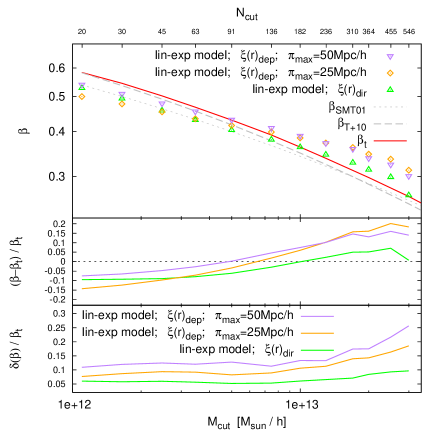
Figure 15: The effect of using the de-projected real-space correlation function in the RSD model. Upper panel: values of $\beta$ obtained when the real-space correlation function $\xi(r)$ is directly measured from the simulation (triangles) or deprojected as in real surveys (rhombs and inverted triangles). The latter correspond to two different integration limits $\pi_{max}$ in the projection. The two lower panels give ths systematic and statistical error as in Figure 6.

One possible source of systematic error in performing the de-projection is the necessity of defining a finite integration limit $\pi_{max}$ in Eq. (26). In Figure 15 two different choices of $\pi_{max}$ are considered. We notice that these choices (purple inverted triangles and yellow rhombs) result in different slopes of $\beta$ as a function of bias, which differ from the slope obtained using $\xi_{dir}$ (green triangles). This is plausibly due to the fact that using a limiting $\pi_{max}$ we are underestimating the integral (consider that $\xi>0$ for $\pi\lesssim 100\ h^{-1}\text{Mpc}$). This effect grows when the bias increases, because of the corresponding growth of $\xi$ which leads to a larger “loss of power” in $w_{p}$. However, we cannot use arbitrarily large values of $\pi_{max}$ because the statistical error increases for larger $\pi_{max}$ (see lowest panel of Figure 15). This may be due to the increase of the shot noise at large separations. Similarly, the drop of correlation signal at small separations due to the finite size of the dark matter halos produces an impact on $\beta$ which grows with bias. Finally, as suggested previously (Guzzo et al., 2008) and discussed extensively in Marulli et al. (2012), Figure 15 shows how using $\xi_{dep}$ in modelling RSD, produces a statistical error about twice as large as that obtained using $\xi_{dir}$ (lower panel).

References

- Acquaviva et al. (2008) Acquaviva V., Hajian A., Spergel D. N., Das S., 2008, PhRvD, 78, 043514
- Alcock & Paczynski (1979) Alcock C., Paczynski B., 1979, Nature, 281, 358
- Angulo et al. (2008) Angulo R. E., Baugh C. M., Frenk C. S., Lacey C. G., 2008, MNRAS, 383, 755
- Angulo & White (2010) Angulo, R.E., White, S.D.M., 2010, MNRAS, 405, 143
- Bianchi (2010) Bianchi D., 2010, Master Laurea Thesis, Unversity of Milan
- Blake et al. (2011) Blake C., et al., 2011, MNRAS, 415, 2876
- Bueno Belloso, García-Bellido, & Sapone (2011) Bueno Belloso A., García-Bellido J., Sapone D., 2011, JCAP, 10, 10
- Cabré & Gaztañaga (2009) Cabré A., Gaztañaga E., 2009, MNRAS, 393, 1183
- Cappelluti et al. (2011) Cappelluti N., et al., 2011, MSAIS, 17, 159
- Davis & Peebles (1983) Davis M., Peebles P. J. E., 1983, ApJ, 267, 465
- Davis et al. (1985) Davis M., Efstathiou G., Frenk C. S., White S. D. M., 1985, ApJ, 292, 371
- de la Torre & Guzzo (2012) de la Torre S., Guzzo L., 2012, arXiv, arXiv:1202.5559
- De Lucia & Blaizot (2007) De Lucia G., Blaizot J., 2007, MNRAS, 375, 2
- di Porto, Amendola, & Branchini (2012) di Porto C., Amendola L., Branchini E., 2012, MNRAS, 419, 985
- Eisenstein et al. (2011) Eisenstein D. J., et al., 2011, AJ, 142, 72
- Feldman, Kaiser, & Peacock (1994) Feldman H. A., Kaiser N., Peacock J. A., 1994, ApJ, 426, 23
- Fisher et al. (1994) Fisher K. B., Davis M., Strauss M. A., Yahil A., Huchra J., 1994, MNRAS, 266, 50
- Fisher et al. (1994) Fisher K. B., Davis M., Strauss M. A., Yahil A., Huchra J. P., 1994, MNRAS, 267, 927
- Fry (1985) Fry J. N., 1985, PhLB, 158, 211
- Guzzo et al. (2008) Guzzo L., et al., 2008, Nature, 451, 541
- Hamilton (1992) Hamilton A. J. S., 1992, ApJ, 385, L5
- Hamilton (1993) Hamilton A. J. S., 1993, ApJ, 417, 19
- Hamilton (1998) Hamilton, A. J. S. 1998, in D. Hamilton, ed, The Evolving Universe. Kluwer, Dordrecht, p. 185
- Hawken et al. (2012) Hawken A. J., Abdalla F. B., Hütsi G., Lahav O., 2012, MNRAS, 424, 2
- Hawkins et al. (2003) Hawkins E., et al., 2003, MNRAS, 346, 78
- Hewett (1982) Hewett P. C., 1982, MNRAS, 201, 867
- Jenkins et al. (2001) Jenkins A., Frenk C. S., White S. D. M., Colberg J. M., Cole S., Evrard A. E., Couchman H. M. P., Yoshida N., 2001, MNRAS, 321, 372
- Jennings, Baugh, & Pascoli (2011) Jennings E., Baugh C. M., Pascoli S., 2011, MNRAS, 410, 2081
- Kaiser (1987) Kaiser N., 1987, MNRAS, 227, 1
- Kwan, Lewis, & Linder (2012) Kwan J., Lewis G. F., Linder E. V., 2012, ApJ, 748, 78
- Landy & Szalay (1993) Landy S. D., Szalay A. S., 1993, ApJ, 412, 64
- Larson et al. (2011) Larson D., et al., 2011, ApJS, 192, 16
- Laureijs et al. (2011) Laureijs R., et al., 2011, arXiv, arXiv:1110.3193
- Lightman & Schechter (1990) Lightman A. P., Schechter P. L., 1990, ApJS, 74, 831
- Linder (2008) Linder E. V., 2008, APh, 29, 336
- Marulli et al. (2012) Marulli F., Bianchi D., Branchini E., Guzzo L., Moscardini L., Angulo R. E., 2012, MNRAS, 426, 2566
- McDonald & Seljak (2009) McDonald P., Seljak U., 2009, JCAP, 10, 7
- Nesseris & Perivolaropoulos (2008) Nesseris S., Perivolaropoulos L., 2008, PhRvD, 77, 023504
- Okumura & Jing (2011) Okumura T., Jing Y. P., 2011, ApJ, 726, 5
- Peacock (1999) Peacock J. A., 1999, Cosmological Physics, Cambridge Univ. Press, Cambridge
- Peebles (1980) Peebles P. J. E., 1980, lssu.book,
- Percival & White (2009) Percival W. J., White M., 2009, MNRAS, 393, 297
- Percival et al. (2010) Percival W. J., et al., 2010, MNRAS, 401, 2148
- Perlmutter et al. (1999) Perlmutter S., et al., 1999, ApJ, 517, 565
- Riess et al. (1998) Riess A. G., et al., 1998, AJ, 116, 1009
- Samushia et al. (2011) Samushia L., et al., 2011, MNRAS, 410, 1993
- Samushia, Percival, & Raccanelli (2012) Samushia L., Percival W. J., Raccanelli A., 2012, MNRAS, 420, 2102
- Sánchez et al. (2006) Sánchez A. G., Baugh C. M., Percival W. J., Peacock J. A., Padilla N. D., Cole S., Frenk C. S., Norberg P., 2006, MNRAS, 366, 189
- Saunders, Rowan-Robinson, & Lawrence (1992) Saunders W., Rowan-Robinson M., Lawrence A., 1992, MNRAS, 258, 134
- Scoccimarro (2004) Scoccimarro R., 2004, PhRvD, 70, 083007
- Seo & Eisenstein (2003) Seo H.-J., Eisenstein D. J., 2003, ApJ, 598, 720
- Sheth, Mo, & Tormen (2001) Sheth R. K., Mo H. J., Tormen G., 2001, MNRAS, 323, 1
- Simpson & Peacock (2010) Simpson F., Peacock J. A., 2010, PhRvD, 81, 043512
- Song & Percival (2009) Song Y.-S., Percival W. J., 2009, JCAP, 10, 4
- Springel et al. (2005) Springel V., et al., 2005, Natur, 435, 629
- Taruya, Nishimichi, & Saito (2010) Taruya A., Nishimichi T., Saito S., 2010, PhRvD, 82, 063522
- Tegmark (1997) Tegmark M., 1997, PhRvL, 79, 3806
- Tinker et al. (2010) Tinker J. L., Robertson B. E., Kravtsov A. V., Klypin A., Warren M. S., Yepes G., Gottlöber S., 2010, ApJ, 724, 878
- Tinker, Weinberg, & Zheng (2006) Tinker J. L., Weinberg D. H., Zheng Z., 2006, MNRAS, 368, 85
- Wang & Steinhardt (1998) Wang L., Steinhardt P. J., 1998, ApJ, 508, 483
- Wang (2008) Wang Y., 2008, JCAP, 5, 21
- Wang et al. (2010) Wang Y., et al., 2010, MNRAS, 409, 737
- White, Song, & Percival (2009) White M., Song Y.-S., Percival W. J., 2009, MNRAS, 397, 1348
- Zhang et al. (2007) Zhang, P., Liguori, M., Bean, R., & Dodelson, S. 2007, Physical Review Letters, 99, 141302
- Zurek et al. (1994) Zurek W. H., Quinn P. J., Salmon J. K., Warren M. S., 1994, ApJ, 431, 559