Analysis of Quiet-Sun Internetwork Magnetic Fields Based on Linear Polarization Signals

Abstract

We present results from the analysis of Fe I 630 nm measurements of the quiet Sun taken with the spectropolarimeter of the Hinode satellite. Two data sets with noise levels of $1.2\times 10^{-3}$ and $3\times 10^{-4}$ are employed. We determine the distribution of field strengths and inclinations by inverting the two observations with a Milne-Eddington model atmosphere. The inversions show a predominance of weak, highly inclined fields. By means of several tests we conclude that these properties cannot be attributed to photon noise effects. To obtain the most accurate results, we focus on the 27.4% of the pixels in the second data set that have linear polarization amplitudes larger than 4.5 times the noise level. The vector magnetic field derived for these pixels is very precise because both circular and linear polarization signals are used simultaneously. The inferred field strength, inclination, and filling factor distributions agree with previous results, supporting the idea that internetwork fields are weak and very inclined, at least in about one quarter of the area occupied by the internetwork. These properties differ from those of network fields. The average magnetic flux density and the mean field strength derived from the 27.4% of the field of view with clear linear polarization signals are 16.3 Mx cm^-2 and 220 G, respectively. The ratio between the average horizontal and vertical components of the field is approximately 3.1. The internetwork fields do not follow an isotropic distribution of orientations.

1. Introduction

Only a small fraction of the solar surface is covered by active regions at any one time. The rest is occupied by the quiet Sun network and internetwork (IN). Because of their vast extension, these regions may contain most of the magnetic flux of the solar surface. It is therefore important to determine their magnetic properties.

During the last decade, the analysis of Zeeman-sensitive lines has benefited from advances in solar instrumentation and spatial resolution. An important contribution has come from the analysis of the nearly diffraction-limited measurements obtained with the spectropolarimeter (SP; Lites et al. 2001) of the Solar Optical Telescope (SOT; Tsuneta et al. 2008; Suematsu et al. 2008; Shimizu et al. 2008; Ichimoto et al. 2008) aboard Hinode (Kosugi et al., 2007). This instrument performs full Stokes polarimetry of the Fe I 630.2 nm lines at high angular resolution (0$\farcs$32). The Hinode/SP data have led to a better determination of the magnetic field strength, inclination, and filling factor distributions in the IN through Milne-Eddington inversions of the radiative transfer equation (Orozco Suárez et al., 2007b, c). These results and the work of Lites et al. (2007, 2008), Rezaei et al. (2007), Martínez González et al. (2008), Beck & Rezaei (2009), and Bommier et al. (2009) have helped to settle the main properties of quiet Sun IN fields: they are weak (of the order of hG) and appear to be very inclined.

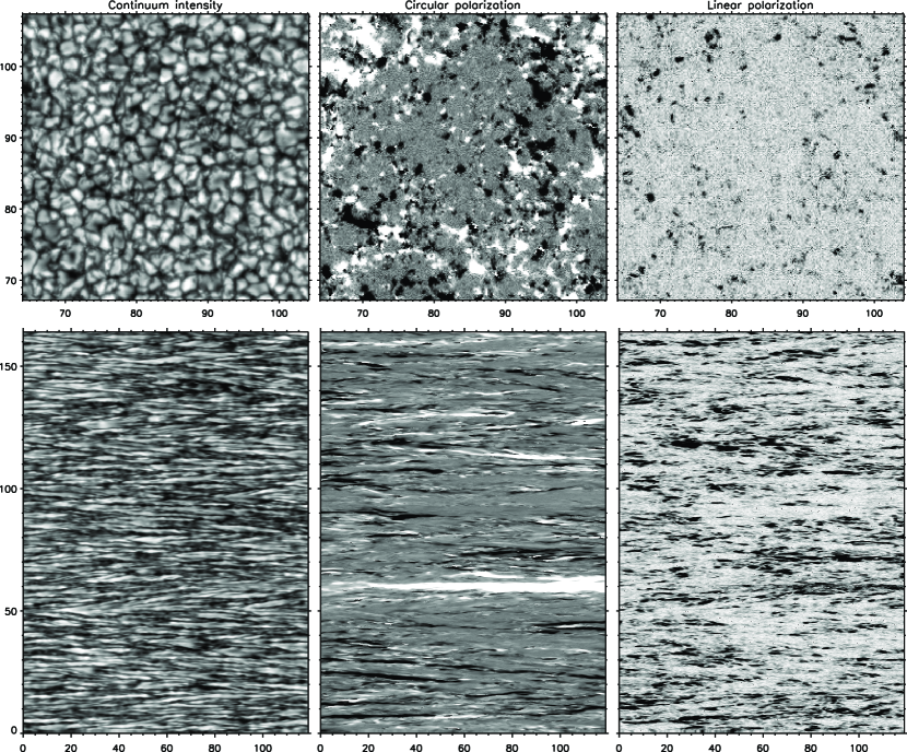
Figure 1.— Top: Small IN subfield of 40″$\times$40″ corresponding to data set #1. From left to right: continuum intensity, mean degree of circular polarization, and mean degree of linear polarization. The granulation contrast is 7.44%. This area contains a supergranular cell of about 30 000 km². Tickmarks are spaced by 1 arcsec. Bottom: Quiet Sun region covered by data set #2. The contrast is 7.3%. The x-axis represents time in minutes and the y-axis distance along the slit in arcsec. In both cases, the polarization maps have been computed as $[\sum_{i=N_{\rm b}}^{N_{\rm zc}}V(\lambda_{i})/I(\lambda_{i})-\sum_{i=N_{\rm zc}}^{N_{\rm r}}V(\lambda_{i})/I(\lambda_{i})]/(N_{\rm r}-N_{\rm b})$ and $\sum_{i=N_{\rm b}}^{N_{\rm r}}\sqrt{Q(\lambda_{i})^{2}+U(\lambda_{i})^{2}}/I(\lambda_{i})/(N_{\rm r}-N_{\rm b})$, respectively. $N_{\rm b}$ is the index where the Stokes V blue lobe of Fe I 630.25 nm starts, and $N_{\rm r}$ the index where the red lobe ends. $N_{\rm zc}$ represents the index of the Stokes V zero crossing. $N_{\rm r}-N_{\rm b}=22$ is the number of wavelength points used for the calculations. The circular and linear polarization maps are saturated at $\pm 0.15\%$ of the quiet Sun continuum intensity.

However, there still exists some skepticism about the accuracy of the magnetic parameters derived from ME inversions of the Hinode measurements (e.g., de Wijn et al. 2009; Bommier et al. 2009). Doubts affect particularly the distribution of field inclinations. Asensio Ramos (2009) and Borrero & Kobel (2011), using two different statistical analyses, recently pointed out that the information contained in the Stokes profiles is not enough to constrain the magnetic field inclination when the polarization signals are small and Stokes Q and U are buried in the noise. As a consequence, the true amount of inclined fields may not be recovered accurately without clear linear polarization signals. The model assumptions may also induce large uncertainties in the retrieved inclinations.

Always present in real observations, photon noise hides the weakest polarization signals and distorts the larger ones. There are two ways to partly circumvent this problem: to reduce the noise itself and/or to increase the signal. Both strategies lead to higher signal-to-noise ratios (S/N), allowing for a more precise discrimination between the magnetic field strength, field inclination, and filling factor in the quiet photosphere. The noise can be reduced by using larger telescopes or longer effective exposure times; the signals are enhanced by improving the spatial resolution, since this minimizes the cancellation of opposite-polarity fields.

Here we update our results from the inversion of Hinode/SP data (Orozco Suárez et al., 2007b, c; Orozco Suárez, 2008) by analyzing new measurements with significantly better S/N of up to 3500. In Section 2 we describe the observations, study the amplitudes of the observed polarization signals, and give an account of the Milne-Eddington inversion strategy we follow. In Section 3 the results of the inversion are presented. Section 4 discusses the effects of noise on the inferences, taking advantage of the availability of two data sets with different S/N. In Section 5 we determine very precise distributions of field strength and field inclination for pixels that show linear polarization signals well above the noise level. The magnetic flux density, the average field strength, and the vertical and horizontal components of the field are calculated and compared with previous observational determinations and magneto-convection simulations in Section 6. To highlight the distinct character of IN fields, Section 7 describes the magnetic properties of the network as deduced from the inversion. Finally, we discuss our results in Section 8.

2. Observations, noise analysis, and inversion of Stokes profiles

The observations analyzed in this paper come from two different data sets taken at disk center. Hereafter they will be referred to as normal map observations (set #1) and high S/N time series (set #2). Lites et al. (2007, 2008), Orozco Suárez et al. (2007b, c), Asensio Ramos (2009), Borrero & Kobel (2011), and Asensio Ramos & Manso Sainz (2011) have also used these measurements. Their main parameters are summarized in Table 1.

In observation #1, the spectrograph slit (of width 0.16″) was moved across the solar surface in steps of 0$\farcs$1476 to measure the four Stokes profiles of the Fe I 630 nm lines with a spectral sampling of 2.15 pm pixel^-1 and a exposure time of 4.8 s. For data set #2, the slit was kept fixed at the same spatial location and the Stokes spectra were recorded with an exposure time of 9.6 s. The completion of data set #1 took about 3 hours while the time series of data set #2 covers one hour and 51 minutes.

The effective exposure time of observation #2 was increased by averaging seven consecutive 9.6 s measurements. This allowed a final exposure time of 67.2 s to be reached, which corresponds to a S/N gain by a factor of about 3.8 with respect to data set #1. The averaging decreased the spatial resolution of the observations to some degree, but the granulation pattern is still perfectly visible due to the longer lifetime of photospheric convective structures (about 5 min, see Title & Schrijver 1998) and the excellent stabilization system of Hinode (Shimizu et al., 2008). Indeed, the rms continuum contrast of the granulation in the high S/N series is only 0.14% smaller than in the normal map. This variation is real, since the SOT focus position was optimized for the SP observations in the two cases.

Table 1Log of the observations

	Data set #1	Data set #2
	(Normal map)	(High S/N time series)
Date	2007 March 10	2007 February 27
Start time (UT)	11:37:37	00:20:00
FOV	302″$\times$162″	302″$\times$0$\farcs$16
(Pixels)	1024$\times$2048	1024$\times$727
Exposure time	4.8 s	67.2 s
Stokes V noise ($\sigma_{\rm V}$)	$1.1\times 10^{-3}\,I_{\rm QS}$	$2.9\times 10^{-4}\,I_{\rm QS}$
Stokes Q,U noise ($\sigma_{\rm Q,U}$)	$1.2\times 10^{-3}\,I_{\rm QS}$	$3\times 10^{-4}\,I_{\rm QS}$

The polarization noise levels ($\sigma$) are shown in Table 1. They were obtained as the mean value of the standard deviation of the corresponding Stokes signals in continuum wavelengths. Before evaluating the noise, the data were corrected for dark current, flat-field, and instrumental crosstalk. The whole process was accomplished using the routine sp_prep.pro included in SolarSoft. The Stokes profiles were normalized to the average quiet Sun continuum intensity, $I_{\rm QS}$, computed using all pixels from each data set.

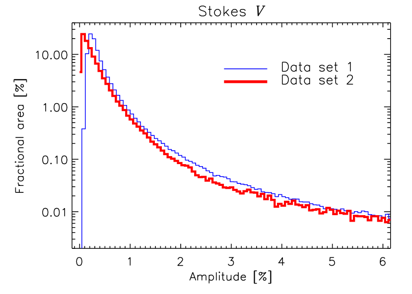
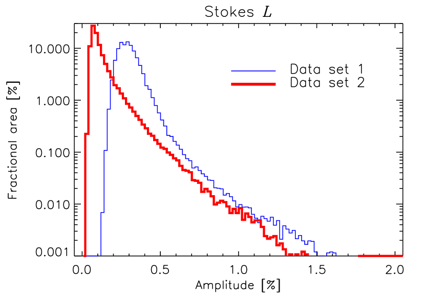
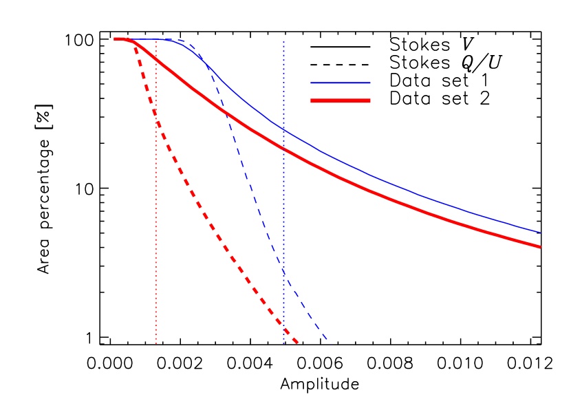
Figure 2.— Top: Amplitudes of the observed Stokes V profiles, in units of $I_{\rm QS}$. The thin and thick lines indicate the normal map and the high S/N time series, respectively. Middle: Same, for Stokes Q and U (the one with the largest amplitude is selected). Bottom: Surface area occupied by signals with Stokes V or Stokes Q or U amplitudes larger than a given value. Vertical lines mark the 4.5$\sigma$ noise thresholds for the two data sets analyzed in this paper.

Figure 1 displays maps of the continuum intensity and mean circular and linear polarization degrees for data sets #1 and #2. The different nature of the two observations is apparent. The normal map, as a “snapshot” of the solar surface, reveals the spatial distribution of convective cells and magnetic flux concentrations in the quiet Sun. By contrast, data set #2 shows the evolution of these structures. For instance, granules (intergranules) are seen as bright (dark) horizontal streaks. Flux concentrations also produce horizontal streaks which last longer in circular polarization. Note that data set #2 exhibits many more linear polarization patches than the normal map because of the lower noise level.

Figure 2 shows histograms of the circular (Stokes V) and linear (Q, U) polarization amplitudes of Fe I 630.25 nm (top and middle panels, respectively) in the two data sets. They demonstrate the large occurrence of weak polarization signals. The distributions are similar for the high S/N time series and the normal map, although some differences exist. For example, the normal map histograms peak at larger amplitudes. In both data sets, however, the peaks are close to the corresponding noise levels: the Stokes V distributions reach their maxima at about 1.95$\sigma_{\rm V}$ and 2.35$\sigma_{\rm V}$, respectively, while the linear polarization histograms peak at 2.42$\sigma_{\rm Q,U}$ and 2.33$\sigma_{\rm Q,U}$.

To avoid polarization signals that are highly contaminated by noise, we only consider pixels with Stokes Q, U or V amplitudes larger than 4.5$\sigma_{\rm V}$. This criterion is very restrictive: the probability that one pixel showing pure noise in all three Stokes parameters be included in the analysis because one of the signals exceed by chance the 4.5$\sigma_{\rm V}$ level is only 0.19%. This number results from the multiplication of three factors: the probability of $7\times 10^{-6}$ that a single measurement of a zero signal exceeds $\pm 4.5\sigma_{\rm V}$ when the noise follows a normal distribution, the three Stokes parameters that we consider, and the 90 wavelength points used to compute the amplitude of the polarization signals. With such a low probability, we can be sure that the inverted profiles are real and not due to noise.

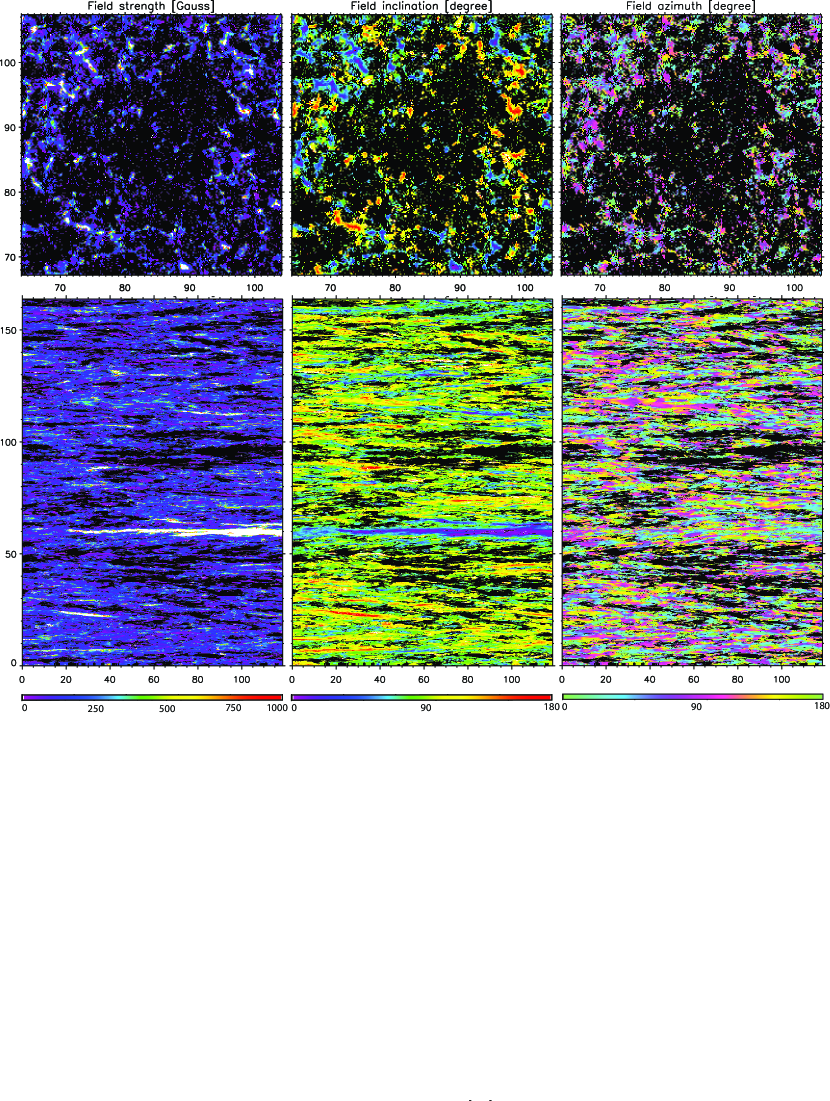
Figure 3.— Magnetic field parameters resulting from the inversion of the normal map (top row) and the high S/N time series (bottom row). Shown from left to right are magnetic field strengths, inclinations, and azimuths. Pixels in black did not meet the selection criterion and were not inverted. The field strength map is saturated at 1 kG so the pixels in white correspond to fields $\geq$ 1 kG. The FOVs are the same as in Figure 1. Tickmarks are spaced by 1 arcsec in the normal map. In the high S/N time series the x-axis represents time in minutes and the y-axis distance along the slit in arcsec.

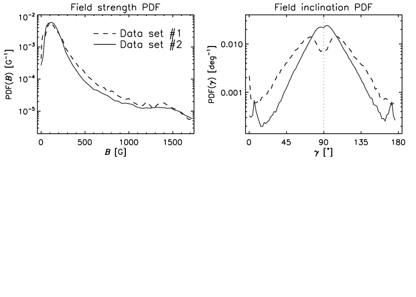
Figure 4.— Magnetic field strength (left) and inclination (right) probability density functions for IN regions resulting from the inversion of data sets #1 and #2 (dashed and solid lines, respectively). The PDF for the magnetic field strength corresponding to data set #2 resamples quite well the one corresponding to the normal map, despite the very different S/N. These PDFs are derived from the analysis of pixels with Stokes Q, U or V amplitudes larger than 4.5 times the noise level. The fraction of the FOV they cover is 26.8% in the normal map and 72.7% in the high S/N time series. Of these pixels, 7.9% and 37.7% show linear polarization signals above 4.5$\sigma_{\rm Q,U}$.

The bottom panel of Figure 2 shows the fraction of the FOV with Stokes V signals above a given amplitude. A similar curve is provided for the linear polarization signals (Stokes Q or U). The vertical lines indicate 4.5 times the noise level in Stokes V for data sets #1 and #2. Only 26.0% of the normal map area exhibit Stokes V amplitudes above our $4.5\sigma_{\rm V}$ noise threshold. This fraction increases to 70.1% in the high S/N time series. The area with Stokes Q or U signals larger than 4.5$\sigma_{\rm Q,U}$ is smaller, only 2.1% and 27.4%, respectively. In summary, the fraction of pixels fulfilling the selection criterion (i.e., Stokes Q, U, or V amplitudes larger than 4.5 times their noise levels) is 26.8% and 72.7% in data sets #1 and #2 (corresponding to about 0.7 and 1.6 Mpx). For comparison, 62.6% and 85.7% of the FOV covered by the two observations show Stokes V signals above $3\sigma_{\rm V}$ (cf. the 92.6% of Martínez González et al. 2008 and the 80-90% reported by Khomenko et al. 2005, both from ground-based observations).

In the normal map the selection of IN areas has been done manually to avoid the strong flux concentrations of the network (see Orozco Suárez 2008 for details). In the high S/N time series we have just removed the strong magnetic feature of positive polarity visible at around 1/3rd of the slit ($y=60$″).

The observations are analyzed using least-squares inversions based on a one-component, horizontally homogeneous ME atmosphere, as described by Orozco Suárez et al. (2007a, b, c). We include a local non-magnetic component to account for the reduction of the polarization signals induced by the instrument’s Point Spread Function (PSF). This component was called “local” stray-light contamination in Orozco Suárez et al. (2007a). Here we use a different name to better reflect the nature of this contribution and distinguish it from real stray light, i.e., light that enters the detector because of unwanted reflections in the mirror surfaces, supporting structures, etc. For the normal map, the local non-magnetic contribution is evaluated by averaging the Stokes I profile within a 1″-wide box centered on the pixel. For the high S/N time series we take the non-magnetic component as the average Stokes I profile along 1″ of the SP slit centered on the pixel. The reason is that we cannot perform a two-dimensional average since the data is one-dimensional. With this approximation we avoid using measurements acquired more than a minute apart, although the non-magnetic profile may not appropriately account for the effects of the PSF. Further information about how the PSF changes the polarization signals are given in Orozco Suárez et al. (2007a) and del Toro Iniesta & Orozco Suárez (2010). The implications of using a local stray light have been analyzed by Asensio Ramos & Manso Sainz (2011). In practice, our approach is equivalent to a two-component inversion in which the non-magnetic atmosphere has only one free parameter, $(1-f)$, with $f$ the magnetic filling factor. The two Fe I lines were inverted simultaneously with the MILOS code (Orozco Suárez & Del Toro Iniesta, 2007; Orozco Suárez et al., 2010a). The use of two lines, as opposed to only one (e.g., Bommier et al. 2009), reduces the influence of noise and leads to more accurate results (Orozco Suárez et al., 2010a).

3. Inversion results

Maps of the field strengths, inclinations, and azimuths retrieved from the two data sets are shown in Figure 3 (see also Orozco Suárez et al. 2007b, c and Orozco Suárez 2008). Pixels in black were not inverted because their Stokes Q, U, or V amplitudes do not exceed 4.5$\sigma_{\rm V}$. Qualitatively, the inversions of the two data sets give the same results. Most of the fields are weak (of the order of hG), with the stronger field concentrations located in intergranular lanes. The fields are very inclined, especially in granules. The azimuth is much better recovered in the high S/N time series due to the lower noise of the linear polarization profiles.

Figure 4 shows the probability density function (PDF; Steiner 2003) of magnetic field strengths and field inclinations in the IN for the normal map and the high S/N time series (dashed and solid lines, respectively). We recall that they were obtained from the analysis of Stokes profiles whose amplitudes exceed a polarization threshold of $4.5\sigma_{\rm V}$. The S/N of data set #2 is about 3.8 times better than that of the normal map. However, the peaks of the field strength distributions are located at nearly the same position ($\sim$ 90 G) and have very similar widths. A closer inspection shows that the maximum of the field strength distribution for the high S/N time series occurs at around 100 G, i.e., at slightly stronger fields. These PDFs seem to indicate that the IN consists of hG flux concentrations. In general, the field strength PDF does not change when using better S/N data, suggesting that the inversion results are reliable and not affected by the noise of the profiles.

The inclination PDF for the normal map has a maximum at 90^∘ and decreases toward vertical orientations. Near 0^∘ and 180^∘ the PDF increases again. The distribution of field inclinations derived from the high S/N data is very similar, with some minor differences: first, the amount of nearly horizontal fields increases with respect to that in the normal map, indicating that the smallest polarization signals (not considered before) are also associated with highly inclined fields; second, the PDF is narrower, so that the fields are less abundant as they become more vertical. Overall, the two distributions point to large IN field inclinations.

4. Reliability of the inferred magnetic field distributions

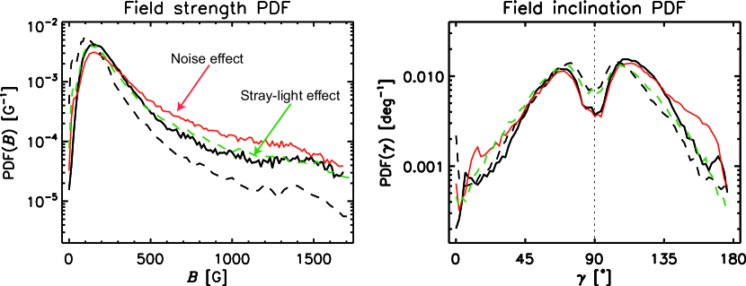
Figure 5.— Magnetic field strength (left) and field inclination (right) distributions for IN regions of data sets #1 and #2 (dashed and solid lines, respectively). They have been determined from pixels whose Stokes Q, U or V amplitudes exceed the same absolute threshold of 0.5% the quiet Sun continuum intensity (black curves). For the normal map, this amplitude represents $4.5\sigma_{\rm V}$ (and the corresponding PDFs are identical to those displayed in Figure 4). For the high S/N data, an amplitude of $0.5\%\,I_{\rm QS}$ is 16.4 times larger than the noise. The percentage of pixels fulfilling the selection criterion is 26.8% in the normal map and 16.4% in the high S/N data. Of these pixels, 7.9% and 6.8% show linear polarization signals above the noise threshold, respectively. The solid red lines stand for the inversion of the same high S/N profiles once their noise has been artificially increased to a level comparable to that found in data set #1. The percentage of analyzed pixels is then 16.4%, of which 6.8% show linear polarization signals above 0.5% I_QS. Finally, thegreen lines represent the results of the inversion of data set #1 calculating the non-magnetic component as in data set #2.

The polarization signals we measure in the internetwork are tiny compared to those found in active regions. As a consequence, a careful treatment of the noise is important to interpret them correctly. The first obvious choice to minimize the effects of noise was to set a rather conservative threshold on the amplitude of the polarization signals, which had to exceed 4.5 times the noise level to be included in the analysis. We used this criterion to identify and avoid the noisier signals that cannot be inverted reliably.

The threshold of $4.5\sigma_{\rm V}$ was chosen taking into consideration the results presented by Orozco Suárez et al. (2007a) and Orozco Suárez (2008). There, Hinode/SP normal map observations were simulated with the help of 3D magnetoconvection models to determine whether it is possible to recover the distribution of magnetic field strengths and inclinations with a S/N of 1000 and a threshold of $4.5\sigma_{\rm V}$. The results showed that the field strength and the field inclination can be recovered with mean errors of less than 100 G and 10^∘, respectively. For very weak fields ($B\sim 100$ G), the rms uncertainty of the inclination is smaller that 30^∘, sufficient to distinguish between highly inclined and vertical fields. The errors in field strength and inclination are expected to be smaller for measurements with lower noise levels, such as the high S/N time series.

However, the influence of noise is still of concern. Asensio Ramos (2009) analyzed a small region of the normal map using Bayesian techniques and Milne-Eddington inversions. His results suggest that while the magnetic field strength tends to be well recovered, it is in general not possible to constrain the field inclination when the signals are very weak and Stokes Q or U do not stand out prominently above the noise. A possible consequence of the limited information carried by the Stokes vector when Q and U are buried in the noise is an overabundance of horizontal fields. This is because inversion algorithms try to fit the noise of the linear polarization profiles (Khomenko et al., 2003).

Also Borrero & Kobel (2011) have recently argued that the noise present in Stokes Q and U can potentially distort the Milne-Eddington inferences. These authors showed how in some cases inclined fields may be obtained from purely vertical weak magnetic fields. This happens when the noise in Stokes Q and U is interpreted as a real signal. In the weak field regime, producing linear polarization in Fe I 630 nm at the level of the noise requires large transverse fields. Thus, the noise may be compatible with highly inclined fields. An additional effect is that the recovered fields are stronger than the real ones. Borrero & Kobel (2011) inverted the two data sets used in this paper (but only one spectral line, not the two) and detected a small shift of the peak of the field strength PDF toward weaker fields for the data with better S/N, which they interpreted as evidence that noise was playing an important role.

There are reasons to believe that the field strength and field inclination distributions we have derived are reliable and not significantly affected by the noise, even if most of the pixels do not show significant Stokes Q or U signals. The following arguments support this conclusion:

• If noise were affecting the inversions, the fields obtained from the normal map (the noisier one) would be stronger and more inclined than those from the high S/N data, as claimed by Borrero & Kobel (2011). Our distributions indeed show a small shift when the S/N is improved, but in the opposite direction, i.e., toward stronger fields (see Figure 4).

• Although only 27.4% of the pixels in the high S/N time series have linear polarization signals above $4.5\sigma_{\rm Q,U}$, the maps of magnetic field inclination and particularly the azimuth derived from the inversion are dominated by structures which vary smoothly both in time and in space (Figure 3). These structures are real and not caused by the noise. Therefore, the smallest linear polarization signals below $4.5\sigma_{\rm Q,U}$ also provide information to constrain the field azimuth and inclination.

• In the absence of clear Stokes Q and U signals it may still be possible to gather information about the field inclination: first, the noise in Q and U sets limits on it, and second, in the weak field regime Stokes I has greater sensitivity to the inclination than Stokes Q, U, or V (del Toro Iniesta & Orozco Suárez, 2010).

At this point, a solid demonstration that noise is not affecting the determination of field strengths and inclinations would come from the similarity of the results derived from pixels which show the same type of polarization signals but have very different noise levels. Thus, in Figure 5 we compare the PDFs calculated from pixels with Stokes Q, U, or V signals larger than 0.5% I_QS in both data sets. For the normal map (black dashed line), this amplitude threshold represents 4.5 times the noise level, but for the high S/N observations (black solid line) the same absolute threshold corresponds to signals 16 times larger than the noise. Unexpectedly, we observe some differences in the shapes of the resulting PDFs. For example, the peak of the field strength distribution obtained from the high S/N measurements is slightly shifted toward stronger fields compared to the normal map. This implies a smaller abundance of weak fields and a larger fraction of strong fields. Also, the two inclination PDFs show a dip at around 90^∘, but less pronounced in the case of the high S/N measurements.

These differences may reflect a better determination of the magnetic field parameters from the less noisy signals. Alternatively, they may indicate intrinsic differences between the two data sets or problems with the inversion scheme. To identify the actual origin of the differences, we have carried out two additional tests. In the first one, we have artificially increased the noise of data set #2 to the level of the normal map. Then we have inverted the pixels with Stokes Q, U, or V signals above 4.5 times the new noise level. Since this sample of profiles has the same noise as data set #1, one should expect PDFs similar to those obtained from the normal map (black dashed line in Figure 5). The differences between the new PDFs and the black solid lines should only be ascribed to the increased noise. The outcome of this exercise is shown in Figure 5 with red solid lines. As can be seen, the new PDFs are closer to the ones derived from the high S/N measurements (black solid line) than to the normal map PDFs. Compared with the original high S/N measurements, the abundance of weak fields ($0<B<300$ G) decreases and the fraction of strong fields ($B>300$ G) increases, but the peak of the PDF remains at the same position. The fraction of inclined fields is also very similar, with slightly less vertical fields. These results indicate that noise is not producing the differences between the black curves of Figure 5, since the inversion of data set #2 with enhanced noise does not reproduce the normal map PDFs. Thus, the cause of the differences must be found elsewhere. Another interesting result is the following. From the comparison of the PDFs derived from data set #2 with varying noise levels (black and red solid curves), we do not confirm the conclusion of Borrero & Kobel (2011) that an increase of the noise in Stokes Q and U shifts the PDFs to stronger and more horizontal fields. The red curves, much more affected by noise than the black curves but otherwise coming from exactly the same profiles, do not show any of the two effects. This is probably due to the fact that we analyze real observations where the fields are not completely vertical, contrary to the situation modeled by Borrero & Kobel (2011).

In the second test we examine the influence of the local non-magnetic contribution, which is calculated differently in the two data sets. To that end, we have repeated the inversion of the normal map using a non-magnetic contribution obtained as in the case of the high S/N time series, i.e., by averaging the Stokes I profiles over 1″ along the slit. The results, depicted in Figure 5 with green dashed lines, show that the fraction of weak fields (below 300 G) decreases and the amount of strong fields increases with respect to the dashed black curves. The PDF peak shifts to stronger fields. Remarkably, the field strength PDF coincides with that calculated from the pixels in the high S/N time series that show Stokes Q, U, or V amplitudes larger than 0.5% I_QS. The inclination PDF does not change much. Overall, this test suggests that (part of) the differences between the normal map and the high S/N time series observed in Figure 5 may be the result of the different treatment of the non-magnetic component in the two data sets.

5. Analysis based on linear polarization signals

Figure 6.— Observed (dots) and best-fit (solid) Stokes profiles corresponding to a pixel with linear polarization signals above 4.5 times the noise level. The field strength, inclination, azimuth, and filling factor retrieved for this pixel are 193 G, 104^∘, 76 ^∘, and 33%. The horizontal lines mark the 4.5$\sigma$ threshold.

To obtain the most accurate results, in the rest of the paper we will focus on the analysis of pixels from the high S/N time series showing Stokes Q or U signals above $4.5\sigma_{\rm Q,U}$. With Q and U clearly above the noise, a very precise determination of the field inclination can be made because the inversion code uses the maximum amount of information possible (Asensio Ramos, 2009; Borrero & Kobel, 2011). The field strength is also obtained more accurately, due to the different dependence of the linear and circular polarization on B in the weak field regime.

To illustrate how these signals look like, Figure 6 shows the Stokes profiles of a typical IN pixel whose linear polarization is just above the 4.5$\sigma_{\rm Q,U}$ level. We also include the corresponding best-fit profiles. The fit is quite successful even though the signal is close to the threshold and Stokes V is slightly asymmetric. Note that the linear polarization signals are above the noise threshold (horizontal lines) at several wavelength positions, not just one, which allows the inversion code to determine the field inclination and the azimuth accurately because the whole polarization profiles are recognizable. In this case, the inversion returns a field strength of 193 G, an inclination of 104^∘, an azimuth of 76^∘, and a filling factor of 33%.

Figure 7.— High-precision magnetic field strength and inclination distributions for IN regions derived from data set #2. The PDFs are based on the inversion of pixels whose Stokes Q or U amplitudes exceed 4.5$\sigma_{\rm Q,U}$. They represent 27.4% of the surface area covered by the IN. About 90.3% of those pixels show circular polarization signals above the noise threshold.

An analysis restricted to pixels showing linear polarization signals is very reliable because the effects of noise are largely suppressed. However, the price to pay is a reduced coverage of the internetwork (only 27.4% of the IN surface area) and a bias towards inclined and/or strong fields, since those are the fields that more easily produce linear polarization signals. We do not know exactly the amount of bias, but this possibility should be kept in mind. In any case, the data we are considering represent more than 1/4th of the internetwork, which is non negligible. Of all the pixels selected for analysis, 90.3% also show Stokes V amplitudes above $4.5\sigma_{\rm V}$.

Figure 7 shows our most precise determination of the field strength and field inclination distributions in the IN based on pixels of the high S/N time series with Stokes Q or U amplitudes exceeding $4.5\sigma_{\rm Q,U}$. These PDFs confirm the main results derived from the analysis of all the pixels that met the inversion threshold, namely that the IN fields are weak and very inclined. It is remarkable that the maximum of the field strength PDF remains at more or less the same position, with only a small shift toward stronger fields (about 130 G). The inclination PDF is narrower than the ones displayed in Figure 4. Very likely, this is due to selection effects: the more vertical fields are excluded from the analysis because they produce smaller Stokes Q and U signals. Therefore, the amount of vertical fields can be expected to decrease with respect to that found when analyzing pixels with Q, U, or V above 4.5 times the noise level.

Figure  8 shows the filling factors inferred from the inversion of the profiles in the high S/N time series with Q or U signals above 4.5 times the noise level. As can be seen, the maximum of the distribution occurs at around 0.25, with a tail extending toward filling factors of up to 0.4–0.6. Such values are significantly larger than those obtained from ground-based observations, and imply that some of the IN fields are almost resolved by the Hinode SP. This seems plausible in view of the recent detection of resolved network flux tubes by Lagg et al. (2010), using data taken with the IMaX magnetograph (Martínez Pillet et al., 2011) aboard the SUNRISE balloon-borne solar observatory (Solanki et al., 2010). The resolution of the IMaX measurements is 0$\farcs$18, nearly twice as good as that provided by the Hinode SP.

Figure 8.— Distribution of magnetic filling factors retrieved from the inversion of the high S/N time series including only pixels whose Stokes Q or U amplitudes exceed 4.5$\sigma_{\rm Q,U}$ (solid). For comparison, we also represent the distribution corresponding to all pixels whose Stokes Q, U, or V amplitudes exceed 4.5$\sigma_{\rm V}$ (dashed).

6. Average magnetic parameters in the quiet Sun

Figure 9.— Distribution of magnetic field strength (left) and inclination (right) in network regions resulting from the inversion of data set #1. The solid lines stand for all pixels within the selected network areas and the dashed lines for pixels associated with network flux tubes (see text).

6.1. The average field strengths

We calculated the mean magnetic field strength, $\langle B\rangle=\sum_{i=1}^{N}B_{i}/N$, and the mean vertical and horizontal components of the field, $\langle B_{\rm z}\rangle=\sum_{i=1}^{N}|B_{{\rm z},i}|/N=\sum_{i=1}^{N}|B_{i}\cos\gamma|/N$ and $\langle B_{\rm h}\rangle=\sum_{i=1}^{N}(B_{{\rm x},i}^{2}+B_{{\rm y},i}^{2})^{1/2}/N=\sum_{i=1}^{N}|B_{i}\sin\gamma|/N$, where $N$ is the number of pixels, using the results from the analysis of the pixels with Stokes Q or U signals above $4.5\sigma_{\rm Q,U}$ in the high S/N time series. The values of $\langle B\rangle$, $\langle B_{\rm z}\rangle$, and $\langle B_{\rm h}\rangle$ we obtain are 220, 64, and 198 G, respectively. The dominance of $\langle B_{\rm h}\rangle$ over $\langle B_{\rm z}\rangle$ indicates that the fields are highly inclined in the IN, as first pointed out by Lites et al. (2007, 2008). Since in the rest of pixels the linear polarization signal does not surpass the noise threshold, they likely have weaker fields. For that reason, the above values can be interpreted as upper limits for the mean field strength in the internetwork. Note that the quantities $\langle B\rangle$, $\langle B_{\rm z}\rangle$ and $\langle B_{\rm h}\rangle$ are independent of the magnetic filling factor.

The ratio between the horizontal and vertical components of the field in IN regions is $r\sim 3.1$ according to our results. Lites et al. (2007, 2008) estimated a larger ratio $r\sim 5$ for all pixels within the field of view, but this value cannot be directly compared to ours because it is based on “apparent” magnetic flux densities rather than on intrinsic field strengths. In addition, the method of Lites et al. (2007, 2008) uses less information than Stokes inversions (for instance, Stokes I was not considered) and might be affected by noise differently.

Our results partially agree with the MHD simulations of Steiner et al. (2008), in which the magnetic field dynamics is mainly driven by flux expulsion and overshooting convection. Steiner et al. (2008) computed the horizontally and temporally averaged absolute vertical and horizontal magnetic field components as functions of height for two different simulation runs and found a maximum horizontal/vertical field component ratio of about 2.5 at 500 km (see Figure 1 in their paper). This is comparable with the value we have obtained from the inversions. However, the average horizontal and vertical magnetic field strengths they find are still smaller than ours.

Recently, Danilovic et al. (2010) have presented a set of local dynamo simulations and have compared them with the results of Lites et al. (2007, 2008) (see also Bello González et al. 2009 for a comparison between ground-based observations and simulations). Following a similar approach as Steiner et al. (2008), these authors synthesized the Stokes profiles of the 630 nm lines from the simulated models and degraded them to the resolution of the Hinode SP (Danilovic et al., 2008). After adding noise, they calculated the longitudinal and transverse apparent flux densities. Their results suggest that current local dynamo simulations explain the value of $r\sim 5$ obtained by Lites et al. (2007, 2008). However, to reproduce the amount of transverse and longitudinal flux and the variation of the flux ratio with heliocentric angle, Danilovic et al. (2010) had to artificially increase the average magnetic field strength in the simulation by a factor of 2 or 3, depending on the dynamo run. With a factor of 3, their average field turns out to be about 170 G at $\log\tau=0$, in agreement with Hanle measurements (Trujillo Bueno et al., 2004). This prompted Danilovic et al. (2010) to argue that current Hinode observations can be well explained by local dynamo processes.

The local dynamo simulations with artificially increased fields are roughly compatible with our results. The average field strength of 170 G worked out by Danilovic et al. (2010) is below the upper limit of 220 G we have deduced. In their simulations the vertical and horizontal components of the field are also smaller than those reported in this work. Finally, the ratio of horizontal to vertical field components varies between 2 and 4 in the range $-2<\log\tau<-1$ (cf. Schüssler & Vögler 2008), which is compatible with our value $r\sim 3.1$

The two mechanisms put forward to explain the existence of very inclined fields in the IN, namely convective overshoot (Steiner et al., 2008) and local dynamo action (Danilovic et al., 2010), may operate simultaneously or may not occur in the real Sun. To distinguish between the different possibilities it is necessary to perform detailed comparisons of the magnetic field distributions predicted by the simulations and those obtained from the observations. This would give much more information than just a single parameter such as the ratio of horizontal to vertical magnetic field components.

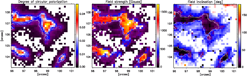
Figure 10.— Small area of about 5″$\times$5″ showing the degree of circular polarization (left), the field strength (middle) and the field inclination (right) resulting from the inversion of normal map data. This area contains several network elements. The white pixels were not inverted. Contour lines enclose areas with field strengths greater than 700 G (dotted), inclinations lower than $25^{\circ}\/$ (solid), and polarization signal amplitudes above $2\times 10^{-2}\,I_{\rm QS}$ (dashed).

6.2. The average magnetic flux density

The determination of the average flux density of IN regions has been pursued for many years, which has resulted in more than forty papers to date. Unfortunately, there is a large disparity between the values obtained by the different authors. One of the reason is that the estimates are strongly affected by the angular resolution of the observations. Also the different analysis techniques have contributed to the discrepancies. As a result, the flux values reported in the literature vary from the 2–3 Mx cm^-2 of, e.g., Lin & Rimmele (1999) and Keller et al. (1994), to the 15–20 Mx cm^-2 found by Domínguez Cerdeña, (2003), Viticchié & Sánchez Almeida (2011), Beck & Rezaei (2009), and Bello González & Kneer (2008). Studies using simultaneous observations of visible and infrared lines give 11–15 Mx cm^-2 (Khomenko et al., 2005). An upper limit to the flux density seems to be $\sim$ 50 Mx cm^-2 (e.g., Faurobert et al. 2001).

We have calculated the average magnetic flux density $\langle\phi\rangle=\sum_{i=1}^{N}|\phi_{i}|/N$ using the parameters retrieved from the inversion of the high S/N time series. The flux of individual pixels is computed as $\phi=fB\cos\gamma$. Note that, as opposed to the magnetic field strength $B$, the flux density depends on the magnetic filling factor. The average is carried out in two different ways: taking into account only those pixels with Stokes Q or U amplitudes above 4.5 $\sigma_{\rm Q,U}$ and considering all pixels. In the latter case, the average flux represents a lower limit because we assign zero fluxes to pixels without clear linear polarization signals (even if they show large Stokes V amplitudes).

We find a flux density of 16.3 Mx cm^-2 in the 27.4% of the FOV with significant linear polarization signals. A lower limit for the flux, considering all pixels, is 4.5 Mx cm^-2. These results agree with the latest estimations of 11–16 Mx cm^-2 by Lites (2011). Our flux densities are slight smaller than those derived recently from the analysis of near infrared lines by Beck & Rezaei (2009), who found fluxes of about 26 G and a lower limit of 22 G. They are also smaller than the ones obtained from observations in the visible with the GREGOR Fabry-Perot spectrometer attached to the German Vacuum Tower Telescope: according to Bello González & Kneer (2008), a lower limit for the flux would be 17 G. Finally, the net flux density, calculated as $\langle\phi\rangle_{\mathrm{n}}=\sum_{i=1}^{N}\phi_{i}/N$, amounts to $-2.9$ Mx cm^-2.

7. Differences with the network

In this Section we show that the properties of network and internetwork fields are rather different, as expected from their different nature. The distribution of network field strengths and inclinations obtained from the analysis of the normal map can be seen in Figure 9. The PDF for the field strength (solid line) peaks at $\sim$ 100 G but has a prominent hump centered at about 1.4 kG, in contrast to what is found in the IN where the majority of fields are in the hG range (Figure 7). In the same figure we give the distribution of fields for the inner pixels of the network flux concentrations (dashed line). They are selected by their circular polarization amplitudes, which have to be larger than 0.03 I_QS. For those pixels, the peak at 100 G shifts toward stronger fields and becomes smaller than the hump at 1.4 kG. The PDF vanishes very rapidly below 300 G.

The inclination PDF corresponding to the network areas (solid line) is dominated by inclined fields, but has secondary peaks at $\sim$ 10^∘ and 170^∘. The slightly asymmetric shape of the distribution is due to the predominance of positive polarities among the network areas selected for analysis. When we consider only the stronger network concentrations (dashed line), the peaks at 10^∘ and 170^∘ become dominant and the inclined fields disappear.

The network PDFs show what is expected from intense field concentrations, i.e., kG fields with predominantly vertical orientations. The field strength and field inclination peaks we observe are compatible with the results of analyses at lower spatial resolution (e.g., Solanki et al. 1987 and Sánchez Almeida & Martínez Pillet 1994). The large fraction of inclined fields as well as the tail and hump of the field strength distribution toward weak fields represent the contribution of network canopies to the PDFs. Network canopies (see e.g. Pietarila et al. 2010 and references therein) are associated with more inclined and weaker fields and can be observed at the vicinity of strong network flux concentrations. To illustrate this, Figure 10 displays the magnetic field strength and inclination inferred from the ME inversion of a small area in data set #1 that includes network elements. Note that pixels corresponding to the innermost part of the network elements show strong vertical fields, while those at the periphery (canopy areas) are associated with weak fields and moderate-to-large inclinations.

8. Discussion and conclusions

In this paper we have carried out a Milne-Eddington analysis of high spatial resolution measurements of the quiet Sun taken with the Hinode spectropolarimeter. To infer the magnetic field vector we have applied the inversion strategy described by Orozco Suárez et al. (2007a) to two observations with different noise levels: $1.2\times 10^{-3}$ and $3\times 10^{-4}\,I_{\rm QS}$.

The magnetic field distributions obtained from the two data sets are rather similar, suggesting that they are not biased by photon noise. A more detailed analysis reveals that differences exist between the distributions when we consider the same type of polarization signals (Stokes Q, U, or V larger than 0.5% I_QS) but different noise levels. We performed two tests to assess how the noise and the calculation of the non-magnetic component affect the inversion results. We reach the conclusion that noise is of little concern. Rather, the results may be influenced by the different method we use to obtain the non-magnetic component in the two data sets. This test suggest that the field strengths may be slightly over-estimated in the high S/N data. The field inclinations do not seem to depend on the exact way the non-magnetic component is calculated.

We also provide magnetic field distributions in the IN based only on pixels that show significant linear polarization signals (Figure 7). Most of them also have large circular polarization signals. By restricting the analysis to those pixels we make sure that the inversion results are accurate. The downside is that they represent only 27.4% of the surface area covered by the IN. Our choice also implies that these high-precision magnetic field distributions may be biased toward stronger and/or more inclined fields—the ones that produce the larger linear polarization signals. A better coverage of the IN requires more sensitive measurements that are not yet available.

Keeping in mind these considerations, we discuss the main results of our analysis in the following subsections.

8.1. Internetwork fields are weak

The inversion of Hinode/SP data presented here indicates that IN fields are weak, at least in the 27.4% of the FOV showing Stokes Q or U signals well above the noise. This is in qualitative agreement with the picture derived from the more magnetically sensitive Fe I lines at 1565 nm (Lin, 1995; Lin & Rimmele, 1999; Collados, 2001; Khomenko et al., 2003; Domínguez Cerdeña et al., 2006; Beck & Rezaei, 2009) and with the simultaneous inversion of the Fe I 630 nm and 1565 nm lines performed by Martínez González et al. (2008). Also Rezaei et al. (2007) and Beck & Rezaei (2009) found weak fields in the IN from the analysis of Fe I 630 nm observations taken with the Polarimetric Littrow Spectrograph (Schmidt et al., 2003; Beck et al., 2005) at the German Vacuum Tower Telescope in Tenerife. Our findings are compatible with the results obtained by Asensio Ramos (2009) from the same data using Milne-Eddington inversions.

There are other measurements that point to the existence of weak fields in the IN. For example, the Mn I 553 nm line analyzed by López Ariste et al. (2006) suggests that the IN is dominated by fields below 600 G. Using the Mn I line at 1526.2 nm, Asensio Ramos et al. (2007) found a Gaussian-shaped distribution of field strengths centered at around 250-350 G. The manganese lines are important because the hyperfine effects they show make it possible to derive the strength of the field directly from the shape of the profiles. Since the polarization amplitudes are not used, the inferred field strengths are free from errors due to uncertainties in the actual stray-light contamination or in the magnetic filling factor.

The field strength PDF displayed in Figure 7 is not monotonic and has a clear maximum in the region of weak fields. Although the exact location of this maximum is still under debate, the peak itself is most probably solar in origin. Several authors have argued that peaks may result from the cancellation of magnetic flux at sub-resolution scales (e.g., Martínez González et al. 2008), but we do not favor this interpretation because our spatial resolution is much better than that of any previous measurement, which decreases the possibility of cancellations. This does not mean that cancellations do not exist at 0$\farcs$3, but that they are less frequent.

An important question is whether we should have considered more complex magnetic topologies than those allowed by the Milne-Eddington approximation. Viticchié et al. (2011) have recently analyzed Hinode/SP data assuming that the magnetic fields of the IN are small fibrils with sizes below $\sim$ 100 km, the mean photon free path in the solar photosphere. More specifically, they used a Micro-Structured Magnetic Atmosphere (MISMA) of the type described by Sánchez Almeida et al. (1996). With this model, Viticchié et al. (2011) were able to fit the asymmetries of the Stokes profiles recorded by Hinode (Viticchié & Sánchez Almeida, 2011). They found that a broad range of field strengths (from hG to kG) are present in IN regions. In particular, kG fields would dominate deep photospheric layers and hG fields the layers above. They argued that an IN consisting of fibrils with kG fields is partly compatible with the field strength PDFs shown in Figure 4, because the ME inferences carry information from high photospheric layers. However, we doubt that our findings and their results are truly compatible. First, the ME inferences cannot be assigned to specific atmospheric layers but rather provide average values over the region of formation of the spectral lines. Therefore, our field strength distributions should be similar to the ones they obtain, which is not the case. Second, the inversions performed by Viticchié et al. (2011) are very dependent on the assumptions of the MISMA model. In the absence of compelling proofs that the quiet Sun IN consists of small-scale, mixed-polarity magnetic fibrils that are still not resolved by Hinode, we tend to prefer more simplistic approaches like the Milne-Eddington inversions described in this paper.

Finally, we point out that our results seem to agree with those of Stenflo (2010). He reported the existence of two kinds of magnetic structures in the quiet Sun, one characterized by strong and vertical fields, and another by weak and isotropic fields. We believe that the strong fields are associated with the network elements, while the weak ones are those found in the IN, although Stenflo (2010) cautioned that the association of IN fields with the weak fields is not completely clear.

Figure 11.— Magnetic field inclination PDF of IN regions in the high S/N time series where the linear or circular polarization signals are larger than $1.35\times 10^{-3}$ I_QS (corresponding to $4.5\sigma_{\rm V}$, solid line) and pixels where the linear polarization exceeds the same threshold (dashed line). The dotted line represents the distribution of inclinations for magnetic field vectors with random orientation (isotropic case). Its shape is given by a sine function, here represented in logarithmic scale.

8.2. Internetwork fields are highly inclined

The distribution of field inclinations deduced from the 27.4% of the FOV with clear Stokes Q or U signals in the high S/N time series suggests that IN fields are very inclined. This result may be biased by the requirement of significant linear polarization, but it is at least valid for one quarter of the IN. The existence of nearly horizontal hG fields in IN regions is compatible with the large transverse magnetic fluxes found by Lites et al. (2007, 2008) and Martínez González et al. (2008). We caution, however, that “very inclined” does not mean “horizontal”: horizontal fields imply inclinations of 90^∘, which are indeed the most abundant but not the only ones.

An aspect that is being discussed intensely in the literature is whether or not the inclination PDF is compatible with an isotropic distribution of magnetic field vectors in the FOV (Asensio Ramos 2009; Bommier et al. 2009; Stenflo 2010; see Sánchez Almeida & Martínez González 2011 for a review). Based on the shape of the PDF, several authors have in fact suggested that IN fields are “turbulent”. Figure 11 shows the distribution of magnetic field inclinations deduced from pixels in the high S/N time series with circular or linear polarization signals above 4.5 times the noise level, corresponding to amplitudes of at least $1.35\times 10^{-3}$ I_QS (solid line). We also represent the PDFs of a random (i.e., isotropic) distribution of magnetic fields (dotted line) and of pixels in the high S/N time series that show linear polarization amplitudes above $1.35\times 10^{-3}$ I_QS (dashed line). As can be seen, neither of the two distributions derived from the Hinode data are compatible with an isotropic or quasi-isotropic distribution of field vectors. The amount of very inclined fields obtained from the inversions clearly exceeds that of a random distribution. Thus, we conclude that IN fields are probably not isotropic, at least those that show prominent linear polarization signals (representing 27.4% of the solar IN). A detailed analysis by Borrero & Kobel (2011) also points in the same direction.

References

- Asensio Ramos et al. (2007) Asensio Ramos, A., Martínez González, M. J., López Ariste, A., Trujillo Bueno, J., & Collados, M. 2007, ApJ, 659, 829
- Asensio Ramos (2009) Asensio Ramos, A. 2009, ApJ, 701, 1032
- Asensio Ramos & Manso Sainz (2011) Asensio Ramos, A., & Manso Sainz, R. 2011, ApJ, 731, 125
- Beck et al. (2005) Beck, C., Schmidt, W., Kentischer, T., & Elmore, D. 2005, A&A, 437, 1159
- Beck & Rezaei (2009) Beck, C., & Rezaei, R. 2009, A&A, 502, 969
- Bello González et al. (2008) Bello González, N., Okunev, O., & Kneer, F. 2008, A&A, 490, L23
- Bello González et al. (2009) Bello González, N., Yelles Chaouche, L., Okunev, O., & Kneer, F. 2009, A&A, 494, 1091
- Bello González & Kneer (2008) Bello González, N., & Kneer, F. 2008, A&A, 480, 265
- Bellot Rubio & Collados (2003) Bellot Rubio, L. R., & Collados, M. 2003, A&A, 406, 357
- Bommier et al. (2009) Bommier, V., Martínez González, M., Bianda, M., Frisch, H., Asensio Ramos, A., Gelly, B., & Landi Degl’Innocenti, E. 2009, A&A, 506, 1415
- Borrero & Kobel (2011) Borrero, J. M., & Kobel, P. 2011, A&A, 527, A29
- Collados (2001) Collados, M. 2001, Advanced Solar Polarimetry – Theory, Observation, and Instrumentation, 236, 255
- Danilovic et al. (2008) Danilovic, S., Gandorfer, A., Lagg, A., Schüssler, M., Solanki, S. K., Vögler, A., Katsukawa, Y., & Tsuneta, S. 2008, A&A, 484, L17
- Danilovic et al. (2010) Danilovic, S., Schüssler, M., & Solanki, S. K. 2010, A&A, 513, A1
- de Wijn et al. (2009) de Wijn, A. G., Stenflo, J. O., Solanki, S. K., & Tsuneta, S. 2009, Space Sci. Rev., 144, 275
- del Toro Iniesta & Orozco Suárez (2010) del Toro Iniesta, J. C., & Orozco Suárez, D. 2010, Astronomische Nachrichten, 331, 558
- del Toro Iniesta et al. (2010) del Toro Iniesta, J. C., Orozco Suárez, D., & Bellot Rubio, L. R. 2010, ApJ, 711, 312
- Domínguez Cerdeña et al. (2006) Domínguez Cerdeña, I., Sánchez Almeida, J., & Kneer, F. 2006, ApJ, 646, 1421
- Domínguez Cerdeña, (2003) Domínguez Cerdeña, I., Kneer, F., & Sánchez Almeida, J. 2003, ApJ, 582, L55
- Faurobert et al. (2001) Faurobert, M., Arnaud, J., Vigneau, J., & Frisch, H. 2001, A&A, 378, 627
- Ichimoto et al. (2008) Ichimoto, K., Lites, B., Elmore, D., et al. 2008, Sol. Phys., 249, 233
- Keller et al. (1994) Keller, C. U., Deubner, F.-L., Egger, U., Fleck, B., & Povel, H. P. 1994, A&A, 286, 626
- Khomenko et al. (2003) Khomenko, E.V., Collados, M., Solanki, S.K., Lagg, A., & Trujillo Bueno, J. 2003,A&A, 408, 1115
- Khomenko et al. (2005) Khomenko, E. V., Shelyag, S., Solanki, S. K., & Vögler, A. 2005, A&A, 442, 1059
- Kosugi et al. (2007) Kosugi, T., Matsuzaki, K., Sakao, T., et al. 2007, Sol. Phys., 243, 3
- Lagg et al. (2010) Lagg, A., et al. 2010, ApJ, 723, L164
- Lites (2011) Lites, B. W. 2011, ApJ, 737, 52
- Lites et al. (2001) Lites, B. W., Elmore, D. F., & Streander, K. V. 2001, in ASP Conf. Proc., Vol. 236, Advanced Solar Polarimetry - Theory, Observation, and Instrumentation, ed. M. Sigwarth (San Francisco, CA: ASP), 33
- Lites & Skumanich (1990) Lites, B. W., & Skumanich, A. 1990, ApJ, 348, 747
- Lites et al. (2007) Lites, B. W., Socas-Navarro, H., Kubo, M., et al. 2007, PASJ, 59, 571
- Lites et al. (2008) Lites, B. W., Kubo, M., Socas-Navarro, H., et al. 2008, ApJ, 672, 1237
- Lin (1995) Lin, H. 1995, ApJ, 446, 421
- Lin & Rimmele (1999) Lin, H., & Rimmele, T. 1999, ApJ, 514, 448
- López Ariste et al. (2006) López Ariste, A., Tomczyk, S., & Casini, R. 2006, A&A, 454, 663
- Martínez González et al. (2008) Martínez González, M. J., Collados, M., Ruiz Cobo, B., & Beck, C. 2008, A&A, 477, 953
- Martínez Pillet et al. (2011) Martínez Pillet, V., et al. 2011, Sol. Phys., 268, 57
- Orozco Suárez (2008) Orozco Suárez, D. 2008, PhD thesis, Instituto de Astrofísica de Andalucía (CSIC), Univ. de Granada, Spain
- Orozco Suárez & Del Toro Iniesta (2007) Orozco Suárez, D., & Del Toro Iniesta, J. C. 2007, A&A, 462, 1137
- Orozco Suárez et al. (2007a) Orozco Suárez, D., Bellot Rubio, L. R., & del Toro Iniesta, J. C. 2007a, ApJ, 662, L31
- Orozco Suárez et al. (2007b) Orozco Suárez, D., Bellot Rubio, L. R., & del Toro Iniesta, J. C. et al. 2007b, ApJ, 670, L61
- Orozco Suárez et al. (2007c) Orozco Suárez, D., Bellot Rubio, L. R., & del Toro Iniesta, J. C. et al. 2007c, PASJ, 59, 837
- Orozco Suárez et al. (2008) Orozco Suárez, D., Bellot Rubio, L. R., del Toro Iniesta, J. C., & Tsuneta, S. 2008, A&A, 481, L33
- Orozco Suárez et al. (2010a) Orozco Suárez, D., Bellot Rubio, L. R., & del Toro Iniesta, J. C. 2010a, A&A, 518, A3
- Orozco Suárez et al. (2010b) Orozco Suárez, D., Bellot Rubio, L. R., Vögler, A., & Del Toro Iniesta, J. C. 2010b, A&A, 518, A2
- Pietarila et al. (2010) Pietarila, A., Cameron, R., & Solanki, S. K. 2010, A&A, 518, A50
- Rezaei et al. (2007) Rezaei, R., Schlichenmaier, R., Beck, C. A. R., Bruls, J. H. M. J., & Schmidt, W. 2007, A&A, 466, 1131
- Sánchez Almeida & Martínez González (2011) Sánchez Almeida, J., & Martínez González, M. 2011, in ASP Conf. Ser., 437, Solar Polarization 6, ed. J. R. Kuhn, D. M. Harrington, & H. Lin, et al. (San Francisco, CA: ASP), 451
- Sánchez Almeida & Martínez Pillet (1994) Sánchez Almeida, J., & Martínez Pillet, V. 1994, ApJ, 424, 1014
- Sánchez Almeida et al. (1996) Sánchez Almeida, J., Landi Degl’Innocenti, E., Martínez Pillet, V., & Lites, B. W. 1996, ApJ, 466, 537
- Schüssler & Vögler (2008) Schüssler, & M., Vögler, A. 2008, A&A, 481, L5
- Schmidt et al. (2003) Schmidt, W., Beck, C., Kentischer, T., Elmore, D., & Lites, B. 2003, Astronomische Nachrichten, 324, 300
- Shimizu et al. (2008) Shimizu, T., Nagata, S., Tsuneta, S., et al. 2008, Sol. Phys., 249, 221
- Skumanich & Lites (1987) Skumanich, A., & Lites, B. W. 1987, ApJ, 322, 473
- Solanki et al. (1987) Solanki, S. K., Keller, C., & Stenflo, J. O. 1987, A&A, 188, 183
- Solanki et al. (2010) Solanki, S. K., et al. 2010, ApJ, 723, L127
- Steiner (2003) Steiner, O. 2003, A&A, 406, 1083
- Steiner et al. (2008) Steiner, O., Rezaei, R., Schaffenberger, W., & Wedemeyer-Böhm, S. 2008, ApJ, 680, L85
- Stenflo (2010) Stenflo, J. O. 2010, A&A, 517, A37
- Suematsu et al. (2008) Suematsu, Y., Tsuneta, S., Ichimoto, K., et al. 2008, Sol. Phys., 249, 197
- Title & Schrijver (1998) Title, A. M., & Schrijver, C. J. 1998, Cool Stars, Stellar Systems, and the Sun, 154, 345
- Trujillo Bueno et al. (2004) Trujillo Bueno, J., Shchukina, N., & Asensio Ramos, A. 2004, Nature, 430, 326
- Tsuneta et al. (2008) Tsuneta, S., Ichimoto, K., Katsukawa, Y., et al. 2008, Sol. Phys., 249, 167
- Viticchié & Sánchez Almeida (2011) Viticchié, B., & Sánchez Almeida, J. 2011, A&A, 530, A14
- Viticchié et al. (2011) Viticchié, B., Sánchez Almeida, J., Del Moro, D., & Berrilli, F. 2011, A&A, 526, A60