Probabilistic Optimal Estimation under Uncertainty

Abstract

The classical approach to system identification is based on stochastic assumptions about the measurement error, and provides estimates that have random nature. Worst-case identification, on the other hand, only assumes the knowledge of deterministic error bounds, and establishes guaranteed estimates, thus being in principle better suited for the use in control design. However, a main limitation of such deterministic bounds lies on their potential conservatism, thus leading to estimates of restricted use.

In this paper, we propose a rapprochement between the stochastic and worst-case paradigms. In particular, based on a probabilistic framework for linear estimation problems, we derive new computational results. These results combine elements from information-based complexity with recent developments in the theory of randomized algorithms. The main idea in this line of research is to “discard” sets of measure at most $\epsilon$, where $\epsilon$ is a probabilistic accuracy, from the set of deterministic estimates. Therefore, we are decreasing the so-called worst-case radius of information at the expense of a given probabilistic “risk.”

In this setting, we compute a trade-off curve, called violation function, which shows how the radius of information decreases as a function of the accuracy. To this end, we construct randomized and deterministic algorithms which provide approximations of this function. We report extensive simulations showing numerical comparisons between the stochastic, worst-case and probabilistic approaches, thus demonstrating the efficacy of the methods proposed in this paper.

Keywords: Linear estimation, system identification, optimal algorithms, randomized algorithms, uncertain systems, least-squares

I Introduction and Preliminaries

The mainstream paradigm for system identification is the classical stochastic approach, see [35] and the special issues [36, 46], which has been very successful also in many applications, such as e.g. process control and systems biology. This approach assumes that the available observations are contaminated by random noise normally distributed, and has the goal to derive soft bounds on the estimation errors. In this setting, optimality is guaranteed in a probabilistic sense and the resulting algorithms often enjoy convergence properties only asymptotically.

In the last decades, several authors focused their attention on the so-called set-membership identification which aims at the computation of hard bounds on the estimation errors, see for instance [38], and [28] for pointers to more recent developments. Set-membership identification may be embedded within the general framework of worst-case information-based complexity (IBC), see [54] and [55], so that various systems and control problems, such as time-series analysis, filtering and ${\cal H}_{\infty}$ identification can be addressed [37, 50, 27, 43, 22]. In this setting, the noise is a deterministic variable bounded within a set of given radius. The objective is to derive optimal algorithms which minimize (with respect to the noise) the maximal distance between the true-but-unknown system parameters and their estimates. The main drawback of this deterministic approach is that in many instances the resulting worst-case bounds could be too conservative, and therefore of limited use, in particular when the ultimate objective is to use system identification in the context of closed-loop control.

The worst-case setting is based on the “concern” that the noise may be very malicious. The computed bounds are certainly more pessimistic than the stochastic ones, but the idea is to guard against the worst-case scenario, even though it is unlikely to occur. These observations lead us to discuss the rapprochement viewpoint, see [40, 25, 42, 13, 23], which has the following starting point: the measurement noise is confined within a given set (and therefore it falls under the framework of the worst-case setting), but it is also a random variable with given probability distribution (so that statistical information is used). A simple example is uniformly distributed noise with a supporting set which is that adopted by the worst-case methods. We recall that the rapprochement approach has been extensively studied in the context of control design in the presence of uncertainty, see [51, 11, 10]. This research provides a methodology for deriving controllers guaranteeing the desired performance specifications with high level of probability.

The focal point of this paper is to address the rapprochement between soft and hard bounds in a rigorous fashion, with the goal to derive useful computational tools for linear estimation problems, see [18, 19] for preliminary results. To this end, we adopt the general abstract formulation of IBC which allows to study under the same framework the two main approaches to system identification discussed so far, and to obtain new results for the probabilistic framework. In particular, the objective is to compute (by means of randomized and deterministic algorithms) the so-called probabilistic radius of information. We remark that, contrary to the statistical setting which mainly concentrates on asymptotic results, the probabilistic radius introduced in this paper provides a quantification of the estimation error which is based on a finite number of observations. In this sense, this approach has close relations with the works based on statistical learning theory proposed in [31, 57, 56], and with the approach in [15, 16], where distribution-free non-asymptotic confidence sets for the estimates are derived. Furthermore, the paper is also related to the work [53], where a probability density function over the consistency set is considered.

We now provide a preview of the structure and main results of the paper. Section II presents an introduction to information-based complexity and an example showing how system parameter identification and prediction may be formulated in the general IBC framework. Section III introduces the probabilistic setting and shows a tutorial example regarding estimation of the parameters of a second order model corrupted by additive noise. The example in continued in other sections of the paper for illustrative purposes. In this context, the idea is to “discard” sets of (probabilistic) measure at most $\epsilon$ from the consistency set. That is, the objective is to decrease significantly the worst-case radius, thus obtaining a new error which represents the probabilistic radius of information, at the expense of a probabilistic risk $\epsilon$. This approach may be very useful, for example, for system identification in the presence of outliers [3], where “bad measurements” may be discarded. In this section, by means of a chance-constrained approach [39], we also show that the probabilistic radius is related to the minimization of the so-called optimal violation function $v_{\mathrm{o}}(r)$.

Section IV deals with uniformly distributed noise and contains the main technical results of the paper. In particular, Theorem 1 shows that the induced measure over the so-called consistency set is uniform. Theorem 2 proves crucial properties, from the computational point of view, of the optimal violation function $v_{o}(r)$. In particular, this result shows that $v_{\mathrm{o}}(r)$ is non-increasing, and for fixed $r>0$, it can be obtained as the maximization of a specially constructed unimodal function. Hence, it may be easily computed by means of various optimization techniques which are discussed in the next section.

In Section V we introduce specific algorithms for computing the optimal violation function. First, we observe that the exact computation of $v_{\mathrm{o}}(r)$ requires the evaluation of the volume of polytopes. Since this problem is NP-Hard [32], we propose to use suitable probabilistic and deterministic relaxations. More precisely, first we present a randomized algorithm based upon the classical Markov Chain Monte Carlo method [49, 48], which has been studied in the context of stochastic approximation methods [17, 34]; see also [51] and [10] for further details about randomized algorithms. Secondly, we present a deterministic relaxation of $v_{\mathrm{o}}(r)$ which is based upon the solution of a semi-definite program (SDP). The performance of both algorithms is compared using the example previously introduced.

Section VI discusses normally distributed noise, and presents some connections with classical stochastic estimation. In particular, it is shown that the least-squares algorithm is “almost optimal” also in the probabilistic setting discussed in this paper. For this case, we state a bound (which is essentially tight for small-variance noise) on the probabilistic radius of information, which is given in [54] in terms of the so-called average radius of information. This bound depends on $\epsilon$, on the noise covariance, and on the so-called information and solution operators.

Finally. in Section VII we study a numerical example of a FIR system affected by uniformly distributed noise. First, we compute deterministic and randomized relaxations of the optimal violation function. Then, by means of an extensive numerical simulation, we compare the probabilistic optimal estimate with classical least-squares and the worst-case optimal estimates.

II Information-Based Complexity for System Identification

This section introduces the formal definitions used in information-based complexity and an illustrative example regarding system identification and prediction. The relevant spaces, operators and sets discussed next are shown in Figure 1.

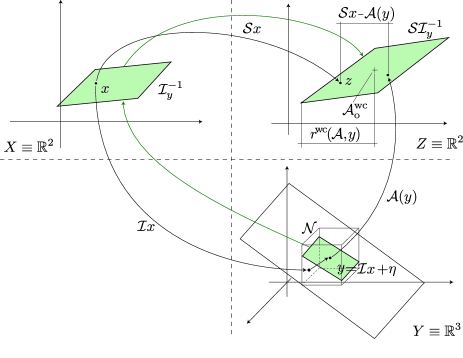
Figure 1: Illustration of the information-based complexity framework.

Let $X$ be a linear normed $n$-dimensional space over the real field, which represents the set of (unknown) problem elements $x\in X$. Define a linear operator ${\cal I}$, called information operator, which maps $X$ into a linear normed $m$-dimensional space $Y$

$${\cal I}:X\rightarrow Y.$$

In general, exact information about the problem element $x\in X$ is not available and only perturbed information, or data, $y\in Y$ is given. That is, we have

$$y={\cal I}x+{\eta}$$ (1)

where ${\eta}$ represents additive noise (or uncertainty) which may be deterministic or random. We assume that ${\eta}\in\mathcal{N}$, where $\mathcal{N}\subseteq{{\mathbb{R}}^{m}}$ is a possibly unbounded set. Due to the presence of uncertainty ${\eta}$, the problem element $x\in X$ may not be easily recovered knowing data $y\in Y$. Then, we introduce a linear operator ${\cal S}$, called a solution operator, which maps $X$ into $Z$

$${\cal S}:X\rightarrow Z$$

where $Z$ is a linear normed $s$-dimensional space over the real field, where $s\leq n$. Given ${\cal S}$, our aim is to estimate an element ${\cal S}x\in Z$ knowing the corrupted information $y\in Y$ about the problem element $x\in X$.

An algorithm ${\cal A}$ is a mapping (in general nonlinear) from $Y$ into $Z$, i.e.

$${\cal A}:Y\rightarrow Z.$$

An algorithm provides an approximation ${\cal A}(y)$ of ${\cal S}x$ using the available information $y\in Y$ of $x\in X$. The outcome of such an algorithm is called an estimate $z={\cal A}(y)$.

We now introduce a set which plays a key role in the subsequent definitions of radius of information and optimal algorithm. Given data $y\in Y$, we define the consistency set as follows

$${{\cal I}^{-1}_{y}}\doteq\left\{x\in X\,:\,y={\cal I}x+{\eta}\text{ for some }{\eta}\in\mathcal{N}\right\}$$ (2)

which represents the set of all problem elements $x\in X$ compatible with (i.e. not invalidated by) ${\cal I}x$, uncertainty ${\eta}$ and bounding set $\mathcal{N}$. For the sake of simplicity, we assume that the three sets $X,Y,Z$ are equipped with the same $\ell_{p}$ norm. Also, in the sequel we assume that the information operator ${\cal I}$ is a one-to-one mapping, i.e. $m\geq n$ and ${\rm rank}\ {\cal I}=n$. Similarly, $n\geq s$ and ${\cal S}$ is full row rank. Moreover, we assume that the set ${{\cal I}^{-1}_{y}}$ has non-empty interior. Note that, in a system identification context, the assumption on ${\cal I}$ and on the consistency set ${{\cal I}^{-1}_{y}}$ are necessary conditions for identifiability of the problem element $x\in X$. Similarly, the assumption of full-rank ${\cal S}$ is equivalent to assuming that the elements of the vector $z={\cal S}x$ are linearly independent (otherwise, one could always estimate a linearly independent set and use it to reconstruct the rest of the vector $z$). We now provide an illustrative example showing the role of these operators and spaces in the context of system identification; note that the IBC theoretical setting also applies to filtering problems, see for instance [50, 22].

Example 1 (System parameter identification and prediction)

Consider a parameter identification problem which has the objective to identify a linear system from noisy measurements. In this case, the problem elements are represented by the trajectory $\xi=\xi(t,x)$ of a dynamic system, parameterized by some unknown parameter vector $x\in X$. This may be represented as the following finite regression

$$\xi(t,x)=\sum_{i=1}^{n}x_{i}\psi_{i}(t)=\Psi^{\top}\!(t)x,$$

with given basis functions $\psi_{i}(t)$, and $\Psi^{\top}\!(t)\doteq\left[\psi_{1}(t)\quad\cdots\quad\psi_{n}(t)\right]$. We suppose that $m$ noisy measurements of $\xi(t,x)$ are available for $t_{1}<t_{2}<\cdots<t_{m}$, that is

$$y={\cal I}x+{\eta}=\left[\Psi(t_{1})\quad\cdots\quad\Psi(t_{m})\right]^{\top}\!x+{\eta}.$$ (3)

In this context, one usually assumes unknown but bounded errors, such that $|{\eta}_{i}|\leq\rho$, $i=1,\ldots,m$, that is $\mathcal{N}=\left\{{\eta}\,:\,\|{\eta}\|\leq\rho\right\}$. Then, the aim is to obtain a parameter estimate using the data $y$. Hence, the solution operator is given by the identity,

$${\cal S}x=x$$

and $Z\equiv X$. The consistency set is sometimes referred to as feasible parameters set, and is given as follows

$${{\cal I}^{-1}_{y}}=\left\{x\in X:\|y-\left[\Psi(t_{1})\,\cdots\,\Psi(t_{m})\right]^{\top}\!x\|_{\infty}\leq\rho\right\}.$$ (4)

For the case of time series prediction, we are interested on predicting $s$ future values of the function $\xi(t,x)$ based on $m$ past measurements, and the solution operator takes the form

$$z = {\cal S}x=\left\{\xi(t_{m+1},x),\quad\ldots\quad,\xi(t_{m+s},x)\right\}$$

$$= \left[\Psi(t_{m+1})\quad\cdots\quad\Psi(t_{m+s})\right]^{\top}\!x.$$

Next, we define approximation errors and optimal algorithms when ${\eta}$ is deterministic or random. First, we briefly summarize the deterministic case which has been deeply analyzed in the literature, see e.g. [37]. The definitions concerning the probabilistic case are new in this context, and are introduced in Section III.

II-A Worst-Case Setting

Given data $y\in Y$, we define the worst-case error $r^{\mathrm{wc}}({\cal A},y)$ of the algorithm ${\cal A}$ as

$$r^{\mathrm{wc}}({\cal A},y)\doteq\max_{x\in{{\cal I}^{-1}_{y}}}\|{\cal S}x-{\cal A}(y)\|.$$ (5)

This error is based on the available information $y\in Y$ about the problem element $x\in X$ and it measures the approximation error between $Sx$ and $A(y)$. An algorithm ${\cal A}^{\mathrm{wc}}_{\mathrm{o}}$ is called worst-case optimal if it minimizes $r^{\mathrm{wc}}({\cal A},y)$ for any $y\in Y$. That is, given data $y\in Y$, we have

$$r^{\mathrm{wc}}_{\mathrm{o}}(y)\doteq r^{\mathrm{wc}}({\cal A}^{\mathrm{wc}}_{\mathrm{o}},y)\doteq\inf_{\cal A}r^{\mathrm{wc}}({\cal A},y).$$ (6)

The minimal error $r^{\mathrm{wc}}_{\mathrm{o}}(y)$ is called the worst-case radius of information.

This optimality criterion is meaningful in estimation problems as it ensures the smallest approximation error between the actual (unknown) solution ${\cal S}x$ and its estimate ${\cal A}(y)$ for the worst element $x\in{{\cal I}^{-1}_{y}}$ for any given data $y\in Y$. Obviously, a worst-case optimal estimate is given by $z^{\mathrm{wc}}_{\mathrm{o}}={\cal A}^{\mathrm{wc}}_{\mathrm{o}}(y)$, see Figure 1.

We notice that optimal algorithms map data $y$ into the $\ell_{p}$–Chebychev center of the set ${\cal S}{{\cal I}^{-1}_{y}}$, where the Chebychev center $z_{\mathrm{c}}(H)$ of a set $H\subseteq Z$ is defined as

$$\max_{h\in H}\|h-z_{\mathrm{c}}(H)\|\doteq\inf_{z\in Z}\max_{h\in H}\|h-z\|\doteq r_{\mathrm{c}}(H).$$

Optimal algorithms are often called central algorithms and $z_{\mathrm{c}}({\cal S}{{\cal I}^{-1}_{y}})=z^{\mathrm{wc}}_{\mathrm{o}}$ is the worst-case optimal estimate, frequently referred to as central estimate. We remark that, in general, the Chebychev center of a set $H\subset Z$ may not be unique (e.g. for $\ell_{\infty}$ norms), and not necessarily belongs to $H$, even if $H$ is convex.

III Probabilistic Setting with Random Uncertainty

In this section, we introduce a probabilistic counterpart of the worst-case setting previously defined. That is we define optimal algorithms ${\cal A}^{\mathrm{pr}}_{\mathrm{o}}$ and the probabilistic radius $r^{\mathrm{pr}}({\cal A},y,\epsilon)$ for the so-called probabilistic setting when the uncertainty ${\eta}$ is random and $\epsilon\in(0,\,1)$ is a given parameter called accuracy. Roughly speaking, in this setting the error of an algorithm is measured in a worst-case sense, but we “discard” a set of measure at most $\epsilon$ from the consistency set ${\cal S}{{\cal I}^{-1}_{y}}$. Hence, the probabilistic radius of information may be interpreted as the smallest radius of a ball discarding a set whose measure is at most $\epsilon$. Therefore, we are decreasing the worst-case radius of information at the expense of a probabilistic “risk” $\epsilon$. In a system identification context, reducing the radius of information is clearly a highly desirable property. Using this probabilistic notion, we compute a trade-off function which shows how the radius of information decreases as a function of the parameter $\epsilon$, as described in the tutorial Example 2 and in the numerical example presented in Section VII.

Formally, in the sequel we assume that the uncertainty ${\eta}$ is a real random vector with given probability measure ${\mu}_{\mathcal{N}}$ over the support set $\mathcal{N}\subseteq{{\mathbb{R}}^{m}}$.

Remark 1 (Induced measure over ${{\cal I}^{-1}_{y}}$)

We note that the probability measure over the set $\mathcal{N}$ induces, by means of equation (1), a probability measure $\tilde{\mu}_{{{\cal I}^{-1}_{y}}}$ over the set ${{\cal I}^{-1}_{y}}$. This induced measure is formally defined in [54, Chapter 6] and it is such that points outside the consistency set ${{\cal I}^{-1}_{y}}$ have measure zero, and $\tilde{\mu}_{{{\cal I}^{-1}_{y}}}\left({{\cal I}^{-1}_{y}}\right)=1$. That is, the induced measure is concentrated over ${{\cal I}^{-1}_{y}}$. We remark that Theorem 1 in Section IV studies the induced measure $\tilde{\mu}_{{{\cal I}^{-1}_{y}}}(\cdot)$ over the set ${{\cal I}^{-1}_{y}}$ when ${\eta}$ is uniformly distributed within $\mathcal{N}$, showing that this measure is still uniform. In turn, the induced measure $\tilde{\mu}_{{{\cal I}^{-1}_{y}}}$ is mapped through the linear operator ${\cal S}$ into a measure over ${\cal S}{{\cal I}^{-1}_{y}}$, which we denote as $\tilde{\mu}_{{\cal S}\!{{\cal I}^{-1}_{y}}}$. In Theorem 1 in Section IV we show that the induced measure $\tilde{\mu}_{{\cal S}\!{{\cal I}^{-1}_{y}}}$ is in general log-concave in the case of uniform density over $\mathcal{N}$. $\diamond$

Given corrupted information $y\in Y$ and accuracy $\epsilon\in(0,1)$, we define the probabilistic error (to level $\epsilon$) $r^{\mathrm{pr}}({\cal A},y,\epsilon)$ of the algorithm ${\cal A}$ as

$$r^{\mathrm{pr}}({\cal A},y,\epsilon)\doteq\inf_{\mathcal{X}_{\epsilon}\text{ such that }\tilde{\mu}_{{{\cal I}^{-1}_{y}}}(\mathcal{X}_{\epsilon})\leq\epsilon}\,\max_{x\,\in\,{{\cal I}^{-1}_{y}}\setminus\mathcal{X}_{\epsilon}}\|{\cal S}x-{\cal A}(y)\|$$ (7)

where the notation ${{\cal I}^{-1}_{y}}\setminus\mathcal{X}_{\epsilon}$ indicates the set-theoretic difference between ${{\cal I}^{-1}_{y}}$ and $\mathcal{X}_{\epsilon}$. Clearly, $r^{\mathrm{pr}}({\cal A},y,\epsilon)\leq r^{\mathrm{wc}}({\cal A},y)$ for any algorithm ${\cal A}$, data $y\in Y$ and accuracy level $\epsilon\in(0,1)$, which implies a reduction of the approximation error in a probabilistic setting.

An algorithm ${\cal A}^{\mathrm{pr}}_{\mathrm{o}}$ is called probabilistic optimal (to level $\epsilon$) if it minimizes the error $r^{\mathrm{pr}}({\cal A},y,\epsilon)$ for any $y\in Y$ and $\epsilon\in(0,1)$. That is, given data $y\in Y$ and accuracy level $\epsilon\in(0,1)$, we have

$$r^{\mathrm{pr}}_{\mathrm{o}}(y,\epsilon)\doteq r^{\mathrm{pr}}({\cal A}^{\mathrm{pr}}_{\mathrm{o}},y,\epsilon)=\inf_{\cal A}r^{\mathrm{pr}}({\cal A},y,\epsilon).$$ (8)

The minimal error $r^{\mathrm{pr}}_{\mathrm{o}}(y,\epsilon)$ is called the probabilistic radius of information (to level $\epsilon$) and the corresponding optimal estimate is given by

$${z}^{\mathrm{pr}}_{\mathrm{o}}(\epsilon)\doteq{\cal A}^{\mathrm{pr}}_{\mathrm{o}}(y,\epsilon).$$ (9)

The problem we study in the next section is the computation of $r^{\mathrm{pr}}_{\mathrm{o}}(y,\epsilon)$ and the derivation of probabilistic optimal algorithms ${\cal A}^{\mathrm{pr}}_{\mathrm{o}}$. To this end, as in [54], we reformulate equation (7) in terms of a chance-constrained optimization problem [39]

$$r^{\mathrm{pr}}({\cal A},y,\epsilon)=\min\left\{r\,:\,v(r,{\cal A})\leq\epsilon\right\},$$

where the violation function for given algorithm ${\cal A}$ and radius $r$ is defined as

$$v(r,{\cal A})\doteq\tilde{\mu}_{{{\cal I}^{-1}_{y}}}\left\{x\in{{\cal I}^{-1}_{y}}\,:\,\|{\cal S}x-{\cal A}(y)\|>r\right\}.$$

Then, this formulation leads immediately to

$$r_{\mathrm{o}}^{\mathrm{pr}}(y,\epsilon)=\min\left\{r\,:\,v_{\mathrm{o}}(r)\leq\epsilon\right\},$$ (10)

where the optimal violation function for a given radius $r$ is given by

$$v_{\mathrm{o}}(r)\doteq\inf_{{\cal A}}\tilde{\mu}_{{{\cal I}^{-1}_{y}}}\left\{x\in{{\cal I}^{-1}_{y}}:\|{\cal S}x-{\cal A}(y)\|>r\right\}.$$ (11)

Roughly speaking, the function $v_{o}(r)$ describes how the risk $\epsilon$ decreases as a function of the radius $r$. However, the computation of $v_{o}(r)$ is not an easy task and requires the results proved in Section IV and the algorithms presented in Section V. To illustrate the notions introduced so far, we consider the following numerical example. The example is tutorial, and it is sufficiently simple so that all relevant sets are two dimensional and can be easily depicted.

Example 2 (Identification of a second order model)

Our aim is to estimate the parameters of a second order FIR model

$$y_{k}=x_{1}u_{k}+x_{2}u_{k-1}+{\eta}_{k},\quad k=1,\ldots,m\\$$ (12)

where the input $u_{k}$ is a known input sequence. The (unknown) nominal parameters were set to $[1.25\quad 2.35]^{\top}\!$, and $m=100$ measurements were collected generating the input sequence $\{u_{k}\}$ according to a Gaussian distribution with zero mean value and unit variance, and the measurement uncertainty ${\eta}$ as a sequence of uniformly distributed noise with $|{\eta}_{k}|\leq 0.5$. Note that, in this case, the operator ${\cal S}$ is the identity, and thus $X\equiv Z$ and the sets ${{\cal I}^{-1}_{y}}$ and ${\cal S}{{\cal I}^{-1}_{y}}$ coincide. That is, the goal is to estimate $z_{i}=x_{i}$, $i=1,2$.

First, the optimal worst-case radius defined in (6) and the corresponding optimal solution have been computed by solving four linear programs (corresponding to finding the tightest box containing the polytope ${\cal S}{{\cal I}^{-1}_{y}}$). The computed worst-case optimal estimate is $z_{\mathrm{o}}^{\mathrm{wc}}=[1.2499\quad 2.3551]^{\top}\!$ and the worst-case radius is $r_{\mathrm{o}}^{\mathrm{wc}}(y)=0.0352$.

Subsequently, we fix the accuracy level $\epsilon=0.1$, and aim at computing a probabilistic optimal radius and the corresponding optimal estimate according to definitions (8) and (9). By using the techniques discussed in Section IV, we obtained $r_{\mathrm{o}}^{\mathrm{pr}}(y,0.1)=0.0284$ and $z_{\mathrm{o}}^{\mathrm{pr}}(0.1)=[1.2480\quad 2.3540]^{\top}\!$, which represents a $25\%$ improvement.

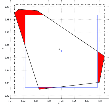
Figure 2: Consistency set and relevant quantities for Example 2. The worst-case optimal radius $r_{\mathrm{o}}^{\mathrm{wc}}(y)$ corresponds to the radius of the dash-dotted box enclosing the polytope ${\cal S}{{\cal I}^{-1}_{y}}$. Its center, denoted by a cross $+$, represents the optimal worst-case estimate $z_{\mathrm{o}}^{\mathrm{wc}}$. The probabilistic optimal (to level $\epsilon=0.1$) radius $r_{\mathrm{o}}^{\mathrm{pr}}(y,\epsilon)$ corresponds to the radius of the solid-line box, which is the “optimal set” ${\cal X}_{\epsilon}$ that, according to definition (7), discards a set of measure $\epsilon$ from ${{\cal I}^{-1}_{y}}$. The discarded set ${{\cal I}^{-1}_{y}}\setminus\mathcal{X}_{\epsilon}$ is represented by the dark (red) area. The center of this box, denoted by a star $\star$, represents the optimal probabilistic estimate $z_{\mathrm{o}}^{\mathrm{pr}}(\epsilon)$.

IV Random Uncertainty Uniformly Distributed

In this section, which contains the main technical results of the paper, we study the case when ${\eta}$ is uniformly distributed over a norm bounded set, and we prove how in this case the computation of the optimal violation function, and thus of the probabilistic optimal estimate, can be formulated as a concave maximization problem. Formally, for a set $A$, the uniform density over $A$ is defined as

$${{\cal U}_{A}}(x)\doteq\left\{\begin{array}[]{cl}\displaystyle 1/\mathrm{vol}\left[A\right]&\mbox{ if }x\in A;\\ 0&\mbox{ otherwise}\end{array}\right.$$

where $\mathrm{vol}\left[A\right]$ represents the Lebesgue measure (volume) of the set $A$, see [24] for details on Lebesgue measures and integration. Note that the uniform density ${{\cal U}_{A}}$ generates a uniform Lebesgue measure $\lambda_{A}$ on $A$, such that, for any Borel measurable set $B$, $\lambda_{A}(B)=\mathrm{vol}\left[B\cap A\right]/\mathrm{vol}\left[A\right]$.

Assumption 1 (Uniform noise over ${\cal B}(r)$)

We assume that ${\eta}$ is uniformly distributed over the $\ell_{p}$ norm-ball ${\cal B}(r)=\left\{{\eta}\,:\,\|{\eta}\|_{p}\leq r\right\}$; that is, $\mathcal{N}={\cal B}(r)$ and $\mu_{\mathcal{N}}=\lambda_{\mathcal{N}}$.

First, we address a preliminary technical question: If ${\mu}_{\mathcal{N}}$ is the uniform measure over $\mathcal{N}$, what is the induced measure $\tilde{\mu}_{{{\cal I}^{-1}_{y}}}$ over the set ${{\cal I}^{-1}_{y}}$ defined in equation (2)? The next result shows that this distribution is indeed still uniform under the mild assumption of compactness of $\mathcal{N}$.

Theorem 1 (Measures over ${{\cal I}^{-1}_{y}}$ and ${\cal S}{{\cal I}^{-1}_{y}}$)

Let $\mathcal{N}$ be a compact set, and let ${\eta}\sim{\cal U}_{\mathcal{N}}$, then, for any $y\in Y$ it holds:

1. The induced measure $\tilde{\mu}_{{{\cal I}^{-1}_{y}}}$ is uniform over ${{\cal I}^{-1}_{y}}$, that is $\displaystyle\tilde{\mu}_{{{\cal I}^{-1}_{y}}}\equiv\lambda_{{{\cal I}^{-1}_{y}}}$;

2. The induced measure $\tilde{\mu}_{{\cal S}\!{{\cal I}^{-1}_{y}}}$ over ${\cal S}{{\cal I}^{-1}_{y}}$ is log-concave. Moreover, if ${\cal S}\in{{\mathbb{R}}^{n,n}}$, then this measure is uniform, that is $\displaystyle\tilde{\mu}_{{\cal S}\!{{\cal I}^{-1}_{y}}}\equiv\lambda_{{\cal S}{{\cal I}^{-1}_{y}}}.$

The proof of this theorem is reported in Appendix A.

Remark 2 (Log-concave measures and Brunn-Minkowski inequality)

Statement (ii) of the theorem proves that the induced measure on ${\cal S}{{\cal I}^{-1}_{y}}$ is log-concave. We recall that a measure $\mu(\cdot)$ is log-concave if, for any compact sets $A$, $B$ and $\alpha\in[0,\,1]$, it holds

$$\mu(\alpha A+(1-\alpha)B)\geq\mu(A)^{\alpha}\mu(B)^{1-\alpha}$$

where $\alpha A+(1-\alpha)B$ denotes the Minkowski sum of the two sets $\alpha A$ and $(1-\alpha)B$. Note that the Brunn-Minkowski inequality [44] asserts that the uniform measure over convex sets is log-concave. Furthermore, any Gaussian measure is log-concave. $\diamond$

We now introduce an assumption regarding the solution operator ${\cal S}$.

Assumption 2 (Regularized solution operator)

In the sequel, we assume that the solution operator is regularized, so that ${\cal S}=\left[\bar{{\cal S}}\;0_{s,n-s}\right]$, with $\bar{{\cal S}}\in{{\mathbb{R}}^{s,s}}$.

Remark 3 (On Assumption 2)

Note that the assumption is made without loss of generality. Indeed, for any full row rank ${\cal S}\in{{\mathbb{R}}^{s,n}}$, we introduce the change of variables $T=\left[T_{1}\;T_{2}\right]$, where $T_{1}$ is an orthonormal basis of the column space of ${\cal S}^{\top}\!$ and $T_{2}$ is an orthonormal basis of the null space of ${\cal S}$. Then, $T$ is orthogonal by definition, and it follows

$$z = {\cal S}x={\cal S}TT^{\top}\!x={\cal S}\left[T_{1}\;T_{2}\right]T^{\top}\!x$$

$$= \left[{\cal S}T_{1}\;{\cal S}T_{2}\right]T^{\top}\!x=\left[\bar{{\cal S}}\;0_{s,n-s}\right]\tilde{x}=\widetilde{{\cal S}}\tilde{x},$$

where we introduced the new problem element $\tilde{x}\doteq T^{\top}\!x$ and the new solution operator $\widetilde{{\cal S}}\doteq{\cal S}T$. Note that, with this change of variables, equation (1) is rewritten as $y=\widetilde{\cal I}\tilde{x}+{\eta},$ by introducing the transformed information operator $\widetilde{\cal I}\doteq{\cal I}T$. We observe that any algorithm ${\cal A}$, being a mapping from $Y$ to $Z$, is invariant to this change of variable. It is immediate to conclude that the new problem defined in the variable $\tilde{x}$ and the operators $\widetilde{\cal I}$ and $\widetilde{\cal S}$ satisfies Assumption 2. $\diamond$

Instrumental to the next developments, we introduce the cylinder in the element space $X$, with given “center” $z_{\mathrm{c}}\in Z$ and radius $r$, as follows

$${\cal C}(z_{\mathrm{c}},r) \doteq \left\{x\in{{\mathbb{R}}^{n}}\,:\,\|{\cal S}x-z_{\mathrm{c}}\|\leq r\right\}$$

$$= {\cal S}^{-1}({\cal B}(z_{\mathrm{c}},r))\subset X,$$

that is, ${\cal C}(z_{\mathrm{c}},r)$ is the inverse image (pre-image) under the solution operator ${\cal S}$ of the $\ell_{p}$ norm-ball ${\cal B}(z_{c},r)\doteq\left\{z\,:\,\|z-z_{c}\|_{p}\leq r\right\}$. Moreover, due to Assumption 2, the cylinder ${\cal C}(z_{\mathrm{c}},r)$ is parallel to the coordinate axes, that is any element $x$ of the cylinder can be written as

$$x\in{\cal C}(z_{\mathrm{c}},r)\Leftrightarrow$$

$$x= \left[\begin{array}[]{c}\bar{{\cal S}}^{-1}\zeta\\ \xi\end{array}\right],\zeta\in{\cal B}(z_{\mathrm{c}},r)\subset{{\mathbb{R}}^{s}},\,\xi\in{{\mathbb{R}}^{n-s}}.$$

Hence, for the case $s<n$, the cylinder is unbounded, while for $s=n$ it is simply a linear transformation through ${\cal S}^{-1}$ of an $\ell_{p}$ norm-ball. Next, for given center $z_{\mathrm{c}}\in Z$ and radius $r>0$, we define the intersection set between the cylinder ${\cal C}(z_{\mathrm{c}},r)$ and the consistency set ${{\cal I}^{-1}_{y}}$

$$\Phi(z_{\mathrm{c}},r)\doteq{{\cal I}^{-1}_{y}}\,\cap\,{\cal C}(z_{\mathrm{c}},r)\subset X$$ (15)

and its volume

$$\phi(z_{\mathrm{c}},r)\doteq\mathrm{vol}\left[\Phi(z_{\mathrm{c}},r)\right].$$ (16)

Finally, we define the set ${\cal H}(r)$ of all centers $z_{\mathrm{c}}\in{{\mathbb{R}}^{s}}$ for which the intersection set $\Phi(z_{\mathrm{c}},r)$ is non-empty, i.e.

$${\cal H}(r)\doteq\left\{z_{\mathrm{c}}\in{{\mathbb{R}}^{s}}\,:\,\Phi(z_{\mathrm{c}},r)\not=\emptyset\right\}.$$ (17)

Note that, even if the cylinder ${\cal C}(z_{\mathrm{c}},r)$ is in general unbounded, the set $\Phi(z_{\mathrm{c}},r)$ is bounded whenever $z_{\mathrm{c}}\in{\cal H}(r)$, since ${{\cal I}^{-1}_{y}}$ is bounded for uniform distributions.

We are now ready to state the main theorem of this section, that provides useful properties from the computational point of view of the optimal violation function defined in (11).

Theorem 2

Under Assumptions 1 and 2, the following statements hold

1. For given $r>0$, the optimal violation function $v_{\mathrm{o}}(r)$ is given by

   $$v_{\mathrm{o}}(r)=1-\frac{\phi_{\mathrm{o}}(r)}{\mathrm{vol}\left[{{\cal I}^{-1}_{y}}\right]},$$ (18)

   where $\phi_{\mathrm{o}}(r)$ is the solution of the optimization problem

   $$\phi_{\mathrm{o}}(r)\doteq\max_{z_{\mathrm{c}}\in{\cal H}(r)}\phi(z_{\mathrm{c}},r)$$ (19)

   with $\phi(z_{\mathrm{c}},r)$ and ${\cal H}(r)$ defined in (16) and (17), respectively;

2. For given $r>0$, the function $\phi(z_{\mathrm{c}},r)$ is quasi-concave for $z_{\mathrm{c}}\in{\cal H}(r)$, and the set ${\cal H}(r)$ is convex;

3. The function $v_{\mathrm{o}}(r)$ is right-continuous and non-increasing for $r>0$.

The proof of this result is reported in Appendix B.

Remark 4 (Unimodality of the function $\phi(z_{\mathrm{c}},r)$)

Point (ii) in Theorem 2 is crucial from the computational viewpoint. Indeed, as remarked for instance in [6], a quasi-concave function cannot have local maxima. Roughly speaking, this means that the function $\phi(\cdot,r)$ is unimodal, and therefore any local maximal solution of problem (19) is also a global maximum. Note that from the Brunn-Minkowski inequality it follows that, if there are multiple points $z_{\mathrm{o}}^{(i)}$ where $\phi(\cdot)$ achieves its global maximum, then the sets $\Phi(z_{\mathrm{o}}^{(i)},r)$ are all homothetic, see [44].

 

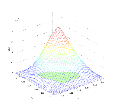
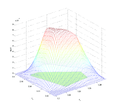
Figure 3: The function $\phi(z_{\mathrm{c}},r)$ for the tutorial problem considered in Example 2, for $r=0.0284$ (a) and $r=0.0150$ (b).

These facts are illustrated in Figure 3, where we plot the function $\phi(z_{\mathrm{c}},r)$ for the tutorial problem considered in Example 2, for two different values of $r$. In the figure on the left, the two sets ${{\cal I}^{-1}_{y}}$ and ${\cal C}(z_{\mathrm{c}},r)$ intersect for all considered values of $z_{\mathrm{c}}$, the function is unimodal, and clearly presents a unique global maximum. In the figure on the right, the radius $r$ is smaller, and there are values of $z_{\mathrm{c}}$ for which ${\cal C}(z_{\mathrm{c}},r)$ is completely contained in ${{\cal I}^{-1}_{y}}$, thus leading to the “flat” region on the top. However, note that this is the only flat region, so that the function is “well-behaved” from an optimization viewpoint. $\diamond$

Remark 5 (Probabilistic radius and probabilistic optimal estimate)

Theorem 2 provides a way of computing the optimal probabilistic radius of information $r_{\mathrm{o}}^{\mathrm{pr}}(y,\epsilon)$. Indeed, the probabilistic radius of information (to level $\epsilon$) is given by the solution of the following one-dimensional inverse problem

$$r^{\mathrm{pr}}_{\mathrm{o}}(y,\epsilon)=\min\left\{r\,:\,v_{\mathrm{o}}(r)\leq\epsilon\right\}.$$ (20)

Note that point (iii) in Theorem 2 guarantees that such solution always exists for $\epsilon\in(0,\,1)$, and it is unique. The corresponding optimal estimate is then given by

$$z_{\mathrm{o}}^{\mathrm{pr}}(\epsilon)={\cal A}^{\mathrm{pr}}_{\mathrm{o}}(y,\epsilon)=z_{\mathrm{o}}(r^{\mathrm{pr}}_{\mathrm{o}}(y,\epsilon)),$$

where we denoted by $z_{\mathrm{o}}(r)$ a solution of the optimization problem (19).

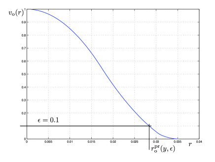
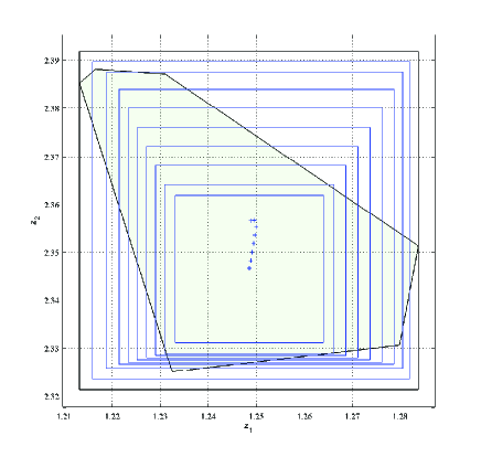
Figure 4: (a) Plot of the function $v_{\mathrm{o}}(r)$ for Example 2, and computation of the optimal probabilistic radius for $\epsilon=0.1$. (b) Plot of the “optimal” $\ell_{\infty}$ balls for different values of $r$. The crosses denote the corresponding optimal estimates $r_{\mathrm{o}}^{\mathrm{pr}}(y,\epsilon)$.

To illustrate, continuing Example 2, we plot in Figure 4(a) the function $v_{\mathrm{o}}(r)$ for $r\in(0,\,r_{\mathrm{o}}^{\mathrm{wc}}]$. We see that $v_{\mathrm{o}}(r)$ is indeed non-increasing (actually, it is strictly decreasing), and hence the inverse problem (20) has clearly a unique solution for any $\epsilon\in(0,\,1)$. $\diamond$

Theorem 2 shows that the problem we are considering is indeed a well-posed one, since it has a unique solution (even though not a unique minimizer in general). However, its solution requires the computation of the volume of the intersection set $\Phi(z_{\mathrm{c}},r)$, which is in general a very hard task. A notable exception in which the probabilistic optimal estimate is immediately computed for ${\eta}$ uniformly distributed in $\mathcal{N}$ is the special case when the consistency set ${{\cal I}^{-1}_{y}}$ is centrally symmetric with center $\bar{x}$. Indeed, in this case it can be seen that ${\cal S}{{\cal I}^{-1}_{y}}$ is also centrally symmetric around $\bar{z}={\cal S}\bar{x}$, and so is the density $\tilde{\mu}_{{\cal S}\!{{\cal I}^{-1}_{y}}}$. Hence, the optimal probabilistic estimate coincides with the center $\bar{z}$, since it follows from symmetry that the probability measure of the intersection of ${\cal S}{{\cal I}^{-1}_{y}}$ with an $\ell_{p}$ norm-ball is maximized when the two sets are concentric. Moreover, this estimate coincides with the classical worst-case (central) estimate, which in turn coincides with the classical least squares estimates.

Remark 6 (Weighted $\ell_{2}$ norms)

Note that the requirement of ${{\cal I}^{-1}_{y}}$ being centrally symmetric is quite demanding in general, but holds naturally when (weighted) $\ell_{2}$ norms are considered, that is when ${\eta}$ is uniformly distributed in a the ball

$$\mathcal{N}=\left\{{\eta}:\|{\eta}\|_{W}\leq\rho\right\},\,\|\xi\|_{W}\doteq\sqrt{\xi^{\top}\!W\xi},W=W^{\top}\!\succ 0,$$

with $W\succ 0$ meaning positive definite, and $\mu_{\eta}(\mathcal{N})=\lambda_{\mathcal{N}}$. This framework has been also considered in the classical set-membership literature, see for instance [29], and it is well-known that in this case the set ${{\cal I}^{-1}_{y}}$ is the ellipsoid

$${{\cal I}^{-1}_{y}} = \left\{x\in X:\|{\cal I}x-y\|_{W}\leq\rho\right\}$$

$$= \left\{x\in X:(x-x^{\mathrm{ls}})^{\top}\!({\cal I}^{\top}\!W{\cal I})(x-x^{\mathrm{ls}})\leq\rho^{2}\right\},$$

centered around the (weighted) least-squares optimal parameter estimate

$$x^{\mathrm{ls}}\doteq\left({\cal I}^{\top}\!W{\cal I}\right)^{-1}{\cal I}^{\top}\!Wy.$$

Hence, it follows from symmetry that, for any $\epsilon\in(0,1)$, the probabilistic optimal estimate to level $\epsilon$ is given by

$$z_{\mathrm{o}}^{\mathrm{pr}}(\epsilon)={\cal A}^{\mathrm{ls}}(y)={\cal S}x^{\mathrm{ls}}(y).$$

However, we are not aware of any closed-form equation for the corresponding probabilistic optimal radius $r_{\mathrm{o}}^{\mathrm{pr}}(y,\epsilon)$, see Section VI for further comments. $\diamond$

Remark 7 (Connections with worst-case and MLE estimates)

Since the paper considers a setup which is somehow in-between classical statistical estimation and set-membership estimation, it is of interest to discuss the differences and analogies between the various approaches. The advantages with respect to the worst-case based set-membership approach, in terms of conservatism reduction, should be evident from the discussion so far, and will be further analyzed in the numerical example of Section VII.

To better clarify the connections with classical stochastic maximum-likelihood estimation (MLE), note that in [52] it is shown that, for the case of uniform noise, the MLE estimates are not unique, and any element of ${\cal S}{{\cal I}^{-1}_{y}}$ is an MLE estimate. Hence, any approach returning estimates belonging to the consistency set is optimal in this sense. In the IBC literature, estimates with the property of belonging to the consistency set are called interpolatory, see eg. [54] for a formal definition. Interpolatory estimates enjoy interesting properties: for instance, it is easy to show that they are almost worst-case optimal (within a factor of 2). In particular, it can be shown, using results from convex analysis [2], that in the case of uniform noise bounded in the $\ell_{2}$ norm, both the central estimate obtained in the set-membership approach and the probabilistic optimal estimate are indeed interpolatory. Hence, in this case, our approach can be seen as a tool for selecting an optimal MLE solution.

The situation is more complicated for $\ell_{1}$ or $\ell_{\infty}$ norms, because in this case the central estimate is not always interpolatory. Similarly, the probabilistic optimal estimate defined in (8) is not necessarily interpolatory. Furthermore, we note that in this case also the classical least-squares estimate may lie outside the consistency set ${\cal S}{{\cal I}^{-1}_{y}}$, hence it is not MLE. For instance, in Example 2 the least-squares estimate can be immediately computed as $x^{\mathrm{ls}}=[1.2873\quad 2.3190]^{\top}\!$ and it is indeed not interpolatory.

An interesting approach, in the case of $\ell_{1}$ or $\ell_{\infty}$ norms, could be indeed to consider a conditional probabilistic-optimal estimate,which requires looking for the best interpolatory estimate minimizing the probabilistic radius (7). Note that, from a computational viewpoint, this is immediately obtained constraining the optimization problem (19) to $z_{\mathrm{c}}\in{\cal S}{{\cal I}^{-1}_{y}}$.

V Randomized and deterministic algorithms for optimal violation function approximation

In this section, we concentrate on the solution of the optimization problem defined in (19), Theorem 2 for fixed $r>0$. For simplicity, we restate this problem dropping the subscript from $z_{\mathrm{c}}$

(P-max-int) : $$\max_{z\in{\cal H}(r)}\phi(z,r),$$

$$\quad\phi(z,r)=\mathrm{vol}\left[{{\cal I}^{-1}_{y}}\,\cap\,{\cal C}(z,r)\right].$$

First, note that this problem is computationally very hard in general. For instance, for $\ell_{1}$ or $\ell_{\infty}$ norms, the consistency set ${{\cal I}^{-1}_{y}}$ is a polytope and ${\cal C}(z,r)$ is a cylinder parallel to the coordinate axes whose cross-section is a polytope. Hence, even evaluating the function $\phi(z,r)$ appearing in (V) amounts to computing the volume of a polytope, and this problem has been shown to be NP-hard in [32].

Remark 8 (Volume oracle and oracle-polynomial-time algorithm)

For the case of polytopic sets, the papers [1, 21] study the problem (P-max-int) in the hypothetical setting that an oracle exists which satisfies the following property: given $r>0$ and $z\in{\cal H}(r)$, it returns the value of the function $\phi(z,r)$, together with a sub-gradient of it. In this case, in [1] a strongly polynomial-time (in the number of oracle calls) algorithm is derived. Note that, even if the problem is NP hard in general, one can compute the volume of a polytope in a reasonable time for considerably complex polytopes in modest (e.g. for $n\leq 10$) dimensions, see [7]. In this particular case, for $\ell_{\infty}$ norms, the method proposed by [21] may be used. For instance, for Example 2, all relevant quantities have been computed exactly by employing this method. However it should be remarked that, for larger dimensions, the curse of dimensionality makes the problem computationally intractable, and alternative methods need to be devised. $\diamond$

In the next subsections, we develop random and deterministic relaxations of problem (P-max-int) which do not suffer from these computational drawbacks.

V-A Randomized algorithms for computing (P-max-int)

In this section, we propose randomized algorithms based on a probabilistic volume oracle and a stochastic optimization approach for approximately solving problem (P-max-int) for $\ell_{p}$ norms. First of all, we compute a bounded version of the cylinder ${\cal C}(z,r)$. To this end, we note that bounds $x_{i}^{-}$, $x_{i}^{+}$ on the variables $x_{i}$, $i=s+1,\ldots,n$, can be obtained as the solution of the following $2(n-s)$ convex programs,

$$\begin{array}[]{lll}x_{i}^{-}=&\min\,x_{i}&\\ &\text{\rm subject to}&x\in{{\cal I}^{-1}_{y}}\end{array},$$ (25)

$$\begin{array}[]{lll}x_{i}^{+}=&\max\,x_{i}&\\ &\text{\rm subject to}&x\in{{\cal I}^{-1}_{y}}\end{array},$$ (28)

$$i=s+1,\ldots,n.$$ (29)

The problems above are convex, and for $\ell_{p}$ norms can be solved for instance by (sub)gradient-based or interior point methods. In particular, problem (29) reduces to the solution to $2(n-s)$ linear programs for $\ell_{1}$ or $\ell_{\infty}$ norms. Then, under Assumption 2, we define the cylinder

$$\overline{\cal C}(z,r) \doteq \left\{x\in{{\mathbb{R}}^{n}}\,:\,\left\|\bar{{\cal S}}\left[\begin{smallmatrix}x_{1}\\ \vdots\\ x_{s}\end{smallmatrix}\right]-z\right\|\leq r,\right.$$

$$\quad\left.x_{i}^{-}\leq x_{i}\leq x_{i}^{+},i=s+1,\ldots,n\right\}.$$

Note that the cylinder $\overline{\cal C}(z,r)$ is bounded, and has volume equal to

$$\mathrm{vol}\left[\overline{\cal C}(z,r)\right]\!=\!\frac{(2r)^{s}\Gamma^{s}\left(1/p+1\right)}{|\det(\bar{{\cal S}})|\Gamma\left(s/p+1\right)}\!\!\prod_{i=s+1}^{n}(x_{i}^{+}-x_{i}^{-})\doteq\mathrm{V}_{{\cal C}}$$ (31)

where $\Gamma(\cdot)$ denotes the Gamma function. By construction, we have that, for any $r>0$ and $z\in{\cal H}(r)$, $\Phi(z,r)={{\cal I}^{-1}_{y}}\,\cap\,\overline{\cal C}(z,r).$ Note that independent and identically distributed (iid) random samples inside $\overline{\cal C}(z,r)$ can be easily obtained from iid uniform samples in the $\ell_{p}$-norm ball, whose generation is studied in [9]. Then, a probabilistic approximation of the volume of the intersection $\Phi(z,r)$ may be computed by means of the randomized oracle presented in Algorithm 1, which is based on the uniform generation of iid samples in $\overline{\cal C}(z,r)$.

Algorithm 1 Probabilistic Volume Oracle

• Random Generation
  Generate $N$ iid uniform samples $\zeta^{(1)},\ldots,\zeta^{(N)}$ in the $s$-dimensional ball ${\cal B}(z,r)$

  • For $i=1$ to $N$

    • Generate $s$ iid scalars $\gamma_{j}$ according to the unilateral Gamma density

      $$G_{a,b}(x)=\frac{1}{\Gamma(a)b^{a}}x^{a-1}\mathrm{e}^{-x/b},\quad x\geq 0,$$ (32)

      with parameters $a=1/p,b=1$

    • Construct the vector $\eta\in{\mathbb{R}}^{n}$ of components $\eta_{j}=s_{j}\gamma_{j}^{1/p}$, where $s_{j}$ are iid random signs

    • Let $\zeta^{(i)}=z+r\,w^{1/n}\,\frac{\eta}{\|\eta\|_{p}}$ where $w$ is uniform in $[0,1]$

    End for

• Generate $N$ iid uniform samples $\xi^{(1)},\ldots,\xi^{(N)}$

  • For $i=1$ to $N$

    • Generate $\xi_{j}^{(i)}$ uniformly in the interval $[x_{s+j}^{-},\,x_{s+j}^{+}]$, $j=1,\ldots,n-s$

    End for

• Construct the random samples in $\overline{\cal C}(z,r)$ as follows

  $$\chi^{(i)}=\begin{bmatrix}\bar{{\cal S}}^{-1}\zeta^{(i)}\\ \xi^{(i)}\end{bmatrix},\quad i=1,\ldots,N$$

• Consistency Test

  • Compute the number of samples inside ${{\cal I}^{-1}_{y}}$ as follows

    $$N_{g}=\sum_{i=1}^{N}\mathbb{I}\left(\|{\cal I}\,\chi^{(i)}-y\|\leq\rho\right)$$

    where $\mathbb{I}\left(\cdot\right)$ denotes the indicator function, which is equal to one if the argument is true, and it is zero otherwise.

• Probabilistic Oracle Return an approximation of the volume $\phi(z,r)$ as follows

  $$\widehat{\phi}_{N}(z,r)=\frac{N_{g}}{N}\mathrm{V}_{{\cal C}}$$

  where $\mathrm{V}_{{\cal C}}$ is defined in (31).

Note that the expected value of the random variable $\widehat{\phi}_{N}(z,r)$ with respect to the samples $\chi^{(1)},\ldots,\chi^{(N)}\in\overline{\cal C}(z,r)$ is exactly the volume function $\phi(z,r)$ appearing in (P-max-int) that is

$$\mathbb{E}\left[\widehat{\phi}_{N}(z,r)\right]=\phi(z,r).$$

This immediately follows from linearity of the expected value

$$\mathbb{E}\left[\widehat{\phi}_{N}(z,r)\right] = \mathbb{E}\left[\frac{1}{N}\sum_{i=1}^{N}\mathbb{I}\left(\chi^{(i)}\in{{\cal I}^{-1}_{y}}\right)\mathrm{V}_{{\cal C}}\right]$$

$$= \frac{1}{N}\sum_{i=1}^{N}\mathbb{E}\left[\mathbb{I}\left(\chi^{(i)}\in{{\cal I}^{-1}_{y}}\right)\right]\mathrm{V}_{{\cal C}}.$$

Then, we have

$$\mathbb{E}\left[\mathbb{I}\left(\chi^{(i)}\in{{\cal I}^{-1}_{y}}\right)\right] = \mathrm{Prob}\left\{\chi^{(i)}\in{{\cal I}^{-1}_{y}}\right\}$$

$$= \mathrm{vol}\left[\Phi(z,r)\right]/\mathrm{vol}\left[\bar{\cal C}(z,r)\right]$$

$$= \phi(z,r)/\mathrm{V}_{{\cal C}}.$$

Hence, we reformulate the problem (P-max-int) as the following stochastic optimization problem

$$\max_{z\in{\cal H}(r)}\mathbb{E}\left[\widehat{\phi}_{N}(z,r)\right].$$

This problem is classical and different stochastic approximation algorithms have been proposed, see for instance [34, 45] and references therein. In particular, in this paper, we use the SPSA (simultaneous perturbations stochastic approximation) algorithm, first proposed in [47], and further discussed in [49]. Convergence results under different conditions are detailed in the literature, see in particular the paper [26] which applies to non-differentiable functions.

Remark 9 (Scenario-based algorithms)

An alternative approach based on randomized methods can be also devised employing results on the scenario optimization method introduced in [8]. In particular, exploiting the results on discarded constraints, see [12, 14], an alternative algorithm can be constructed. The idea is as follows: (i) generate $N$ samples $\chi^{(i)}$ in ${{\cal I}^{-1}_{y}}$ according to the induced measure $\tilde{\mu}_{{{\cal I}^{-1}_{y}}}$, ii) solve the discarded-constraint random program

$$\min_{z,\gamma} \gamma$$ (33)

s.t. $$\frac{1}{L}\sum_{i\in I_{L}}\mathbb{I}\left(\|{\cal S}\chi^{(i)}-z)\|\geq\gamma\right)\leq\epsilon$$

where $I_{L}$ is a set of $L$ indices constructed discarding in a prescribed way $N-L$ indices from the set $1,2,\ldots,N$. Then, in [12, 14] it is shown how to choose $N$ and the discarded set $I_{L}$ to guarantee, with a prescribed level of confidence, that the result of optimization problem (33) is a good approximation of the true probabilistic radius $r_{\mathrm{o}}^{\mathrm{pr}}(y,\epsilon)$. However, this approach entails many seriuos technical difficulties, such as the random sample generation in point (i) and the optimal discarding procedure in point (ii), whose detailed analysis goes beyond the scope of this paper. $\diamond$

V-B A semi-definite programming relaxation to (P-max-int)

In this section, we propose a deterministic approach to (P-max-int) based on a semidefinite relaxation of the problem for $\ell_{\infty}$ norms (extensions to $\ell_{1}$ and $\ell_{2}$ norms are briefly discussed in Remark 10). First note that, in the case of $\ell_{\infty}$ norms, $\mathcal{N}$ is an hypercube of radius $\rho$ and therefore ${{\cal I}^{-1}_{y}}$ is the polytope ${\cal P}_{X}$ defined by the following linear inequalities

$${{\cal I}^{-1}_{y}} = \left\{x\in{{\mathbb{R}}^{n}}\,:\,\|{\cal I}x-y\|_{\infty}\leq\rho\right\}$$ (34)

$$= \left\{x\in{{\mathbb{R}}^{n}}\,:\,\left[\begin{array}[]{c}{\cal I}\\ -{\cal I}\end{array}\right]x\leq\left[\begin{array}[]{c}\rho\mathbf{1}+y\\ \rho\mathbf{1}-y\end{array}\right]\right\}\doteq{\cal P}_{X}$$ (39)

where $\mathbf{1}$ is a vector of ones, $\mathbf{1}=[1\;1\,\cdots\,1]^{\top}\!$. Since the exact computation of the volume of the intersection of two polytopic sets is in general costly and prohibitive in high dimensions, as discussed in Remark 8, we propose to maximize a suitably chosen lower bound of this volume. This lower bound can be computed as the solution of a convex optimization problem. The idea is to construct, for fixed $r>0$, the maximal volume ellipsoid contained in the intersection $\Phi(z,r)$, which requires to solve the optimization problem

$$\max_{z,x_{{\cal E}},P_{{\cal E}}} \mathrm{vol}\left[{\cal E}(x_{{\cal E}},P_{{\cal E}})\right]$$ (40)

subject to $${\cal E}(x_{{\cal E}},P_{{\cal E}})\subseteq\Phi(z,r),$$

where the ellipsoid of center $x_{{\cal E}}$ and shape matrix $P_{{\cal E}}$ is

$${\cal E}(x_{{\cal E}},P_{{\cal E}})\doteq\left\{x\in{{\mathbb{R}}^{n}}\,:\,x=x_{{\cal E}}+P_{{\cal E}}w,\|w\|_{2}\leq 1\right\}.$$

The problem of deriving the maximum volume ellipsoid inscribed in a polytope is a well-studied one, and concave reformulations based on linear matrix inequalities (LMI) are possible, see for instance [5, 4]. For completeness, we report this result in the next theorem.

Theorem 3

Let Assumptions 1 and 2 hold. Then, for given $r>0$, a center that achieves a global optimum for problem (40) can be computed as the solution of the following semi-definite programming (SDP) problem

$$z_{\mathrm{o}}^{\mathrm{sdp}}(r)\in\arg_{z}\,\min_{z,x_{{\cal E}},P_{{\cal E}}}-\log\det P_{{\cal E}}$$

$$\text{\rm subject to }P_{{\cal E}}\succeq 0\quad\text{\rm and}$$ (47)

$$\left[\begin{array}[]{cc}(\rho+e_{i}^{\top}\!(y-{\cal I}x_{{\cal E}}))I_{n}&P_{{\cal E}}{\cal I}^{\top}\!e_{i}\\ \star&\rho+e_{i}^{\top}\!(y-{\cal I}x_{{\cal E}})\end{array}\right]\succeq 0,$$

$$i=1,\ldots,m$$

$$\left[\begin{array}[]{cc}(\rho-e_{i}^{\top}\!(y-{\cal I}x_{{\cal E}}))I_{n}&-P_{{\cal E}}{\cal I}^{\top}\!e_{i}\\ \star&\rho-e_{i}^{\top}\!(y-{\cal I}x_{{\cal E}})\end{array}\right]\succeq 0,$$

$$i=1,\ldots,m$$ (48)

$$\left[\begin{array}[]{cc}(r+\bar{e}_{i}^{\top}\!(z-{\cal S}x_{{\cal E}}))I_{n}&P_{{\cal E}}{\cal S}^{\top}\!\bar{e}_{i}\\ \star&r+\bar{e}_{i}^{\top}\!(z-{\cal S}x_{{\cal E}})\end{array}\right]\succeq 0,$$ (51)

$$i=1,\ldots,s$$ (52)

$$\left[\begin{array}[]{cc}(r-\bar{e}_{i}^{\top}\!(z-{\cal S}x_{{\cal E}}))I_{n}&P_{{\cal E}}{\cal S}^{\top}\!\bar{e}_{i}\\ \star&r-\bar{e}_{i}^{\top}\!(z-{\cal S}x_{{\cal E}})\end{array}\right]\succeq 0,$$ (55)

$$i=1,\ldots,s,$$ (56)

where $e_{i}$ and $\bar{e}_{i}$ are elements of the canonical basis of ${{\mathbb{R}}^{m}}$ and ${{\mathbb{R}}^{s}}$, respectively. Moreover, for all $r>0$, $v_{\mathrm{o}}^{\mathrm{sdp}}(r)\geq v_{\mathrm{o}}(r)$, where we defined

$$v_{\mathrm{o}}^{\mathrm{sdp}}(r)\doteq 1-\frac{\phi\left(z_{\mathrm{o}}^{\mathrm{sdp}}(r),r\right)}{\mathrm{vol}\left[{{\cal I}^{-1}_{y}}\right]}.$$

Proof:

The theorem is immediately proved seeing that (47), (48) impose that ${\cal E}(x_{{\cal E}},P_{{\cal E}})\subseteq{{\cal I}^{-1}_{y}}$ while (52), (56) impose that ${\cal E}(x_{{\cal E}},P_{{\cal E}})\subseteq{\cal C}(z,r)$. This problem is an SDP since the equations are linear matrix inequalities in the variables $z,x_{{\cal E}},P_{{\cal E}}$, and the cost function is convex in $P_{{\cal E}}$. $\square$

From Theorem 3, if follows that the SDP relaxation leads to a suboptimal violation function $v_{\mathrm{o}}^{\mathrm{sdp}}(r)$.

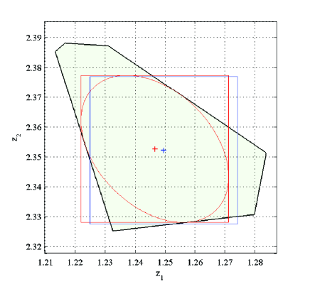
Figure 5: Optimal $\ell_{\infty}$ ball for Example 2, for $r=0.0284$ (in blue), and optimal ball computed as the solution of the SDP relaxation, with corresponding ellipse ${\cal E}(x_{{\cal E}},P_{{\cal E}})$ (in red).

Remark 10 (SDP relaxations for $\ell_{1}$ and $\ell_{2}$)

An approach identical to that proposed in Theorem 3 can be developed for the $\ell_{1}$ norm, considering that also in this case the sets ${{\cal I}^{-1}_{y}}$ and ${\cal C}(z,r)$ are a polytope and a cylinder with polytopic basis, respectively. Similarly, an analogous algorithm can be devised for the (weighted) $\ell_{2}$ norm. In this case, the volume of an ellipsoid contained in the intersection of ${{\cal I}^{-1}_{y}}$ and ${\cal C}(z,r)$ should be maximized, which are respectively the ellipsoid defined in (6) and a cylinder with spherical basis. It can be easily seen, see e.g. [5], that this latter problem can be easily rewritten as a convex SDP optimization problem. $\diamond$

VI Random Uncertainty Normally Distributed and Connections with Least-Squares

In this section, we concentrate on the case when the uncertainty ${\eta}$ is normally distributed with mean value $\bar{v}$ and covariance matrix $\Sigma=\sigma^{2}I\succ 0$, and the set $\mathcal{N}$ coincides with ${{\mathbb{R}}^{m}}$. This permits to draw a bridge between the probabilistic setting introduced in this paper and the classical theory of statistical estimation, which is usually based on additive noise normally distributed. Indeed, it is well known, see e.g. [30, 35] that the minimum variance unbiased estimate for the linear regression model (1) is given by the Gauss-Markov estimate

$$x^{\mathrm{ls}}=\left({\cal I}^{\top}\!\Sigma^{-1}{\cal I}\right)^{-1}{\cal I}^{\top}\!\Sigma^{-1}y,$$

which coincides with the (weighted) least-squares estimate discussed in Remark 6, for $W=\Sigma^{-1}$.

We first remark that this minimum variance problem falls into the average setting of IBC, see [54]. In particular, we recall that this setting has the objective of minimizing the expected value of the estimation error, that is, for given $y$, the optimal average radius is defined as

$$r^{\mathrm{av}}_{\mathrm{o}}(y)\doteq\inf_{\cal A}\left(\mathbb{E}\left[\|{\cal S}x-{\cal A}(y)\|^{2}\right]\right)^{1/2},$$ (57)

where $\mathbb{E}\left[\cdot\right]$ denotes the expected value taken with respect to the conditional measure $\tilde{\mu}_{{{\cal I}^{-1}_{y}}}$ introduced in Remark 1 (which is also Gaussian, due to well-known properties of normal measures). It follows that the optimal average estimate is immediately given by

$$z_{\mathrm{o}}^{\mathrm{av}}={\cal S}x^{\mathrm{ls}},$$

for any $y\in Y$. Moreover, in [54, Chapter 6] it is proven that the optimal average radius does not depend on the measurement $y$, and it can be computed in closed form as

$$r^{\mathrm{av}}_{\mathrm{o}}=r^{\mathrm{av}}_{\mathrm{o}}(y)=\sqrt{\mathrm{Trace}\left({\cal S}\left({\cal I}^{\top}\!\Sigma^{-1}{\cal I}\right)^{-1}{\cal S}^{\top}\!\right)}.$$

For what concerns the probabilistic optimal estimate, we first remark that in the case of normally distributed noise, the definition of the probabilistic radius (7) still applies, observing that the consistency set ${{\cal I}^{-1}_{y}}$ defined in (2) in this case is given by

$${{\cal I}^{-1}_{y}}\doteq\left\{x\in X\,:\,y={\cal I}x+{\eta},\;{\eta}\in{{\mathbb{R}}^{n}}\right\},$$

and is unbounded. Hence, the “discarded” set ${\cal X}_{\epsilon}$ in (7) can be also unbounded. Note that this is not an issue, since $\tilde{\mu}_{{{\cal I}^{-1}_{y}}}$ is defined over all ${{\mathbb{R}}^{n}}$, so that the measure of unbounded sets is well defined.

Similarly to the worst-case and the average settings, the optimality properties of the least-square solution still hold for the probabilistic setting. Indeed, in [54, Chapter 8] it is proven that the optimal probabilistic estimate (to level $\epsilon$) for normal distributions is given by

$$z_{\mathrm{o}}^{\mathrm{pr}}={\cal S}x^{\mathrm{ls}},$$

for any $y\in Y$. Closed-form solutions for the computation of the probabilistic radius $r^{\mathrm{pr}}_{\mathrm{o}}(\epsilon)$ are not available, and in [54, Chapter 8] the following upper bound is given

$$r^{\mathrm{pr}}_{\mathrm{o}}(\epsilon,y)\leq\sqrt{2\ln\frac{5}{\epsilon}}\,r^{\mathrm{av}}_{\mathrm{o}},\quad\text{ for all }y\in Y.$$

However, it is also observed that this bound is essentially sharp when the noise variance is sufficiently small.

VII Numerical example

As a numerical example, we consider a randomly generated instance of (1) with uniform distributed noise. In particular, $m=150$ random measurements of an unknown $n=5$ dimensional vector were drawn taking

$${\cal I} = \mathtt{round(20*rand(m,n)-10)}$$ (58)

$${\eta} = \rho\mathtt{(2*rand(m,1)-1)},$$

with $\rho=5$, and considering as “true” parameters $x^{\mathrm{true}}$ the unit vector. The solution operator was chosen as

$${\cal S}=\left[\begin{array}[]{ccccc}-5&10&-7&0&0\\ 3&-4&7&0&0\\ 2&6&4&0&0\end{array}\right],$$

leading to $z^{\mathrm{true}}={\cal S}x^{\mathrm{true}}=[-2\;6\;12]^{\top}\!$. First, the optimal worst-case radius and the corresponding optimal solution have been computed by solving 10 linear programs (corresponding to finding the tightest box containing the polytope ${\cal S}{{\cal I}^{-1}_{y}}$, see [37]). The computed worst-case optimal estimate is $z_{\mathrm{o}}^{\mathrm{wc}}=[-1.831\;5.839\;11.883]^{\top}\!$ and the worst-case radius is $r_{\mathrm{o}}^{\mathrm{wc}}(y)=0.5791$.

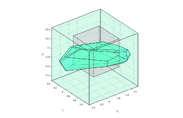
Figure 6: Consistency set, and optimal “box” discarding a set of measure $\epsilon=0.1$. The probabilistic optimal radius $r_{\mathrm{o}}^{\mathrm{pr}}(y,0.1)$ corresponds to the radius of this box. The center, denoted by a star, represents the optimal probabilistic estimate $z_{\mathrm{o}}^{\mathrm{pr}}(y)$.

Subsequently, in order to apply the proposed probabilistic framework, we fixed the accuracy level to $\epsilon=0.1$, and computed the probabilistic optimal radius and the corresponding optimal estimate according to definitions (8) and (9). In this case, we were still able to use the techniques discussed in Remark 8 for computing (P-max-int) exactly. By employing a simple bisection search algorithm over $v_{\mathrm{o}}(r)$, the probabilistic radius of information was computed as $r_{\mathrm{o}}^{\mathrm{pr}}(y,0.1)=0.3074$. The corresponding optimal probabilistic estimate is given by and $z_{\mathrm{o}}^{\mathrm{pr}}(0.1)=[-1.773\;5.869\;11.969]^{\top}\!$. Note that the reduction in terms of radius of information is quite significant, being of the order of $50\%$. The meaning of our approach is well explained in Figure 6. Indeed, in this figure we see that we look for the optimal “box” discarding a set of probability measure $\epsilon=0.1$. Note that, in this figure, the volume of the “discarded set” is clearly more than $10\%$ of the total volume. The reason of this is that the probability of the discarded set is measured in the (five dimensional) space $X$. Figure 7 shows a plot of the violation function $v_{o}(r)$ computed using the different techniques discussed in this paper. It can be observed that all methods provide very consistent results.

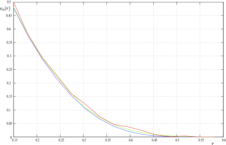
Figure 7: Function $v_{\mathrm{o}}(r)$ for the numerical example. The blue line is the solution obtained computing the volume using the deterministic techniques discussed in Remark 8, the red line corresponds to the SPSA-algorithm and the green one is the SDP relaxation.

Then, to compare, we run $N=10,000$ random experiments, generating each time a difference instance of (ex-instance), and for each we computed the least-square estimate $z^{\mathrm{ls}}={\cal S}x^{\mathrm{ls}}$, the worst-case optimal estimate $z_{\mathrm{o}}^{\mathrm{wc}}$, and the probabilistic optimal estimate $z_{\mathrm{o}}^{\mathrm{pr}}$. Figure 8 shows the (normalized) relative frequency histograms for the three estimates, while Table I reportes the mean and variances of the different estimates and their corresponding errors. It can be seen that both mean and variance of the error of the proposed probabilistic estimate are much smaller than the least-squares one, and also smaller than the worst-case one.

TABLE I: Mean and variance of least-squares, worst-case and probabilistic optimal estimates and corresponding errors

	Mean	Variance
$z^{\mathrm{ls}}$	-2.0035   6.0017   11.9993	0.2618   0.1117   0.0933
$z_{\mathrm{o}}^{\mathrm{wc}}$	-2.0007   6.0005   12.0006	0.0420   0.0183   0.0151
$z_{\mathrm{o}}^{\mathrm{pr}}$	-2.0008   6.0004   12.0004	0.0364   0.0162   0.0140
$\|z_{\mathrm{o}}^{\mathrm{ls}}-z^{\mathrm{true}}\|_{\infty}$	0.4764	0.0762
$\|z_{\mathrm{o}}^{\mathrm{wc}}-z^{\mathrm{true}}\|_{\infty}$	0.1864	0.0148
$\|z_{\mathrm{o}}^{\mathrm{pr}}-z^{\mathrm{true}}\|_{\infty}$	0.1725	0.0134

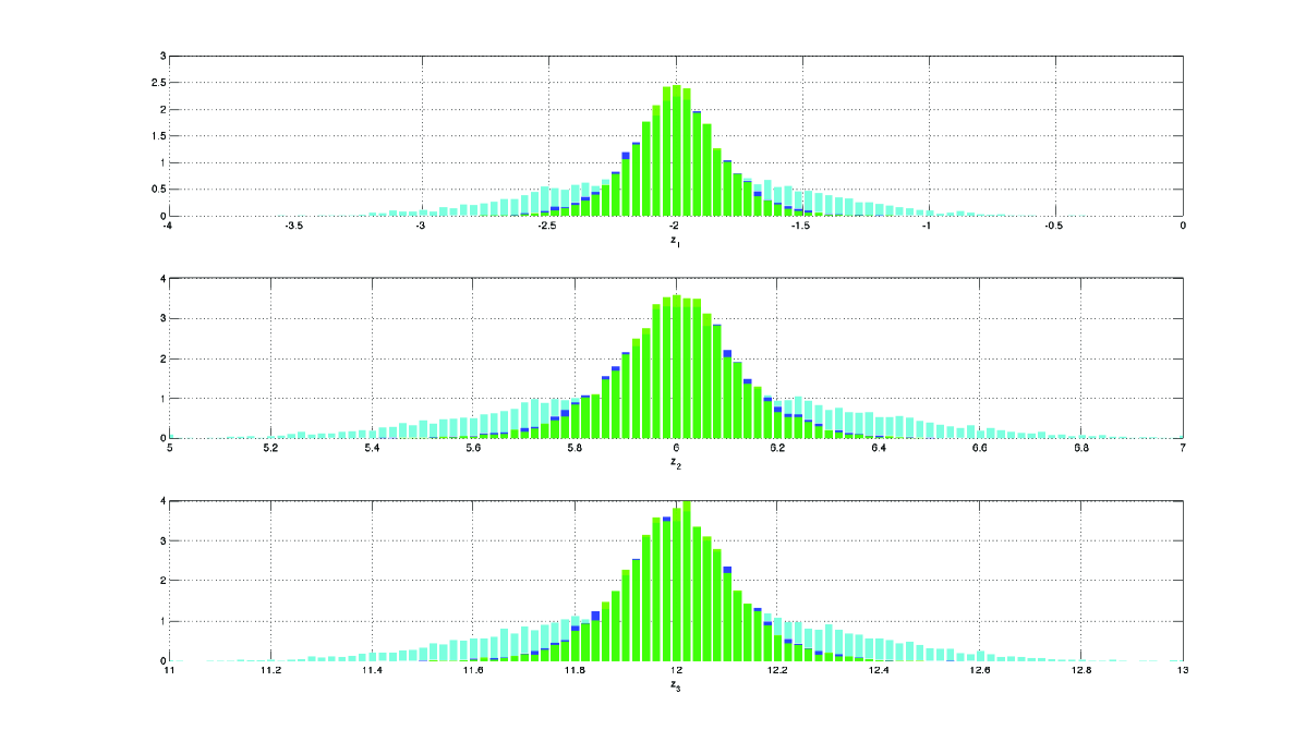
Figure 8: Relative frequencies for least-square estimates (cyan), worst-case optimal estimate (blue) and probabilistic-optimal (green). To allow comparison, the histograms have been normalized so that so that the area under the bars is equal to one.

VIII Conclusions

This paper deals with the rapprochement between the stochastic and worst-case settings for system identification. The problem is formulated within the probabilistic setting of information-based complexity, and it is focused on the idea of discarding sets of small measure from the set of deterministic estimates. The paper establishes rigorous optimality properties of a trade-off curve, called violation function, which shows how the radius of information decreases as a function of the accuracy. Subsequently, randomized and deterministic algorithms for computing the optimal violation function have been presented. Their performance has been successfully tested on a numerical example.

IX Acknowledgements

The authors would like to thank Prof. Takayuki Wada for the enlightening discussions about stochastic optimization, and for clarifying the quasi-concavity properties in Theorem 2, and Prof. Libor Vesely for clarifying properties of the Chebychev center of convex sets. The authors are also indebted to the anonymous reviewers for the numerous comments that allowed to improve the content of the paper.

Appendix A Proof of Theorem 1

Consider the transformation matrix $T=\left[T_{1}\;T_{2}\right]$, where $T_{1}$ is an orthonormal basis of the column space of ${\cal I}$ and $T_{2}$ is an orthonormal basis of the null space of ${\cal I}^{\top}\!$. Furthermore, define the linear transformation $\bar{\eta}\doteq T^{\top}\!{\eta}$, and the set $\bar{\mathcal{N}}\doteq\left\{\bar{\eta}\in{{\mathbb{R}}^{m}}\,:\,T^{-\!\top}\bar{\eta}\in\mathcal{N}\right\}$. Then, if the random variable ${\eta}$ is uniform on $\mathcal{N}$, the linearly transformed random variable $\bar{\eta}$ is uniform on $\bar{\mathcal{N}}$ (see e.g. [24]). Next, by multiplying equation (1) from the left by $T^{\top}\!\!\!$, and defining $\bar{\cal I}_{1}\doteq T_{1}^{\top}\!{\cal I}$ and $\bar{y}_{i}\doteq T_{i}^{\top}\!y$, $\bar{\eta}_{i}\doteq T_{i}^{\top}\!{\eta}$, $i=1,2$, we get

$$\left\{\begin{array}[]{lcll}\bar{\cal I}_{1}x&+&\bar{\eta}_{1}&=\bar{y}_{1}\\ &&\bar{\eta}_{2}&=\bar{y}_{2},\end{array}\right.$$ (59)

since, by construction, $T_{2}^{\top}\!{\cal I}=0$. It follows from definition (2) that a point $x\in X$ belongs to ${{\cal I}^{-1}_{y}}$ if and only if there exists $\bar{\eta}=\left[\begin{smallmatrix}\bar{\eta}_{1}\\ \bar{\eta}_{2}\end{smallmatrix}\right]\in\bar{\mathcal{N}}$ such that (59) holds, i.e. if there exist $\bar{\eta}_{1}$ in the set $\bar{\mathcal{N}}_{1}\doteq\left\{\bar{\eta}_{1}\in{{\mathbb{R}}^{n}}\,:\,\left[\begin{smallmatrix}\bar{\eta}_{1}\\ \bar{y}_{2}\end{smallmatrix}\right]\in\bar{\mathcal{N}}\right\}$ for which $\bar{\cal I}_{1}x+\bar{\eta}_{1}=\bar{y}_{1}$. Note that the set $\bar{\mathcal{N}}_{1}$ represents the intersection of the set $\bar{\mathcal{N}}$ with the hyperplane $\left\{\bar{\eta}=\left[\begin{smallmatrix}\bar{\eta}_{1}\\ \bar{\eta}_{2}\end{smallmatrix}\right]\in{{\mathbb{R}}^{m}}\,:\,\bar{\eta}_{2}=\bar{y}_{2}\right\}$. Since $\bar{\eta}$ is uniform on $\bar{\mathcal{N}}$, it is also uniform on any subset of $\bar{\mathcal{N}}$, and in particular on this intersection set. Hence, $\bar{\eta}_{1}$ is uniformly distributed on $\bar{\mathcal{N}}_{1}$.

Statement (i) is proved noting that, from (59), an element $x\in{{\cal I}^{-1}_{y}}\subset{{\mathbb{R}}^{n}}$ can be written as the mapping of $\bar{\eta}_{1}\in\bar{\mathcal{N}}_{1}\subset{{\mathbb{R}}^{m}}$ through the one-to-one affine transformation $x={\cal I}_{1}^{-1}(\bar{\eta}_{1}-\bar{y}_{1})$. Since bijective linear transformations preserve uniformity [41], it follows that the random variable $x$ is uniformly distributed on ${{\cal I}^{-1}_{y}}$.

Point (ii) follows immediately from the fact that the image of a uniform density through a linear operator ${{\mathbb{R}}^{n}}\to{{\mathbb{R}}^{s}}$ with $s\leq n$ is log-concave (see e.g. [41]). $\square$

Appendix B Proof of Theorem 2

To prove point (i), we first consider equation (11). Recalling that ${\mu}_{\mathcal{N}}$ is the uniform measure over $\mathcal{N}$, we write

$$v_{\mathrm{o}}(r)=\inf_{{\cal A}}\frac{\mathrm{vol}\left[\left\{x\in{{\cal I}^{-1}_{y}}\,:\,\|{\cal S}x-{\cal A}(y)\|>r\right\}\right]}{\mathrm{vol}\left[{{\cal I}^{-1}_{y}}\right]}$$

$$= \frac{1}{\mathrm{vol}\left[{{\cal I}^{-1}_{y}}\right]}\inf_{z_{\mathrm{c}}}\mathrm{vol}\left[\left\{x\in{{\cal I}^{-1}_{y}}\,:\,\|{\cal S}x-z_{\mathrm{c}}\|>r\right\}\right]$$

$$= \frac{1}{\mathrm{vol}\left[{{\cal I}^{-1}_{y}}\right]}\inf_{z_{\mathrm{c}}}\mathrm{vol}\left[\left\{x\in{{\cal I}^{-1}_{y}}\,:\,x\not\in{\cal C}(z_{\mathrm{c}},r)\right\}\right]$$

$$= \frac{1}{\mathrm{vol}\left[{{\cal I}^{-1}_{y}}\right]}\inf_{z_{\mathrm{c}}}\mathrm{vol}\left[{{\cal I}^{-1}_{y}}\setminus{\cal C}(z_{\mathrm{c}},r)\right].$$

Next, we note that this equation can be rewritten as the following maximization problem

$$v_{\mathrm{o}}(r) = 1-\frac{1}{\mathrm{vol}\left[{{\cal I}^{-1}_{y}}\right]}\,\sup_{z_{\mathrm{c}}}\mathrm{vol}\left[{{\cal I}^{-1}_{y}}\,\cap\,{\cal C}(z_{\mathrm{c}},r)\right]$$

$$= 1-\frac{1}{\mathrm{vol}\left[{{\cal I}^{-1}_{y}}\right]}\,\sup_{z_{\mathrm{c}}}\phi(z_{\mathrm{c}},r).$$

The statement in (i) follows immediately considering that this optimization problem can be restricted to the set ${\cal H}(r)$ where the intersection is non-empty. The existence of a global maximum is guaranteed because ${\cal H}(r)$ is compact and the function $\phi(z_{\mathrm{c}},r)$ is continuous in $z_{\mathrm{c}}$.

To prove point (ii), we first show that ${\cal H}(r)$ is convex. Begin by noting that

$$\begin{array}[]{rcl}z_{\mathrm{c}}\in{\cal H}(r)&\iff&{\cal S}{{\cal I}^{-1}_{y}}\cap\mathcal{B}(z_{\mathrm{c}},r)\not=\emptyset\\ &\iff&d(z_{\mathrm{c}},S{{\cal I}^{-1}_{y}})\leq r,\end{array}$$ (60)

where the distance $d(z,A)$ of a point $z\in{{\mathbb{R}}^{s}}$ to a given set $A\subset{{\mathbb{R}}^{s}}$ is defined as $d(z,A)\doteq\inf_{x\in A}\|z-x\|_{p}$. Since the distance function to convex sets is convex, see e.g. [6, Section 3.2.5], it follows, from convexity of ${\cal S}{{\cal I}^{-1}_{y}}$, that $d(z,{\cal S}{{\cal I}^{-1}_{y}})$ is also convex. Hence, given $z_{\mathrm{c}}^{1},z_{\mathrm{c}}^{2}\in{\cal H}(r)$, it follows that $d(\alpha z_{\mathrm{c}}^{1}+(1-\alpha)z_{\mathrm{c}}^{2},S{{\cal I}^{-1}_{y}})\leq\alpha d(z^{1}_{\mathrm{c}},S{{\cal I}^{-1}_{y}})+(1-\alpha)d(z_{\mathrm{c}}^{2},S{{\cal I}^{-1}_{y}})\leq r$ $\Rightarrow$ $\alpha z_{\mathrm{c}}^{1}+(1-\alpha)z_{\mathrm{c}}^{2}\in{\cal H}(r)$. Then, note that problem (19) corresponds to maximizing the volume of the intersection $\Phi(z_{\mathrm{c}},r)$ between the two convex sets ${{\cal I}^{-1}_{y}}$ and ${\cal C}(z_{\mathrm{c}},r)$. One of them, ${{\cal I}^{-1}_{y}}$, is fixed, while the other one is the set obtained translating the cylinder ${\cal C}(0,r)$ by $\left[\begin{array}[]{c}\bar{{\cal S}}^{-1}z_{\mathrm{c}}\\ 0\end{array}\right]$. Similar problems have been studied in convex analysis, see for instance [58]. In particular, the proof of continuity follows closely the proof of Lemma 4.1 in [21]. That is, consider an arbitrary direction $\xi\in{{\mathbb{R}}^{s}}$, and let $V_{{\cal C}}$ be the volume of the set obtained projecting ${\cal C}(0,r)$ to the hyperplane normal to $\xi$. Then, for any $\epsilon>0$, we have that the difference between the volume of $\Phi(z_{\mathrm{c}},r)$ and $\phi(z_{\mathrm{c}}+\epsilon\xi,r)$ is bounded by $\epsilon V_{{\cal C}}\|\xi\|$. Hence, $\phi(z_{\mathrm{c}},r)-\phi(z_{\mathrm{c}}+\epsilon\xi,r)$ converges to zero for $\epsilon\to 0$, thus proving continuity.
To prove quasi-concavity, consider two points $z_{1},z_{2}\in{\cal H}(r)$ such that $\phi(z_{1},r)>\phi(z_{2},r)$. Consider then a point $z_{\alpha}\doteq\alpha z_{1}+(1-\alpha)z_{2}$ where $\alpha\in(0,\,1)$. From convexity of ${\cal H}(r)$ it follows that $z_{\alpha}\in{\cal H}(r)$. Then, the following chain of inequalities holds

$$\phi(z_{\alpha},r)^{1/n}=\phi(\alpha z_{1}+(1-\alpha)z_{2})^{1/n}$$ (61)

$$\geq \mathrm{vol}\left[\alpha\Phi(z_{1},r)+(1-\alpha)\Phi(z_{1},r)\right]^{1/n}$$ (62)

$$\geq \alpha\mathrm{vol}\left[\Phi(z_{1},r)\right]^{1/n}+(1-\alpha)\mathrm{vol}\left[\Phi(z_{1},r)\right]^{1/n}$$ (63)

$$= \alpha\phi(z_{1},r)^{1/n}+(1-\alpha)\phi(z_{1},r)^{1/n}$$ (64)

$$> \alpha\phi(z_{2},r)^{1/n}+(1-\alpha)\phi(z_{1},r)^{1/n}$$ (65)

$$= \phi(z_{2},r)^{1/n}$$ (66)

where (62) follows from [58, Theorem 1], (63) follows from the Brunn-Minkowski inequality for convex analysis [44] and (63) follows from the hypothesis that $\phi(z_{1},r)>\phi(z_{2},r)$. From this chain of inequalities, we have $\phi(z_{\alpha},r)>\phi(z_{2},r)$, which implies semi-strict quasi-concavity. Combining continuity and semi-strict quasi-concavity one finally gets quasi-concavity [20].

To prove point (iii), we note that $v_{\mathrm{o}}(r)$ is right continuous and non-increasing if and only if $\phi_{\mathrm{o}}(r)$ is upper semi-continuous and non-decreasing. To show upper semi-continuity of the supremum value function $\phi_{\mathrm{o}}(r)$, consider the radius $\bar{r}=r^{\mathrm{wc}}_{\mathrm{o}}(y)$, which is nonzero since ${\cal H}(\bar{r})$ is assumed non-empty. Then, from point (ii) it follows that, for any $\bar{z}\in{\cal H}(\bar{r})$, the upper level set $F(\bar{z})\doteq\left\{z\in{\cal H}(\bar{r})\,:\,\phi(z,\bar{r})\geq\phi(\bar{z},\bar{r})\right\}$ is strictly convex. Hence, the function $\phi(\cdot,r)$ is quasi-convex, continuous and satisfies the boundedness condition defined in [33]. Then, upper semi-continuity of $\phi_{\mathrm{o}}(r)$ follows from direct application of [33, Theorem 2.1]. Finally, to show that $\phi_{\mathrm{o}}(r)$ is non-decreasing, take $0<r_{1}<r_{2}$ and denote $z_{1}$ and $z_{2}$ be the optimal solutions corresponding to $\phi_{\mathrm{o}}(r_{1})$ and $\phi_{\mathrm{o}}(r_{2})$, respectively. It follows that

$$\phi(z_{\mathrm{o}1},r_{2})\leq\phi(z_{\mathrm{o}2},r_{2})=\phi_{\mathrm{o}}(r_{2}),$$ (67)

since $z_{\mathrm{o}2}$ is the point where the maximum is attained. On the other hand, from definition (15) and $r_{1}<r_{2}$ we have

$$\Phi(z_{\mathrm{o}1},r_{1})=\left({{\cal I}^{-1}_{y}}\,\cap\,{\cal C}(z_{\mathrm{o}1},r_{1})\right)\,\subseteq\,\left({{\cal I}^{-1}_{y}}\,\cap\,{\cal C}(z_{\mathrm{o}1},r_{2})\right)$$

and hence

$$\phi_{\mathrm{o}}(r_{1})=\phi(z_{\mathrm{o}1},r_{1})\leq\phi(z_{\mathrm{o}1},r_{2}).$$ (68)

Combining (67) and (68) it follows $\phi_{\mathrm{o}}(r_{1})\leq\phi_{\mathrm{o}}(r_{2})$. $\square$

References

- [1] H.K. Ahn, S-W. Cheng, and I. Reinbacher. Maximum overlap of convex polytopes under translation. Algorithms and Computation, 2010.
- [2] D. Amir. Characterizations of Inner Product Spaces. Birhauser, Basel, 1986.
- [3] E.W. Bai, H. Cho, R. Tempo, and Y.Y. Ye. Optimization with few violated constraints for linear bounded error parameter estimation. IEEE Transactions on Automatic Control, 47:1067–1077, 2002.
- [4] A. Ben-Tal and A. Nemirovski. Robust convex optimization. Mathematics of Operations Research, 23:769–805, 1998.
- [5] S. Boyd, L. El Ghaoui, E. Feron, and V. Balakrishnan. Linear Matrix Inequalities in System and Control Theory. SIAM, Philadelphia, 1994.
- [6] S. Boyd and L. Vandenberghe. Convex Optimization. Cambridge, 2004.
- [7] B. Bueler, A. Enge, and K. Fukuda. Exact volume computation for convex polytopes: a practical study. In G. Kalai and G. M. Ziegler, editors, Polytopes – Combinatorics and Computation, volume 30, pages 131–154. Birkauser, Boston, 2000.
- [8] G. Calafiore and M.C. Campi. The scenario approach to robust control design. IEEE Transactions on Automatic Control, 51(5):742–753, 2006.
- [9] G. Calafiore, F. Dabbene, and R. Tempo. Radial and uniform distributions in vector and matrix spaces for probabilistic robustness. In D.E. Miller and L. Qiu, editors, Topics in Control and its Applications, pages 17–31. Springer-Verlag, New York, 1999.
- [10] G. Calafiore, F. Dabbene, and R. Tempo. Research on probabilistic methods for control system design. Automatica, 47:1279–1293, 2011.
- [11] G. Calafiore and F. Dabbene (Eds.). Probabilistic and Randomized Methods for Design under Uncertainty. Springer-Verlag, London, 2006.
- [12] G.C. Calafiore. Random convex programs. SIAM Journal on Optimization, 20(6):3427–3464, 2010.
- [13] M.C. Campi, G.C. Calafiore, and S. Garatti. Interval predictor models: Identification and reliability. Automatica, 45(2):382–392, 2009.
- [14] M.C. Campi and S. Garatti. A sampling-and-discarding approach to chance-constrained optimization: Feasibility and optimality. Journal of Optimization Theory and Applications, 148(2):257–280, 2011 (preliminary version available on Optimization Online, 2008).
- [15] M.C. Campi and E. Weyer. Guaranteed non-asymptotic confidence regions in system identification. Automatica, 41:1751–1764, 2005.
- [16] M.C. Campi and E. Weyer. Non-asymptotic confidence sets for the parameters of linear transfer functions. IEEE Transactions on Automatic Control, 55:2708–2720, 2010.
- [17] H.-F. Chen. Stochastic Approximation and Its Application, volume 64. Kluwer Academic Publishers, Dordrecht, 2002.
- [18] F. Dabbene, M. Sznaier, and R. Tempo. A probabilistic approach to optimal estimation - Part I: Problem formulation and methodology. In Proceedings IEEE Conference on Decision and Control, Maui, 2012.
- [19] F. Dabbene, M. Sznaier, and R. Tempo. A probabilistic approach to optimal estimation - Part II: Algorithms and applications. In Proceedings IEEE Conference on Decision and Control, Maui, 2012.
- [20] W.E. Diewert, M. Avriel, and I. Zang. Nine kinds of quasiconcavity and concavity. Journal of Economic Theory, 25(3):397–419, 1981.
- [21] K. Fukuda and T. Uno. Polynomial-time algorithms for maximizing the intersection volume of polytopes. Pacific Journal of Optimization, 2007.
- [22] A. Garulli, A. Vicino, and G. Zappa. Conditional central algorithms for worst case set-membership identification and filtering. IEEE Transactions on Automatic Control, 45(1):14–23, 2000.
- [23] M. Gevers, X. Bombois, B. Codrons, G. Scorletti, and B.D.O. Anderson. Model validation for control and controller validation in a prediction error identification framework - Part I : Theory. Automatica, 39(3):403–415, 2003.
- [24] P.R. Halmos. Measure Theory. Springer-Verlag, New York, 1950.
- [25] H.D. Hanebeck, J. Horn, and G. Schmidt. On combining statistical and set-theoretic estimation. Automatica, 35:1101–1109, 1999.
- [26] Y. He, M.C. Fu, and S. Marcus. Convergence of simultaneous perturbation stochastic approximation for nondifferentiable optimization. IEEE Transactions on Automatic Control, 48(8):1459–1463, 2003.
- [27] A.J. Helmicki, C.A. Jacobson, and C.N. Nett. Control-oriented system identification: A worst-case/deterministic approach in . IEEE Transactions on Automatic Control, 36:1163–1176, 1991.
- [28] H. Hjalmarsson. From experiment design to closed loop control. Automatica, 41(3):393–438, 2005.
- [29] B.Z. Kacewicz, M. Milanese, R. Tempo, and A. Vicino. Optimality of central and projection algorithm. Systems & Control Letters, 8:161–171, 1986.
- [30] T. Kailath, A. Sayed, and B. Hassibi. Linear Estimation. Information and System Science. Prentice Hall, Upper Saddle River, NJ, 2000.
- [31] R.L. Karandikar and M. Vidyasagar. Rates of uniform convergence of empirical means with mixing processes. Stat. and Prob. Let., 58:297–307, 2002.
- [32] L.G. Khachiyan. Complexity of polytope volume computation. In J. Pach, editor, New Trends in Discrete and Computational Geometry, pages 91–101. Springer-Verlag, 1993.
- [33] D. Klatte. Lower semicontinuity of the minimum in parametric convex programs. Journal of Optimization Theory and Applications, 94:511–517, 1997.
- [34] H.J. Kushner and G.G. Yin. Stochastic Approximation and Recursive Algorithms and Applications. Springer-Verlag, New York, 2003.
- [35] L. Ljung. System Identification: Theory for the User. Prentice-Hall, Englewood Cliffs, 1999.
- [36] L. Ljung and A. Vicino. Special issue on “System Identification” - editorial. IEEE Transactions on Automatic Control, 50(10):787–803, 2005.
- [37] M. Milanese and R. Tempo. Optimal algorithms theory for robust estimation and prediction. IEEE Transactions on Automatic Control, 30:730–738, 1985.
- [38] M. Milanese and A. Vicino. Optimal estimation theory fordynamic systems with set membership uncertainty: an overview. Automatica, 27(6):997–1009, 1991.
- [39] A. Nemirovski and A. Shapiro. Convex approximations of chance constrained programs. Journal of Optimization Theory and Applications, 17:969–996, 2006.
- [40] B.M. Ninness and G.C. Goodwin. Rapprochement between bounded-error and stochastic estimation theory. International Journal of Adaptive Control and Signal Processing, 9:107–132, 1995.
- [41] A. Papoulis and S.U. Pillai. Probability, Random Variables and Stochastic Processes. McGraw-Hill, New York, 2002.
- [42] W. Reinelt, A. Garulli, and L. Ljung. Comparing different approaches to model error modeling in robust identication. Automatica, 38(5), 2002.
- [43] R.S. Sánchez-Peña and M. Sznaier. Robust Systems: Theory and Applications. John Wiley, New York, 1998.
- [44] R. Schneider. Convex bodies: the Brunn-Minkowski theory. Cambridge University Press, 1993.
- [45] A. Shapiro. Monte Carlo sampling methods. In A. Rusczyński and A. Shapiro, editors, Stochastic Programming, volume 10 of Handbooks in Operations Research and Management Science. Elsevier, Amsterdam, 2003.
- [46] T. Söderström, P.M.J. Van den Hof, B. Wahlberg, and S. Weiland. Special issue on “Data-Based Modelling and System Identification” - editorial. Automatica, 41(3), 2005.
- [47] J.C. Spall. Multivariate stochastic approximation using a simultaneous perturbation gradient approximation. IEEE Transactions on Automatic Control, 37:332–341, 1992.
- [48] J.C. Spall. Estimation via Markov Chain Monte Carlo. IEEE Control Systems Magazine, 23:34–45, 2003.
- [49] J.C. Spall. Introduction to Stochastic Search and Optimization: Estimation, Simulation, and Control. Wiley, New York, 2003.
- [50] R. Tempo. Robust estimation and filtering in the presence of bounded noise. IEEE Transactions on Automatic Control, 33:864–867, 1988.
- [51] R. Tempo, G. Calafiore, and F. Dabbene. Randomized Algorithms for Analysis and Control of Uncertain Systems. Communications and Control Engineering Series. Springer-Verlag, London, 2005.
- [52] R. Tempo and G.W. Wasilkowski. Maximum likelihood estimators and worst case optimal algorithms. Systems & Control Letters, 10:265–270, 1988.
- [53] F. Tjarnstrom and A. Garulli. A mixed probabilistic/bounded-error approach to parameter estimation in the presence of amplitude bounded white noise. In Proceedings of the IEEE Conference on Decision and Control, pages 3422–3427, 2002.
- [54] J.F. Traub, G.W. Wasilkowski, and H. Woźniakowski. Information-Based Complexity. Academic Press, New York, 1988.
- [55] J.F. Traub and A.G. Werschulz. Complexity and Information. Cambridge University Press, Cambridge, 1998.
- [56] M. Vidyasagar and R.L. Karandikar. System identification - a learning theory approach. Journal of Process Control, 18, 2007.
- [57] E. Weyer. Finite sample properties of system identification of ARX models under mixing conditions. Automatica, 36:1291–1299, 2000.
- [58] V.A. Zallgaller. Intersection of convex bodies. Journal of Mathematical Science, 104:4–7, 2001.