Convergence of Goal-Oriented Adaptive Finite Element Methods for Semilinear Problems

Michael Holst mholst@math.ucsd.edu Department of Mathematics, University of California San Diego, La Jolla, CA 92093. Sara Pollock snpolloc@math.tamu.edu Department of Mathematics, Texas A&M University, College Station, TX 77843.  and  Yunrong Zhu zhuyunr@isu.edu Department of Mathematics, Idaho State University, Pocatello, ID 83209-8085.
Abstract.

In this article we develop a convergence theory for goal-oriented adaptive finite element algorithms designed for a class of second-order semilinear elliptic equations. We briefly discuss the target problem class, and introduce several related approximate dual problems that are crucial to both the analysis as well as to the development of a practical numerical method. We then review some standard facts concerning conforming finite element discretization and error-estimate-driven adaptive finite element methods (AFEM). We include a brief summary of a priori estimates for this class of semilinear problems, and then describe some goal-oriented variations of the standard approach to AFEM (GOAFEM). Following the recent approach of Mommer-Stevenson and Holst-Pollock for increasingly general linear problems, we first establish a quasi-error contraction result for the primal problem. We then develop some additional estimates that make it possible to establish contraction of the combined primal-dual quasi-error, and subsequently show convergence with respect to the quantity of interest. Finally, a sequence of numerical experiments are then carefully examined. It is observed that the behavior of the implementation follows the predictions of the theory.

Key words and phrases:
Adaptive finite element methods, goal oriented, semilinear elliptic problems, quasi-orthogonality, residual-based error estimator, convergence, contraction, a posteriori estimates
2000 Mathematics Subject Classification:
65N30, 65N50, 35J61,65N12,65J15,65N15
MH was supported in part by NSF Awards 1065972, 1217175, 1262982, 1318480, and by AFOSR Award FA9550-12-1-0046. SP and YZ were supported in part by NSF Awards 1065972 and 1217175. YZ was also supported in part by NSF DMS 1319110, and in part by University Research Committee Grant No. F119 at Idaho State University, Pocatello, Idaho.

1. Introduction

In this article we develop convergence theory for a class of goal-oriented adaptive finite element methods for second order semilinear equations. In particular, we establish strong contraction results for a method of this type for the problem:

(1.1) {𝒩(u):=(Au)+b(u)=f, in Ω,u=0, on Ω,casesassign𝒩𝑢𝐴𝑢𝑏𝑢𝑓 in Ω𝑢0 on Ω\left\{\begin{array}[]{rl}{\mathcal{N}}(u):=-\nabla\cdot(A\nabla u)+b(u)=f,&\mbox{ in }\;\Omega,\\ u=0,&\mbox{ on }\;\partial\Omega,\end{array}\right.

with fL2(Ω)𝑓subscript𝐿2Ωf\in L_{2}(\Omega) and ΩdΩsuperscript𝑑\Omega\subset{\mathbb{R}}^{d} (d=2𝑑2d=2 or 3) a polyhedral domain. We consider the problem with A:Ωd×d:𝐴Ωsuperscript𝑑𝑑A\colon\Omega\rightarrow\mathbb{R}^{d\times d} Lipschitz and symmetric positive definite (SPD). The standard weak formulation of the primal problem reads: Find uH01(Ω)𝑢subscriptsuperscript𝐻10Ωu\in H^{1}_{0}(\Omega) such that

(1.2) 𝒩(u),v:=a(u,v)+b(u),vassign𝒩𝑢𝑣𝑎𝑢𝑣𝑏𝑢𝑣\displaystyle\langle{\mathcal{N}}(u),v\rangle:=a(u,v)+\langle b(u),v\rangle =f(v),vH01(Ω),formulae-sequenceabsent𝑓𝑣for-all𝑣superscriptsubscript𝐻01Ω\displaystyle=f(v),\quad\forall v\in H_{0}^{1}(\Omega),

where

(1.3) a(u,v)=ΩAuvdx.𝑎𝑢𝑣subscriptΩ𝐴𝑢𝑣𝑑𝑥a(u,v)=\int_{\Omega}A\nabla u\cdot\nabla v~{}dx.

In many practical applications, one is more interested in certain physically relevant aspects of the solution, referred to as “quantities of interest”, such as (weighted) averages, flow rates or velocities. These quantities of interest are often characterized by the value g(u)𝑔𝑢g(u), where u𝑢u is the solution of (1.1) and g𝑔g is a linear functional associated with a particular “goal”. Given a numerical approximation uhsubscript𝑢u_{h} to the solution u𝑢u, goal-oriented error estimates use duality techniques rather than the energy norm alone to estimate the error in the quantity of interest . The solution of the dual problem can be interpreted as the generalized Green’s function, or the influence function with respect to the linear functional, which often quantifies the stability properties of the computed solution. There is a substantial existing literature on developing reliable and accurate a posteriori error estimators for goal-oriented adaptivity; see [14, 5, 7, 16, 38, 15, 20, 21, 33] and the references cited therein. To our knowledge, the results presented here are the first to show convergence in the sense of the goal function for the class of semilinear elliptic problems discussed below. We support our theory with a numerical comparison of our method with standard goal-oriented adaptive strategies, demonstrating comparable efficiency with the added benefit of provable contraction for this problem class.

Our focus in this paper is on developing a goal-oriented adaptive algorithm for semilinear problems (1.2) along with a corresponding strong contraction result, following the recent approach in [35, 25] for linear problems. One of the main challenges in the nonlinear problem that we do not see in the linear case is the dependence of the dual problem on the primal solution u𝑢u. As it is not practical to work with a dual problem we cannot accurately form, we develop a method for semilinear problems in which adaptive mesh refinement is driven both by residual-based approximation to the error in u𝑢u, and by a sequence of approximate dual problems which only depend on the numerical solution from the previous step. While globally reducing the error in the primal problem necessarily yields a good approximation to the goal error g(uuh)𝑔𝑢subscript𝑢g(u-u_{h}), methods of the type we describe here bias the error reduction in the direction of the goal-function g𝑔g in the interest of achieving an accurate approximation in fewer adaptive iterations.

Contraction of the adaptive finite element algorithm for the (primal) semilinear problem (1.2) has been established in [28] and [24]. Here we recall the contraction argument for the primal problem and use a generalization of this technique to establish the contraction of a linear combination of the primal and limiting dual quasi-errors by means of a computable sequence of approximate dual problems. We relate this result to a bound on the error in the quantity of interest. Following [28], the contraction argument follows from first establishing three preliminary results for two successive AFEM approximations u1subscript𝑢1u_{1} and u2subscript𝑢2u_{2}, and respectively z^1 and z^2subscript^𝑧1 and subscript^𝑧2\hat{z}_{1}\text{ and }\hat{z}_{2} of the primal and limiting dual problems (see Section 2 for detailed definitions).

  • 1)

    Quasi-orthogonality: There exists ΛG>1subscriptΛ𝐺1\Lambda_{G}>1 such that

    |uu2|2ΛG|uu1|2|u2u1|2.superscriptnorm𝑢subscript𝑢22subscriptΛ𝐺superscriptnorm𝑢subscript𝑢12superscriptnormsubscript𝑢2subscript𝑢12|\!|\!|{u-u_{2}}|\!|\!|^{2}\leq\Lambda_{G}|\!|\!|{u-u_{1}}|\!|\!|^{2}-|\!|\!|{u_{2}-u_{1}}|\!|\!|^{2}.
  • 2)

    Error estimator as upper bound on error: There exists C1>0subscript𝐶10C_{1}>0 such that

    |uuk|2C1ηk2(uk,𝒯k),k=1,2.formulae-sequencesuperscriptnorm𝑢subscript𝑢𝑘2subscript𝐶1superscriptsubscript𝜂𝑘2subscript𝑢𝑘subscript𝒯𝑘𝑘12|\!|\!|{u-u_{k}}|\!|\!|^{2}\leq C_{1}\eta_{k}^{2}(u_{k},{\mathcal{T}}_{k}),\quad k=1,2.
  • 3)

    Estimator reduction: For {\mathcal{M}} the marked set that takes refinement 𝒯1𝒯2subscript𝒯1subscript𝒯2{\mathcal{T}}_{1}\rightarrow{\mathcal{T}}_{2}, for positive constants λ<1 and Λ1𝜆1 and subscriptΛ1\lambda<1\text{ and }\Lambda_{1} and any δ>0𝛿0\delta>0

    η22(v2,𝒯2)(1+δ){η12(v1,𝒯1)λη12(v1,)}+(1+δ1)Λ1η02|v2v1|.superscriptsubscript𝜂22subscript𝑣2subscript𝒯21𝛿superscriptsubscript𝜂12subscript𝑣1subscript𝒯1𝜆superscriptsubscript𝜂12subscript𝑣11superscript𝛿1subscriptΛ1superscriptsubscript𝜂02normsubscript𝑣2subscript𝑣1\eta_{2}^{2}(v_{2},{\mathcal{T}}_{2})\leq(1+\delta)\{\eta_{1}^{2}(v_{1},{\mathcal{T}}_{1})-\lambda\eta_{1}^{2}(v_{1},{\mathcal{M}})\}+(1+\delta^{-1})\Lambda_{1}\eta_{0}^{2}|\!|\!|{v_{2}-v_{1}}|\!|\!|.

For the primal problem, the mesh at each iteration may be marked for refinement with respect to the error indicators following the Dörfler marking strategy (cf. [13]). In the case of the dual problem, the limiting estimator as used in the contraction argument is related to a computable quantity. This quantity is the dual estimator, based on the residual of the approximate dual sequence. The mesh is marked for refinement with respect to this set of error indicators, which correspond to the approximate dual problem at each iteration. The transformation between limiting and approximate dual estimators couples the contraction of error in the limiting dual to the primal problem. The final result is the contraction of what we refer to here as the combined quasi-error

Q¯2(uj,z^j)|z^z^j|2+γζ22(z^j)+π|uuj|2+πγpη22(uj),superscript¯𝑄2subscript𝑢𝑗subscript^𝑧𝑗superscriptnorm^𝑧subscript^𝑧𝑗2𝛾superscriptsubscript𝜁22subscript^𝑧𝑗𝜋superscriptnorm𝑢subscript𝑢𝑗2𝜋subscript𝛾𝑝superscriptsubscript𝜂22subscript𝑢𝑗\bar{Q}^{2}(u_{j},\hat{z}_{j})\coloneqq|\!|\!|{\hat{z}-\hat{z}_{j}}|\!|\!|^{2}+\gamma\zeta_{2}^{2}(\hat{z}_{j})+\pi|\!|\!|{u-u_{j}}|\!|\!|^{2}+\pi\gamma_{p}\eta_{2}^{2}(u_{j}),

which is the sum of the quasi-error as in [10] for the limiting dual problem and a multiple of the quasi-error for the primal problem. The contraction of this property as shown in Theorem 5.9 establishes the contraction of the error in the goal function as shown in Corollary 5.10.

Our analysis is based on the recent development in the contraction framework for semilinear and more general nonlinear problems in [28, 24, 26], and those for linear problems developed by Cascon, Kreuzer, Nochetto and Siebert [10], and by Nochetto, Siebert, and Veeser [37]. In addressing the goal-oriented problem we base our framework on that of Mommer and Stevenson [35] for symmetric linear problems and Holst and Pollock [25] for nonsymmetric problems. We note also two other recent convergence results in the literature for goal-oriented adaptive methods applied to self-adjoint linear problems, namely [12] and [36], both providing convergence rates in agreement with those in [35].

The analysis of the goal-oriented method for nonlinear problems is significantly more complex than the previous analysis for linear problems in [35, 25]. We follow a marking strategy similar to the one discussed in [25]; in particular, we mark for both primal and dual problems and take the union of the two as our marked set for the next refinement. This strategy differs from that in [35] in which they choose the set of lesser cardinality and use this to develop a quasi-optimal complexity result for solving Poisson’s equation. Due to the increased complexity of the problems we consider here, we show convergence with respect to the quasi-error as opposed to the energy error and as such mark for both primal and dual sets as the error estimator is not guaranteed to decrease monotonically for the dual problem if the mesh is only marked for the primal (and vice-versa). While we do not develop theoretical complexity results for this method, we demonstrate it efficiency numerically and see that it compares well with the method of [35] as well as the dual weighted residual (DWR) method. The analysis further departs from that in [25] as here we are faced with analyzing linearized and approximate dual sequences as opposed to a single dual problem in order to establish contraction with respect to the quantity of interest. The approach presented here allows us to establish a contraction result for the goal-oriented method, which appears to be the first result of this type for nonlinear problems.

Outline of the paper. The remainder of the paper is structured as follows. In §2, we introduce the approximate, linearized and limiting dual problems. We briefly discuss the problem class and review some standard facts concerning conforming finite element discretization and error-estimate-driven adaptive finite element methods (AFEM). In §2.2 we include a brief summary of a priori estimates for the semilinear problem. In §3, we describe a goal-oriented variation of the standard approach to AFEM (GOAFEM). In §4 we discuss contraction theorems for the primal problem. In §5 we introduce additional estimates necessary for the contraction of the combined quasi-error and convergence in the sense of the quantity of interest. Lastly, in §6 we present some numerical experiments that support our theoretical results.

2. Preliminaries

In this section, we state both the (nonlinear) primal problem and its finite element discretization. We then introduce the linearized dual problem, and consider some variants of this problem which are of use in the subsequent computation and analysis.

Consider the semilinear problem (1.2), where as in (1.3) we define the bilinear form

a(u,v)=(Au,v),𝑎𝑢𝑣𝐴𝑢𝑣a(u,v)=(A\nabla u,\nabla v),

with (,)(\cdot,\cdot) denoting the L2subscript𝐿2L_{2} inner-product over ΩdΩsuperscript𝑑\Omega\subset{\mathbb{R}}^{d}. We make the following assumptions on the data:

Assumption 2.1 (Problem data).

The problem data 𝐃=(A,b,f)𝐃𝐴𝑏𝑓{\bf D}=(A,b,f) satisfies

  • 1)

    A:Ωd×d:𝐴Ωsuperscript𝑑𝑑A:\Omega\rightarrow{\mathbb{R}}^{d\times d} is Lipschitz continuous and symmetric positive-definite with

    infxΩλmin(A(x))subscriptinfimum𝑥Ωsubscript𝜆min𝐴𝑥\displaystyle\inf_{x\in\Omega}\lambda_{\text{min}}(A(x)) =μ0>0,absentsubscript𝜇00\displaystyle=\mu_{0}>0,
    supxΩλmax(A(x))subscriptsupremum𝑥Ωsubscript𝜆max𝐴𝑥\displaystyle\sup_{x\in\Omega}\lambda_{\text{max}}(A(x)) =μ1<.absentsubscript𝜇1\displaystyle=\mu_{1}<\infty.
  • 2)

    b:Ω×:𝑏Ωb:\Omega\times{\mathbb{R}}\rightarrow{\mathbb{R}} is smooth on the second argument. Here and in the remainder of the paper, we write b(u)𝑏𝑢b(u) instead of b(x,u)𝑏𝑥𝑢b(x,u) for simplicity. Moreover, we assume that b𝑏b is monotone (increasing):

    b(ξ)0, for all ξ.formulae-sequencesuperscript𝑏𝜉0 for all 𝜉b^{\prime}(\xi)\geq 0,~{}\text{ for all }\xi\in{\mathbb{R}}.
  • 3)

    fL2(Ω)𝑓subscript𝐿2Ωf\in L_{2}(\Omega).

The native norm is the Sobolev H1superscript𝐻1H^{1} norm given by vH12=(v,v)+(v,v).superscriptsubscriptdelimited-∥∥𝑣superscript𝐻12𝑣𝑣𝑣𝑣\lVert{v}\rVert_{H^{1}}^{2}=(\nabla v,\nabla v)+(v,v). Continuity of a(,)𝑎a(\,\cdot\,,\,\cdot\,) follows from the Hölder inequality,

(2.1) a(u,v)μ1|u|H1|v|H1=MuH1vH1( with M=μ1).formulae-sequence𝑎𝑢𝑣subscript𝜇1subscript𝑢superscript𝐻1subscript𝑣superscript𝐻1subscript𝑀subscriptdelimited-∥∥𝑢superscript𝐻1subscriptdelimited-∥∥𝑣superscript𝐻1 with subscript𝑀subscript𝜇1\displaystyle a(u,v)\leq\mu_{1}|u|_{H^{1}}|v|_{H^{1}}=M_{\mathcal{E}}\lVert{u}\rVert_{H^{1}}\lVert{v}\rVert_{H^{1}}\quad(\mbox{ with }M_{\mathcal{E}}=\mu_{1}).

Define the energy semi-norm by the principal part of the differential operator |v|2a(v,v).superscriptnorm𝑣2𝑎𝑣𝑣|\!|\!|{v}|\!|\!|^{2}\coloneqq a(v,v). The coercivity of a(,)𝑎a(\,\cdot\,,\,\cdot\,) follows from the Poincaré inequality with constant CΩsubscript𝐶ΩC_{\Omega}

(2.2) a(v,v)𝑎𝑣𝑣\displaystyle a(v,v) μ0|v|H12CΩμ0vH12=m2vH12,absentsubscript𝜇0superscriptsubscript𝑣superscript𝐻12subscript𝐶Ωsubscript𝜇0superscriptsubscriptdelimited-∥∥𝑣superscript𝐻12superscriptsubscript𝑚2superscriptsubscriptdelimited-∥∥𝑣superscript𝐻12\displaystyle\geq\mu_{0}|v|_{H^{1}}^{2}\geq C_{\Omega}\mu_{0}\lVert{v}\rVert_{H^{1}}^{2}=m_{{\mathcal{E}}}^{2}\lVert{v}\rVert_{H^{1}}^{2},

which establishes the energy semi-norm as a norm. Putting this together with (2.1) establishes the equivalence between the native and energy norms.

2.1. Linearized dual problems

Given a linear functional gL2(Ω)𝑔subscript𝐿2Ωg\in L_{2}(\Omega), the objective in goal-oriented error estimation is to relate the residual to the error in the quantity of interest. This involves solving a dual problem whose solution z𝑧z satisfies the relation g(uuh)=R(uh),z𝑔𝑢subscript𝑢𝑅subscript𝑢𝑧g(u-u_{h})=\langle R(u_{h}),z\rangle. In the linear case, the appropriate dual problem is the formal adjoint of the primal (cf. [34, 25]). For b𝑏b nonlinear, the primal problem (1.2) does not have an exact formal adjoint. In this case we obtain the dual by linearization.

Formally, given a numerical approximation ujsubscript𝑢𝑗u_{j} to the exact solution u𝑢u, the residual is given by

R(uj):=f𝒩(uj)=𝒩(u)𝒩(uj).assign𝑅subscript𝑢𝑗𝑓𝒩subscript𝑢𝑗𝒩𝑢𝒩subscript𝑢𝑗R(u_{j}):=f-{\mathcal{N}}(u_{j})={\mathcal{N}}(u)-{\mathcal{N}}(u_{j}).

If zjH01(Ω)superscript𝑧𝑗superscriptsubscript𝐻01Ωz^{j}\in H_{0}^{1}(\Omega) solves the following linearized dual problem

(2.3) a(zj,v)+jzj,v𝑎superscript𝑧𝑗𝑣subscript𝑗superscript𝑧𝑗𝑣\displaystyle a(z^{j},v)+\langle{\mathcal{B}}_{j}z^{j},v\rangle =g(v),vH01(Ω),formulae-sequenceabsent𝑔𝑣for-all𝑣superscriptsubscript𝐻01Ω\displaystyle=g(v),\quad\forall v\in H_{0}^{1}(\Omega),

where g(v):=Ωgv𝑑xassign𝑔𝑣subscriptΩ𝑔𝑣differential-d𝑥g(v):=\int_{\Omega}gvdx and the operator jsubscript𝑗{\mathcal{B}}_{j} is given by

(2.4) j01b(ξu+(1ξ)uj)𝑑ξ=01b(uj+(uuj)ξ)𝑑ξ,subscript𝑗superscriptsubscript01superscript𝑏𝜉𝑢1𝜉subscript𝑢𝑗differential-d𝜉superscriptsubscript01superscript𝑏subscript𝑢𝑗𝑢subscript𝑢𝑗𝜉differential-d𝜉{\mathcal{B}}_{j}\coloneqq\int_{0}^{1}b^{\prime}(\xi u+(1-\xi)u_{j})~{}d\xi=\int_{0}^{1}b^{\prime}(u_{j}+(u-u_{j})\xi)~{}d\xi,

then the goal-oriented error g(ej)𝑔subscript𝑒𝑗g(e_{j}) of ej=uujsubscript𝑒𝑗𝑢subscript𝑢𝑗e_{j}=u-u_{j} can be represented exactly by the inner product of zjsuperscript𝑧𝑗z^{j} and R(uj)𝑅subscript𝑢𝑗R(u_{j}):

g(ej)=R(uj),zj.𝑔subscript𝑒𝑗𝑅subscript𝑢𝑗superscript𝑧𝑗g(e_{j})=\langle R(u_{j}),z^{j}\rangle.

In fact, by definition of the residual R(uj)𝑅subscript𝑢𝑗R(u_{j}), we have

R(uj),zj=a(zj,ej)+zj,b(u)b(uj)=a(zj,ej)+jzj,ej=g(ej).𝑅subscript𝑢𝑗superscript𝑧𝑗𝑎superscript𝑧𝑗subscript𝑒𝑗superscript𝑧𝑗𝑏𝑢𝑏subscript𝑢𝑗𝑎superscript𝑧𝑗subscript𝑒𝑗subscript𝑗superscript𝑧𝑗subscript𝑒𝑗𝑔subscript𝑒𝑗\displaystyle\langle R(u_{j}),z^{j}\rangle=a(z^{j},e_{j})+\langle z^{j},b(u)-b(u_{j})\rangle=a(z^{j},e_{j})+\langle{\mathcal{B}}_{j}z^{j},e_{j}\rangle=g(e_{j}).

Here we used the integral Taylor identity:

b(u)b(uj)=01b(uj+(uuj)ξ)𝑑ξ(uuj)=j(uuj).𝑏𝑢𝑏subscript𝑢𝑗superscriptsubscript01superscript𝑏subscript𝑢𝑗𝑢subscript𝑢𝑗𝜉differential-d𝜉𝑢subscript𝑢𝑗subscript𝑗𝑢subscript𝑢𝑗b(u)-b(u_{j})=\int_{0}^{1}b^{\prime}(u_{j}+(u-u_{j})\xi)~{}d\xi(u-u_{j})={\mathcal{B}}_{j}(u-u_{j}).

The derivation and numerical use of the linearized dual problem is further discussed in [17, 16, 23].

Unfortunately, the dual problem (2.3) is computationally useful because the operator jsubscript𝑗{\mathcal{B}}_{j} depends on the exact solution u𝑢u. In order to define a computable dual operator, we introduce the approximate operator b(uj)superscript𝑏subscript𝑢𝑗b^{\prime}(u_{j}), which lead to the following approximate dual problem: Find z^jH01(Ω)superscript^𝑧𝑗subscriptsuperscript𝐻10Ω\hat{z}^{j}\in H^{1}_{0}(\Omega) such that

(2.5) a(z^j,v)+b(uj)z^j,v𝑎superscript^𝑧𝑗𝑣superscript𝑏subscript𝑢𝑗superscript^𝑧𝑗𝑣\displaystyle a(\hat{z}^{j},v)+\langle b^{\prime}(u_{j})\hat{z}^{j},v\rangle =g(v),vH01(Ω).formulae-sequenceabsent𝑔𝑣for-all𝑣superscriptsubscript𝐻01Ω\displaystyle=g(v),\quad\forall v\in H_{0}^{1}(\Omega).

The equation (2.5) is instrumental for defining a computable a posteriori error indicator for the dual problem.

A further difficulty arises in the analysis of the goal-oriented adaptive algorithm driven by the a posteriori error estimators for the approximate dual problem (2.5). Due to the dependence on ujsubscript𝑢𝑗u_{j}, (2.5) changes at each step of the adaptive algorithm. This is one of the essential differences of the nonlinear problem as compared to the linear cases in the previous literature (cf. [35, 25]). To handle this obstacle, we introduce the limiting dual problem: Find z^H01(Ω)^𝑧subscriptsuperscript𝐻10Ω\hat{z}\in H^{1}_{0}(\Omega) such that

(2.6) a(z^,v)+b(u)z^,v𝑎^𝑧𝑣superscript𝑏𝑢^𝑧𝑣\displaystyle a(\hat{z},v)+\langle b^{\prime}(u)\hat{z},v\rangle =g(v),vH01(Ω).formulae-sequenceabsent𝑔𝑣for-all𝑣superscriptsubscript𝐻01Ω\displaystyle=g(v),\quad\forall v\in H_{0}^{1}(\Omega).

While the operator b(u)superscript𝑏𝑢b^{\prime}(u) is a function of the exact solution u𝑢u and is not a computable quantity, it is the operator used in the limit of both the linearized dual (2.3) and approximate dual problems (2.5) as ujusubscript𝑢𝑗𝑢u_{j}\rightarrow u. Therefore, both the linearized and approximate sequences approach the same limiting problem (2.6). Our contraction result in Theorem 5.9 is written with respect to the limiting dual problem as defined by the operator b(u)superscript𝑏𝑢b^{\prime}(u).

2.2. Finite Element Approximation

For a given conforming, shape-regular triangulation 𝒯𝒯{\mathcal{T}} of ΩΩ\Omega consisting of closed simplices T𝒯𝑇𝒯T\in{\mathcal{T}}, we define the finite element space

(2.7) 𝕍𝒯H01(Ω)T𝒯n(T) and 𝕍k𝕍𝒯k,formulae-sequencesubscript𝕍𝒯superscriptsubscript𝐻01Ωsubscriptproduct𝑇𝒯subscript𝑛𝑇 and subscript𝕍𝑘subscript𝕍subscript𝒯𝑘{\mathbb{V}}_{\mathcal{T}}\coloneqq H_{0}^{1}(\Omega)\cap\prod_{T\in{\mathcal{T}}}{\mathbb{P}}_{n}(T)\quad\text{ and }{\mathbb{V}}_{k}\coloneqq{\mathbb{V}}_{{\mathcal{T}}_{k}},

where n(T)subscript𝑛𝑇{\mathbb{P}}_{n}(T) is the space of polynomials degree nabsent𝑛\leq n over T𝑇T. For any subset 𝒮𝒯𝒮𝒯{\mathcal{S}}\subseteq{\mathcal{T}},

(2.8) 𝕍𝒯(𝒮)H01(Ω)T𝒮n(T).subscript𝕍𝒯𝒮superscriptsubscript𝐻01Ωsubscriptproduct𝑇𝒮subscript𝑛𝑇{\mathbb{V}}_{\mathcal{T}}({\mathcal{S}})\coloneqq H_{0}^{1}(\Omega)\cap\prod_{T\in{\mathcal{S}}}{\mathbb{P}}_{n}(T).

Given a triangulation 𝒯𝒯{\mathcal{T}}, we denote h𝒯:=maxT𝒯hTassignsubscript𝒯subscript𝑇𝒯subscript𝑇h_{{\mathcal{T}}}:=\max_{T\in{\mathcal{T}}}h_{T} where hT:=|T|1/d.assignsubscript𝑇superscript𝑇1𝑑h_{T}:=|T|^{1/d}. In particular, we denote h0:=h𝒯0assignsubscript0subscriptsubscript𝒯0h_{0}:=h_{{\mathcal{T}}_{0}} for an initial (conforming, shape-regular) triangulation 𝒯0subscript𝒯0{\mathcal{T}}_{0} of ΩΩ\Omega. Then the adaptive algorithm discussed below generates a nested sequence of conforming refinements {𝒯k}subscript𝒯𝑘\{{\mathcal{T}}_{k}\}, with 𝒯k𝒯jsubscript𝒯𝑘subscript𝒯𝑗{\mathcal{T}}_{k}\geq{\mathcal{T}}_{j} for kj𝑘𝑗k\geq j meaning that 𝒯ksubscript𝒯𝑘{\mathcal{T}}_{k} is a conforming triangulation of ΩΩ\Omega based on certain refinements of 𝒯jsubscript𝒯𝑗{\mathcal{T}}_{j}. With this notation, we also simply denote by 𝕍k:=𝕍𝒯kassignsubscript𝕍𝑘subscript𝕍subscript𝒯𝑘{\mathbb{V}}_{k}:={\mathbb{V}}_{{\mathcal{T}}_{k}} the finite element space defined on 𝒯ksubscript𝒯𝑘{\mathcal{T}}_{k}.

The finite element approximation of the primal problem (1.2) reads: Find uk𝕍k such that subscript𝑢𝑘subscript𝕍𝑘 such that u_{k}\in{\mathbb{V}}_{k}\text{\ such that }

(2.9) a(uk,vk)+b(uk),vk=f(vk),vk𝕍k,formulae-sequence𝑎subscript𝑢𝑘subscript𝑣𝑘𝑏subscript𝑢𝑘subscript𝑣𝑘𝑓subscript𝑣𝑘subscript𝑣𝑘subscript𝕍𝑘a(u_{k},v_{k})+\langle b(u_{k}),v_{k}\rangle=f(v_{k}),~{}v_{k}\in{\mathbb{V}}_{k},

and the finite element approximation of (2.5) linearized about ujsubscript𝑢𝑗u_{j} is given by: Find z^kj𝕍ksubscriptsuperscript^𝑧𝑗𝑘subscript𝕍𝑘\hat{z}^{j}_{k}\in{\mathbb{V}}_{k} such that

(2.10) a(z^kj,vk)+b(uj)z^kj,vk=g(vk) for all vk𝕍k.formulae-sequence𝑎subscriptsuperscript^𝑧𝑗𝑘subscript𝑣𝑘superscript𝑏subscript𝑢𝑗subscriptsuperscript^𝑧𝑗𝑘subscript𝑣𝑘𝑔subscript𝑣𝑘 for all subscript𝑣𝑘subscript𝕍𝑘a(\hat{z}^{j}_{k},v_{k})+\langle b^{\prime}(u_{j})\hat{z}^{j}_{k},v_{k}\rangle=g(v_{k})\quad\text{ for all }v_{k}\in{\mathbb{V}}_{k}.

Finally, for the purpose of analysis, we introduce the discrete limiting dual problem (cf. (2.6)) given by: Find z^k𝕍ksubscript^𝑧𝑘subscript𝕍𝑘\hat{z}_{k}\in{\mathbb{V}}_{k} such that

(2.11) a(z^k,vk)+b(u)z^k,vk=g(vk) for all vk𝕍k.formulae-sequence𝑎subscript^𝑧𝑘subscript𝑣𝑘superscript𝑏𝑢subscript^𝑧𝑘subscript𝑣𝑘𝑔subscript𝑣𝑘 for all subscript𝑣𝑘subscript𝕍𝑘a(\hat{z}_{k},v_{k})+\langle b^{\prime}(u)\hat{z}_{k},v_{k}\rangle=g(v_{k})\quad\text{ for all }v_{k}\in{\mathbb{V}}_{k}.

Existence and uniqueness of solutions to the primal problems (1.2) and (2.9) follow from standard variational or fixed-point arguments as in [41] and [32]. For the dual problems (2.5)-(2.6) and (2.10)-(2.11) the existence and uniqueness of solutions follow from the standard Lax-Milgram Theorem as in [19], since we assumed that b(ξ)0.superscript𝑏𝜉0b^{\prime}(\xi)\geq 0.

We make the following assumption on the a priori Lsubscript𝐿L_{\infty} bounds of the solutions to the primal problems (1.2) and (2.9):

Assumption 2.2 (A priori bounds).

Let u𝑢u and uksubscript𝑢𝑘u_{k} be the solution to (1.2) and (2.9),respectively. We assume that there are u,u+Lsubscript𝑢subscript𝑢subscript𝐿u_{-},u_{+}\in L_{\infty} which satisfy

(2.12) u(x)u(x),uk(x)u+(x)for almost every xΩ.formulae-sequencesubscript𝑢𝑥𝑢𝑥subscript𝑢𝑘𝑥subscript𝑢𝑥for almost every 𝑥Ωu_{-}(x)\leq u(x),u_{k}(x)\leq u_{+}(x)~{}\text{for almost every }x\in\Omega.
Remark 2.3.

The Lsubscript𝐿L_{\infty} bound on u𝑢u follows from the standard maximum principle, as discussed in [4, Theorem 2.4] and [27, Theorem 2.3]. There is a significant literature on Lsubscript𝐿L_{\infty} bounds for the discrete solution, usually requiring additional angle conditions on the triangulation (cf. [31, 29, 30, 27] and the references cited therein). On the other hand, if b𝑏b satisfies the (sub)critical growth condition, as stated in [4, Assumption (A4)], then the Lsubscript𝐿L_{\infty} bounds on the discrete solution uksubscript𝑢𝑘u_{k} are satisfied without angle conditions on the mesh; see [4] for more detail.

Assumption 2.1 together with Assumption 2.2 yield the following properties on the continuous and discrete solutions as summarized below.

Proposition 2.4.

Let the problem data satisfy Assumption 2.1 and Assumption 2.2. The following properties hold:

  • 1)

    b𝑏b is Lipschitz on [u,u+]H01(Ω)subscript𝑢subscript𝑢superscriptsubscript𝐻01Ω[u_{-},u_{+}]\cap H_{0}^{1}(\Omega) for a.e. xΩ𝑥Ωx\in\Omega with constant B𝐵B.

  • 2)

    bsuperscript𝑏b^{\prime} is Lipschitz on [u,u+]H01(Ω)subscript𝑢subscript𝑢superscriptsubscript𝐻01Ω[u_{-},u_{+}]\cap H_{0}^{1}(\Omega) for a.e. xΩ𝑥Ωx\in\Omega with constant ΘΘ\Theta.

  • 3)

    Let z^^𝑧\hat{z} bet the solution to (2.6), z^jjsuperscriptsubscript^𝑧𝑗𝑗\hat{z}_{j}^{j} the solution to (2.10) and z^jsubscript^𝑧𝑗\hat{z}_{j} the solution to (2.11). Then there are z,z+Lsubscript𝑧subscript𝑧subscript𝐿z_{-},z_{+}\in L_{\infty} which satisfy

    (2.13) z(x)<z^(x),z^j(x),z^jj(x)z+(x)for almost every xΩ,j.formulae-sequenceformulae-sequencesubscript𝑧𝑥^𝑧𝑥subscript^𝑧𝑗𝑥superscriptsubscript^𝑧𝑗𝑗𝑥subscript𝑧𝑥for almost every 𝑥Ω𝑗z_{-}(x)<\hat{z}(x),\hat{z}_{j}(x),\hat{z}_{j}^{j}(x)\leq z_{+}(x)~{}\text{for almost every }x\in\Omega,~{}j\in{\mathbb{N}}.

3. Goal Oriented AFEM

In this section, we describe the goal oriented adaptive finite element method (GOAFEM), which is based on the standard AFEM algorithm:

(3.1)  SOLVE  ESTIMATE  MARK  REFINE . SOLVE  ESTIMATE  MARK  REFINE \text{ SOLVE }\rightarrow\text{ ESTIMATE }\rightarrow\text{ MARK }\rightarrow\text{ REFINE }.

Below, we explain each procedure.

Procedure SOLVE. The procedure SOLVE involves solving (2.9) for ujsubscript𝑢𝑗u_{j}, computing b(uj)superscript𝑏subscript𝑢𝑗b^{\prime}(u_{j}) to form problem (2.10) and solving (2.10) for z^jjsuperscriptsubscript^𝑧𝑗𝑗\hat{z}_{j}^{j}. In the analysis that follows, we assume for simplicity that the exact Galerkin solution is found on each mesh refinement. In practice the nonlinear problem (2.9) may be solved by a standard inexact Newton + multilevel algorithm as in [3]. The approximate dual problem (2.10) may be solved by any standard linear-time iterative method.

Procedure ESTIMATE. We use a standard residual-based element-wise error estimator for both primal and approximate dual problems. Recall that the residual of the primal problem is given by R(v)=f𝒩(v)𝑅𝑣𝑓𝒩𝑣R(v)=f-{\mathcal{N}}(v) with 𝒩(v)=(Av)+b(v)𝒩𝑣𝐴𝑣𝑏𝑣{\mathcal{N}}(v)=-\nabla\cdot(A\nabla v)+b(v). For the limiting and approximate dual problems, we define the local strong form by ^(v)(Av)+b(u)(v), and ^j(v)(Av)+b(uj)(v).formulae-sequencesuperscript^𝑣𝐴𝑣superscript𝑏𝑢𝑣 and superscriptsubscript^𝑗𝑣𝐴𝑣superscript𝑏subscript𝑢𝑗𝑣\hat{\mathcal{L}}^{\ast}(v)\coloneqq-\nabla\cdot(A\nabla v)+b^{\prime}(u)(v),~{}\text{ and }~{}\hat{\mathcal{L}}_{j}^{\ast}(v)\coloneqq-\nabla\cdot(A\nabla v)+b^{\prime}(u_{j})(v). The limiting and approximate dual residuals given respectively by

(3.2) R(v)g^(v), and R^j(v)g^j(v).formulae-sequencesuperscript𝑅𝑣𝑔superscript^𝑣 and superscriptsubscript^𝑅𝑗𝑣𝑔superscriptsubscript^𝑗𝑣R^{\ast}(v)\coloneqq g-\hat{\mathcal{L}}^{\ast}(v),~{}\text{ and }~{}\hat{R}_{j}^{\ast}(v)\coloneqq g-\hat{\mathcal{L}}_{j}^{\ast}(v).

The jump residual for both the primal and linearized dual problems is:

JT(v)[Av]nT,J_{T}(v)\coloneqq\llbracket[A\nabla v]\cdot n\rrbracket_{\partial T},

where delimited-⟦⟧\llbracket~{}\cdot~{}\rrbracket is given by ϕTlimt0ϕ(x+tn)ϕ(xtn)\llbracket\phi\rrbracket_{\partial T}\coloneqq\lim_{t\rightarrow 0}\phi(x+tn)-\phi(x-tn)and n𝑛n is taken to be the appropriate outward normal defined on T𝑇\partial T. The error indicator for the primal problem (2.9) is given by

(3.3) η𝒯2(v,T)hT2R(v)L2(T)2+hTJT(v)L2(T)2,v𝕍𝒯.formulae-sequencesuperscriptsubscript𝜂𝒯2𝑣𝑇superscriptsubscript𝑇2superscriptsubscriptdelimited-∥∥𝑅𝑣subscript𝐿2𝑇2subscript𝑇superscriptsubscriptdelimited-∥∥subscript𝐽𝑇𝑣subscript𝐿2𝑇2𝑣subscript𝕍𝒯\eta_{\mathcal{T}}^{2}(v,T)\coloneqq h_{T}^{2}\lVert{R(v)}\rVert_{L_{2}(T)}^{2}+h_{T}\lVert{J_{T}(v)}\rVert_{L_{2}(\partial T)}^{2},\quad v\in{\mathbb{V}}_{\mathcal{T}}.

Similarly, the dual error-indicator is given by the approximate residual

(3.4) ζ𝒯,j2(w,T)hT2R^j(w)L2(T)2+hTJT(w)L2(T)2,w𝕍𝒯.formulae-sequencesuperscriptsubscript𝜁𝒯𝑗2𝑤𝑇superscriptsubscript𝑇2superscriptsubscriptdelimited-∥∥superscriptsubscript^𝑅𝑗𝑤subscript𝐿2𝑇2subscript𝑇superscriptsubscriptdelimited-∥∥subscript𝐽𝑇𝑤subscript𝐿2𝑇2𝑤subscript𝕍𝒯\zeta_{{\mathcal{T}},j}^{2}(w,T)\coloneqq h_{T}^{2}\lVert{\hat{R}_{j}^{\ast}(w)}\rVert_{L_{2}(T)}^{2}+h_{T}\lVert{J_{T}(w)}\rVert_{L_{2}(\partial T)}^{2},\quad w\in{\mathbb{V}}_{\mathcal{T}}.

This dual indicator is defined in terms of the approximate dual operator b(uj)superscript𝑏subscript𝑢𝑗b^{\prime}(u_{j}) as this is a computable quantity given an approximation ujsubscript𝑢𝑗u_{j}. In addition, for purpose of analysis we define the limiting dual error-indicator by

(3.5) ζ𝒯2(w,T)hT2R^(w)L2(T)2+hTJT(w)L2(T)2,w𝕍𝒯.formulae-sequencesuperscriptsubscript𝜁𝒯2𝑤𝑇superscriptsubscript𝑇2superscriptsubscriptdelimited-∥∥superscript^𝑅𝑤subscript𝐿2𝑇2subscript𝑇superscriptsubscriptdelimited-∥∥subscript𝐽𝑇𝑤subscript𝐿2𝑇2𝑤subscript𝕍𝒯\zeta_{{\mathcal{T}}}^{2}(w,T)\coloneqq h_{T}^{2}\lVert{\hat{R}^{\ast}(w)}\rVert_{L_{2}(T)}^{2}+h_{T}\lVert{J_{T}(w)}\rVert_{L_{2}(\partial T)}^{2},\quad w\in{\mathbb{V}}_{\mathcal{T}}.

We remark that the limiting dual indicator as given by (3.5) is not computable. For any given subset 𝒮𝒯𝒮𝒯{\mathcal{S}}\subset{\mathcal{T}}, the error estimators on 𝒮𝒮{\mathcal{S}} are given by the l2subscript𝑙2l_{2} sum of error indicators over elements in the space.

η𝒯2(v,𝒮)T𝒮η𝒯2(v,T),v𝕍𝒯.formulae-sequencesuperscriptsubscript𝜂𝒯2𝑣𝒮subscript𝑇𝒮superscriptsubscript𝜂𝒯2𝑣𝑇𝑣subscript𝕍𝒯\eta_{\mathcal{T}}^{2}(v,{\mathcal{S}})\coloneqq\sum_{T\in{\mathcal{S}}}\eta_{{\mathcal{T}}}^{2}(v,T),\quad v\in{\mathbb{V}}_{\mathcal{T}}.

The dual energy estimator is:

ζ𝒯,j2(w,𝒮)T𝒮ζ𝒯,j2(w,T),w𝕍𝒯,formulae-sequencesuperscriptsubscript𝜁𝒯𝑗2𝑤𝒮subscript𝑇𝒮superscriptsubscript𝜁𝒯𝑗2𝑤𝑇𝑤subscript𝕍𝒯\zeta_{{\mathcal{T}},j}^{2}(w,{\mathcal{S}})\coloneqq\sum_{T\in{\mathcal{S}}}\zeta_{{\mathcal{T}},j}^{2}(w,T),\quad w\in{\mathbb{V}}_{\mathcal{T}},

and the limiting estimator

ζ𝒯2(w,𝒮)T𝒮ζ𝒯2(w,T),w𝕍𝒯.formulae-sequencesuperscriptsubscript𝜁𝒯2𝑤𝒮subscript𝑇𝒮superscriptsubscript𝜁𝒯2𝑤𝑇𝑤subscript𝕍𝒯\zeta_{{\mathcal{T}}}^{2}(w,{\mathcal{S}})\coloneqq\sum_{T\in{\mathcal{S}}}\zeta_{{\mathcal{T}}}^{2}(w,T),\quad w\in{\mathbb{V}}_{\mathcal{T}}.

To simplify the notation, below we will omit “𝒮𝒮{\mathcal{S}}” in the above definitions if 𝒮=𝒯𝒮𝒯{\mathcal{S}}={\mathcal{T}} and we will use ηksubscript𝜂𝑘\eta_{k} to denote η𝒯ksubscript𝜂subscript𝒯𝑘\eta_{{\mathcal{T}}_{k}}, and similarly use ζk,subscript𝜁𝑘\zeta_{k,\cdot} to denote ζ𝒯k,subscript𝜁subscript𝒯𝑘\zeta_{{\mathcal{T}}_{k},\cdot}.

As in [10] it is not difficult to verify that the indicators for the primal and approximate (respectively limiting) dual problems satisfy the monotonicity property for v𝕍(𝒯1)𝑣𝕍subscript𝒯1v\in{\mathbb{V}}({\mathcal{T}}_{1}) and 𝒯2𝒯1subscript𝒯2subscript𝒯1{\mathcal{T}}_{2}\geq{\mathcal{T}}_{1}

(3.6) η2(v,𝒯2)η1(v,𝒯1),ζ2,j(v,𝒯2)ζ1,j(v,𝒯1) and ζ2(v,𝒯2)ζ1(v,𝒯1).formulae-sequencesubscript𝜂2𝑣subscript𝒯2subscript𝜂1𝑣subscript𝒯1subscript𝜁2𝑗𝑣subscript𝒯2subscript𝜁1𝑗𝑣subscript𝒯1 and subscript𝜁2𝑣subscript𝒯2subscript𝜁1𝑣subscript𝒯1\eta_{2}(v,{\mathcal{T}}_{2})\leq\eta_{1}(v,{\mathcal{T}}_{1}),~{}\zeta_{2,j}(v,{\mathcal{T}}_{2})\leq\zeta_{1,j}(v,{\mathcal{T}}_{1})~{}\text{ and }~{}\zeta_{2}(v,{\mathcal{T}}_{2})\leq\zeta_{1}(v,{\mathcal{T}}_{1}).

For an element T𝒯2𝒯1𝑇subscript𝒯2subscript𝒯1T\in{\mathcal{T}}_{2}\cap{\mathcal{T}}_{1}

(3.7) η2(v,T)=η1(v,T),ζ2,j(v,T)=ζ1,j(v,T) and ζ2(v,T)=ζ1(v,T).formulae-sequencesubscript𝜂2𝑣𝑇subscript𝜂1𝑣𝑇subscript𝜁2𝑗𝑣𝑇subscript𝜁1𝑗𝑣𝑇 and subscript𝜁2𝑣𝑇subscript𝜁1𝑣𝑇\eta_{2}(v,T)=\eta_{1}(v,T),~{}\zeta_{2,j}(v,T)=\zeta_{1,j}(v,T)~{}\text{ and }~{}\zeta_{2}(v,T)=\zeta_{1}(v,T).

Procedure MARK. The Dörfler marking strategy for the goal-oriented problem is based on the following steps as in [35]:

  • 1)

    Given θ(0,1)𝜃01\theta\in(0,1), mark sets for each of the primal and dual problems:

    • Mark a set p𝒯ksubscript𝑝subscript𝒯𝑘{\mathcal{M}}_{p}\subset{\mathcal{T}}_{k} such that

      (3.8) ηk2(uk,p)θ2ηk2(uk,𝒯k).superscriptsubscript𝜂𝑘2subscript𝑢𝑘subscript𝑝superscript𝜃2superscriptsubscript𝜂𝑘2subscript𝑢𝑘subscript𝒯𝑘\eta_{k}^{2}(u_{k},{\mathcal{M}}_{p})\geq\theta^{2}\eta_{k}^{2}(u_{k},{\mathcal{T}}_{k}).
    • Mark a set d𝒯ksubscript𝑑subscript𝒯𝑘{\mathcal{M}}_{d}\subset{\mathcal{T}}_{k} such that

      (3.9) ζk,k2(z^kk,d)θ2ζk,k2(z^kk,𝒯k).superscriptsubscript𝜁𝑘𝑘2superscriptsubscript^𝑧𝑘𝑘subscript𝑑superscript𝜃2superscriptsubscript𝜁𝑘𝑘2superscriptsubscript^𝑧𝑘𝑘subscript𝒯𝑘\zeta_{k,k}^{2}(\hat{z}_{k}^{k},{\mathcal{M}}_{d})\geq\theta^{2}\zeta_{k,k}^{2}(\hat{z}_{k}^{k},{\mathcal{T}}_{k}).
  • 2)

    Let =pdsubscript𝑝subscript𝑑{\mathcal{M}}={\mathcal{M}}_{p}\cup{\mathcal{M}}_{d} be the union of sets found for the primal and dual problems respectively.

As in  [25] the set {\mathcal{M}} differs from that in [35], where the set of lesser cardinality between p and dsubscript𝑝 and subscript𝑑{\mathcal{M}}_{p}\text{ and }{\mathcal{M}}_{d} is used. We emphasize the necessity of this choice to obtain strong contraction both in terms of the primal problem and the combined primal-dual system. For Poisson’s equation investigated in [35], the contracting quantity is the energy error, whereas here we develop contraction arguments for the quasi-error which combines the energy error with the error estimator. As the sequence of estimators for the primal (dual) problem based on the latest solution at each iteration is not necessarily monotone decreasing unless the primal (dual) problem has been refined for, we refine for both primal and dual problems at each iteration in order to force convergence of the quasi-error for both primal and dual problems. As seen in (3.9) the mesh is marked with respect to the dual indicators of the approximate-sequence solutions z^kksuperscriptsubscript^𝑧𝑘𝑘\hat{z}_{k}^{k} as these are computable quantities. Sets p and dsubscript𝑝 and subscript𝑑{\mathcal{M}}_{p}\text{ and }{\mathcal{M}}_{d} with optimal cardinality (up to a factor of 2) can be chosen in linear time  by binning the elements rather than performing a full sort [35].

Procedure REFINE. The refinement (including the completion) is performed according to newest vertex bisection which was first proposed in [39]. It has been proved that the bisection procedure will preserve the shape-regularity of the initial triangulation 𝒯0subscript𝒯0{\mathcal{T}}_{0}. The complexity and other properties of this procedure are now well-understood (see for example [8] and the references cited therein), and will simply be exploited here.

4. Contraction for the primal problem

In this section, we discuss the contraction of the primal problem (1.2), recalling results from [28], [27] and [3]. The contraction argument relies on three main convergence results, namely quasi-orthogonality, error-estimator as upper bound on error and estimator reduction. We include the analogous results here for the limiting dual problem when they are identical or nearly identical.

4.1. Quasi-orthogonality

Orthogonality in the energy-norm |uu2|2=|uu1|2|u2u1|2superscriptnorm𝑢subscript𝑢22superscriptnorm𝑢subscript𝑢12superscriptnormsubscript𝑢2subscript𝑢12|\!|\!|{u-u_{2}}|\!|\!|^{2}=|\!|\!|{u-u_{1}}|\!|\!|^{2}-|\!|\!|{u_{2}-u_{1}}|\!|\!|^{2} does not generally hold in the semilinear problem. We rely on the weaker quasi-orthogonality result to establish contraction of AFEM (GOAFEM). The proof of the quasi-orthogonality relies on the following L2subscript𝐿2L_{2}-lifting property.

Lemma 4.1 (L2subscript𝐿2L_{2}-lifting).

Let the problem data satisfy Assumption 2.1 and Assumption 2.2. Let u𝑢u be the exact solution to (1.2), and u1𝕍1subscript𝑢1subscript𝕍1u_{1}\in{\mathbb{V}}_{1} the Galerkin solution to (2.9). Let wH1+s(Ω)H01(Ω)𝑤superscript𝐻1𝑠Ωsuperscriptsubscript𝐻01Ωw\in H^{1+s}(\Omega)\cap H_{0}^{1}(\Omega) for some 0<s10𝑠10<s\leq 1 be the solution to the dual problem: Find wH01(Ω)𝑤superscriptsubscript𝐻01Ωw\in H_{0}^{1}(\Omega) such that

(4.1) a(w,v)+1w,v=uu1,v,vH01(Ω),formulae-sequence𝑎𝑤𝑣subscript1𝑤𝑣𝑢subscript𝑢1𝑣𝑣superscriptsubscript𝐻01Ωa(w,v)+\langle{\mathcal{B}}_{1}w,v\rangle=\langle u-u_{1},v\rangle,\quad v\in H_{0}^{1}(\Omega),

where the operator 1subscript1{\mathcal{B}}_{1} is defined by 101b(ξu+(1ξ)u1)𝑑ξsubscript1superscriptsubscript01superscript𝑏𝜉𝑢1𝜉subscript𝑢1differential-d𝜉{\mathcal{B}}_{1}\coloneqq\int_{0}^{1}b^{\prime}(\xi u+(1-\xi)u_{1})~{}d\xi. As in [11, 18, 1] we assume the regularity

(4.2) |w|H1+s(Ω)KRuu1L2(Ω)subscript𝑤superscript𝐻1𝑠Ωsubscript𝐾𝑅subscriptdelimited-∥∥𝑢subscript𝑢1subscript𝐿2Ω|w|_{H^{1+s}(\Omega)}\leq K_{R}\lVert{u-u_{1}}\rVert_{L_{2}(\Omega)}

based on the continuity of the coefficients aijsubscript𝑎𝑖𝑗a_{ij} and of b()superscript𝑏b^{\prime}(\cdot) . Then

(4.3) uu1L2subscriptdelimited-∥∥𝑢subscript𝑢1subscript𝐿2\displaystyle\lVert{u-u_{1}}\rVert_{L_{2}} Ch0s|uu1|.absentsubscript𝐶superscriptsubscript0𝑠norm𝑢subscript𝑢1\displaystyle\leq C_{\ast}h_{0}^{s}|\!|\!|{u-u_{1}}|\!|\!|.
Proof.

The proof follows the standard duality arguments in [1], [25] and [9], adapted for the semilinear problem. Let h:H01(Ω)𝕍1:superscriptsuperscriptsubscript𝐻01Ωsubscript𝕍1{\mathcal{I}}^{h}:H_{0}^{1}(\Omega)\to{\mathbb{V}}_{1} be a quasi-interpolator, satisfying

(4.4) whwH1subscriptdelimited-∥∥𝑤superscript𝑤superscript𝐻1\displaystyle\lVert{w-{\mathcal{I}}^{h}w}\rVert_{H^{1}} Ch𝒯1s|w|H1+sabsentsubscript𝐶superscriptsubscriptsubscript𝒯1𝑠subscript𝑤superscript𝐻1𝑠\displaystyle\leq C_{\mathcal{I}}h_{{\mathcal{T}}_{1}}^{s}|w|_{H^{1+s}}
(4.5) whwL2subscriptdelimited-∥∥𝑤superscript𝑤subscript𝐿2\displaystyle\lVert{w-{\mathcal{I}}^{h}w}\rVert_{L_{2}} C^h𝒯11+s|w|H1+s.absentsubscript^𝐶superscriptsubscriptsubscript𝒯11𝑠subscript𝑤superscript𝐻1𝑠\displaystyle\leq\hat{C}_{\mathcal{I}}h_{{\mathcal{T}}_{1}}^{1+s}|w|_{H^{1+s}}.

as discussed in [1], [40] and [25].

Consider the linearized dual problem (4.1) with v=uu1H01(Ω)𝑣𝑢subscript𝑢1superscriptsubscript𝐻01Ωv=u-u_{1}\in H_{0}^{1}(\Omega) expressed in primal form

(4.6) a(uu1,w)+1(uu1),w=uu1L22.𝑎𝑢subscript𝑢1𝑤subscript1𝑢subscript𝑢1𝑤superscriptsubscriptdelimited-∥∥𝑢subscript𝑢1subscript𝐿22a(u-u_{1},w)+\langle{\mathcal{B}}_{1}(u-u_{1}),w\rangle=\lVert{u-u_{1}}\rVert_{L_{2}}^{2}.

By Galerkin orthogonality, for hw𝕍1superscript𝑤subscript𝕍1{\mathcal{I}}^{h}w\in{\mathbb{V}}_{1}

(4.7) a(uu1,hw)+1(uu1),hw=0.𝑎𝑢subscript𝑢1superscript𝑤subscript1𝑢subscript𝑢1superscript𝑤0a(u-u_{1},{\mathcal{I}}^{h}w)+\langle{\mathcal{B}}_{1}(u-u_{1}),{\mathcal{I}}^{h}w\rangle=0.

Subtracting (4.7) from (4.6)

(4.8) a(uu1,whw)+b(u)b(u1),whw=uu1L22.𝑎𝑢subscript𝑢1𝑤superscript𝑤𝑏𝑢𝑏subscript𝑢1𝑤superscript𝑤superscriptsubscriptdelimited-∥∥𝑢subscript𝑢1subscript𝐿22a(u-u_{1},w-{\mathcal{I}}^{h}w)+\langle b(u)-b(u_{1}),w-{\mathcal{I}}^{h}w\rangle=\lVert{u-u_{1}}\rVert_{L_{2}}^{2}.

Then by (2.1) continuity of a(,)𝑎a(\,\cdot\,,\,\cdot\,), the Hölder inequality and Lipschitz continuity of b𝑏b (Proposition 2.4):

(4.9) uu1L22superscriptsubscriptdelimited-∥∥𝑢subscript𝑢1subscript𝐿22\displaystyle\lVert{u-u_{1}}\rVert_{L_{2}}^{2} Muu1H1whwH1+Buu1L2whwL2.absentsubscript𝑀subscriptdelimited-∥∥𝑢subscript𝑢1superscript𝐻1subscriptdelimited-∥∥𝑤superscript𝑤superscript𝐻1𝐵subscriptdelimited-∥∥𝑢subscript𝑢1subscript𝐿2subscriptdelimited-∥∥𝑤superscript𝑤subscript𝐿2\displaystyle\leq M_{\mathcal{E}}\lVert{u-u_{1}}\rVert_{H^{1}}\lVert{w-{\mathcal{I}}^{h}w}\rVert_{H^{1}}+B\lVert{u-u_{1}}\rVert_{L_{2}}\lVert{w-{\mathcal{I}}^{h}w}\rVert_{L_{2}}.

By coercivity (2.2), interpolation estimate (4.4), and regularity (4.2) on the first term on the RHS of (4.9)

Muu1H1whwH1subscript𝑀subscriptdelimited-∥∥𝑢subscript𝑢1superscript𝐻1subscriptdelimited-∥∥𝑤superscript𝑤superscript𝐻1\displaystyle M_{\mathcal{E}}\lVert{u-u_{1}}\rVert_{H^{1}}\lVert{w-{\mathcal{I}}^{h}w}\rVert_{H^{1}} MmCh0s|uu1||w|H1+sabsentsubscript𝑀subscript𝑚subscript𝐶superscriptsubscript0𝑠norm𝑢subscript𝑢1subscript𝑤superscript𝐻1𝑠\displaystyle\leq\frac{M_{\mathcal{E}}}{m_{\mathcal{E}}}C_{\mathcal{I}}h_{0}^{s}|\!|\!|{u-u_{1}}|\!|\!||w|_{H^{1+s}}
(4.10) MmKRCh0s|uu1|uu1L2.absentsubscript𝑀subscript𝑚subscript𝐾𝑅subscript𝐶superscriptsubscript0𝑠norm𝑢subscript𝑢1subscriptdelimited-∥∥𝑢subscript𝑢1subscript𝐿2\displaystyle\leq\frac{M_{\mathcal{E}}}{m_{\mathcal{E}}}K_{R}C_{\mathcal{I}}h_{0}^{s}|\!|\!|{u-u_{1}}|\!|\!|\lVert{u-u_{1}}\rVert_{L_{2}}.

For the second term of (4.9), apply (4.5) followed by (4.2) and coercivity to the interpolation error yielding

Buu1L2whwL2𝐵subscriptdelimited-∥∥𝑢subscript𝑢1subscript𝐿2subscriptdelimited-∥∥𝑤superscript𝑤subscript𝐿2\displaystyle B\lVert{u-u_{1}}\rVert_{L_{2}}\lVert{w-{\mathcal{I}}^{h}w}\rVert_{L_{2}} BC^h01+suu1L2|w|H1+sabsent𝐵subscript^𝐶superscriptsubscript01𝑠subscriptdelimited-∥∥𝑢subscript𝑢1subscript𝐿2subscript𝑤superscript𝐻1𝑠\displaystyle\leq B\hat{C}_{\mathcal{I}}h_{0}^{1+s}\lVert{u-u_{1}}\rVert_{L_{2}}|w|_{H^{1+s}}
KRBC^h01+suu1L2uu1L2absentsubscript𝐾𝑅𝐵subscript^𝐶superscriptsubscript01𝑠subscriptdelimited-∥∥𝑢subscript𝑢1subscript𝐿2subscriptdelimited-∥∥𝑢subscript𝑢1subscript𝐿2\displaystyle\leq K_{R}B\hat{C}_{\mathcal{I}}h_{0}^{1+s}\lVert{u-u_{1}}\rVert_{L_{2}}\lVert{u-u_{1}}\rVert_{L_{2}}
(4.11) (m1KRBC^h0)h0suu1L2|uu1|.absentsuperscriptsubscript𝑚1subscript𝐾𝑅𝐵subscript^𝐶subscript0superscriptsubscript0𝑠subscriptdelimited-∥∥𝑢subscript𝑢1subscript𝐿2norm𝑢subscript𝑢1\displaystyle\leq(m_{\mathcal{E}}^{-1}K_{R}B\hat{C}_{\mathcal{I}}h_{0})h_{0}^{s}\lVert{u-u_{1}}\rVert_{L_{2}}|\!|\!|{u-u_{1}}|\!|\!|.

Applying (4.1) and (4.1) to (4.9), we obtain

(4.12) uu1L2subscriptdelimited-∥∥𝑢subscript𝑢1subscript𝐿2\displaystyle\lVert{u-u_{1}}\rVert_{L_{2}} m1KR(MC+BC^h0)h0s|uu1|.absentsuperscriptsubscript𝑚1subscript𝐾𝑅subscript𝑀subscript𝐶𝐵subscript^𝐶subscript0superscriptsubscript0𝑠norm𝑢subscript𝑢1\displaystyle\leq m_{\mathcal{E}}^{-1}K_{R}\left(M_{\mathcal{E}}C_{\mathcal{I}}+B\hat{C}_{\mathcal{I}}h_{0}\right)h_{0}^{s}|\!|\!|{u-u_{1}}|\!|\!|.

This completes the proof. ∎

Similarly, we have the following L2subscript𝐿2L_{2}-lifting result for two Galerkin solutions.

Corollary 4.2.

Let the assumptions in Lemma 4.1 hold. Let u1𝕍1subscript𝑢1subscript𝕍1u_{1}\in{\mathbb{V}}_{1} and u2𝕍2subscript𝑢2subscript𝕍2u_{2}\in{\mathbb{V}}_{2} be the Galerkin solutions to (2.9) in the spaces 𝕍1𝕍2subscript𝕍1subscript𝕍2{\mathbb{V}}_{1}\subset{\mathbb{V}}_{2}, respectively. Then there is a constant C>0subscript𝐶0C_{\ast}>0 such that

(4.13) u2u1L2Ch0s|u2u1|.subscriptdelimited-∥∥subscript𝑢2subscript𝑢1subscript𝐿2subscript𝐶superscriptsubscript0𝑠normsubscript𝑢2subscript𝑢1\lVert{u_{2}-u_{1}}\rVert_{L_{2}}\leq C_{\ast}h_{0}^{s}|\!|\!|{u_{2}-u_{1}}|\!|\!|.
Proof.

The proof of (4.13) follows by replacing u𝑢u by u2subscript𝑢2u_{2} in Lemma 4.1. In this case, we should replace the dual problem (4.1) by: Find w𝕍2𝑤subscript𝕍2w\in{\mathbb{V}}_{2} such that

(4.14) a(w,v)+12w,v=(u2u1,v),v𝕍2,formulae-sequence𝑎𝑤𝑣subscript12𝑤𝑣subscript𝑢2subscript𝑢1𝑣𝑣subscript𝕍2a(w,v)+\langle{\mathcal{B}}_{12}w,v\rangle=(u_{2}-u_{1},v),\quad v\in{\mathbb{V}}_{2},

where the operator 1201b(ξu2+(1ξ)u1)𝑑ξsubscript12superscriptsubscript01superscript𝑏𝜉subscript𝑢21𝜉subscript𝑢1differential-d𝜉{\mathcal{B}}_{12}\coloneqq\int_{0}^{1}b^{\prime}(\xi u_{2}+(1-\xi)u_{1})~{}d\xi. The rest of the proof is the same as Lemma 4.1. ∎

Remark 4.3.

As the dual problem (4.1) changes at each iteration, so may the regularity constant as given by (4.2) as well as the interpolation constants as given by (4.4) and (4.5). As such, the previous lemma shows a C,ksubscript𝐶𝑘C_{\ast,k} for k=1,2,𝑘12k=1,2,\ldots. As the algorithm is run finitely many times, we consolidate these C,ksubscript𝐶𝑘C_{\ast,k} into a single constant Csubscript𝐶C_{\ast} for simplicity of presentation.

Now we are in position to show the quasi-orthogonality.

Lemma 4.4 (Quasi-orthogonality).

Let the problem data satisfy Assumption 2.1 and Assumption 2.2. Let 𝒯1,𝒯2subscript𝒯1subscript𝒯2{\mathcal{T}}_{1},{\mathcal{T}}_{2} be two conforming triangulation of ΩΩ\Omega with 𝒯2𝒯1subscript𝒯2subscript𝒯1{\mathcal{T}}_{2}\geq{\mathcal{T}}_{1}. Let uH01(Ω)𝑢superscriptsubscript𝐻01Ωu\in H_{0}^{1}(\Omega) be the exact solution to (1.2), ui𝕍isubscript𝑢𝑖subscript𝕍𝑖u_{i}\in{\mathbb{V}}_{i} the solution to (2.9), i=1,2𝑖12i=1,2. There exists a constant C>0subscript𝐶0C_{\ast}>0 depending on the problem data 𝐃𝐃{\bf D} and initial mesh 𝒯0subscript𝒯0{\mathcal{T}}_{0}, and a number 0<s10𝑠10<s\leq 1 related to the angles of ΩΩ\partial\Omega, such that if the meshsize h0subscript0h_{0} of the initial mesh satisfies Λ¯Bm1Ch0s<1¯Λ𝐵superscriptsubscript𝑚1subscript𝐶superscriptsubscript0𝑠1\bar{\Lambda}\coloneqq Bm_{\mathcal{E}}^{-1}C_{\ast}h_{0}^{s}<1, then

(4.15) |uu2|2Λ|uv¯|2|u2v¯|2,v¯𝕍2,formulae-sequencesuperscriptnorm𝑢subscript𝑢22Λsuperscriptnorm𝑢¯𝑣2superscriptnormsubscript𝑢2¯𝑣2for-all¯𝑣subscript𝕍2|\!|\!|{u-u_{2}}|\!|\!|^{2}\leq\Lambda|\!|\!|{u-\bar{v}}|\!|\!|^{2}-|\!|\!|{u_{2}-\bar{v}}|\!|\!|^{2},\quad\forall\bar{v}\in{\mathbb{V}}_{2},

and in particular for v¯=u1𝕍1𝕍2¯𝑣subscript𝑢1subscript𝕍1subscript𝕍2\bar{v}=u_{1}\in{\mathbb{V}}_{1}\subset{\mathbb{V}}_{2}

(4.16) |uu2|2ΛG|uu1|2|u2u1|2,superscriptnorm𝑢subscript𝑢22subscriptΛ𝐺superscriptnorm𝑢subscript𝑢12superscriptnormsubscript𝑢2subscript𝑢12|\!|\!|{u-u_{2}}|\!|\!|^{2}\leq\Lambda_{G}|\!|\!|{u-u_{1}}|\!|\!|^{2}-|\!|\!|{u_{2}-u_{1}}|\!|\!|^{2},

where

Λ(1Bm1Ch0s)1 and ΛG(1BC2h02s)1Λsuperscript1𝐵superscriptsubscript𝑚1subscript𝐶superscriptsubscript0𝑠1 and subscriptΛ𝐺superscript1𝐵superscriptsubscript𝐶2superscriptsubscript02𝑠1\Lambda\coloneqq(1-Bm_{\mathcal{E}}^{-1}C_{\ast}h_{0}^{s})^{-1}~{}\text{ and }~{}\Lambda_{G}\coloneqq(1-BC_{\ast}^{2}h_{0}^{2s})^{-1}

and Csubscript𝐶C_{\ast} is the constant from Lemma 4.1.

Proof.

For any given v¯𝕍2¯𝑣subscript𝕍2\bar{v}\in{\mathbb{V}}_{2}, we have

(4.17) |uu2|2superscriptnorm𝑢subscript𝑢22\displaystyle|\!|\!|{u-u_{2}}|\!|\!|^{2} =|uv¯|2|v¯u2|2+2a(uu2,v¯u2).absentsuperscriptnorm𝑢¯𝑣2superscriptnorm¯𝑣subscript𝑢222𝑎𝑢subscript𝑢2¯𝑣subscript𝑢2\displaystyle=|\!|\!|{u-\bar{v}}|\!|\!|^{2}-|\!|\!|{\bar{v}-u_{2}}|\!|\!|^{2}+2a(u-u_{2},\bar{v}-u_{2}).

By Galerkin orthogonality

(4.18) a(uu2,v)+b(u)b(u2),v=0 for all v𝕍2,𝑎𝑢subscript𝑢2𝑣𝑏𝑢𝑏subscript𝑢2𝑣0 for all 𝑣subscript𝕍2a(u-u_{2},v)+\langle b(u)-b(u_{2}),v\rangle=0\text{ for all }v\in{\mathbb{V}}_{2},

and taking v=v¯u2𝑣¯𝑣subscript𝑢2v=\bar{v}-u_{2} in (4.18), we have

2a(uu2,v¯u2)2𝑎𝑢subscript𝑢2¯𝑣subscript𝑢2\displaystyle 2a(u-u_{2},\bar{v}-u_{2}) 2|b(u)b(u2),v¯u2|absent2𝑏𝑢𝑏subscript𝑢2¯𝑣subscript𝑢2\displaystyle\leq 2|\langle b(u)-b(u_{2}),\bar{v}-u_{2}\rangle|
(4.19) 2Buu2L2v¯u2L2.absent2𝐵subscriptdelimited-∥∥𝑢subscript𝑢2subscript𝐿2subscriptdelimited-∥∥¯𝑣subscript𝑢2subscript𝐿2\displaystyle\leq 2B\lVert{u-u_{2}}\rVert_{L_{2}}\lVert{\bar{v}-u_{2}}\rVert_{L_{2}}.

Here we used Hölder inequality and the Lipschitz property on b𝑏b (cf. Proposition 2.4).

To prove the inequality (4.15), by applying the L2subscript𝐿2L_{2}-lifting Lemma 4.1 to the first factor on the RHS and the coercivity (2.2) to the second followed by Young’s inequality, we obtain

2Buu2L2v¯u2L22𝐵subscriptdelimited-∥∥𝑢subscript𝑢2subscript𝐿2subscriptdelimited-∥∥¯𝑣subscript𝑢2subscript𝐿2\displaystyle 2B\lVert{u-u_{2}}\rVert_{L_{2}}\lVert{\bar{v}-u_{2}}\rVert_{L_{2}} 2Bm1Ch0s|uu2||v¯u2|absent2𝐵superscriptsubscript𝑚1subscript𝐶superscriptsubscript0𝑠norm𝑢subscript𝑢2norm¯𝑣subscript𝑢2\displaystyle\leq 2Bm_{\mathcal{E}}^{-1}C_{\ast}h_{0}^{s}|\!|\!|{u-u_{2}}|\!|\!||\!|\!|{\bar{v}-u_{2}}|\!|\!|
(4.20) Bm1Ch0s|uu2|2+Bm1Ch0s|v¯u2|2.absent𝐵superscriptsubscript𝑚1subscript𝐶superscriptsubscript0𝑠superscriptnorm𝑢subscript𝑢22𝐵superscriptsubscript𝑚1subscript𝐶superscriptsubscript0𝑠superscriptnorm¯𝑣subscript𝑢22\displaystyle\leq Bm_{\mathcal{E}}^{-1}C_{\ast}h_{0}^{s}|\!|\!|{u-u_{2}}|\!|\!|^{2}+Bm_{\mathcal{E}}^{-1}C_{\ast}h_{0}^{s}|\!|\!|{\bar{v}-u_{2}}|\!|\!|^{2}.

Applying (4.1) via (4.1) to (4.17)

(1Bm1Ch0s)|uu2|2|uv¯|2(1Bm1Ch0s)|v¯u2|2.1𝐵superscriptsubscript𝑚1subscript𝐶superscriptsubscript0𝑠superscriptnorm𝑢subscript𝑢22superscriptnorm𝑢¯𝑣21𝐵superscriptsubscript𝑚1subscript𝐶superscriptsubscript0𝑠superscriptnorm¯𝑣subscript𝑢22(1-Bm_{\mathcal{E}}^{-1}C_{\ast}h_{0}^{s})|\!|\!|{u-u_{2}}|\!|\!|^{2}\leq|\!|\!|{u-\bar{v}}|\!|\!|^{2}-(1-Bm_{\mathcal{E}}^{-1}C_{\ast}h_{0}^{s})|\!|\!|{\bar{v}-u_{2}}|\!|\!|^{2}.

Assuming Λ¯Bm1Ch0s<1,¯Λ𝐵superscriptsubscript𝑚1subscript𝐶superscriptsubscript0𝑠1\bar{\Lambda}\coloneqq Bm_{\mathcal{E}}^{-1}C_{\ast}h_{0}^{s}<1, we have

(4.21) |uu2|2Λ|uv¯|2|v¯u2|2superscriptnorm𝑢subscript𝑢22Λsuperscriptnorm𝑢¯𝑣2superscriptnorm¯𝑣subscript𝑢22|\!|\!|{u-u_{2}}|\!|\!|^{2}\leq\Lambda|\!|\!|{u-\bar{v}}|\!|\!|^{2}-|\!|\!|{\bar{v}-u_{2}}|\!|\!|^{2}

with Λ=(1Bm1Ch0s)1Λsuperscript1𝐵superscriptsubscript𝑚1subscript𝐶superscriptsubscript0𝑠1\Lambda=(1-Bm_{\mathcal{E}}^{-1}C_{\ast}h_{0}^{s})^{-1}.

The proof of the inequality (4.16) is almost identical. By applying L2subscript𝐿2L_{2}-lifting 4.1 to each norm on the RHS of (4.1) by means of Corollary 4.2 then applying Young’s inequality

2Buu2L2u1u2L22𝐵subscriptdelimited-∥∥𝑢subscript𝑢2subscript𝐿2subscriptdelimited-∥∥subscript𝑢1subscript𝑢2subscript𝐿2\displaystyle 2B\lVert{u-u_{2}}\rVert_{L_{2}}\lVert{u_{1}-u_{2}}\rVert_{L_{2}} 2Bh02sC2|uu2||u1u2|absent2𝐵superscriptsubscript02𝑠superscriptsubscript𝐶2norm𝑢subscript𝑢2normsubscript𝑢1subscript𝑢2\displaystyle\leq 2Bh_{0}^{2s}C_{\ast}^{2}|\!|\!|{u-u_{2}}|\!|\!||\!|\!|{u_{1}-u_{2}}|\!|\!|
(4.22) Bh02sC2|uu2|2+BC2h02s|u1u2|2.absent𝐵superscriptsubscript02𝑠superscriptsubscript𝐶2superscriptnorm𝑢subscript𝑢22𝐵superscriptsubscript𝐶2superscriptsubscript02𝑠superscriptnormsubscript𝑢1subscript𝑢22\displaystyle\leq Bh_{0}^{2s}C_{\ast}^{2}|\!|\!|{u-u_{2}}|\!|\!|^{2}+BC_{\ast}^{2}h_{0}^{2s}|\!|\!|{u_{1}-u_{2}}|\!|\!|^{2}.

Following the same procedure as above yields

(4.23) |uu2|2ΛG|uu1|2|u1u2|2superscriptnorm𝑢subscript𝑢22subscriptΛ𝐺superscriptnorm𝑢subscript𝑢12superscriptnormsubscript𝑢1subscript𝑢22|\!|\!|{u-u_{2}}|\!|\!|^{2}\leq\Lambda_{G}|\!|\!|{u-u_{1}}|\!|\!|^{2}-|\!|\!|{u_{1}-u_{2}}|\!|\!|^{2}

with ΛG=(1BC2h02s)1subscriptΛ𝐺superscript1𝐵superscriptsubscript𝐶2superscriptsubscript02𝑠1\Lambda_{G}=(1-BC_{\ast}^{2}h_{0}^{2s})^{-1} with the weaker mesh assumption Λ¯GBC2h02s<1subscript¯Λ𝐺𝐵superscriptsubscript𝐶2superscriptsubscript02𝑠1\bar{\Lambda}_{G}\coloneqq BC_{\ast}^{2}h_{0}^{2s}<1. ∎

We note that the second Galerkin orthogonality estimate (4.23) sharpens our results but is not essential to establishing them.

4.2. Error Estimator as Global Upper-bound

The second key result for the contraction of the primal problem is the error estimator as a global upper bound on the energy error, up to a global constant. The result for the semilinear problem is established in [28, 24] with a clear generalization to the approximate dual sequence, also see [10] and [34] for the linear cases. The proof of this result follows from the general a posteriori error estimation framework developed in [42, 43].

Lemma 4.5 (Error estimator as global upper-bound).

Let the problem data satisfy Assumption 2.1 and Assumption 2.2. Let 𝒯ksubscript𝒯𝑘{\mathcal{T}}_{k} be a conforming refinement of 𝒯0subscript𝒯0{\mathcal{T}}_{0}. Let uH01(Ω)𝑢superscriptsubscript𝐻01Ωu\in H_{0}^{1}(\Omega) and uk𝕍ksubscript𝑢𝑘subscript𝕍𝑘u_{k}\in{\mathbb{V}}_{k} be the solutions to (1.2) and (2.9), respectively. Similarly, let z^H01(Ω)^𝑧superscriptsubscript𝐻01Ω\hat{z}\in H_{0}^{1}(\Omega) and z^k𝕍ksubscript^𝑧𝑘subscript𝕍𝑘\hat{z}_{k}\in{\mathbb{V}}_{k} be the solutions to (2.6) and (2.11), respectively. Then there is a global constant C1subscript𝐶1C_{1} depending only on the problem data 𝐃𝐃{\bf D} and initial mesh 𝒯0subscript𝒯0{\mathcal{T}}_{0} such that

(4.24) |uuk|C1ηk(uk)norm𝑢subscript𝑢𝑘subscript𝐶1subscript𝜂𝑘subscript𝑢𝑘|\!|\!|{u-u_{k}}|\!|\!|\leq C_{1}\eta_{k}(u_{k})

and

(4.25) |z^z^k|C1ζk(z^k).norm^𝑧subscript^𝑧𝑘subscript𝐶1subscript𝜁𝑘subscript^𝑧𝑘|\!|\!|{\hat{z}-\hat{z}_{k}}|\!|\!|\leq C_{1}\zeta_{k}(\hat{z}_{k}).

4.3. Estimator Reduction

The local Lipschitz property as in [28], analogous to the local perturbation property established in [10], is a key step in establishing estimator reduction leading to the contraction result. For any T𝒯𝑇𝒯T\in{\mathcal{T}}, we denote

(4.26) ωTT{T𝒯|TT is a true-hyperface of T}.subscript𝜔𝑇𝑇conditional-setsuperscript𝑇𝒯𝑇superscript𝑇 is a true-hyperface of 𝑇\omega_{T}\coloneqq T\cup\{T^{\prime}\in{\mathcal{T}}~{}\big{|}~{}T\cap T^{\prime}\text{ is a true-hyperface of }T\}.

Here, for a d𝑑d-simplex T𝑇T, a true-hyperface is a d1𝑑1d-1 sub-simplex of T𝑇T, e.g., a face in 3D or an edge in 2D. We also define the data estimator on each element T𝒯𝑇𝒯T\in{\mathcal{T}} as

(4.27) η𝒯2(𝐃,T)=hT2(divAL(T)2+hT2AL(ωT)2+B2),superscriptsubscript𝜂𝒯2𝐃𝑇superscriptsubscript𝑇2superscriptsubscriptdelimited-∥∥div𝐴subscript𝐿𝑇2superscriptsubscript𝑇2superscriptsubscriptdelimited-∥∥𝐴subscript𝐿subscript𝜔𝑇2superscript𝐵2\eta_{\mathcal{T}}^{2}({\bf D},T)=h_{T}^{2}\left(\lVert{{\operatorname{div}}A}\rVert_{L_{\infty}(T)}^{2}+h_{T}^{-2}\lVert{A}\rVert_{L_{\infty}(\omega_{T})}^{2}+B^{2}\right),

and denote η𝒯(𝐃,𝒮)=maxT𝒮η𝒯(𝐃,T)subscript𝜂𝒯𝐃𝒮subscript𝑇𝒮subscript𝜂𝒯𝐃𝑇\eta_{\mathcal{T}}({\bf D},{\mathcal{S}})=\max_{T\in{\mathcal{S}}}\eta_{{\mathcal{T}}}({\bf D},T) for any subset 𝒮𝒯𝒮𝒯{\mathcal{S}}\subseteq{\mathcal{T}}. Recall that B𝐵B is the Lipschitz constant in Proposition  2.4. In particular, we denote by η0η𝒯0(𝐃,𝒯0)subscript𝜂0subscript𝜂subscript𝒯0𝐃subscript𝒯0\eta_{0}\coloneqq\eta_{{\mathcal{T}}_{0}}({\bf D},{\mathcal{T}}_{0}) the data estimator on the initial mesh. As the grid is refined, the data estimator satisfies the monotonicity property for refinements 𝒯2𝒯1subscript𝒯2subscript𝒯1{\mathcal{T}}_{2}\geq{\mathcal{T}}_{1} (cf. [10]):

(4.28) η2(𝐃,𝒯2)η1(𝐃,𝒯1).subscript𝜂2𝐃subscript𝒯2subscript𝜂1𝐃subscript𝒯1\displaystyle\eta_{2}({\bf D},{\mathcal{T}}_{2})\leq\eta_{1}({\bf D},{\mathcal{T}}_{1}).
Lemma 4.6 (Local Lipschitz Property).

Let the problem data satisfy Assumption 2.1 and Assumption 2.2. Let 𝒯𝒯{\mathcal{T}} be a conforming refinement of 𝒯0subscript𝒯0{\mathcal{T}}_{0}. Then for all T𝒯𝑇𝒯T\in{\mathcal{T}} and for any v,w𝕍𝒯𝑣𝑤subscript𝕍𝒯v,w\in{\mathbb{V}}_{\mathcal{T}}

(4.29) |η𝒯(v,T)η𝒯(w,T)|Λ¯1η𝒯(𝐃,T)vwH1(ωT).subscript𝜂𝒯𝑣𝑇subscript𝜂𝒯𝑤𝑇subscript¯Λ1subscript𝜂𝒯𝐃𝑇subscriptdelimited-∥∥𝑣𝑤superscript𝐻1subscript𝜔𝑇\displaystyle|\eta_{\mathcal{T}}(v,T)-\eta_{\mathcal{T}}(w,T)|\leq\bar{\Lambda}_{1}\eta_{\mathcal{T}}({\bf D},T)\lVert{v-w}\rVert_{H^{1}(\omega_{T})}.

The constant Λ¯1>0subscript¯Λ10\bar{\Lambda}_{1}>0 depends on the dimension d𝑑d and the initial mesh 𝒯0subscript𝒯0{\mathcal{T}}_{0}.

Proof.

The proof follows those in [10] and [25], and we sketch the proof below. From (3.3)

(4.30) η𝒯2(v,T)hT2R(v)L2(T)2+hTJT(v)L2(T)2,v𝕍𝒯.formulae-sequencesuperscriptsubscript𝜂𝒯2𝑣𝑇superscriptsubscript𝑇2superscriptsubscriptdelimited-∥∥𝑅𝑣subscript𝐿2𝑇2subscript𝑇superscriptsubscriptdelimited-∥∥subscript𝐽𝑇𝑣subscript𝐿2𝑇2𝑣subscript𝕍𝒯\eta_{\mathcal{T}}^{2}(v,T)\coloneqq h_{T}^{2}\lVert{R(v)}\rVert_{L_{2}(T)}^{2}+h_{T}\lVert{J_{T}(v)}\rVert_{L_{2}(\partial T)}^{2},\quad v\in{\mathbb{V}}_{\mathcal{T}}.

Set e=vw𝑒𝑣𝑤e=v-w and by definition of the residual, we get

R(v)𝑅𝑣\displaystyle R(v) =f𝒩(w+e)absent𝑓𝒩𝑤𝑒\displaystyle=f-{\mathcal{N}}(w+e)
=f+(Aw)b(w)+(Ae)(01b(w+ξe)𝑑ξ)eabsent𝑓𝐴𝑤𝑏𝑤𝐴𝑒superscriptsubscript01superscript𝑏𝑤𝜉𝑒differential-d𝜉𝑒\displaystyle=f+\nabla\cdot(A\nabla w)-b(w)+\nabla\cdot(A\nabla e)-\left(\int_{0}^{1}b^{\prime}(w+\xi e)~{}d\xi\right)e
=R(w)+𝒟(e),absent𝑅𝑤𝒟𝑒\displaystyle=R(w)+{\mathcal{D}}(e),

where 𝒟(e)(Ae)(01b(w+ξe)𝑑ξ)e𝒟𝑒𝐴𝑒superscriptsubscript01superscript𝑏𝑤𝜉𝑒differential-d𝜉𝑒{\mathcal{D}}(e)\coloneqq\nabla\cdot(A\nabla e)-\left(\int_{0}^{1}b^{\prime}(w+\xi e)~{}d\xi\right)e. Using the generalized triangle-inequality

(a+b)2+(c+d)2a2+c2+b+d, for a,b,c,d>0formulae-sequencesuperscript𝑎𝑏2superscript𝑐𝑑2superscript𝑎2superscript𝑐2𝑏𝑑 for 𝑎𝑏𝑐𝑑0\sqrt{(a+b)^{2}+(c+d)^{2}}\leq\sqrt{a^{2}+c^{2}}+b+d,\quad\text{ for }a,b,c,d>0

and linearity of the jump residual we have

η𝒯(v,T)subscript𝜂𝒯𝑣𝑇\displaystyle\eta_{{\mathcal{T}}}(v,T) =(hT2R(w)+𝒟(e)L2(T)2+hTJ(w)+J(e)L2(T)2)1/2absentsuperscriptsuperscriptsubscript𝑇2superscriptsubscriptdelimited-∥∥𝑅𝑤𝒟𝑒subscript𝐿2𝑇2subscript𝑇superscriptsubscriptdelimited-∥∥𝐽𝑤𝐽𝑒subscript𝐿2𝑇212\displaystyle=\left(h_{T}^{2}\lVert{R(w)+{\mathcal{D}}(e)}\rVert_{L_{2}(T)}^{2}+h_{T}\lVert{J(w)+J(e)}\rVert_{L_{2}(\partial T)}^{2}\right)^{1/2}
(4.31) η𝒯(w,T)+hT𝒟(e)L2(T)+hT1/2J(e)L2(T).absentsubscript𝜂𝒯𝑤𝑇subscript𝑇subscriptdelimited-∥∥𝒟𝑒subscript𝐿2𝑇superscriptsubscript𝑇12subscriptdelimited-∥∥𝐽𝑒subscript𝐿2𝑇\displaystyle\leq\eta_{{\mathcal{T}}}(w,T)+h_{T}\lVert{{\mathcal{D}}(e)}\rVert_{L_{2}(T)}+h_{T}^{\scriptstyle 1/2}\lVert{J(e)}\rVert_{L_{2}(\partial T)}.

For the second term of (4.3), by triangle inequality we obtain

(4.32) 𝒟(e)L2(T)(Ae)L2(T)+(01b(w+ξe)𝑑ξ)eL2(T).subscriptdelimited-∥∥𝒟𝑒subscript𝐿2𝑇subscriptdelimited-∥∥𝐴𝑒subscript𝐿2𝑇subscriptnormsuperscriptsubscript01superscript𝑏𝑤𝜉𝑒differential-d𝜉𝑒subscript𝐿2𝑇\lVert{{\mathcal{D}}(e)}\rVert_{L_{2}(T)}\leq\lVert{\nabla\cdot(A\nabla e)}\rVert_{L_{2}(T)}+\left\|{\left(\int_{0}^{1}b^{\prime}(w+\xi e)~{}d\xi\right)e}\right\|_{L_{2}(T)}.

By the inverse inequality, the diffusion term satisfies the bound

(Ae)L2(T)subscriptdelimited-∥∥𝐴𝑒subscript𝐿2𝑇\displaystyle\lVert{\nabla\cdot(A\nabla e)}\rVert_{L_{2}(T)} divAeL2(T)+A:D2eL2(T)\displaystyle\leq\lVert{{\operatorname{div}}A\cdot\nabla e}\rVert_{L_{2}(T)}+\lVert{A:D^{2}e}\rVert_{L_{2}(T)}
(4.33) (divAL(T)+CIhT1AL(T))eL2(T),absentsubscriptdelimited-∥∥div𝐴subscript𝐿𝑇subscript𝐶𝐼superscriptsubscript𝑇1subscriptdelimited-∥∥𝐴subscript𝐿𝑇subscriptdelimited-∥∥𝑒subscript𝐿2𝑇\displaystyle\leq\left(\lVert{{\operatorname{div}}A}\rVert_{L_{\infty}(T)}+C_{I}h_{T}^{-1}\lVert{A}\rVert_{L_{\infty}(T)}\right)\lVert{\nabla e}\rVert_{L_{2}(T)},

where D2esuperscript𝐷2𝑒D^{2}e is the Hessian of e𝑒e. The second term in  (4.32) is bounded by

(4.34) (01b(w+ξe)𝑑ξ)eL2(T)BeL2(T).subscriptnormsuperscriptsubscript01superscript𝑏𝑤𝜉𝑒differential-d𝜉𝑒subscript𝐿2𝑇𝐵subscriptdelimited-∥∥𝑒subscript𝐿2𝑇\left\|{\left(\int_{0}^{1}b^{\prime}(w+\xi e)~{}d\xi\right)e}\right\|_{L_{2}(T)}\leq B\lVert{e}\rVert_{L_{2}(T)}.

The jump term in (4.3) satisfies

J(e)L2(T)subscriptdelimited-∥∥𝐽𝑒subscript𝐿2𝑇\displaystyle\lVert{J(e)}\rVert_{L_{2}(\partial T)} 2(d+1)CThT1/2AL(ωT)eL2(ωT)absent2𝑑1subscript𝐶𝑇superscriptsubscript𝑇12subscriptdelimited-∥∥𝐴subscript𝐿subscript𝜔𝑇subscriptdelimited-∥∥𝑒subscript𝐿2subscript𝜔𝑇\displaystyle\leq 2(d+1)~{}C_{T}h_{T}^{-{\scriptstyle 1/2}}\lVert{A}\rVert_{L_{\infty}(\omega_{T})}\lVert{\nabla e}\rVert_{L_{2}(\omega_{T})}
(4.35) =CJhT1/2AL(ωT)eL2(ωT),absentsubscript𝐶𝐽superscriptsubscript𝑇12subscriptdelimited-∥∥𝐴subscript𝐿subscript𝜔𝑇subscriptdelimited-∥∥𝑒subscript𝐿2subscript𝜔𝑇\displaystyle=C_{J}h_{T}^{-{\scriptstyle 1/2}}\lVert{A}\rVert_{L_{\infty}(\omega_{T})}\lVert{\nabla e}\rVert_{L_{2}(\omega_{T})},

where CTsubscript𝐶𝑇C_{T} depends only on the shape-regularity of the triangulation. Putting together (4.3), (4.3), (4.34) and (4.3), we obtain

η𝒯(v,T)subscript𝜂𝒯𝑣𝑇\displaystyle\eta_{{\mathcal{T}}}(v,T) η𝒯(w,T)+hT(divAL(T)+(CI+CJ)hT1AL(ωT)+B)eH1(ωT)absentsubscript𝜂𝒯𝑤𝑇subscript𝑇subscriptdelimited-∥∥div𝐴subscript𝐿𝑇subscript𝐶𝐼subscript𝐶𝐽superscriptsubscript𝑇1subscriptdelimited-∥∥𝐴subscript𝐿subscript𝜔𝑇𝐵subscriptdelimited-∥∥𝑒superscript𝐻1subscript𝜔𝑇\displaystyle\leq\eta_{{\mathcal{T}}}(w,T)+h_{T}\left(\lVert{{\operatorname{div}}A}\rVert_{L_{\infty}(T)}+(C_{I}+C_{J})h_{T}^{-1}\lVert{A}\rVert_{L_{\infty}(\omega_{T})}+B\right)\lVert{e}\rVert_{H^{1}(\omega_{T})}
(4.36) η𝒯(w,T)+CTOTη𝒯(𝐃,T)vwH1(ωT).absentsubscript𝜂𝒯𝑤𝑇subscript𝐶𝑇𝑂𝑇subscript𝜂𝒯𝐃𝑇subscriptdelimited-∥∥𝑣𝑤superscript𝐻1subscript𝜔𝑇\displaystyle\leq\eta_{{\mathcal{T}}}(w,T)+C_{TOT}\,\eta_{\mathcal{T}}({\bf D},T)\lVert{v-w}\rVert_{H^{1}(\omega_{T})}.

This completes the proof. ∎

The local perturbation property as demonstrated in Lemma 4.6 (respectively, Lemma 5.4 below) leads to estimator reduction, one of the three key ingredients for contraction of the both the primal and combined quasi-errors. This result holds for both the primal and limiting dual problems, whose proof can be found in [10, Corollary 2.4] or [25, Theorem 3.4].

Theorem 4.7 (Estimator reduction).

Let the problem data satisfy Assumption 2.1 and Assumption 2.2. Let 𝒯1subscript𝒯1{\mathcal{T}}_{1} be a conforming refinements of 𝒯0subscript𝒯0{\mathcal{T}}_{0}, 𝒯1subscript𝒯1{\mathcal{M}}\subset{\mathcal{T}}_{1} be the marked set, and 𝒯2=REFINE(𝒯1,)subscript𝒯2REFINEsubscript𝒯1{\mathcal{T}}_{2}=\text{REFINE}({\mathcal{T}}_{1},{\mathcal{M}}). Let

Λ1(d+2)Λ¯12m2 and λ121/d>0formulae-sequencesubscriptΛ1𝑑2superscriptsubscript¯Λ12superscriptsubscript𝑚2 and 𝜆1superscript21𝑑0\Lambda_{1}\coloneqq(d+2)\bar{\Lambda}_{1}^{2}m_{\mathcal{E}}^{-2}\quad\text{ and }~{}\lambda\coloneqq 1-2^{-1/d}>0

with Λ¯1subscript¯Λ1\bar{\Lambda}_{1} from Lemma 4.6 (local Lipschitz property). Then for any v1𝕍1subscript𝑣1subscript𝕍1v_{1}\in{\mathbb{V}}_{1} and v2𝕍2subscript𝑣2subscript𝕍2v_{2}\in{\mathbb{V}}_{2} and δ>0𝛿0\delta>0

(4.37) η22(v2,𝒯2)superscriptsubscript𝜂22subscript𝑣2subscript𝒯2absent\displaystyle\eta_{2}^{2}(v_{2},{\mathcal{T}}_{2})\leq (1+δ){η12(v1,𝒯1)λη12(v1,)}+(1+δ1)Λ1η02|v2v1|2.1𝛿superscriptsubscript𝜂12subscript𝑣1subscript𝒯1𝜆superscriptsubscript𝜂12subscript𝑣11superscript𝛿1subscriptΛ1superscriptsubscript𝜂02superscriptnormsubscript𝑣2subscript𝑣12\displaystyle(1+\delta)\left\{\eta_{1}^{2}(v_{1},{\mathcal{T}}_{1})-\lambda\eta_{1}^{2}(v_{1},{\mathcal{M}})\right\}+(1+\delta^{-1})\Lambda_{1}\eta_{0}^{2}|\!|\!|{v_{2}-v_{1}}|\!|\!|^{2}.

Analogously for the limiting dual problem

(4.38) ζ22(v2,𝒯2)superscriptsubscript𝜁22subscript𝑣2subscript𝒯2absent\displaystyle\zeta_{2}^{2}(v_{2},{\mathcal{T}}_{2})\leq (1+δ){ζ12(v1,𝒯1)λζ12(v1,)}+(1+δ1)Λ1η02|v2v1|2.1𝛿superscriptsubscript𝜁12subscript𝑣1subscript𝒯1𝜆superscriptsubscript𝜁12subscript𝑣11superscript𝛿1subscriptΛ1superscriptsubscript𝜂02superscriptnormsubscript𝑣2subscript𝑣12\displaystyle(1+\delta)\left\{\zeta_{1}^{2}(v_{1},{\mathcal{T}}_{1})-\lambda\zeta_{1}^{2}(v_{1},{\mathcal{M}})\right\}+(1+\delta^{-1})\Lambda_{1}\eta_{0}^{2}|\!|\!|{v_{2}-v_{1}}|\!|\!|^{2}.

The contraction of the primal (semilinear) problem is established in [28] and [24] based on Lemma 4.4, Lemma 4.5 and Theorem 4.7 as discussed above.

Theorem 4.8 (Contraction of the primal problem).

Let the problem data satisfy Assumption 2.1 and Assumption 2.2. Let u𝑢u the solution to (1.2). Let θ(0,1]𝜃01\theta\in(0,1], and let {𝒯j,𝕍j,uj}j0subscriptsubscript𝒯𝑗subscript𝕍𝑗subscript𝑢𝑗𝑗0\{{\mathcal{T}}_{j},{\mathbb{V}}_{j},u_{j}\}_{j\geq 0} be the sequence of meshes, finite element spaces and discrete solutions produced by GOAFEM. Then there exist constants γp>0 and 0<α<1subscript𝛾𝑝0 and 0𝛼1\gamma_{p}>0\text{ and }0<\alpha<1, depending on the initial mesh 𝒯0subscript𝒯0{\mathcal{T}}_{0} and marking parameter θ𝜃\theta such that

(4.39) |uuj+1|2+γpηj+12α2(|uuj|2+γpηj2).superscriptnorm𝑢subscript𝑢𝑗12subscript𝛾𝑝superscriptsubscript𝜂𝑗12superscript𝛼2superscriptnorm𝑢subscript𝑢𝑗2subscript𝛾𝑝superscriptsubscript𝜂𝑗2|\!|\!|{u-u_{j+1}}|\!|\!|^{2}+\gamma_{p}\eta_{j+1}^{2}\leq\alpha^{2}\left(|\!|\!|{u-u_{j}}|\!|\!|^{2}+\gamma_{p}\eta_{j}^{2}\right).

5. Contraction and Convergence of GOAFEM

In this section, we discuss the contraction and convergence of the GOAFEM described in §3. In particular, we show that the GOAFEM algorithm generates a sequence {𝒯j,𝕍j,uj,z^j}j0subscriptsubscript𝒯𝑗subscript𝕍𝑗subscript𝑢𝑗subscript^𝑧𝑗𝑗0\{{\mathcal{T}}_{j},{\mathbb{V}}_{j},u_{j},\hat{z}_{j}\}_{j\geq 0} which contracts not only in the primal error as shown in §4, but also in a linear combination of the primal and limiting dual error. We emphasize that it would be difficult to derive convergence results in terms of problem (2.3) or (2.5), because at each refinement the problem is changing. So we show contraction in terms of the error in the limiting dual problem (2.6) as the target equation is fixed over the entire adaptive algorithm. Our approach of showing contraction in this section again relies on three main components: quasi-orthogonality, error-estimator as upper bound on error and estimator reduction. Here we discuss the relevant results for the limiting dual problem with an emphasis on those that differ significantly from the corresponding results for the primal problem. Note the limiting dual problem is not computable. We connect the error for the limiting dual problem to the computable quantities in the GOAFEM algorithm. For this purpose, we introduce Lemma 5.7, converting between limiting and approximate estimators in order to apply the Dörfler property to a computable quantity; and Lemma 5.8, bounding the discrete error between approximate and limiting dual solutions in terms of the primal error. We put these results together in Theorem 5.9 to establish the contraction of the combined quasi-error. Finally, the contraction of this form of the error is related to the error in the quantity of interest in Corollary 5.10.

5.1. Quasi-orthogonality for Limiting-dual Problem

Similar to the proof of the quasi-orthogonality for the primal problem, we make use of an L2subscript𝐿2L_{2}-lifting argument for the limiting-dual problem. Let z^H01(Ω)^𝑧superscriptsubscript𝐻01Ω\hat{z}\in H_{0}^{1}(\Omega) and z^1𝕍1subscript^𝑧1subscript𝕍1\hat{z}_{1}\in{\mathbb{V}}_{1} be the solutions to  (2.6) and (2.11), respectively. We again use the duality argument, and introduce the problem: Find yH01(Ω)𝑦superscriptsubscript𝐻01Ωy\in H_{0}^{1}(\Omega) such that

(5.1) a(y,v)+b(u)y,v=(z^z^1,v) for all vH01(Ω)𝑎𝑦𝑣superscript𝑏𝑢𝑦𝑣^𝑧subscript^𝑧1𝑣 for all 𝑣superscriptsubscript𝐻01Ωa(y,v)+\langle b^{\prime}(u)y,v\rangle=(\hat{z}-\hat{z}_{1},v)\text{ for all }v\in H_{0}^{1}(\Omega)

Then we have the following L2subscript𝐿2L_{2}-lifting result for the limiting-dual problem.

Lemma 5.1 (Limiting-dual L2subscript𝐿2L_{2}-lifting).

Let the problem data satisfy Assumption 2.1 and Assumption 2.2. Let 𝒯1subscript𝒯1{\mathcal{T}}_{1} be a conforming triangulation, and z^H01(Ω)^𝑧superscriptsubscript𝐻01Ω\hat{z}\in H_{0}^{1}(\Omega) and z^1𝕍1subscript^𝑧1subscript𝕍1\hat{z}_{1}\in{\mathbb{V}}_{1} be the solutions to (2.6) and (2.11), respectively. Assume that the solution y𝑦y to (5.1) belongs to H1+s(Ω)H01(Ω)superscript𝐻1𝑠Ωsuperscriptsubscript𝐻01ΩH^{1+s}(\Omega)\cap H_{0}^{1}(\Omega) for some 0<s10𝑠10<s\leq 1 such that

(5.2) |y|H1+s(Ω)K¯Rz^z^1L2(Ω).subscript𝑦superscript𝐻1𝑠Ωsubscript¯𝐾𝑅subscriptdelimited-∥∥^𝑧subscript^𝑧1subscript𝐿2Ω|y|_{H^{1+s}(\Omega)}\leq\bar{K}_{R}\lVert{\hat{z}-\hat{z}_{1}}\rVert_{L_{2}(\Omega)}.

Then

(5.3) z^z^1L2subscriptdelimited-∥∥^𝑧subscript^𝑧1subscript𝐿2\displaystyle\lVert{\hat{z}-\hat{z}_{1}}\rVert_{L_{2}} C^h0s|z^z^1|.absentsubscript^𝐶superscriptsubscript0𝑠norm^𝑧subscript^𝑧1\displaystyle\leq\hat{C}_{\ast}h_{0}^{s}|\!|\!|{\hat{z}-\hat{z}_{1}}|\!|\!|.
Proof.

The proof is essentially the same as that of Lemma 4.1, we omit here. ∎

Remark 5.2.

Similar to Corollary 4.2, the L2subscript𝐿2L_{2}-lifting Lemma 5.1 also holds for two Galerkin solutions to (2.11), z^2𝕍2 and z^1V1subscript^𝑧2subscript𝕍2 and subscript^𝑧1subscript𝑉1\hat{z}_{2}\in{\mathbb{V}}_{2}\text{ and }\hat{z}_{1}\in V_{1} with 𝕍1𝕍2subscript𝕍1subscript𝕍2{\mathbb{V}}_{1}\subset{\mathbb{V}}_{2}, namely,

z^2z^1L2C^h0s|z^2z^1|.subscriptdelimited-∥∥subscript^𝑧2subscript^𝑧1subscript𝐿2subscript^𝐶superscriptsubscript0𝑠normsubscript^𝑧2subscript^𝑧1\lVert{\hat{z}_{2}-\hat{z}_{1}}\rVert_{L_{2}}\leq\hat{C}_{\ast}h_{0}^{s}|\!|\!|{\hat{z}_{2}-\hat{z}_{1}}|\!|\!|.

The proof is essentially the same. We only need to replace  (5.1) by the problem: Find y𝕍2𝑦subscript𝕍2y\in{\mathbb{V}}_{2} such that

a(y,v)+b(u)y,v=z^2z^1,v for all v𝕍2.𝑎𝑦𝑣superscript𝑏𝑢𝑦𝑣subscript^𝑧2subscript^𝑧1𝑣 for all 𝑣subscript𝕍2a(y,v)+\langle b^{\prime}(u)y,v\rangle=\langle\hat{z}_{2}-\hat{z}_{1},v\rangle\text{ for all }v\in{\mathbb{V}}_{2}.

With the help of Lemma 5.1, we obtain the quasi-orthogonality for the limiting-dual problem.

Lemma 5.3 (Quasi-orthogonality for Limiting Dual Problem).

Let the problem data satisfy Assumption 2.1, and 𝒯1,𝒯2subscript𝒯1subscript𝒯2{\mathcal{T}}_{1},{\mathcal{T}}_{2} be two conforming triangulations with 𝒯2𝒯1subscript𝒯2subscript𝒯1{\mathcal{T}}_{2}\geq{\mathcal{T}}_{1}. Let z^H01(Ω)^𝑧superscriptsubscript𝐻01Ω\hat{z}\in H_{0}^{1}(\Omega) the solution to  (2.6) and z^i𝕍isubscript^𝑧𝑖subscript𝕍𝑖\hat{z}_{i}\in{\mathbb{V}}_{i} the solution to (2.11), i=1,2𝑖12i=1,2. There exists a constant C^>0subscript^𝐶0\hat{C}_{\ast}>0 depending on the problem data 𝐃𝐃{\bf D} and initial mesh 𝒯0subscript𝒯0{\mathcal{T}}_{0}, and a number 0<s10𝑠10<s\leq 1 related to the regularity of (5.1), such that for sufficiently small h0subscript0h_{0} we have

(5.4) |z^z^2|2Λ^|z^v¯|2|z^2v¯|2,v¯𝕍2,formulae-sequencesuperscriptnorm^𝑧subscript^𝑧22^Λsuperscriptnorm^𝑧¯𝑣2superscriptnormsubscript^𝑧2¯𝑣2for-all¯𝑣subscript𝕍2|\!|\!|{\hat{z}-\hat{z}_{2}}|\!|\!|^{2}\leq\hat{\Lambda}|\!|\!|{\hat{z}-\bar{v}}|\!|\!|^{2}-|\!|\!|{\hat{z}_{2}-\bar{v}}|\!|\!|^{2},\quad\forall\bar{v}\in{\mathbb{V}}_{2},

and in particular for v¯=z^1¯𝑣subscript^𝑧1\bar{v}=\hat{z}_{1}

(5.5) |z^z^2|2Λ^G|z^z^1|2|z^2z^1|2superscriptnorm^𝑧subscript^𝑧22subscript^Λ𝐺superscriptnorm^𝑧subscript^𝑧12superscriptnormsubscript^𝑧2subscript^𝑧12|\!|\!|{\hat{z}-\hat{z}_{2}}|\!|\!|^{2}\leq\hat{\Lambda}_{G}|\!|\!|{\hat{z}-\hat{z}_{1}}|\!|\!|^{2}-|\!|\!|{\hat{z}_{2}-\hat{z}_{1}}|\!|\!|^{2}

where

Λ^(1Bm1C^h0s)1 and Λ^G(1BC^2h02s)1^Λsuperscript1𝐵superscriptsubscript𝑚1subscript^𝐶superscriptsubscript0𝑠1 and subscript^Λ𝐺superscript1𝐵superscriptsubscript^𝐶2superscriptsubscript02𝑠1\hat{\Lambda}\coloneqq(1-Bm_{\mathcal{E}}^{-1}\hat{C}_{\ast}h_{0}^{s})^{-1}~{}\text{ and }~{}\hat{\Lambda}_{G}\coloneqq(1-B\hat{C}_{\ast}^{2}h_{0}^{2s})^{-1}

and C^subscript^𝐶\hat{C}_{\ast} is the constant from Lemma 5.1.

Proof.

The proof follows same arguments as in Lemma 4.4, except that in place of the inequality in (4.18) we have for the limiting dual problem

(5.6) a(uu2,v)+b(u)(z^z^2),v=0 for all v𝕍2,𝑎𝑢subscript𝑢2𝑣superscript𝑏𝑢^𝑧subscript^𝑧2𝑣0 for all 𝑣subscript𝕍2\displaystyle a(u-u_{2},v)+\langle b^{\prime}(u)(\hat{z}-\hat{z}_{2}),v\rangle=0\text{ for all }v\in{\mathbb{V}}_{2},

yielding

(5.7) 2a(z^z^2,v¯z^2)2𝑎^𝑧subscript^𝑧2¯𝑣subscript^𝑧2\displaystyle 2a(\hat{z}-\hat{z}_{2},\bar{v}-\hat{z}_{2}) 2Bz^z^2L2v¯z^2L2,absent2𝐵subscriptdelimited-∥∥^𝑧subscript^𝑧2subscript𝐿2subscriptdelimited-∥∥¯𝑣subscript^𝑧2subscript𝐿2\displaystyle\leq 2B\lVert{\hat{z}-\hat{z}_{2}}\rVert_{L_{2}}\lVert{\bar{v}-\hat{z}_{2}}\rVert_{L_{2}},

as in (4.1). The rest of the proof is similar to Lemma 4.4, and we omit it here. ∎

5.2. Estimator Perturbations for Dual Sequence

As we have seen in Theorem 4.7, the local Lipschitz property (cf. Lemma 4.6) plays a key role in deriving the estimator reduction property used to convert between estimators on different refinement levels in both the primal and limiting dual problems. The following lemma gives similar local Lipschitz properties for the approximate and limiting dual problems on a given refinement level.

Lemma 5.4 (Local Lipschitz Property for Dual Estimators).

Let the problem data satisfy Assumption 2.1 and Assumption 2.2. Let 𝒯𝒯{\mathcal{T}} be a conforming refinement of 𝒯0subscript𝒯0{\mathcal{T}}_{0}. Then for all T𝒯𝑇𝒯T\in{\mathcal{T}} and for any v,w𝕍𝒯𝑣𝑤subscript𝕍𝒯v,w\in{\mathbb{V}}_{\mathcal{T}}, it holds that

(5.8) |ζ𝒯,j(v,T)ζ𝒯,j(w,T)|subscript𝜁𝒯𝑗𝑣𝑇subscript𝜁𝒯𝑗𝑤𝑇\displaystyle|\zeta_{{\mathcal{T}},j}(v,T)-\zeta_{{\mathcal{T}},j}(w,T)| Λ¯1η𝒯(𝐃,T)vwH1(ωT).absentsubscript¯Λ1subscript𝜂𝒯𝐃𝑇subscriptdelimited-∥∥𝑣𝑤superscript𝐻1subscript𝜔𝑇\displaystyle\leq\bar{\Lambda}_{1}\eta_{\mathcal{T}}({\bf D},T)\lVert{v-w}\rVert_{H^{1}(\omega_{T})}.

In particular, for the error indicator of the limiting dual problem we have

(5.9) |ζ𝒯(v,T)ζ𝒯(w,T)|subscript𝜁𝒯𝑣𝑇subscript𝜁𝒯𝑤𝑇\displaystyle|\zeta_{{\mathcal{T}}}(v,T)-\zeta_{{\mathcal{T}}}(w,T)| Λ¯1η𝒯(𝐃,T)vwH1(ωT).absentsubscript¯Λ1subscript𝜂𝒯𝐃𝑇subscriptdelimited-∥∥𝑣𝑤superscript𝐻1subscript𝜔𝑇\displaystyle\leq\bar{\Lambda}_{1}\eta_{\mathcal{T}}({\bf D},T)\lVert{v-w}\rVert_{H^{1}(\omega_{T})}.

The constant Λ¯1>0subscript¯Λ10\bar{\Lambda}_{1}>0 depends on the dimension d𝑑d and the regularity of the initial mesh 𝒯0subscript𝒯0{\mathcal{T}}_{0}.

Proof.

The proof is similar to Lemma 4.6. We sketch the proof below. To prove (5.8), by (3.4) we have

(5.10) ζ𝒯,j2(v,T)hT2R^j(v)L2(T)2+hTJT(v)L2(T)2,v𝕍𝒯.formulae-sequencesuperscriptsubscript𝜁𝒯𝑗2𝑣𝑇superscriptsubscript𝑇2superscriptsubscriptdelimited-∥∥superscriptsubscript^𝑅𝑗𝑣subscript𝐿2𝑇2subscript𝑇superscriptsubscriptdelimited-∥∥subscript𝐽𝑇𝑣subscript𝐿2𝑇2𝑣subscript𝕍𝒯\zeta_{{\mathcal{T}},j}^{2}(v,T)\coloneqq h_{T}^{2}\lVert{\hat{R}_{j}^{\ast}(v)}\rVert_{L_{2}(T)}^{2}+h_{T}\lVert{J_{T}(v)}\rVert_{L_{2}(\partial T)}^{2},\quad v\in{\mathbb{V}}_{\mathcal{T}}.

Setting e=vw𝑒𝑣𝑤e=v-w and applying linearity to the definition of the dual residual as given by (3.2), we obtain

R^j(v)=g+^j(w+e)=R^j(w)+^j(e).superscriptsubscript^𝑅𝑗𝑣𝑔superscriptsubscript^𝑗𝑤𝑒superscriptsubscript^𝑅𝑗𝑤superscriptsubscript^𝑗𝑒\displaystyle\hat{R}_{j}^{\ast}(v)=g+\hat{\mathcal{L}}_{j}^{\ast}(w+e)=\hat{R}_{j}^{\ast}(w)+\hat{\mathcal{L}}_{j}^{\ast}(e).

By the same reasoning as (4.3), we get

(5.11) ζ𝒯,j(v,T)subscript𝜁𝒯𝑗𝑣𝑇\displaystyle\zeta_{{\mathcal{T}},j}(v,T) ζ𝒯,j(w,T)+hT^j(e)L2(T)+hT1/2J(e)L2(T).absentsubscript𝜁𝒯𝑗𝑤𝑇subscript𝑇subscriptdelimited-∥∥superscriptsubscript^𝑗𝑒subscript𝐿2𝑇superscriptsubscript𝑇12subscriptdelimited-∥∥𝐽𝑒subscript𝐿2𝑇\displaystyle\leq\zeta_{{\mathcal{T}},j}(w,T)+h_{T}\lVert{\hat{\mathcal{L}}_{j}^{\ast}(e)}\rVert_{L_{2}(T)}+h_{T}^{\scriptstyle 1/2}\lVert{J(e)}\rVert_{L_{2}(\partial T)}.

The term ^jsuperscriptsubscript^𝑗\hat{\mathcal{L}}_{j}^{\ast} (respectively ^superscript^\hat{\mathcal{L}}^{\ast} for the limiting dual) in (5.11) satisfies the same bound as the analogous term 𝒟𝒟{\mathcal{D}} in  (4.3) of Lemma 4.6. Hence the bounds (5.8) and (5.9) hold with the same constants as in (4.29). ∎

With the help of Lemma 5.4, we are able to derive the following corollary, which addresses the error induced by switching between error indicators corresponding to the approximate and limiting dual problems on a given element.

Corollary 5.5.

Let the problem data satisfy Assumption 2.1 and Assumption 2.2. Let 𝒯𝒯{\mathcal{T}} be a conforming refinement of 𝒯0subscript𝒯0{\mathcal{T}}_{0}, and u,uj𝑢subscript𝑢𝑗u,u_{j} are the solutions to (1.2) and (2.9) problems, respectively. Let Θ and KZΘ and subscript𝐾𝑍\Theta\text{ and }K_{Z} the constants given in Proposition 2.4. For all T𝒯𝑇𝒯T\in{\mathcal{T}} and for v,w𝕍𝒯[z,z+]𝑣𝑤subscript𝕍𝒯subscript𝑧subscript𝑧v,w\in{\mathbb{V}}_{\mathcal{T}}\cap[z_{-},z_{+}] the dual indicator on 𝒯𝒯{\mathcal{T}} satisfies

(5.12) |ζ𝒯,j(v,T)ζ𝒯,k(w,T)|Λ¯1η𝒯(𝐃,T)vwH1(ωT)+ΘKZhTujukL2(T).subscript𝜁𝒯𝑗𝑣𝑇subscript𝜁𝒯𝑘𝑤𝑇subscript¯Λ1subscript𝜂𝒯𝐃𝑇subscriptdelimited-∥∥𝑣𝑤superscript𝐻1subscript𝜔𝑇Θsubscript𝐾𝑍subscript𝑇subscriptdelimited-∥∥subscript𝑢𝑗subscript𝑢𝑘subscript𝐿2𝑇|\zeta_{{\mathcal{T}},j}(v,T)-\zeta_{{\mathcal{T}},k}(w,T)|\leq\bar{\Lambda}_{1}\eta_{\mathcal{T}}({\bf D},T)\lVert{v-w}\rVert_{H^{1}(\omega_{T})}+\Theta K_{Z}h_{T}\lVert{u_{j}-u_{k}}\rVert_{L_{2}(T)}.

In particular, for 𝒯=𝒯1𝒯subscript𝒯1{\mathcal{T}}={\mathcal{T}}_{1}, we have for the limiting estimator

(5.13) |ζ1,1(v,T)ζ1(w,T)|subscript𝜁11𝑣𝑇subscript𝜁1𝑤𝑇\displaystyle|\zeta_{1,1}(v,T)-\zeta_{1}(w,T)| Λ¯1η1(𝐃,T)vwH1(ωT)+ΘKZhTuu1L2(T),.absentsubscript¯Λ1subscript𝜂1𝐃𝑇subscriptdelimited-∥∥𝑣𝑤superscript𝐻1subscript𝜔𝑇Θsubscript𝐾𝑍subscript𝑇subscriptdelimited-∥∥𝑢subscript𝑢1subscript𝐿2𝑇\displaystyle\leq\bar{\Lambda}_{1}\eta_{1}({\bf D},T)\lVert{v-w}\rVert_{H^{1}(\omega_{T})}+\Theta K_{Z}h_{T}\lVert{u-u_{1}}\rVert_{L_{2}(T)},.
Proof.

By the definition of the residuals for the approximate dual problems, for any w𝕍𝒯𝑤subscript𝕍𝒯w\in{\mathbb{V}}_{{\mathcal{T}}} we have

R^j(w)subscriptsuperscript^𝑅𝑗𝑤\displaystyle\hat{R}^{\ast}_{j}(w) =g+(Aw)+b(uk)w+(b(uj)b(uk))wabsent𝑔𝐴𝑤superscript𝑏subscript𝑢𝑘𝑤superscript𝑏subscript𝑢𝑗superscript𝑏subscript𝑢𝑘𝑤\displaystyle=g+\nabla\cdot(A\nabla w)+b^{\prime}(u_{k})w+\left(b^{\prime}(u_{j})-b^{\prime}(u_{k})\right)w
(5.14) =R^k(w)+(b(uj)b(uk))w.absentsubscriptsuperscript^𝑅𝑘𝑤superscript𝑏subscript𝑢𝑗superscript𝑏subscript𝑢𝑘𝑤\displaystyle=\hat{R}^{\ast}_{k}(w)+\left(b^{\prime}(u_{j})-b^{\prime}(u_{k})\right)w.

Using (5.2) in the definition of the dual indicator (3.4) and applying a generalized triangle inequality

ζ𝒯,j(w,T)subscript𝜁𝒯𝑗𝑤𝑇\displaystyle\zeta_{{\mathcal{T}},j}(w,T) =(hT2R^k(w)+(b(uj)b(uk))wL2(T)2+hTJT(w)L2(T)2)1/2absentsuperscriptsuperscriptsubscript𝑇2superscriptsubscriptdelimited-∥∥subscriptsuperscript^𝑅𝑘𝑤superscript𝑏subscript𝑢𝑗superscript𝑏subscript𝑢𝑘𝑤subscript𝐿2𝑇2subscript𝑇superscriptsubscriptdelimited-∥∥subscript𝐽𝑇𝑤subscript𝐿2𝑇212\displaystyle=\left(h_{T}^{2}\lVert{\hat{R}^{\ast}_{k}(w)+(b^{\prime}(u_{j})-b^{\prime}(u_{k}))w}\rVert_{L_{2}(T)}^{2}+h_{T}\lVert{J_{T}(w)}\rVert_{L_{2}(\partial T)}^{2}\right)^{1/2}
(hT2R^k(w)L2(T)2+hTJT(w)L2(T)2)1/2+hT(b(uj)b(uk))wL2(T)absentsuperscriptsuperscriptsubscript𝑇2superscriptsubscriptdelimited-∥∥superscriptsubscript^𝑅𝑘𝑤subscript𝐿2𝑇2subscript𝑇superscriptsubscriptdelimited-∥∥subscript𝐽𝑇𝑤subscript𝐿2𝑇212subscript𝑇subscriptdelimited-∥∥superscript𝑏subscript𝑢𝑗superscript𝑏subscript𝑢𝑘𝑤subscript𝐿2𝑇\displaystyle\leq\left(h_{T}^{2}\lVert{\hat{R}_{k}^{\ast}(w)}\rVert_{L_{2}(T)}^{2}+h_{T}\lVert{J_{T}(w)}\rVert_{L_{2}(\partial T)}^{2}\right)^{1/2}+h_{T}\lVert{\left(b^{\prime}(u_{j})-b^{\prime}(u_{k})\right)w}\rVert_{L_{2}(T)}
(5.15) ζ𝒯,k(w,T)+ΘKZhTujukL2(T).absentsubscript𝜁𝒯𝑘𝑤𝑇Θsubscript𝐾𝑍subscript𝑇subscriptdelimited-∥∥subscript𝑢𝑗subscript𝑢𝑘subscript𝐿2𝑇\displaystyle\leq\zeta_{{\mathcal{T}},k}(w,T)+\Theta K_{Z}h_{T}\lVert{u_{j}-u_{k}}\rVert_{L_{2}(T)}.

Applying (5.8) in Lemma 5.4 to the estimate (5.2), we obtain (5.12). ∎

As an immediate consequence of Corollary 5.5, we have the following results on the error induced by switching between dual estimators over a collection of elements on a given refinement level. This estimate plays a key role in the contraction argument below, as we apply it to switching between the estimator for the limiting dual and the computed error estimators for the approximate dual problems in the GOAFEM algorithm.

Corollary 5.6.

Let the hypotheses of Corollary 5.5 hold. Then for any subsets 1,2𝒯1subscript1subscript2subscript𝒯1{\mathcal{M}}_{1},{\mathcal{M}}_{2}\subseteq{\mathcal{T}}_{1} and arbitrary δ1,δ2,δA,δB>0subscript𝛿1subscript𝛿2subscript𝛿𝐴subscript𝛿𝐵0\delta_{1},\delta_{2},\delta_{A},\delta_{B}>0

ζ12(v,1)superscriptsubscript𝜁12𝑣subscript1\displaystyle\zeta_{1}^{2}(v,{\mathcal{M}}_{1}) (1+δ1)1(1+δA)1ζ1,12(w,1)absentsuperscript1subscript𝛿11superscript1subscript𝛿𝐴1superscriptsubscript𝜁112𝑤subscript1\displaystyle\geq(1+\delta_{1})^{-1}(1+\delta_{A})^{-1}\zeta_{1,1}^{2}(w,{\mathcal{M}}_{1})
(5.16) (1+δ1)1δA1Θ2KZ2h02uu1L22(d+2)δ11Λ¯12η02vwH12superscript1subscript𝛿11superscriptsubscript𝛿𝐴1superscriptΘ2superscriptsubscript𝐾𝑍2superscriptsubscript02superscriptsubscriptdelimited-∥∥𝑢subscript𝑢1subscript𝐿22𝑑2superscriptsubscript𝛿11superscriptsubscript¯Λ12superscriptsubscript𝜂02superscriptsubscriptdelimited-∥∥𝑣𝑤superscript𝐻12\displaystyle\quad-(1+\delta_{1})^{-1}\delta_{A}^{-1}\Theta^{2}K_{Z}^{2}h_{0}^{2}\lVert{u-u_{1}}\rVert_{L_{2}}^{2}-(d+2)\delta_{1}^{-1}\bar{\Lambda}_{1}^{2}\eta_{0}^{2}\lVert{v-w}\rVert_{H^{1}}^{2}
ζ1,12(w,2)superscriptsubscript𝜁112𝑤subscript2\displaystyle\zeta_{1,1}^{2}(w,{\mathcal{M}}_{2}) (1+δ2)1(1+δB)1ζ12(v,2)absentsuperscript1subscript𝛿21superscript1subscript𝛿𝐵1superscriptsubscript𝜁12𝑣subscript2\displaystyle\geq(1+\delta_{2})^{-1}(1+\delta_{B})^{-1}\zeta_{1}^{2}(v,{\mathcal{M}}_{2})
(5.17) (1+δ2)1δB1Θ2KZ2h02uu1L22(d+2)δ21Λ¯12η02vwH12.superscript1subscript𝛿21superscriptsubscript𝛿𝐵1superscriptΘ2superscriptsubscript𝐾𝑍2superscriptsubscript02superscriptsubscriptdelimited-∥∥𝑢subscript𝑢1subscript𝐿22𝑑2superscriptsubscript𝛿21superscriptsubscript¯Λ12superscriptsubscript𝜂02superscriptsubscriptdelimited-∥∥𝑣𝑤superscript𝐻12\displaystyle\quad-(1+\delta_{2})^{-1}\delta_{B}^{-1}\Theta^{2}K_{Z}^{2}h_{0}^{2}\lVert{u-u_{1}}\rVert_{L_{2}}^{2}-(d+2)\delta_{2}^{-1}\bar{\Lambda}_{1}^{2}\eta_{0}^{2}\lVert{v-w}\rVert_{H^{1}}^{2}.
Proof.

The conclusions follow by squaring inequality (5.13), applying Young’s inequality twice, and then summing over element T1𝑇subscript1T\in{\mathcal{M}}_{1} (respectively T2𝑇subscript2T\in{\mathcal{M}}_{2}). The H1superscript𝐻1H^{1} norm is summed over all elements T𝒯1𝑇subscript𝒯1T\in{\mathcal{T}}_{1} counting each element d+2𝑑2d+2 times, the maximum number of elements in each patch ωTsubscript𝜔𝑇\omega_{T}. ∎

5.3. Contraction of GOAFEM

The main contraction argument Theorem 5.9 follows after two more lemmas. The first combines a sequence of estimates to convert the non-computable limiting estimator for the dual problem to a computable quantity, apply the Dörfler property and then convert back. The second relates the difference between the Galerkin solutions of the limiting and approximate dual problems to the primal error. Motivated by estimator reduction for the limiting dual problem as in equation (4.38)

(5.18) ζ22(z^2,𝒯2)superscriptsubscript𝜁22subscript^𝑧2subscript𝒯2absent\displaystyle\zeta_{2}^{2}(\hat{z}_{2},{\mathcal{T}}_{2})\leq (1+δ){ζ12(z^1,𝒯1)λζ12(z^1,)}+(1+δ1)Λ1η02|z^2z^1|2,1𝛿superscriptsubscript𝜁12subscript^𝑧1subscript𝒯1𝜆superscriptsubscript𝜁12subscript^𝑧11superscript𝛿1subscriptΛ1superscriptsubscript𝜂02superscriptnormsubscript^𝑧2subscript^𝑧12\displaystyle(1+\delta)\left\{\zeta_{1}^{2}(\hat{z}_{1},{\mathcal{T}}_{1})-\lambda\zeta_{1}^{2}(\hat{z}_{1},{\mathcal{M}})\right\}+(1+\delta^{-1})\Lambda_{1}\eta_{0}^{2}|\!|\!|{\hat{z}_{2}-\hat{z}_{1}}|\!|\!|^{2},

the following lemma addresses the conversion between the limiting estimator ζ12(z^1,)superscriptsubscript𝜁12subscript^𝑧1\zeta_{1}^{2}(\hat{z}_{1},{\mathcal{M}}) and and the computable estimator ζ1,12(z^11,)superscriptsubscript𝜁112superscriptsubscript^𝑧11\zeta_{1,1}^{2}(\hat{z}_{1}^{1},{\mathcal{M}}) necessary for marking the mesh for refinement.

Lemma 5.7.

Let the problem data satisfy Assumption 2.1 and Assumption 2.2. Let Θ and KZΘ and subscript𝐾𝑍\Theta\text{ and }K_{Z} as given by Proposition 2.4, Csubscript𝐶C_{\ast} as given by Lemma 4.1 and Λ1subscriptΛ1\Lambda_{1} as given in Lemma 4.7. Let

u𝑢\displaystyle u the solution to(1.2),the solution toitalic-(1.2italic-)\displaystyle\text{ the solution to}~{}\eqref{primal_problem}, u1subscript𝑢1\displaystyle u_{1} the solution to(2.9),the solution toitalic-(2.9italic-)\displaystyle\text{ the solution to}~{}\eqref{discrete_primal},
z^^𝑧\displaystyle\hat{z} the solution to(2.6),the solution toitalic-(2.6italic-)\displaystyle\text{ the solution to}~{}\eqref{limiting_dual_problem}, z^1subscript^𝑧1\displaystyle\hat{z}_{1} the solution to(2.11),the solution toitalic-(2.11italic-)\displaystyle\text{ the solution to}~{}\eqref{Ldiscrete_dual_problem}, z^11superscriptsubscript^𝑧11\displaystyle\hat{z}_{1}^{1} the solution to(2.10).the solution toitalic-(2.10italic-)\displaystyle\text{ the solution to}~{}\eqref{approx_dual_problem}.

Let ζ1,1(z^11,)subscript𝜁11superscriptsubscript^𝑧11\zeta_{1,1}(\hat{z}_{1}^{1},{\mathcal{M}}) satisfy the Dörfler property (3.9) for 𝒯1subscript𝒯1{\mathcal{M}}\subset{\mathcal{T}}_{1}, namely ζ1,12(z^11,)θ2ζ1,12(z^11,𝒯1).superscriptsubscript𝜁112superscriptsubscript^𝑧11superscript𝜃2subscriptsuperscript𝜁211superscriptsubscript^𝑧11subscript𝒯1\zeta_{1,1}^{2}(\hat{z}_{1}^{1},{\mathcal{M}})\geq\theta^{2}\zeta^{2}_{1,1}(\hat{z}_{1}^{1},{\mathcal{T}}_{1}). Then for arbitrary δ1,δ2,δA,δB>0subscript𝛿1subscript𝛿2subscript𝛿𝐴subscript𝛿𝐵0\delta_{1},\delta_{2},\delta_{A},\delta_{B}>0 there is a δ4>0subscript𝛿40\delta_{4}>0 such that

ζ12(z^1,)superscriptsubscript𝜁12subscript^𝑧1\displaystyle-\zeta_{1}^{2}(\hat{z}_{1},{\mathcal{M}}) βθ2(1+δ4)ζ12(z^1,𝒯1)(1β)θ2(1+δ4)C12|z^z^1|2absent𝛽superscript𝜃21subscript𝛿4superscriptsubscript𝜁12subscript^𝑧1subscript𝒯11𝛽superscript𝜃21subscript𝛿4superscriptsubscript𝐶12superscriptnorm^𝑧subscript^𝑧12\displaystyle\leq-\frac{\beta\theta^{2}}{(1+\delta_{4})}\zeta_{1}^{2}(\hat{z}_{1},{\mathcal{T}}_{1})-\frac{(1-\beta)\theta^{2}}{(1+\delta_{4})C_{1}^{2}}|\!|\!|{\hat{z}-\hat{z}_{1}}|\!|\!|^{2}
+(θ2(1+δA)(1+δ2)δB+1δA)Θ2KZ2C2h02(1+s)(1+δ1)|uu1|2superscript𝜃21subscript𝛿𝐴1subscript𝛿2subscript𝛿𝐵subscript1𝛿𝐴superscriptΘ2superscriptsubscript𝐾𝑍2superscriptsubscript𝐶2superscriptsubscript021𝑠1subscript𝛿1superscriptnorm𝑢subscript𝑢12\displaystyle\quad+\left(\frac{\theta^{2}}{(1+\delta_{A})(1+\delta_{2})\delta_{B}}+\frac{1}{\delta}_{A}\right)\frac{\Theta^{2}K_{Z}^{2}C_{\ast}^{2}h_{0}^{2(1+s)}}{(1+\delta_{1})}|\!|\!|{u-u_{1}}|\!|\!|^{2}
(5.19) +(θ2(1+δ1)(1+δA)δ2+1δ1)Λ1η02(𝐃,𝒯0)|z^1z^11|2.superscript𝜃21subscript𝛿11subscript𝛿𝐴subscript𝛿2subscript1𝛿1subscriptΛ1superscriptsubscript𝜂02𝐃subscript𝒯0superscriptnormsubscript^𝑧1superscriptsubscript^𝑧112\displaystyle\quad+\left(\frac{\theta^{2}}{(1+\delta_{1})(1+\delta_{A})\delta_{2}}+\frac{1}{\delta}_{1}\right)\Lambda_{1}\eta_{0}^{2}({\bf D},{\mathcal{T}}_{0})|\!|\!|{\hat{z}_{1}-\hat{z}_{1}^{1}}|\!|\!|^{2}.
Proof.

From Corollary 5.6, L2subscript𝐿2L_{2}-lifting Lemma 4.1 and coercivity (2.2)

ζ12(z^1,)superscriptsubscript𝜁12subscript^𝑧1\displaystyle-\zeta_{1}^{2}(\hat{z}_{1},{\mathcal{M}}) (1+δ1)1(1+δA)1ζ1,12(z^11,)absentsuperscript1subscript𝛿11superscript1subscript𝛿𝐴1superscriptsubscript𝜁112superscriptsubscript^𝑧11\displaystyle\leq-(1+\delta_{1})^{-1}(1+\delta_{A})^{-1}\zeta_{1,1}^{2}(\hat{z}_{1}^{1},{\mathcal{M}})
+(1+δ1)1δA1Θ2KZ2h02uu1L22+δ11Λ¯12(d+2)η02z^1z^11H12superscript1subscript𝛿11superscriptsubscript𝛿𝐴1superscriptΘ2superscriptsubscript𝐾𝑍2superscriptsubscript02superscriptsubscriptdelimited-∥∥𝑢subscript𝑢1subscript𝐿22superscriptsubscript𝛿11superscriptsubscript¯Λ12𝑑2superscriptsubscript𝜂02superscriptsubscriptdelimited-∥∥subscript^𝑧1superscriptsubscript^𝑧11superscript𝐻12\displaystyle\quad+(1+\delta_{1})^{-1}\delta_{A}^{-1}\Theta^{2}K_{Z}^{2}h_{0}^{2}\lVert{u-u_{1}}\rVert_{L_{2}}^{2}+\delta_{1}^{-1}\bar{\Lambda}_{1}^{2}(d+2)\eta_{0}^{2}\lVert{\hat{z}_{1}-\hat{z}_{1}^{1}}\rVert_{H^{1}}^{2}
(1+δ1)1(1+δA)1ζ1,12(z^11,)absentsuperscript1subscript𝛿11superscript1subscript𝛿𝐴1superscriptsubscript𝜁112superscriptsubscript^𝑧11\displaystyle\leq-(1+\delta_{1})^{-1}(1+\delta_{A})^{-1}\zeta_{1,1}^{2}(\hat{z}_{1}^{1},{\mathcal{M}})
(5.20) +(1+δ1)1δA1Θ2KZ2C2h02(1+s)|uu1|2+δ11Λ1η02|z^1z^11|2,superscript1subscript𝛿11superscriptsubscript𝛿𝐴1superscriptΘ2superscriptsubscript𝐾𝑍2superscriptsubscript𝐶2superscriptsubscript021𝑠superscriptnorm𝑢subscript𝑢12superscriptsubscript𝛿11subscriptΛ1superscriptsubscript𝜂02superscriptnormsubscript^𝑧1superscriptsubscript^𝑧112\displaystyle\quad+(1+\delta_{1})^{-1}\delta_{A}^{-1}\Theta^{2}K_{Z}^{2}C_{\ast}^{2}h_{0}^{2(1+s)}|\!|\!|{u-u_{1}}|\!|\!|^{2}+\delta_{1}^{-1}\Lambda_{1}\eta_{0}^{2}|\!|\!|{\hat{z}_{1}-\hat{z}_{1}^{1}}|\!|\!|^{2},

with Λ1Λ¯12(d+2)m2subscriptΛ1superscriptsubscript¯Λ12𝑑2superscriptsubscript𝑚2\Lambda_{1}\coloneqq\bar{\Lambda}_{1}^{2}(d+2)m_{\mathcal{E}}^{-2}. The Dörfler property may be applied to the first term on the RHS of (5.3)

(5.21) ζ1,12(z^11,)θ2ζ1,12(z^11).superscriptsubscript𝜁112superscriptsubscript^𝑧11superscript𝜃2superscriptsubscript𝜁112superscriptsubscript^𝑧11-\zeta_{1,1}^{2}(\hat{z}_{1}^{1},{\mathcal{M}})\leq-\theta^{2}\zeta_{1,1}^{2}(\hat{z}_{1}^{1}).

Converting back to he limiting estimator by (5.17) in Corollary 5.6

ζ1,12(z^11)superscriptsubscript𝜁112superscriptsubscript^𝑧11\displaystyle-\zeta_{1,1}^{2}(\hat{z}_{1}^{1}) (1+δ2)1(1+δB)1ζ12(z^1,)absentsuperscript1subscript𝛿21superscript1subscript𝛿𝐵1superscriptsubscript𝜁12subscript^𝑧1\displaystyle\leq-(1+\delta_{2})^{-1}(1+\delta_{B})^{-1}\zeta_{1}^{2}(\hat{z}_{1},{\mathcal{M}})
(5.22) +(1+δ2)1δB1Θ2KZ2C2h02(1+s)|uu1|2+δ21Λ1η02|z^1z^11|2.superscript1subscript𝛿21superscriptsubscript𝛿𝐵1superscriptΘ2superscriptsubscript𝐾𝑍2superscriptsubscript𝐶2superscriptsubscript021𝑠superscriptnorm𝑢subscript𝑢12superscriptsubscript𝛿21subscriptΛ1superscriptsubscript𝜂02superscriptnormsubscript^𝑧1superscriptsubscript^𝑧112\displaystyle\quad+(1+\delta_{2})^{-1}\delta_{B}^{-1}\Theta^{2}K_{Z}^{2}C_{\ast}^{2}h_{0}^{2(1+s)}|\!|\!|{u-u_{1}}|\!|\!|^{2}+\delta_{2}^{-1}\Lambda_{1}\eta_{0}^{2}|\!|\!|{\hat{z}_{1}-\hat{z}_{1}^{1}}|\!|\!|^{2}.

Define δ4subscript𝛿4\delta_{4} by

(5.23) (1+δ4)(1+δ1)(1+δ2)(1+δA)(1+δB).1subscript𝛿41subscript𝛿11subscript𝛿21subscript𝛿𝐴1subscript𝛿𝐵(1+\delta_{4})\coloneqq(1+\delta_{1})(1+\delta_{2})(1+\delta_{A})(1+\delta_{B}).

Then by plugging (5.21) and (5.3) in the first term on the RHS of (5.3), we obtain

ζ12(z^1,)superscriptsubscript𝜁12subscript^𝑧1\displaystyle-\zeta_{1}^{2}(\hat{z}_{1},{\mathcal{M}}) θ2(1+δ4)1ζ12(z^1)absentsuperscript𝜃2superscript1subscript𝛿41superscriptsubscript𝜁12subscript^𝑧1\displaystyle\leq-\theta^{2}(1+\delta_{4})^{-1}\zeta_{1}^{2}(\hat{z}_{1})
+(θ2(1+δA)1(1+δ2)1δB1+δA1)(1+δ1)1Θ2KZ2C2h02(1+s)|uu1|2superscript𝜃2superscript1subscript𝛿𝐴1superscript1subscript𝛿21superscriptsubscript𝛿𝐵1superscriptsubscript𝛿𝐴1superscript1subscript𝛿11superscriptΘ2superscriptsubscript𝐾𝑍2superscriptsubscript𝐶2superscriptsubscript021𝑠superscriptnorm𝑢subscript𝑢12\displaystyle\quad+\left(\theta^{2}(1+\delta_{A})^{-1}(1+\delta_{2})^{-1}\delta_{B}^{-1}+\delta_{A}^{-1}\right)(1+\delta_{1})^{-1}\Theta^{2}K_{Z}^{2}C_{\ast}^{2}h_{0}^{2(1+s)}|\!|\!|{u-u_{1}}|\!|\!|^{2}
(5.24) +(θ2(1+δ1)1(1+δA)1δ21+δ11)Λ1η02|z^1z^11|2.superscript𝜃2superscript1subscript𝛿11superscript1subscript𝛿𝐴1superscriptsubscript𝛿21superscriptsubscript𝛿11subscriptΛ1superscriptsubscript𝜂02superscriptnormsubscript^𝑧1superscriptsubscript^𝑧112\displaystyle\quad+\left(\theta^{2}(1+\delta_{1})^{-1}(1+\delta_{A})^{-1}\delta_{2}^{-1}+\delta_{1}^{-1}\right)\Lambda_{1}\eta_{0}^{2}|\!|\!|{\hat{z}_{1}-\hat{z}_{1}^{1}}|\!|\!|^{2}.

Finally, we split the first term on the RHS of (5.3) into two pieces for some β(0,1)𝛽01\beta\in(0,1), and apply the upper-bound estimate (4.25) in Lemma 4.5 to the second piece yielding

ζ12(z^1,)superscriptsubscript𝜁12subscript^𝑧1\displaystyle-\zeta_{1}^{2}(\hat{z}_{1},{\mathcal{M}}) βθ2(1+δ4)1ζ12(z^1)(1β)θ2(1+δ4)1C12|z^z^1|2absent𝛽superscript𝜃2superscript1subscript𝛿41superscriptsubscript𝜁12subscript^𝑧11𝛽superscript𝜃2superscript1subscript𝛿41superscriptsubscript𝐶12superscriptnorm^𝑧subscript^𝑧12\displaystyle\leq-\beta\theta^{2}(1+\delta_{4})^{-1}\zeta_{1}^{2}(\hat{z}_{1})-(1-\beta)\theta^{2}(1+\delta_{4})^{-1}C_{1}^{-2}|\!|\!|{\hat{z}-\hat{z}_{1}}|\!|\!|^{2}
+\displaystyle+ (θ2(1+δA)1(1+δ2)1δB1+δA1)(1+δ1)1Θ2KZ2C2h02(1+s)|uu1|2superscript𝜃2superscript1subscript𝛿𝐴1superscript1subscript𝛿21superscriptsubscript𝛿𝐵1superscriptsubscript𝛿𝐴1superscript1subscript𝛿11superscriptΘ2superscriptsubscript𝐾𝑍2superscriptsubscript𝐶2superscriptsubscript021𝑠superscriptnorm𝑢subscript𝑢12\displaystyle\left(\theta^{2}(1+\delta_{A})^{-1}(1+\delta_{2})^{-1}\delta_{B}^{-1}+\delta_{A}^{-1}\right)(1+\delta_{1})^{-1}\Theta^{2}K_{Z}^{2}C_{\ast}^{2}h_{0}^{2(1+s)}|\!|\!|{u-u_{1}}|\!|\!|^{2}
+\displaystyle+ (θ2(1+δ1)1(1+δA)1δ21+δ11)Λ1η02|z^1z^11|2.superscript𝜃2superscript1subscript𝛿11superscript1subscript𝛿𝐴1superscriptsubscript𝛿21superscriptsubscript𝛿11subscriptΛ1superscriptsubscript𝜂02superscriptnormsubscript^𝑧1superscriptsubscript^𝑧112\displaystyle\left(\theta^{2}(1+\delta_{1})^{-1}(1+\delta_{A})^{-1}\delta_{2}^{-1}+\delta_{1}^{-1}\right)\Lambda_{1}\eta_{0}^{2}|\!|\!|{\hat{z}_{1}-\hat{z}_{1}^{1}}|\!|\!|^{2}.

This completes the proof. ∎

We may convert |z^1z^11|normsubscript^𝑧1superscriptsubscript^𝑧11|\!|\!|{\hat{z}_{1}-\hat{z}_{1}^{1}}|\!|\!| in the last term on the RHS of (5.7) to the error |uu1|norm𝑢subscript𝑢1|\!|\!|{u-u_{1}}|\!|\!| as stated in the following lemma.

Lemma 5.8.

Let the problem data satisfy Assumption 2.1 and Assumption 2.2. Let Θ and KZΘ and subscript𝐾𝑍\Theta\text{ and }K_{Z} the constants given in Proposition 2.4 and C and C^subscript𝐶 and subscript^𝐶C_{\ast}\text{ and }\hat{C}_{\ast} the constants given by Lemmas 4.1 and 5.1, respectively. Let

u𝑢\displaystyle u the solution to(1.2),the solution toitalic-(1.2italic-)\displaystyle\text{ the solution to}~{}\eqref{primal_problem}, u1subscript𝑢1\displaystyle u_{1} the solution to(2.9),the solution toitalic-(2.9italic-)\displaystyle\text{ the solution to}~{}\eqref{discrete_primal},
z^1subscript^𝑧1\displaystyle\hat{z}_{1} the solution to(2.11),the solution toitalic-(2.11italic-)\displaystyle\text{ the solution to}~{}\eqref{Ldiscrete_dual_problem}, z^11superscriptsubscript^𝑧11\displaystyle\hat{z}_{1}^{1} the solution to(2.10).the solution toitalic-(2.10italic-)\displaystyle\text{ the solution to}~{}\eqref{approx_dual_problem}.

Then

(5.25) |z^1z^11|ΘKZCC^h02s|uu1|.normsubscript^𝑧1superscriptsubscript^𝑧11Θsubscript𝐾𝑍subscript𝐶subscript^𝐶superscriptsubscript02𝑠norm𝑢subscript𝑢1|\!|\!|{\hat{z}_{1}-\hat{z}_{1}^{1}}|\!|\!|\leq\Theta K_{Z}C_{\ast}\hat{C}_{\ast}h_{0}^{2s}|\!|\!|{u-u_{1}}|\!|\!|.
Proof.

Recall that

(5.26) z^1subscript^𝑧1\displaystyle\hat{z}_{1} solves a(z^1,v)+b(u)z^1,v=g(v), for all v𝕍1,formulae-sequencesolves 𝑎subscript^𝑧1𝑣superscript𝑏𝑢subscript^𝑧1𝑣𝑔𝑣 for all 𝑣subscript𝕍1\displaystyle\text{ solves }a(\hat{z}_{1},v)+\langle b^{\prime}(u)\hat{z}_{1},v\rangle=g(v),~{}\text{ for all }v\in{\mathbb{V}}_{1},
(5.27) z^11superscriptsubscript^𝑧11\displaystyle\hat{z}_{1}^{1} solves a(z^11,v)+b(u1)z^11,v=g(v), for all v𝕍1.formulae-sequencesolves 𝑎superscriptsubscript^𝑧11𝑣superscript𝑏subscript𝑢1superscriptsubscript^𝑧11𝑣𝑔𝑣 for all 𝑣subscript𝕍1\displaystyle\text{ solves }a(\hat{z}_{1}^{1},v)+\langle b^{\prime}(u_{1})\hat{z}_{1}^{1},v\rangle=g(v),~{}\text{ for all }v\in{\mathbb{V}}_{1}.

Subtracting (5.27) from (5.26) and rearranging terms, we get

(5.28) a(z^1z^11,v)+(b(u)b(u1))z^1,v=b(u1)(z^11z^1),v,v𝕍1.formulae-sequence𝑎subscript^𝑧1superscriptsubscript^𝑧11𝑣superscript𝑏𝑢superscript𝑏subscript𝑢1subscript^𝑧1𝑣superscript𝑏subscript𝑢1superscriptsubscript^𝑧11subscript^𝑧1𝑣𝑣subscript𝕍1a(\hat{z}_{1}-\hat{z}_{1}^{1},v)+\langle(b^{\prime}(u)-b^{\prime}(u_{1}))\hat{z}_{1},v\rangle=\langle b^{\prime}(u_{1})(\hat{z}_{1}^{1}-\hat{z}_{1}),v\rangle,~{}v\in{\mathbb{V}}_{1}.

In particular, for v=z^1z^11𝕍1𝑣subscript^𝑧1superscriptsubscript^𝑧11subscript𝕍1v=\hat{z}_{1}-\hat{z}_{1}^{1}\in{\mathbb{V}}_{1} equation (5.28) yields

|z^1z^11|2superscriptnormsubscript^𝑧1superscriptsubscript^𝑧112\displaystyle|\!|\!|{\hat{z}_{1}-\hat{z}_{1}^{1}}|\!|\!|^{2} =(b(u)b(u1))z^1,z^1z^11b(u1)(z^1z^11),z^1z^11absentsuperscript𝑏𝑢superscript𝑏subscript𝑢1subscript^𝑧1subscript^𝑧1superscriptsubscript^𝑧11superscript𝑏subscript𝑢1subscript^𝑧1superscriptsubscript^𝑧11subscript^𝑧1superscriptsubscript^𝑧11\displaystyle=-\langle(b^{\prime}(u)-b^{\prime}(u_{1}))\hat{z}_{1},\hat{z}_{1}-\hat{z}_{1}^{1}\rangle-\langle b^{\prime}(u_{1})(\hat{z}_{1}-\hat{z}_{1}^{1}),\hat{z}_{1}-\hat{z}_{1}^{1}\rangle
(5.29) (b(u)b(u1))z^1,z^1z^11,absentsuperscript𝑏𝑢superscript𝑏subscript𝑢1subscript^𝑧1subscript^𝑧1superscriptsubscript^𝑧11\displaystyle\leq-\langle(b^{\prime}(u)-b^{\prime}(u_{1}))\hat{z}_{1},\hat{z}_{1}-\hat{z}_{1}^{1}\rangle,

where in the last inequality, we used the monotonicity assumption of b𝑏b in Assumption (2.1). Now applying the Lipschitz property of bsuperscript𝑏b^{\prime}, the a priori Lsubscript𝐿L_{\infty} bounds on the dual solution z^1subscript^𝑧1\hat{z}_{1} (cf. Proposition 2.4), and both primal and dual L2subscript𝐿2L_{2} lifting in (5.3), we obtain

|z^1z^11|2superscriptnormsubscript^𝑧1superscriptsubscript^𝑧112\displaystyle|\!|\!|{\hat{z}_{1}-\hat{z}_{1}^{1}}|\!|\!|^{2} ΘKZuu1L2z^1z^11L2absentΘsubscript𝐾𝑍subscriptdelimited-∥∥𝑢subscript𝑢1subscript𝐿2subscriptdelimited-∥∥subscript^𝑧1superscriptsubscript^𝑧11subscript𝐿2\displaystyle\leq\Theta K_{Z}\lVert{u-u_{1}}\rVert_{L_{2}}\lVert{\hat{z}_{1}-\hat{z}_{1}^{1}}\rVert_{L_{2}}
(5.30) ΘKZCC^h02s|uu1||z^1z^11|,absentΘsubscript𝐾𝑍subscript𝐶subscript^𝐶superscriptsubscript02𝑠norm𝑢subscript𝑢1normsubscript^𝑧1superscriptsubscript^𝑧11\displaystyle\leq\Theta K_{Z}C_{\ast}\hat{C}_{\ast}h_{0}^{2s}|\!|\!|{u-u_{1}}|\!|\!||\!|\!|{\hat{z}_{1}-\hat{z}_{1}^{1}}|\!|\!|,

from which the result follows. ∎

Now we are in position to show the contraction of GOAFEM in terms of the combined quasi-error which is a linear combination of the energy errors and error estimators in primal and limiting dual problems.

Theorem 5.9 (Contraction of GOAFEM).

Let the problem data satisfy Assumption 2.1 and Assumption 2.2. Let

u𝑢\displaystyle u the solution to(1.2),the solution toitalic-(1.2italic-)\displaystyle\text{ the solution to}~{}\eqref{primal_problem}, ujsubscript𝑢𝑗\displaystyle u_{j} the solution to(2.9),the solution toitalic-(2.9italic-)\displaystyle\text{ the solution to}~{}\eqref{discrete_primal},
z^^𝑧\displaystyle\hat{z} the solution to(2.6),the solution toitalic-(2.6italic-)\displaystyle\text{ the solution to}~{}\eqref{limiting_dual_problem}, z^jsubscript^𝑧𝑗\displaystyle\hat{z}_{j} the solution to(2.11).the solution toitalic-(2.11italic-)\displaystyle\text{ the solution to}~{}\eqref{Ldiscrete_dual_problem}.

Let θ(0,1]𝜃01\theta\in(0,1], and let {𝒯j,𝕍j}j0subscriptsubscript𝒯𝑗subscript𝕍𝑗𝑗0\{{\mathcal{T}}_{j},{\mathbb{V}}_{j}\}_{j\geq 0} be the sequence of meshes and finite element spaces produced by GOAFEM. Let γp>0subscript𝛾𝑝0\gamma_{p}>0 as given by Theorem 4.8. Then for sufficient small mesh size h0subscript0h_{0}, there exist constants γ>0,π>0 and αD(0,1)formulae-sequence𝛾0𝜋0 and subscript𝛼𝐷01\gamma>0,\pi>0\text{ and }\alpha_{D}\in(0,1) such that

|z^z^2|2+γζ22(z^2)+π|uu2|2+πγpη22(u2)superscriptnorm^𝑧subscript^𝑧22𝛾superscriptsubscript𝜁22subscript^𝑧2𝜋superscriptnorm𝑢subscript𝑢22𝜋subscript𝛾𝑝superscriptsubscript𝜂22subscript𝑢2\displaystyle|\!|\!|{\hat{z}-\hat{z}_{2}}|\!|\!|^{2}+\gamma\zeta_{2}^{2}(\hat{z}_{2})+\pi|\!|\!|{u-u_{2}}|\!|\!|^{2}+\pi\gamma_{p}\eta_{2}^{2}(u_{2})
(5.31) αD2(|z^z^1|2+γζ12(z^1)+π|uu1|2+πγpη12(u1)).absentsuperscriptsubscript𝛼𝐷2superscriptnorm^𝑧subscript^𝑧12𝛾superscriptsubscript𝜁12subscript^𝑧1𝜋superscriptnorm𝑢subscript𝑢12𝜋subscript𝛾𝑝superscriptsubscript𝜂12subscript𝑢1\displaystyle\qquad\leq\alpha_{D}^{2}\left(|\!|\!|{\hat{z}-\hat{z}_{1}}|\!|\!|^{2}+\gamma\zeta_{1}^{2}(\hat{z}_{1})+\pi|\!|\!|{u-u_{1}}|\!|\!|^{2}+\pi\gamma_{p}\eta_{1}^{2}(u_{1})\right).
Proof.

For simplicity, we denote η0=η0(𝐃,𝒯0) and ζk(z^k)=ζk(z^k,𝒯k),k=1,2.formulae-sequencesubscript𝜂0subscript𝜂0𝐃subscript𝒯0 and subscript𝜁𝑘subscript^𝑧𝑘subscript𝜁𝑘subscript^𝑧𝑘subscript𝒯𝑘𝑘12\eta_{0}=\eta_{0}({\bf D},{\mathcal{T}}_{0})\text{ and }\zeta_{k}(\hat{z}_{k})=\zeta_{k}(\hat{z}_{k},{\mathcal{T}}_{k}),~{}k=1,2. By the estimator reduction for the limiting dual problem (4.38), for arbitrary δ>0𝛿0\delta>0 we have

(5.32) ζ22(z^2)superscriptsubscript𝜁22subscript^𝑧2absent\displaystyle\zeta_{2}^{2}(\hat{z}_{2})\leq (1+δ){ζ12(z^1)λζ12(z^1,)}+(1+δ1)Λ1η02|z^2z^1|2,1𝛿superscriptsubscript𝜁12subscript^𝑧1𝜆superscriptsubscript𝜁12subscript^𝑧11superscript𝛿1subscriptΛ1superscriptsubscript𝜂02superscriptnormsubscript^𝑧2subscript^𝑧12\displaystyle(1+\delta)\left\{\zeta_{1}^{2}(\hat{z}_{1})-\lambda\zeta_{1}^{2}(\hat{z}_{1},{\mathcal{M}})\right\}+(1+\delta^{-1})\Lambda_{1}\eta_{0}^{2}|\!|\!|{\hat{z}_{2}-\hat{z}_{1}}|\!|\!|^{2},

where λ=121/d.𝜆1superscript21𝑑\lambda=1-2^{-1/d}. Recall the quasi-orthogonality estimate in the limiting dual problem from Lemma 5.3

(5.33) |z^z^2|2Λ^G|z^z^1|2|z^2z^1|2.superscriptnorm^𝑧subscript^𝑧22subscript^Λ𝐺superscriptnorm^𝑧subscript^𝑧12superscriptnormsubscript^𝑧2subscript^𝑧12\displaystyle|\!|\!|{\hat{z}-\hat{z}_{2}}|\!|\!|^{2}\leq\hat{\Lambda}_{G}|\!|\!|{\hat{z}-\hat{z}_{1}}|\!|\!|^{2}-|\!|\!|{\hat{z}_{2}-\hat{z}_{1}}|\!|\!|^{2}.

Adding (5.33) to a positive multiple γ𝛾\gamma (to be determined) of (5.32) and applying the results of Lemmas 5.7 and 5.8 obtain

|z^z^2|2+γζ22(z^2)superscriptnorm^𝑧subscript^𝑧22𝛾superscriptsubscript𝜁22subscript^𝑧2\displaystyle|\!|\!|{\hat{z}-\hat{z}_{2}}|\!|\!|^{2}+\gamma\zeta_{2}^{2}(\hat{z}_{2}) A|z^z^1|2+γMζ12(z^1)+D|uu1|2absent𝐴superscriptnorm^𝑧subscript^𝑧12𝛾𝑀superscriptsubscript𝜁12subscript^𝑧1𝐷superscriptnorm𝑢subscript𝑢12\displaystyle\leq A|\!|\!|{\hat{z}-\hat{z}_{1}}|\!|\!|^{2}+\gamma M\zeta_{1}^{2}(\hat{z}_{1})+D|\!|\!|{u-u_{1}}|\!|\!|^{2}
(5.34) +(γ(1+δ1)Λ1η021)|z^2z^1|2.𝛾1superscript𝛿1subscriptΛ1superscriptsubscript𝜂021superscriptnormsubscript^𝑧2subscript^𝑧12\displaystyle\quad+\left(\gamma(1+\delta^{-1})\Lambda_{1}\eta_{0}^{2}-1\right)|\!|\!|{\hat{z}_{2}-\hat{z}_{1}}|\!|\!|^{2}.

We first set γ(1+δ1)1Λ11η02𝛾superscript1superscript𝛿11superscriptsubscriptΛ11superscriptsubscript𝜂02\gamma\coloneqq(1+\delta^{-1})^{-1}\Lambda_{1}^{-1}\eta_{0}^{-2} to eliminate the last term in  (5.3). This yields

(5.35) |z^z^2|2+γζ22(z^2)superscriptnorm^𝑧subscript^𝑧22𝛾superscriptsubscript𝜁22subscript^𝑧2\displaystyle|\!|\!|{\hat{z}-\hat{z}_{2}}|\!|\!|^{2}+\gamma\zeta_{2}^{2}(\hat{z}_{2}) A|z^z^1|2+γMζ12(z^1)+D|uu1|2,absent𝐴superscriptnorm^𝑧subscript^𝑧12𝛾𝑀superscriptsubscript𝜁12subscript^𝑧1𝐷superscriptnorm𝑢subscript𝑢12\displaystyle\leq A|\!|\!|{\hat{z}-\hat{z}_{1}}|\!|\!|^{2}+\gamma M\zeta_{1}^{2}(\hat{z}_{1})+D|\!|\!|{u-u_{1}}|\!|\!|^{2},

where the coefficients A and M𝐴 and 𝑀A\text{ and }M of (5.35) are given by

(5.36) A𝐴\displaystyle A =Λ^G(1β)λθ2δ(1+δ4)1C12Λ11η02,absentsubscript^Λ𝐺1𝛽𝜆superscript𝜃2𝛿superscript1subscript𝛿41superscriptsubscript𝐶12superscriptsubscriptΛ11superscriptsubscript𝜂02\displaystyle=\hat{\Lambda}_{G}-(1-\beta)\lambda\theta^{2}\delta(1+\delta_{4})^{-1}C_{1}^{-2}\Lambda_{1}^{-1}\eta_{0}^{-2},
(5.37) M𝑀\displaystyle M =(1+δ)(1βλθ2(1+δ4)1),absent1𝛿1𝛽𝜆superscript𝜃2superscript1subscript𝛿41\displaystyle=(1+\delta)(1-\beta\lambda\theta^{2}(1+\delta_{4})^{-1}),

where δ4subscript𝛿4\delta_{4} satisfies (1+δ4)(1+δ1)(1+δ2)(1+δA)(1+δB)1subscript𝛿41subscript𝛿11subscript𝛿21subscript𝛿𝐴1subscript𝛿𝐵(1+\delta_{4})\coloneqq(1+\delta_{1})(1+\delta_{2})(1+\delta_{A})(1+\delta_{B}) as was given in (5.23).

For contraction, we require A<1𝐴1A<1 and M<1𝑀1M<1 for the coefficients defined by (5.36) and (5.37), that is, we need to choose a β(0,1)𝛽01\beta\in(0,1) such that

(5.38) δ1+δ1+δ4λθ2<β<1(Λ^G1)ΛCδ1+δ4λθ2,𝛿1𝛿1subscript𝛿4𝜆superscript𝜃2𝛽1subscript^Λ𝐺1subscriptΛ𝐶𝛿1subscript𝛿4𝜆superscript𝜃2\frac{\delta}{1+\delta}\frac{1+\delta_{4}}{\lambda\theta^{2}}<\beta<1-\frac{(\hat{\Lambda}_{G}-1)\Lambda_{C}}{\delta}\frac{1+\delta_{4}}{\lambda\theta^{2}},

with ΛCC12Λ1η02.subscriptΛ𝐶superscriptsubscript𝐶12subscriptΛ1superscriptsubscript𝜂02\Lambda_{C}\coloneqq C_{1}^{2}\Lambda_{1}\eta_{0}^{2}. To demonstrate the existence of such a β𝛽\beta, set

(5.39) δ4=δ=12λθ2.subscript𝛿4𝛿12𝜆superscript𝜃2\delta_{4}=\delta=\frac{1}{2}\lambda\theta^{2}.

Then we require the mesh size h0subscript0h_{0} sufficiently small, such that

(5.40) Λ^G<1+λ2θ42(2+λθ2)ΛC,subscript^Λ𝐺1superscript𝜆2superscript𝜃422𝜆superscript𝜃2subscriptΛ𝐶\displaystyle\hat{\Lambda}_{G}<1+\frac{\lambda^{2}\theta^{4}}{2(2+\lambda\theta^{2})\Lambda_{C}},

for the given θ(0,1)𝜃01\theta\in(0,1). Note the conditions (5.39) and (5.40) guarantee that the interval in (5.38) is nonempty, so there exists a β𝛽\beta such that

12<β<1(Λ^G1)ΛCλθ2(1+2λθ2).12𝛽1subscript^Λ𝐺1subscriptΛ𝐶𝜆superscript𝜃212𝜆superscript𝜃2\frac{1}{2}<\beta<1-\frac{(\hat{\Lambda}_{G}-1)\Lambda_{C}}{\lambda\theta^{2}}\left(1+\frac{2}{\lambda\theta^{2}}\right).

It remains to control the last term in (5.35). For simplicity, we assume δ1=δ2=δA=δBδCsubscript𝛿1subscript𝛿2subscript𝛿𝐴subscript𝛿𝐵subscript𝛿𝐶\delta_{1}=\delta_{2}=\delta_{A}=\delta_{B}\eqqcolon\delta_{C}. Then the coefficient D𝐷D in (5.35) is given by

(5.41) D𝐷\displaystyle D =δλΘ2KZ2C2h02s(θ2+(1+δC)2(1+δC)2δC)(h02Λ1η02(1+δC)+C^2h02s).absent𝛿𝜆superscriptΘ2superscriptsubscript𝐾𝑍2superscriptsubscript𝐶2superscriptsubscript02𝑠superscript𝜃2superscript1subscript𝛿𝐶2superscript1subscript𝛿𝐶2subscript𝛿𝐶superscriptsubscript02subscriptΛ1superscriptsubscript𝜂021subscript𝛿𝐶superscriptsubscript^𝐶2superscriptsubscript02𝑠\displaystyle=\delta\lambda\Theta^{2}K_{Z}^{2}C_{\ast}^{2}h_{0}^{2s}\left(\frac{\theta^{2}+(1+\delta_{C})^{2}}{(1+\delta_{C})^{2}\delta_{C}}\right)\left(\frac{h_{0}^{2}}{\Lambda_{1}\eta_{0}^{2}(1+\delta_{C})}+\hat{C}_{\ast}^{2}h_{0}^{2s}\right).

To control the primal error term with the coefficient D𝐷D as given by (5.41), we add a positive multiple π𝜋\pi (to be determined) of the primal contraction result (4.39) of Theorem 4.8 to (5.36) yielding

|z^z^2|2+γζ22(z^2)+π|uu2|2+πγpη22(u2)superscriptnorm^𝑧subscript^𝑧22𝛾superscriptsubscript𝜁22subscript^𝑧2𝜋superscriptnorm𝑢subscript𝑢22𝜋subscript𝛾𝑝superscriptsubscript𝜂22subscript𝑢2\displaystyle|\!|\!|{\hat{z}-\hat{z}_{2}}|\!|\!|^{2}+\gamma\zeta_{2}^{2}(\hat{z}_{2})+\pi|\!|\!|{u-u_{2}}|\!|\!|^{2}+\pi\gamma_{p}\eta_{2}^{2}(u_{2})
(5.42) A|z^z^1|2+γMζ12(z^1)+(D+α2π)|uu1|2+α2πγPη12(u1).absent𝐴superscriptnorm^𝑧subscript^𝑧12𝛾𝑀superscriptsubscript𝜁12subscript^𝑧1𝐷superscript𝛼2𝜋superscriptnorm𝑢subscript𝑢12superscript𝛼2𝜋subscript𝛾𝑃superscriptsubscript𝜂12subscript𝑢1\displaystyle\qquad\leq A|\!|\!|{\hat{z}-\hat{z}_{1}}|\!|\!|^{2}+\gamma M\zeta_{1}^{2}(\hat{z}_{1})+(D+\alpha^{2}\pi)|\!|\!|{u-u_{1}}|\!|\!|^{2}+\alpha^{2}\pi\gamma_{P}\eta_{1}^{2}(u_{1}).

We choose π𝜋\pi to ensure D+α2π<π𝐷superscript𝛼2𝜋𝜋D+\alpha^{2}\pi<\pi, namely, π>D1α2𝜋𝐷1superscript𝛼2\pi>\frac{D}{1-\alpha^{2}}, and set

(5.43) αD2max{A,M,D+α2ππ,α2}<1.superscriptsubscript𝛼𝐷2𝐴𝑀𝐷superscript𝛼2𝜋𝜋superscript𝛼21\alpha_{D}^{2}\coloneqq\max\left\{A,M,\frac{D+\alpha^{2}\pi}{\pi},\alpha^{2}\right\}<1.

Then the combined quasi-error satisfies the contraction property (5.9). ∎

For simplicity, we denote by

Q¯2(uj,z^j)=|z^z^j|2+γζj2(z^j)+π|uuj|2+πγpηj2(uj)superscript¯𝑄2subscript𝑢𝑗subscript^𝑧𝑗superscriptnorm^𝑧subscript^𝑧𝑗2𝛾superscriptsubscript𝜁𝑗2subscript^𝑧𝑗𝜋superscriptnorm𝑢subscript𝑢𝑗2𝜋subscript𝛾𝑝superscriptsubscript𝜂𝑗2subscript𝑢𝑗\bar{Q}^{2}(u_{j},\hat{z}_{j})=|\!|\!|{\hat{z}-\hat{z}_{j}}|\!|\!|^{2}+\gamma\zeta_{j}^{2}(\hat{z}_{j})+\pi|\!|\!|{u-u_{j}}|\!|\!|^{2}+\pi\gamma_{p}\eta_{j}^{2}(u_{j})

the combined quasi-error in (5.9). The following corollary gives the contraction of the error in the goal function, which is determined by the contraction of the combined quasi-error.

Corollary 5.10.

Let the assumptions in Theorem 5.9 hold. Then the error in the goal function is controlled by a constant multiple of the square of the combined quasi-error, i.e.,

(5.44) |g(u)g(uj)|CQ¯j2(uj,z^j)αD2jCQ¯02(u0,z^0).𝑔𝑢𝑔subscript𝑢𝑗𝐶subscriptsuperscript¯𝑄2𝑗subscript𝑢𝑗subscript^𝑧𝑗superscriptsubscript𝛼𝐷2𝑗𝐶superscriptsubscript¯𝑄02subscript𝑢0subscript^𝑧0|g(u)-g(u_{j})|\leq C\bar{Q}^{2}_{j}(u_{j},\hat{z}_{j})\leq\alpha_{D}^{2j}C\bar{Q}_{0}^{2}(u_{0},\hat{z}_{0}).
Proof.

Choosing the test function v=uuj𝑣𝑢subscript𝑢𝑗v=u-u_{j} in (2.6), and by linearity and Galerkin orthogonality for the primal problem, we obtain

g(u)g(uj)𝑔𝑢𝑔subscript𝑢𝑗\displaystyle g(u)-g(u_{j}) =a(z^,u)+b(u)z^,ua(z^,uj)b(u)z^,ujabsent𝑎^𝑧𝑢superscript𝑏𝑢^𝑧𝑢𝑎^𝑧subscript𝑢𝑗superscript𝑏𝑢^𝑧subscript𝑢𝑗\displaystyle=a(\hat{z},u)+\langle b^{\prime}(u)\hat{z},u\rangle-a(\hat{z},u_{j})-\langle b^{\prime}(u)\hat{z},u_{j}\rangle
=a(uuj,z^)+b(u)(uuj),z^absent𝑎𝑢subscript𝑢𝑗^𝑧superscript𝑏𝑢𝑢subscript𝑢𝑗^𝑧\displaystyle=a(u-u_{j},\hat{z})+\langle b^{\prime}(u)(u-u_{j}),\hat{z}\rangle
=a(uuj,z^)+j(uuj),z^+(b(u)j)(uuj),z^absent𝑎𝑢subscript𝑢𝑗^𝑧subscript𝑗𝑢subscript𝑢𝑗^𝑧superscript𝑏𝑢subscript𝑗𝑢subscript𝑢𝑗^𝑧\displaystyle=a(u-u_{j},\hat{z})+\langle{\mathcal{B}}_{j}(u-u_{j}),\hat{z}\rangle+\langle(b^{\prime}(u)-{\mathcal{B}}_{j})(u-u_{j}),\hat{z}\rangle
(5.45) =a(uuj,z^z^j)+b(u)b(uj),z^z^j+(b(u)j)(uuj),z^.absent𝑎𝑢subscript𝑢𝑗^𝑧subscript^𝑧𝑗𝑏𝑢𝑏subscript𝑢𝑗^𝑧subscript^𝑧𝑗superscript𝑏𝑢subscript𝑗𝑢subscript𝑢𝑗^𝑧\displaystyle=a(u-u_{j},\hat{z}-\hat{z}_{j})+\langle b(u)-b(u_{j}),\hat{z}-\hat{z}_{j}\rangle+\langle(b^{\prime}(u)-{\mathcal{B}}_{j})(u-u_{j}),\hat{z}\rangle.

The third term in the last line of (5.3) represents the error induced by switching from (2.6) to (2.3). This term may be bounded in terms of the constants and Lsubscript𝐿L_{\infty} estimates in Proposition 2.4 and

b(u)jL2=01b(u)b(uj+ξ(uuj))dξL2Θ2uujL2,subscriptdelimited-∥∥superscript𝑏𝑢subscript𝑗subscript𝐿2subscriptnormsuperscriptsubscript01superscript𝑏𝑢superscript𝑏subscript𝑢𝑗𝜉𝑢subscript𝑢𝑗𝑑𝜉subscript𝐿2Θ2subscriptdelimited-∥∥𝑢subscript𝑢𝑗subscript𝐿2\lVert{b^{\prime}(u)-{\mathcal{B}}_{j}}\rVert_{L_{2}}=\left\|{\int_{0}^{1}b^{\prime}(u)-b^{\prime}\left(u_{j}+\xi(u-u_{j})\right)d\xi}\right\|_{L_{2}}\leq\frac{\Theta}{2}\lVert{u-u_{j}}\rVert_{L_{2}},

yielding

(b(u)j)(uuj),z^superscript𝑏𝑢subscript𝑗𝑢subscript𝑢𝑗^𝑧\displaystyle\langle(b^{\prime}(u)-{\mathcal{B}}_{j})(u-u_{j}),\hat{z}\rangle KZb(u)jL2uujL2absentsubscript𝐾𝑍subscriptdelimited-∥∥superscript𝑏𝑢subscript𝑗subscript𝐿2subscriptdelimited-∥∥𝑢subscript𝑢𝑗subscript𝐿2\displaystyle\leq K_{Z}\lVert{b^{\prime}(u)-{\mathcal{B}}_{j}}\rVert_{L_{2}}\lVert{u-u_{j}}\rVert_{L_{2}}
(5.46) 12ΘKZuujL22.absent12Θsubscript𝐾𝑍superscriptsubscriptdelimited-∥∥𝑢subscript𝑢𝑗subscript𝐿22\displaystyle\leq\frac{1}{2}\Theta K_{Z}\lVert{u-u_{j}}\rVert_{L_{2}}^{2}.

Then by (5.3), (5.3), the Cauchy-Schwarz inequality and L2subscript𝐿2L_{2}-lifting as in Lemmas 4.1 and 5.1

|g(u)g(uj)|𝑔𝑢𝑔subscript𝑢𝑗\displaystyle|g(u)-g(u_{j})| |uuj||z^z^j|+BuujL2z^z^jL2+12ΘKZuujL22absentnorm𝑢subscript𝑢𝑗norm^𝑧subscript^𝑧𝑗𝐵subscriptdelimited-∥∥𝑢subscript𝑢𝑗subscript𝐿2subscriptdelimited-∥∥^𝑧subscript^𝑧𝑗subscript𝐿212Θsubscript𝐾𝑍superscriptsubscriptdelimited-∥∥𝑢subscript𝑢𝑗subscript𝐿22\displaystyle\leq|\!|\!|{u-u_{j}}|\!|\!||\!|\!|{\hat{z}-\hat{z}_{j}}|\!|\!|+B\lVert{u-u_{j}}\rVert_{L_{2}}\lVert{\hat{z}-\hat{z}_{j}}\rVert_{L_{2}}+\frac{1}{2}\Theta K_{Z}\lVert{u-u_{j}}\rVert_{L_{2}}^{2}
(1+BCC^h02s)|uuj||z^z^j|+12ΘKZC2h02s|uuj|2absent1𝐵subscript𝐶subscript^𝐶superscriptsubscript02𝑠norm𝑢subscript𝑢𝑗superscriptnorm^𝑧subscript^𝑧𝑗norm12Θsubscript𝐾𝑍superscriptsubscript𝐶2superscriptsubscript02𝑠𝑢subscript𝑢𝑗2\displaystyle\leq(1+BC_{\ast}\hat{C}_{\ast}h_{0}^{2s})|\!|\!|{u-u_{j}}|\!|\!||\!|\!|{\hat{z}-\hat{z}_{j}}|\!|\!|+\frac{1}{2}\Theta K_{Z}C_{\ast}^{2}h_{0}^{2s}|\!|\!|{u-u_{j}}|\!|\!|^{2}
(5.47) 12(1+(ΘKZC+BC^)Ch02s)|uuj|2+12(1+BCC^h02s)|z^z^j|2.absent121Θsubscript𝐾𝑍subscript𝐶𝐵subscript^𝐶subscript𝐶superscriptsubscript02𝑠superscriptnorm𝑢subscript𝑢𝑗2121𝐵subscript𝐶subscript^𝐶superscriptsubscript02𝑠superscriptnorm^𝑧subscript^𝑧𝑗2\displaystyle\leq\frac{1}{2}\left(1+(\Theta K_{Z}C_{\ast}+B\hat{C}_{\ast})C_{\ast}h_{0}^{2s}\right)|\!|\!|{u-u_{j}}|\!|\!|^{2}+\frac{1}{2}(1+BC_{\ast}\hat{C}_{\ast}h_{0}^{2s})|\!|\!|{\hat{z}-\hat{z}_{j}}|\!|\!|^{2}.

Therefore the error in the goal function is bounded above by a constant multiple of the square of the combined quasi-error Q¯2(uj,z^j)superscript¯𝑄2subscript𝑢𝑗subscript^𝑧𝑗\bar{Q}^{2}(u_{j},\hat{z}_{j}). Thus (5.44) follows by the contraction result in Theorem 5.9. ∎

6. Numerical Experiments

In this section, we present some numerical experiments implemented using FETK [22], which is a fairly standard set of finite element modeling libraries for approximating the solutions to systems of nonlinear elliptic and parabolic equations. We compare three methods: HPZ, the algorithm presented in this paper; MS, the algorithm presented in [35]; and the DWR, the dual weighted residual method as described in, for example [2, 6, 15, 20, 21, 16]. We see HPZ performs with comparable efficiency to MS, with the added benefit of fewer iterations of the adaptive algorithm (3.1) resulting in a shorter overall runtime. The efficiency of the residual based algorithms HPZ and MS in comparison to DWR varies with the problem structure. The examples below show cases where each algorithm may outperform the others, but where the performance of all three is comparable with a small change in the problem parameters.

In our DWR implementation, the finite element space 𝕍ksubscript𝕍𝑘{\mathbb{V}}_{k} for the primal problem employs linear Lagrange elements as do HPZ and MS for both the primal and dual spaces. For DWR, the dual finite element space 𝕍k2superscriptsubscript𝕍𝑘2{\mathbb{V}}_{k}^{2} uses quadratic Lagrange elements. The elementwise DWR indicator defined as:

ηkD(v,T)R(v),z2Ikz2T+12JT(v),z2Ikz2T,v𝕍kformulae-sequencesuperscriptsubscript𝜂𝑘𝐷𝑣𝑇subscript𝑅𝑣superscript𝑧2subscript𝐼𝑘superscript𝑧2𝑇12subscriptsubscript𝐽𝑇𝑣superscript𝑧2subscript𝐼𝑘superscript𝑧2𝑇𝑣subscript𝕍𝑘\eta_{k}^{D}(v,T)\coloneqq\langle R(v),z^{2}-I_{k}z^{2}\rangle_{T}+\frac{1}{2}\langle J_{T}(v),z^{2}-I_{k}z^{2}\rangle_{\partial T},\quad v\in{\mathbb{V}}_{k}

estimates the influence of the dual solution on the primal residual. Here z2𝕍k2superscript𝑧2superscriptsubscript𝕍𝑘2z^{2}\in{\mathbb{V}}_{k}^{2} is the solution of the approximate dual problem (2.10) and Iksubscript𝐼𝑘I_{k} is the interpolator onto 𝕍ksubscript𝕍𝑘{\mathbb{V}}_{k}. Then the DWR error estimator is the absolute value of the sum of indicators

ηkD=|T𝒯kηTD(uk,T)|T𝒯k|ηTD(uk,T)|.superscriptsubscript𝜂𝑘𝐷subscript𝑇subscript𝒯𝑘superscriptsubscript𝜂𝑇𝐷subscript𝑢𝑘𝑇subscript𝑇subscript𝒯𝑘superscriptsubscript𝜂𝑇𝐷subscript𝑢𝑘𝑇\displaystyle\eta_{k}^{D}=\left|\sum_{T\in{\mathcal{T}}_{k}}\eta_{T}^{D}(u_{k},T)\right|\leq\sum_{T\in{\mathcal{T}}_{k}}\left|\eta_{T}^{D}(u_{k},T)\right|.

Both HPZ and MS use the residual based indicators (3.3) and (3.4) for primal and approximate dual problems, respectively.

In the adaptive algorithms, we use the Dörfler marking strategy (3.8)-(3.9) with parameter θ=0.6.𝜃0.6\theta=0.6. For the nonlinear primal problem, at each refinement we use a Newton-type iteration to solve the resulting nonlinear system of algebraic equations, which reduces the nonlinear residual to the tolerance F(u)L2107subscriptnorm𝐹𝑢subscript𝐿2superscript107\|F(u)\|_{L_{2}}\leq 10^{-7}. On the initial triangulation, we use a zero initial guess for the Newton iteration; then for each subsequent refinement, we interpolate the numerical solution from the previous step to the current triangulation and then use it as the initial guess for the Newton iteration. By doing this, we have a good initial guess for the Newton iteration indicating a quadratic convergence rate of the nonlinear iterations.

In the following examples, we use the same primal problem given in weak form by

11000u,v+3u3,v=f(v).11000𝑢𝑣3superscript𝑢3𝑣𝑓𝑣\frac{1}{1000}\langle\nabla u,\nabla v\rangle+\langle 3u^{3},v\rangle=f(v).

The problem data for each problem are defined by g(u)=Ωgu𝑔𝑢subscriptΩ𝑔𝑢g(u)=\int_{\Omega}gu and f(v)=Ωfv𝑓𝑣subscriptΩ𝑓𝑣f(v)=\int_{\Omega}fv where g=g(x,y)𝑔𝑔𝑥𝑦g=g(x,y), f=f(x,y)𝑓𝑓𝑥𝑦f=f(x,y) are defined in each example over the domain Ω=(0,1)2Ωsuperscript012\Omega=(0,1)^{2}. The initial triangulation is a uniform mesh consisting of 144 elements. Here we consider problems where the primal and dual data and likewise the primal and dual solutions contain either sharp spikes or shallower bumps where these functions feature rapidly changing gradients.

Example 6.1 (Separated primal data).

This problem features a single Gaussian spike as the goal function g(x,y)𝑔𝑥𝑦g(x,y) and primal data focused on two bumps, one of which overlaps with the spike in g(x,y)𝑔𝑥𝑦g(x,y). We look at four sets of parameters manipulating both the intensity of the Gaussian and the placement of the second primal bump. This problem demonstrates the difference between the algorithms when some or all of the primal data has a strong influence on the quantity of interest g(u)𝑔𝑢g(u) and is remote from the spike in the dual solution.

The goal function is given by g(x,y)=aexp(a[(xxd)2+(yyd)2])𝑔𝑥𝑦𝑎𝑎delimited-[]superscript𝑥subscript𝑥𝑑2superscript𝑦subscript𝑦𝑑2g(x,y)=a\exp(-a[(x-x_{d})^{2}+(y-y_{d})^{2}]). The primal data f(x,y)𝑓𝑥𝑦f(x,y) is chosen so the exact solution u𝑢u is

u(x,y)=sin(2πx)sin(2πy){12[(xx0)2+(yy0)2]+102)+12[(xx1)2+(yy1)2]+102}.u(x,y)=\sin(2\pi x)\sin(2\pi y)\left\{\frac{1}{2[(x-x_{0})^{2}+(y-y_{0})^{2}]+10^{-2})}+\frac{1}{2[(x-x_{1})^{2}+(y-y_{1})^{2}]+10^{-2}}\right\}.

The fixed parameters (x0,y0)=(0.7,0.7)subscript𝑥0subscript𝑦00.70.7(x_{0},y_{0})=(0.7,0.7) and (xd,yd)=(0.7,0.7)subscript𝑥𝑑subscript𝑦𝑑0.70.7(x_{d},y_{d})=(0.7,0.7) fix an interaction between the primal solution and the dual data, and the second primal spike (x1,y1)subscript𝑥1subscript𝑦1(x_{1},y_{1}) is tested at a near and far location. The parameter a𝑎a scales both the maximum intensity of the spike in the goal function as well as the spread of the influence of the dual solution.

(6.1) Figure1𝐹𝑖𝑔𝑢𝑟𝑒1\displaystyle Figure~{}\ref{fig:HSD_266} (x1,y1)=(0.6,0.6)subscript𝑥1subscript𝑦10.60.6\displaystyle(x_{1},y_{1})=(0.6,0.6) a=200,𝑎200\displaystyle a=200,
(6.2) (x1,y1)=(0.6,0.6)subscript𝑥1subscript𝑦10.60.6\displaystyle(x_{1},y_{1})=(0.6,0.6) a=400.𝑎400\displaystyle a=400.
(6.3) Figure2𝐹𝑖𝑔𝑢𝑟𝑒2\displaystyle Figure~{}\ref{fig:HSD_233} (x1,y1)=(0.3,0.3)subscript𝑥1subscript𝑦10.30.3\displaystyle(x_{1},y_{1})=(0.3,0.3) a=200,𝑎200\displaystyle a=200,
(6.4) (x1,y1)=(0.3,0.3)subscript𝑥1subscript𝑦10.30.3\displaystyle(x_{1},y_{1})=(0.3,0.3) a=400.𝑎400\displaystyle a=400.
Refer to caption
Refer to caption
Figure 1. Left: goal error after 19 HPZ, 33 MS and 19 DWR iterations for  (6.1), compared with n1superscript𝑛1n^{-1}. Right: goal error after 21 HP, 31 MS and 21 DWR iterations for  (6.2), compared with n1superscript𝑛1n^{-1}.

In Figure 1 one spike in the primal data is focused near (0.7,0.7)0.70.7(0.7,0.7) overlapping with the spike in g(x,y)𝑔𝑥𝑦g(x,y) and the second is near (0.6,0,6)0.606(0.6,0,6), close enough to influence u𝑢u in the vicinity of g𝑔g, but not entirely overlapping with the spike in the dual solution. In these cases, the residual based methods outperform DWR when a=200𝑎200a=200 in parameter set (6.1) but only slightly when a=400𝑎400a=400 in (6.2) where the spike in g(x,y)𝑔𝑥𝑦g(x,y) is narrowed and the second primal solution spike has less influence on the quantity of interest g(u)𝑔𝑢g(u).

Refer to caption
Refer to caption
Figure 2. Left: goal error after 18 HPZ, 36 MS and 19 DWR iterations for parameter set (6.3), compared with n1superscript𝑛1n^{-1}. Right: goal error after 21 HPZ, 42 MS and 22 DWR iterations for parameter set (6.4), compared with n1superscript𝑛1n^{-1}.
Refer to caption
Refer to caption
Refer to caption
Figure 3. Left: 13 iterations of HPZ (1288 elements). Center: 26 iterations of MS (1162) elements). Right: 14 iterations of DWR (1134 elements) for parameter set (6.4).

In Figure 2, we locate the remote bump of the primal data at (0.3,0.3)0.30.3(0.3,0.3) which is far enough away from the spike in the goal function, so that its influence is minimal on g(u)𝑔𝑢g(u). The three methods show a nearly identical error reduction rate when a=400𝑎400a=400 in parameter set (6.4), while the residual based methods show a slight advantage when a=200𝑎200a=200 in parameter set (6.3).

Figure 3 shows the resulting adaptive meshes produced by difference algorithms for parameter set (6.4). Even where the three methods produce nearly identical error reduction, the adaptive meshes are qualitatively different: DWR focuses on the interaction between the primal data and dual solution, HPZ and MS focus on the primal and dual data; however, HPZ has more concentrated refinement at the center of each region than does MS.

Example 6.2 (Goal function with two spikes).

In this example, we consider the problem with a single spike in the primal data and a goal function g(x,y)𝑔𝑥𝑦g(x,y) consisting of a Gaussian average about two separated points. We keep the far point fixed and move the second point close to the spike in the primal data to investigate which of the algorithms are more effective as we vary the overlap of the refinement sets based on the primal and dual problems. Compared to parameter sets (6.1)-(6.4), DWR generally fares as well or better than the residual based methods for (6.5)-(6.10).
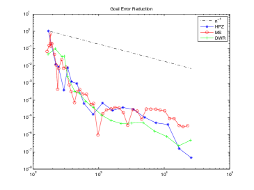
Here, we also manipulate ω𝜔\omega, the frequency of the sinusoid in the primal problem. We observe that varying the structure of the problem changes the relative efficiency of the three algorithms.

The goal function is given by

g(x,y)=aexp(a((xx0)2+(yy0)2))+aexp(a((xx1)2+(yy1)2)),𝑔𝑥𝑦𝑎𝑎superscript𝑥subscript𝑥02superscript𝑦subscript𝑦02𝑎𝑎superscript𝑥subscript𝑥12superscript𝑦subscript𝑦12\displaystyle g(x,y)=a\exp(-a((x-x_{0})^{2}+(y-y_{0})^{2}))+a\exp(-a((x-x_{1})^{2}+(y-y_{1})^{2})),

with a=400𝑎400a=400 and (x0,y0)=(0.7,0.7)subscript𝑥0subscript𝑦00.70.7(x_{0},y_{0})=(0.7,0.7).

The data f(x,y)𝑓𝑥𝑦f(x,y) is chosen so the exact solution u(x,y)𝑢𝑥𝑦u(x,y) is given by

u=sin(ωπx)sin(ωπy)12[(xxp)2+(yyp)2]+103 with (xp,yp)=(0.3,0.3).𝑢𝜔𝜋𝑥𝜔𝜋𝑦12delimited-[]superscript𝑥subscript𝑥𝑝2superscript𝑦subscript𝑦𝑝2superscript103 with subscript𝑥𝑝subscript𝑦𝑝0.30.3u=\sin(\omega\pi x)\sin(\omega\pi y)\frac{1}{2[(x-x_{p})^{2}+(y-y_{p})^{2}]+10^{-3}}~{}\text{ with }~{}(x_{p},y_{p})=(0.3,0.3).
(6.5) Figure4𝐹𝑖𝑔𝑢𝑟𝑒4\displaystyle Figure~{}\ref{fig:HSD_xy73} (x1,y1)=(0.7,0.3)subscript𝑥1subscript𝑦10.70.3\displaystyle(x_{1},y_{1})=(0.7,0.3) ω=1,𝜔1\displaystyle\omega=1,
(6.6) (x1,y1)=(0.7,0.3)subscript𝑥1subscript𝑦10.70.3\displaystyle(x_{1},y_{1})=(0.7,0.3) ω=2.𝜔2\displaystyle\omega=2.
(6.7) Figure6𝐹𝑖𝑔𝑢𝑟𝑒6\displaystyle Figure~{}\ref{fig:HSD_xy53} (x1,y1)=(0.55,0.3)subscript𝑥1subscript𝑦10.550.3\displaystyle(x_{1},y_{1})=(0.55,0.3) ω=1,𝜔1\displaystyle\omega=1,
(6.8) (x1,y1)=(0.55,0.3)subscript𝑥1subscript𝑦10.550.3\displaystyle(x_{1},y_{1})=(0.55,0.3) ω=2.𝜔2\displaystyle\omega=2.
(6.9) Figure7𝐹𝑖𝑔𝑢𝑟𝑒7\displaystyle Figure~{}\ref{fig:HSD_xy43} (x1,y1)=(0.4,0.3)subscript𝑥1subscript𝑦10.40.3\displaystyle(x_{1},y_{1})=(0.4,0.3) ω=1,𝜔1\displaystyle\omega=1,
(6.10) (x1,y1)=(0.4,0.3)subscript𝑥1subscript𝑦10.40.3\displaystyle(x_{1},y_{1})=(0.4,0.3) ω=2.𝜔2\displaystyle\omega=2.

Compared to parameter sets (6.1)-(6.4), DWR generally fares as well or better than the residual based methods for (6.5)-(6.10).
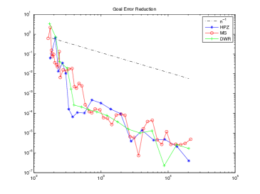
Refer to caption
Refer to caption
Figure 4. Left: goal error after 19 HPZ, 46 MS and 19 DWR iterations for  (6.5). Right: goal error after 20 HPZ, 47 MS and 18 DWR iterations for  (6.6), compared with n1superscript𝑛1n^{-1}

.

Refer to caption
Refer to caption
Refer to caption
Figure 5. Left: 13 iterations of HPZ (1187 elements). Center: 26 iterations of MS (1156) elements). Right: 14 iterations of DWR (1115 elements) for  (6.5).

For the parameter sets (6.5) and (6.6) shown in Figure 4 both dual spikes are remote from the primal data. As seen in Figure 5 each algorithm displays a distinct trend in its adaptive refinement: HPZ refines for both primal and dual; MS refines for both with a bias towards the primal, with 17 primal refinements and 10 dual refinements in this case; DWR refines with a bias towards the dual data. When ω=1𝜔1\omega=1, HPZ and DWR show similar goal error reduction while MS stalls at least on these relatively early refinements. For ω=2𝜔2\omega=2, MS still shows a slight tendency to refine more for the primal than the dual; however the error reductions is generally similar to the other two methods.
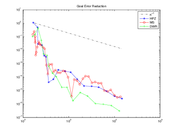
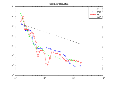
Refer to caption
Refer to caption
Figure 6. Left: goal error after 19 HPZ, 44 MS and 19 DWR iterations for  (6.7). Right: goal error after 20 HPZ, 46 MS and 19 DWR iterations for  (6.8), compared with n1superscript𝑛1n^{-1}.

Figure 6 shows the performance of the algorithms for parameter sets (6.7) and (6.8). Here, the residual methods are similar and both outperformed by DWR in the case ω=1𝜔1\omega=1 while all three methods are similar in the case ω=2𝜔2\omega=2, with HPZ showing a trend towards slightly greater goal error reduction.
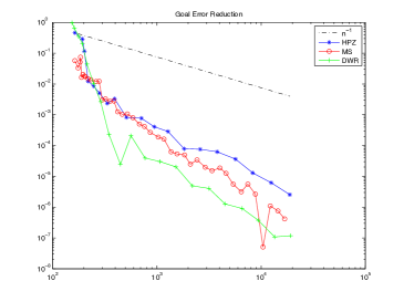
Refer to caption
Refer to caption
Figure 7. Left: goal error after 20 HP, 45 MS and 21 DWR iterations for  (6.9). Right: goal error after 18 HP, 40 MS and 18 DWR iterations for  (6.10), compared with n1superscript𝑛1n^{-1}.

Finally, Figure 7 shows the performance of these methods for parameter sets (6.9) and (6.10). In these examples, DWR outperforms the residual based methods. In these two cases, the spikes in primal data and dual solution have an isolated area of overlap that coincides with the spikes in the primal solution and dual data, the situation that makes the DWR method the most efficient (cf. [25]). Varying the frequency of the primal data again changes the relative efficiencies of the residual based methods. In contrast to (6.5) and (6.6), the performance of MS decreases when the frequency ω𝜔\omega increases from 111 to 222.

The effectiveness of the DWR method is based on the assumption that R(uh),zh𝑅subscript𝑢subscript𝑧\langle R(u_{h}),z_{h}\rangle is a good predictor for the error g(eh)𝑔subscript𝑒g(e_{h}). This appears to work so long as rapidly changing gradients in the dual solution coincide spatially with spikes in g(x,y)𝑔𝑥𝑦g(x,y), and the primal residual R(uh)𝑅subscript𝑢R(u_{h}) captures sufficient information about the primal solution in the vicinity of the influence function zhsubscript𝑧z_{h}. For an example of where the first condition fails, we refer to the linear convection-diffusion problem discussed in [25], and a demonstration of the second condition is (6.1). Under certain conditions, namely a confined region where the spikes in primal data and dual solution overlap that coincides with the overlap in the spikes in the primal solution and dual data, the DWR methods outperforms the residual based methods.

In many cases, all three methods display similar performance, yet with qualitatively different adaptive mesh refinements. The relative performances of HPZ and MS do appear to be dependent on the structure of the primal problem, however it is not clear at this stage how to predict which algorithm will yield a better reduction in goal error. In problems where the HPZ and MS results appear similar, we note that MS takes considerably longer to run as it may require approximately twice as many total iterations of the algorithm where most of the runtime is spent on nonlinear solves. We further emphasize that the results here consider the error vs. mesh cardinality, not total degrees of freedom. It is of further interest to compare the performance of DWR with the residual based methods using higher order finite elements for the dual and possibly primal problems. Determining classes of problems for which each method is best suited is currently under investigation by the present authors.

7. Conclusion

In this article we developed convergence theory for a class of goal-oriented adaptive finite element algorithms for second order semilinear elliptic equations. We first introduced several approximate dual problems, and briefly discussed the target problem class. We then reviewed some standard facts concerning conforming finite element discretization and error-estimate-driven adaptive finite element methods (AFEM). We included a brief summary of a priori estimates for semilinear problems, and then described goal-oriented variations of the standard approach to AFEM (GOAFEM). Following the recent work of Mommer-Stevenson and Holst-Pollock for linear problems, we established contraction of GOAFEM for the primal problem. We also developed some additional estimates that make it possible to establish contraction of the combined quasi-error, and showed convergence in the sense of the quantity of interest. Some simple numerical experiments confirmed these theoretical predictions and demonstrated that our method performs comparably to other standard adaptive goal-oriented strategies, and has the additional advantage of provable convergence for problems where the theory has not been developed for the other two methods. Our analysis was based on the recent contraction frameworks for the semilinear problem developed by Holst, Tsogtgerel, and Zhu and Bank, Holst, Szypowski and Zhu and those for linear problems as in Cascon, Kreuzer, Nochetto and Siebert, and Nochetto, Siebert, and Veeser. In addressing the goal-oriented problem we based our approach on that of Mommer and Stevenson for symmetric linear problems and Holst and Pollock for nonsymmetric problems. However, unlike the linear case, we were faced with tracking linearized and approximate dual sequences in order to establish contraction with respect to the quantity of interest.

In the present paper we assume the primal and approximate dual solutions are solved on the same mesh at each iteration. The determination of strong convergence results for a method which solves the primal (nonlinear) problem on a coarse mesh and the dual on a fine mesh is the subject of future investigation.

Acknowledgments

MH was supported in part by NSF Awards 1065972, 1217175, 1262982, 1318480, and by AFOSR Award FA9550-12-1-0046. SP and YZ were supported in part by NSF Awards 1065972 and 1217175. YZ was also supported in part by NSF DMS 1319110, and in part by University Research Committee Grant No. F119 at Idaho State University, Pocatello, Idaho.

References

  • [1] O. Axelsson and V. A. Barker. Finite element solution of boundary value problems: theory and computation. Society for Industrial and Applied Mathematics, Philadelphia, PA, USA, 2001.
  • [2] W. Bangerth and R. Rannacher. Adaptive finite element methods for differential equations. Birkhauser, Boston, 2003.
  • [3] R. Bank, M. Holst, R. Szypowski, and Y. Zhu. Convergence of AFEM for semilinear problems with inexact solvers, 2011.
  • [4] R. Bank, M. Holst, R. Szypowski, and Y. Zhu. Finite element error estimates for critical growth semilinear problems without angle conditions, 2011.
  • [5] R. Becker and R. Rannacher. A feed-back approach to error control in finite element methods: Basic analysis and examples. East-West Journal of Numerical Mathematics, 4:237–264, 1996.
  • [6] R. Becker and R. Rannacher. Weighted a posteriori error control in FE methods. Preprint 96-1, SFB 359, Universitat, pages 18–22, 1996.
  • [7] R. Becker and R. Rannacher. An optimal control approach to a posteriori error estimation in finite element methods. Acta Numerica, pages 1–102, 2001.
  • [8] P. Binev, W. Dahmen, and R. DeVore. Adaptive finite element methods with convergence rates. Numer. Math., 97(2):219–268, 2004.
  • [9] S. Brenner and L. Scott. The Mathematical Theory of Finite Element Methods. Springer-Verlag, third edition, 2008.
  • [10] J. M. Cascon, C. Kreuzer, R. H. Nochetto, and K. G. Siebert. Quasi-optimal convergence rate for an adaptive finite element method. SIAM J. Numer. Anal., 46(5):2524–2550, 2008.
  • [11] P. G. Ciarlet. Finite Element Method for Elliptic Problems. Society for Industrial and Applied Mathematics, Philadelphia, PA, USA, 2002.
  • [12] W. Dahmen, A. Kunoth, and J. Vorloeper. Convergence of Adaptive Wavelet Methods for Goal-oriented Error Estimation. Sonderforschungsbereich 611, Singuläre Phänomene und Skalierung in Mathematischen Modellen. SFB 611, 2006.
  • [13] W. Dörfler. A convergent adaptive algorithm for Poisson’s equation. SIAM Journal on Numerical Analysis, 33:1106–1124, 1996.
  • [14] K. Eriksson, D. Estep, P. Hansbo, and C. Johnson. Introduction to adaptive methods for differential equations. Acta Numerica, pages 105–158, 1995.
  • [15] D. Estep, M. Holst, and M. Larson. Generalized green’s functions and the effective domain of influence. SIAM J. Sci. Comput, 26:1314–1339, 2002.
  • [16] D. Estep, M. Holst, and D. Mikulencak. Accounting for stability: A posteriori error estimates based on residuals and variational analysis. In Communications in Numerical Methods in Engineering, pages 200–2, 2001.
  • [17] D. Estep, M. G. Larson, and R. D. Williams. Estimating the error of numerical solutions of systems of reaction-diffusion equations. Mem. Amer. Math. Soc., 146(696):101–109, 2000.
  • [18] L. C. Evans. Partial Differential Equations (Graduate Studies in Mathematics, V. 19) GSM/19. American Mathematical Society, 1998.
  • [19] D. Gilbarg and N. S. Trudinger. Elliptic partial differential equations of second order. Springer-Verlag, 1977.
  • [20] M. Giles and E. Süli. Adjoint methods for PDEs: a posteriori error analysis and postprocessing by duality. Acta Numerica, 11:145–236, 2003.
  • [21] T. Grätsch and K.-J. Bathe. A posteriori error estimation techniques in practical finite element analysis. Computers & Structures, 83(4-5):235 – 265, 2005.
  • [22] M. Holst. Adaptive numerical treatment of elliptic systems on manifolds. Adv. Comput. Math., 15(1–4):139–191, 2001. Available as arXiv:1001.1367 [math.NA].
  • [23] M. Holst. Applications of domain decomposition and partition of unity methods in physics and geometry. In I. Herrera, D. Keyes, O. Widlund, and R. Yates, editors, Proceedings of the Fourteenth International Conference on Domain Decomposition Methods, pages 63–78. National Autonomous University of Mexico (UNAM), 2003. Available as arXiv:1001.1364 [math.NA].
  • [24] M. Holst, J. McCammon, Z. Yu, Y. Zhou, and Y. Zhu. Adaptive finite element modeling techniques for the Poisson-Boltzmann equation. Communications in Computational Physics, 11(1):179–214, 2012. Available as arXiv:1009.6034 [math.NA].
  • [25] M. Holst and S. Pollock. Convergence of goal oriented methods for nonsymmetric problems, 2011.
  • [26] M. Holst, R. Szypowski, and Y. Zhu. Adaptive finite element methods with inexact solvers for the nonlinear poisson-boltzmann equation. In R. Bank, M. Holst, O. Widlund, and J. Xu, editors, Domain Decomposition Methods in Science and Engineering XX, volume 91 of Lecture Notes in Computational Science and Engineering, pages 167–174. Springer Berlin Heidelberg, 2013.
  • [27] M. Holst, R. Szypowski, and Y. Zhu. Two-grid methods for semilinear interface problems. Numerical Methods for Partial Differential Equations, 29(5):1729–1748, 2013.
  • [28] M. Holst, G. Tsogtgerel, and Y. Zhu. Local and global convergence of adaptive methods for nonlinear partial differential equations, 2008.
  • [29] A. Jüngel and A. Unterreiter. Discrete minimum and maximum principles for finite element approximations of non-monotone elliptic equations. Numer. Math., 99(3):485–508, 2005.
  • [30] J. Karatson and S. Korotov. Discrete maximum principles for finite element solutions of nonlinear elliptic problems with mixed boundary conditions. Numerische Mathematik, 99:669–698, 2005.
  • [31] T. Kerkhoven and J. W. Jerome. Lsubscript𝐿L_{\infty} stability of finite element approximations of elliptic gradient equations. Numerische Mathematik, 57:561–575, 1990.
  • [32] S. Kesavan. Topics in Functional Analysis and Applications. John Wiley and Sons, Inc., New York, NY, 1989.
  • [33] S. Korotov. A posteriori error estimation of goal-oriented quantities for elliptic type bvps. Journal of Computational and Applied Mathematics, 191(2):216 – 227, 2006.
  • [34] K. Mekchay and R. Nochetto. Convergence of adaptive finite element methods for general second order linear elliptic PDE. SINUM, 43(5):1803–1827, 2005.
  • [35] M. S. Mommer and R. Stevenson. A goal-oriented adaptive finite element method with convergence rates. SIAM J. Numer. Anal., 47(2):861–886, 2009.
  • [36] K.-S. Moon, E. von Schwerin, A. Szepessy, and R. Tempone. Convergence rates for an adaptive dual weighted residual finite element algorithm. BIT, 46(2):367–407, 2006.
  • [37] R. H. Nochetto, K. G. Siebert, and A. Veeser. Theory of adaptive finite element methods: an introduction, pages 409 – 542. Springer, 2009.
  • [38] J. Oden and S. Prudhomme. Goal-oriented error estimation and adaptivity for the finite element method. Computers and Mathematics with Applications, 41:735–756, 2001.
  • [39] E. G. Sewell. Automatic generation of triangulations for piecewise polynomial approximation. In Ph. D. dissertation. Purdue Univ., West Lafayette, Ind., 1972.
  • [40] G. Strang and G. J. Fix. An Analysis of the Finite Element Method. Prentice-Hall (Series in Automatic Computation), Englewood Cliffs, N. J., 1973.
  • [41] M. Struwe. Variational Methods. Springer-Verlag, Berlin, Germany, 3 edition, 2000.
  • [42] R. Verfürth. A posteriori error estimates for nonlinear problems. finite element discretizations of elliptic equations. Mathematics of Computation, 62(206):445–475, Apr. 1994.
  • [43] R. Verfürth. A review of a posteriori error estimation and adaptive mesh refinement tecniques. B. G. Teubner, 1996.