Bayesian Nonparametric Hidden Semi-Markov Models

Abstract

There is much interest in the Hierarchical Dirichlet Process Hidden Markov Model (HDP-HMM) as a natural Bayesian nonparametric extension of the ubiquitous Hidden Markov Model for learning from sequential and time-series data. However, in many settings the HDP-HMM’s strict Markovian constraints are undesirable, particularly if we wish to learn or encode non-geometric state durations. We can extend the HDP-HMM to capture such structure by drawing upon explicit-duration semi-Markov modeling, which has been developed mainly in the parametric non-Bayesian setting, to allow construction of highly interpretable models that admit natural prior information on state durations.

In this paper we introduce the explicit-duration Hierarchical Dirichlet Process Hidden semi-Markov Model (HDP-HSMM) and develop sampling algorithms for efficient posterior inference. The methods we introduce also provide new methods for sampling inference in the finite Bayesian HSMM. Our modular Gibbs sampling methods can be embedded in samplers for larger hierarchical Bayesian models, adding semi-Markov chain modeling as another tool in the Bayesian inference toolbox. We demonstrate the utility of the HDP-HSMM and our inference methods on both synthetic and real experiments.

Keywords: Bayesian nonparametrics, time series, semi-Markov, sampling algorithms, Hierarchical Dirichlet Process Hidden Markov Model

1 Introduction

Given a set of sequential data in an unsupervised setting, we often aim to infer meaningful states, or “topics,” present in the data along with characteristics that describe and distinguish those states. For example, in a speaker diarization (or who-spoke-when) problem, we are given a single audio recording of a meeting and wish to infer the number of speakers present, when they speak, and some characteristics governing their speech patterns (Tranter and Reynolds, 2006; Fox et al., 2008). Or in separating a home power signal into the power signals of individual devices, we would be able to perform the task much better if we were able to exploit our prior knowledge about the levels and durations of each device’s power modes (Kolter and Johnson, 2011). Such learning problems for sequential data are pervasive, and so we would like to build general models that are both flexible enough to be applicable to many domains and expressive enough to encode the appropriate information.

Hidden Markov Models (HMMs) have proven to be excellent general models for approaching learning problems in sequential data, but they have two significant disadvantages: (1) state duration distributions are necessarily restricted to a geometric form that is not appropriate for many real-world data, and (2) the number of hidden states must be set a priori so that model complexity is not inferred from data in a Bayesian way.

Recent work in Bayesian nonparametrics has addressed the latter issue. In particular, the Hierarchical Dirichlet Process HMM (HDP-HMM) has provided a powerful framework for inferring arbitrarily large state complexity from data (Teh et al., 2006; Beal et al., 2002). However, the HDP-HMM does not address the issue of non-Markovianity in real data. The Markovian disadvantage is even compounded in the nonparametric setting, since non-Markovian behavior in data can lead to the creation of unnecessary extra states and unrealistically rapid switching dynamics (Fox et al., 2008).

One approach to avoiding the rapid-switching problem is the Sticky HDP-HMM (Fox et al., 2008), which introduces a learned global self-transition bias to discourage rapid switching. Indeed, the Sticky model has demonstrated significant performance improvements over the HDP-HMM for several applications. However, it shares the HDP-HMM’s restriction to geometric state durations, thus limiting the model’s expressiveness regarding duration structure. Moreover, its global self-transition bias is shared among all states, and so it does not allow for learning state-specific duration information. The infinite Hierarchical HMM (Heller et al., 2009) induces non-Markovian state durations at the coarser levels of its state hierarchy, but even the coarser levels are constrained to have a sum-of-geometrics form, and hence it can be difficult to incorporate prior information. Furthermore, constructing posterior samples from any of these models can be computationally expensive, and finding efficient algorithms to exploit problem structure is an important area of research.

These potential limitations and needed improvements to the HDP-HMM motivate this investigation into explicit-duration semi-Markov modeling, which has a history of success in the parametric (and usually non-Bayesian) setting. We combine semi-Markovian ideas with the HDP-HMM to construct a general class of models that allow for both Bayesian nonparametric inference of state complexity as well as general duration distributions. In addition, the sampling techniques we develop for the Hierarchical Dirichlet Process Hidden semi-Markov Model (HDP-HSMM) provide new approaches to inference in HDP-HMMs that can avoid some of the difficulties which result in slow mixing rates. We demonstrate the applicability of our models and algorithms on both synthetic and real datasets.

The remainder of this paper is organized as follows. In Section 2, we describe explicit-duration HSMMs and existing HSMM message-passing algorithms, which we use to build efficient Bayesian inference algorithms. We also provide a brief treatment of the Bayesian nonparametric HDP-HMM and sampling inference algorithms. In Section 3 we develop the HDP-HSMM and related models. In Section 4 we develop extensions of the weak-limit and direct assignment samplers (Teh et al., 2006) for the HDP-HMM to our models and describe some techniques for improving the computational efficiency in some settings.

Section 5 demonstrates the effectiveness of the HDP-HSMM on both synthetic and real data. In synthetic experiments, we demonstrate that our sampler mixes very quickly on data generated by both HMMs and HSMMs and accurately learns parameter values and state cardinality. We also show that while an HDP-HMM is unable to capture the statistics of an HSMM-generated sequence, we can build HDP-HSMMs that efficiently learn whether data were generated by an HMM or HSMM. As a real-data experiment, we apply the HDP-HSMM to a problem in power signal disaggregation.

2 Background and Notation

In this section, we outline three main background topics: our notation for Bayesian HMMs, conventions for explicit-duration HSMMs, and the Bayesian nonparametric HDP-HMM.

2.1 HMMs

2.1.1 Basic Notation

The core of the HMM consists of two layers: a layer of hidden state variables and a layer of observation or emission variables, as shown in Figure 1. The hidden state sequence, $x=(x_{t})_{t=1}^{T}$, is a sequence of random variables on a finite alphabet, i.e. $x_{t}\in\{1,2,\ldots,N\}$, that form a Markov chain. In this paper, we focus on time-homogeneous models, in which the transition distribution does not depend on $t$. The transition parameters are collected into a row-stochastic transition matrix $\pi=(\pi_{ij})_{i,j=1}^{N}$ where $\pi_{ij}=p(x_{t+1}=j|x_{t}=i)$. We also use $\{\pi_{i}\}$ to refer to the set of rows of the transition matrix. We use $p(y_{t}|x_{t},\{\theta_{i}\})$ to denote the emission distribution, where $\{\theta_{i}\}$ represents parameters.

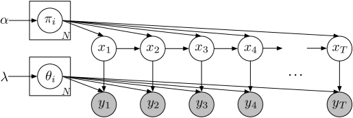
Figure 1: Basic graphical model for the Bayesian HMM. Parameters for the transition, emission, and initial state distributions are random variables. The symbol $\alpha$ represents the hyperparameter for the prior distributions on state-transition parameters. The shaded nodes indicate observations on which we condition to form the posterior distribution over the unshaded latent components.

The Bayesian approach allows us to model uncertainty over the parameters and perform model averaging (e.g. forming a prediction of an observation $y_{T+1}$ by integrating out all possible parameters and state sequences), generally at the expense of somewhat more expensive algorithms. This paper is concerned with the Bayesian approach and so the model parameters are treated as random variables, with their priors denoted $p(\pi|\alpha)$ and $p(\{\theta_{i}\}|H)$.

2.2 HSMMs

There are several approaches to hidden semi-Markov models (Murphy, 2002; Yu, 2010). We focus on explicit duration semi-Markov modeling; i.e., we are interested in the setting where each state’s duration is given an explicit distribution. Such HSMMs are generally treated from a non-Bayesian perspective in the literature, where parameters are estimated and fixed via an approximate maximum-likelihood procedure (particularly the natural Expectation-Maximization algorithm, which constitutes a local search).

The basic idea underlying this HSMM formalism is to augment the generative process of a standard HMM with a random state duration time, drawn from some state-specific distribution when the state is entered. The state remains constant until the duration expires, at which point there is a Markov transition to a new state. We use the random variable $D_{t}$ to denote the duration of a state that is entered at time $t$, and we write the probability mass function for the random variable as $p(d_{t}|x_{t}=i)$.

A graphical model for the explicit-duration HSMM is shown in Figure 2 (from (Murphy, 2002)), though the number of nodes in the graphical model is itself random. In this picture, we see there is a Markov chain (without self-transitions) on $S$ “super-state” nodes, $(z_{s})_{s=1}^{S}$, and these super-states in turn emit random-length segments of observations, of which we observe the first $T$. Here, the symbol $D_{s}$ is used to denote the random length of the observation segment of super-state $s$ for $s=1,\ldots,S$. The “super-state” picture separates the Markovian transitions from the segment durations.

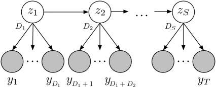
Figure 2: HSMM interpreted as a Markov chain on a set of super-states, $(z_{s})_{s=1}^{S}$. The number of shaded nodes associated with each $z_{s}$, denoted by $D_{s}$, is drawn from a state-specific duration distribution.

When defining an HSMM model, one must also choose whether the observation sequence ends exactly on a segment boundary or whether the observations are censored at the end, so that the final segment may possibly be cut off in the observations. We focus on the right-censored formulation in this paper, but our models and algorithms can easily be modified to the uncensored or left-censored cases. For a further discussion, see (Guédon, 2007).

It is possible to perform efficient message-passing inference along an HSMM state chain (conditioned on parameters and observations) in a way similar to the standard alpha-beta dynamic programming algorithm for standard HMMs. The “backwards” messages are crucial in the development of efficient sampling inference in Section 4 because the message values can be used to efficiently compute the posterior information necessary to block-sample the hidden state sequence $(x_{t})$, and so we briefly describe the relevant part of the existing HSMM message-passing algorithm. As derived in (Murphy, 2002), we can define and compute the backwards messages $B$ and $B^{*}$ as follows:

$$B_{t}(i) \mathrel{\mathop{\mathchar 58\relax}}=p(y_{t+1\mathrel{\mathop{\mathchar 58\relax}}T}|x_{t}=i,F_{t}=1)$$ (1)

$$=\sum_{j}B_{t}^{*}(j)p(x_{t+1}=j|x_{t}=i)$$ (2)

$$B_{t}^{*}(i) \mathrel{\mathop{\mathchar 58\relax}}=p(y_{t+1\mathrel{\mathop{\mathchar 58\relax}}T}|x_{t+1}=i,F_{t}=1)$$ (3)

$$=\sum_{d=1}^{T-t}B_{t+d}(i)\underbrace{p(D_{t+1}=d|x_{t+1}=i)}_{\text{duration prior term}}\cdot\underbrace{p(y_{t+1\mathrel{\mathop{\mathchar 58\relax}}t+d}|x_{t+1}=i,D_{t+1}=d)}_{\text{likelihood term}}$$ (4)

$$\quad+\underbrace{p(D_{t+1}>T-t|x_{t+1}=i)p(y_{t+1\mathrel{\mathop{\mathchar 58\relax}}T}|x_{t+1}=i,D_{t+1}>T-t)}_{\text{censoring term}}$$ (5)

$$B_{T}(i) \mathrel{\mathop{\mathchar 58\relax}}=1$$ (6)

where we have split the messages into $B$ and $B^{*}$ components for convenience and used $y_{k_{1}\mathrel{\mathop{\mathchar 58\relax}}k_{2}}$ to denote $(y_{k_{1}},\ldots,y_{k_{2}})$. $D_{t+1}$ represents the duration of the segment beginning at time $t+1$. The conditioning on the parameters of the distributions, namely the observation, duration, and transition parameters, is suppressed from the notation.

We write $F_{t}=1$ to indicate a new segment begins at $t+1$ (Murphy, 2002), and so to compute the message from $t+1$ to $t$ we sum over all possible lengths $d$ for the segment beginning at $t+1$, using the backwards message at $t+d$ to provide aggregate future information given a boundary just after $t+d$. The final additive term in the expression for $B_{t}^{*}(i)$ is described in (Guédon, 2007); it constitutes the contribution of state segments that run off the end of the provided observations, as per the censoring assumption, and depends on the survival function of the duration distribution.

Though a very similar message-passing subroutine is used in HMM Gibbs samplers, there are significant differences in computational cost between the HMM and HSMM message computations. The greater expressive power of the HSMM model necessarily increases the computational cost: the above message passing requires $\mathcal{O}(T^{2}N+TN^{2})$ basic operations for a chain of length $T$ and state cardinality $N$, while the corresponding HMM message passing algorithm requires only $\mathcal{O}(TN^{2})$. However, if the support of the duration distribution is limited, or if we truncate possible segment lengths included in the inference messages to some maximum $d_{\text{max}}$, we can instead express the asymptotic message passing cost as $\mathcal{O}(Td_{\text{max}}N+TN^{2})$. Such truncations are often natural as the duration prior often causes the message contributions to decay rapidly with sufficiently large $d$. Though the increased complexity of message-passing over an HMM significantly increases the cost per iteration of sampling inference for a global model, the cost is offset because HSMM samplers need far fewer total iterations to converge. See the experiments in Section 5.

2.3 The HDP-HMM and Sticky HDP-HMM

The HDP-HMM (Teh et al., 2006) provides a natural Bayesian nonparametric treatment of the classical Hidden Markov Model. The model employs an HDP prior over an infinite state space, which enables both inference of state complexity and Bayesian mixing over models of varying complexity. We provide a brief overview of the HDP-HMM model and relevant inference algorithms, which we extend to develop the HDP-HSMM. A much more thorough treatment of the HDP-HMM can be found in, for example, (Fox, 2009).

The generative process $\text{HDP-HMM}(\gamma,\alpha,H)$ given concentration parameters $\gamma,\alpha>0$ and base measure (observation prior) $H$ can be summarized as:

$$\beta \sim\text{GEM}(\gamma)$$ (7)

$$\pi_{i} \stackrel{{\scriptstyle\text{iid}}}{{\sim}}\text{DP}(\alpha,\beta) \theta_{i}\stackrel{{\scriptstyle\text{iid}}}{{\sim}}H i=1,2,\ldots$$ (8)

$$x_{t} \sim\pi_{x_{t-1}}$$ (9)

$$y_{t} \sim f(\theta_{x_{t}}) t=1,2,\ldots,T$$ (10)

where GEM denotes a stick breaking process (Sethuraman., 1994) and $f$ denotes an observation distribution parameterized by draws from $H$. We set $x_{1}\mathrel{\mathop{\mathchar 58\relax}}=1$. We have also suppressed explicit conditioning from the notation. See Figure 3 for a graphical model.

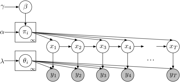
Figure 3: Graphical model for the HDP-HMM.

The HDP plays the role of a prior over infinite transition matrices: each $\pi_{j}$ is a DP draw and is interpreted as the transition distribution from state $j$, i.e. the $j$th row of the infinite transition matrix. The $\pi_{j}$ are linked by being DP draws parameterized by the same discrete measure $\beta$, thus $\mathbb{E}[\pi_{j}]=\beta$ and the transition distributions tend to have their mass concentrated around a typical set of states, providing the desired bias towards re-entering and re-using a consistent set of states.

The Chinese Restaurant Franchise and direct-assignment collapsed sampling methods described in (Teh et al., 2006; Fox, 2009) are approximate inference algorithms for the full infinite dimensional HDP, but they have a particular weakness in the sequential-data context of the HDP-HMM: each state transition must be re-sampled individually, and strong correlations within the state sequence significantly reduce mixing rates(Fox, 2009). As a result, finite approximations to the HDP have been studied for the purpose of providing faster mixing. Of particular note is the popular weak limit approximation, used in (Fox et al., 2008), which has been shown to reduce mixing times for HDP-HMM inference while sacrificing little of the “tail” of the infinite transition matrix. In this paper, we describe how the HDP-HSMM with geometric durations can provide an HDP-HMM sampling inference algorithm that maintains the “full” infinite-dimensional sampling process while mitigating the detrimental mixing effects due to the strong correlations in the state sequence, thus providing a new alternative to existing HDP-HMM sampling methods.

The Sticky HDP-HMM augments the HDP-HMM with an extra parameter $\kappa>0$ that biases the process towards self-transitions and thus provides a method to encourage longer state durations. The $\text{Sticky-HDP-HMM}(\gamma,\alpha,\kappa,H)$ generative process can be written

$$\beta \sim\text{GEM}(\gamma)$$ (11)

$$\pi_{i} \stackrel{{\scriptstyle\text{iid}}}{{\sim}}\text{DP}(\alpha+\kappa,\beta+\kappa\delta_{j}) \theta_{i}\stackrel{{\scriptstyle\text{iid}}}{{\sim}}H i=1,2,\ldots$$ (12)

$$x_{t} \sim\pi_{x_{t-1}}$$ (13)

$$y_{t} \sim f(\theta_{x_{t}}) t=1,2,\ldots,T$$ (14)

where $\delta_{j}$ denotes an indicator function that takes value $1$ at index $j$ and $0$ elsewhere. While the Sticky HDP-HMM allows some control over duration statistics, the state duration distributions remain geometric; the goal of this work is to provide a model in which any duration distributions may be used.

3 Models

In this section, we introduce the explicit-duration HSMM-based models that we use in the remainder of the paper. We define the finite Bayesian HSMM and the HDP-HSMM and show how they can be used as components in more complex models, such as in a factorial structure. We describe generative processes that do not allow self-transitions in the state sequence, but we emphasize that we can also allow self-transitions and still employ the inference algorithms we describe; in fact, allowing self-transitions simplifies inference in the HDP-HSMM, since complications arise as a result of the hierarchical prior and an elimination of self-transitions. However, there is a clear modeling gain by eliminating self-transitions: when self-transitions are allowed, the “explicit duration distributions” do not model the state duration statistics directly. To allow direct modeling of state durations, we must consider the case where self-transitions do not occurr.

We do not investigate here the problem of selecting particular observation and duration distribution classes; model selection is a fundamental challenge in generative modeling, and models must be chosen to capture structure in any particular data. Instead, we provide the HDP-HSMM and related models as tools in which modeling choices (such as the selection of observation and duration distribution classes to fit particular data) can be made flexibly and naturally.

3.1 Finite Bayesian HSMM

The finite Bayesian HSMM is a combination of the Bayesian HMM approach with semi-Markov state durations and is the model we generalize to the HDP-HSMM. Some forms of finite Bayesian HSMMs have been described previously, such as in (Hashimoto et al., 2009) which treats observation parameters as Bayesian latent variables, but to the best of our knowledge the first fully Bayesian treatment of all latent components of the HSMM was given in (Johnson and Willsky, 2010) and later independently in (Dewar et al., 2012), which allows self-transitions.

It is instructive to compare this construction with that of the finite model used in the weak-limit HDP-HSMM sampler that will be described in Section 4.2, since in that case the hierarchical ties between rows of the transition matrix requires particular care.

The generative process for a Bayesian HSMM with $N$ states and observation and duration parameter prior distributions of $H$ and $G$, respectively, can be summarized as

$$\pi_{i} \stackrel{{\scriptstyle\text{iid}}}{{\sim}}\text{Dir}(\alpha(1-\delta_{i})) (\theta_{i},\omega_{i})\stackrel{{\scriptstyle\text{iid}}}{{\sim}}H\times G i=1,2,\ldots,N$$ (15)

$$z_{s} \sim\pi_{z_{s-1}}$$ (16)

$$D_{s} \sim g(\omega_{z_{s}}) s=1,2,\ldots$$ (17)

$$x_{t_{s}^{1}\mathrel{\mathop{\mathchar 58\relax}}t_{s}^{2}} =z_{s}$$ (18)

$$y_{t_{s}^{1}\mathrel{\mathop{\mathchar 58\relax}}t_{s}^{2}} \stackrel{{\scriptstyle\text{iid}}}{{\sim}}f(\theta_{z_{s}}) t_{s}^{1}=\sum_{\bar{s}<s}D_{\bar{s}} t_{s}^{2}=t_{s}^{1}+D_{s}-1$$ (19)

where $f$ and $g$ denote observation and duration distributions parameterized by draws from $H$ and $G$, respectively. The indices $t_{s}^{1}$ and $t_{s}^{2}$ denote the first and last index of segment $s$, respectively, and $x_{t_{s}^{1}\mathrel{\mathop{\mathchar 58\relax}}t_{s}^{2}}\mathrel{\mathop{\mathchar 58\relax}}=(x_{t_{s}^{1}},x_{t_{s}^{1}+1},\ldots,x_{t_{s}^{2}})$. We use $\text{Dir}(\alpha(1-\delta_{i}))$ to denote a symmetric Dirichlet distribution with parameter $\alpha$ except with the $i$th component of the hyperparameter vector set to zero, hence fixing $\pi_{ii}=0$ and ensuring there will be no self-transitions sampled in the super-state sequence $(z_{s})$. We also define the label sequence $(x_{t})$ for convenience; the pair $(z_{s},D_{s})$ is the run-length encoding of $(x_{t})$. The process as written generates an infinite sequence of observations; we observe a finite prefix of size $T$.

Note, crucially, that in this definition the $\pi_{i}$ are not tied across various $i$. In the HDP-HSMM, as well as the weak limit model used for approximate inference in the HDP-HSMM, the $\pi_{i}$ will be tied through the hierarchical prior (specifically via $\beta$), and that connection is necessary to penalize the total number of states and encourage a small, consistent set of states to be visited in the state sequence. However, the interaction between the hierarchical prior and the elimination of self-transitions present an inference challenge.

3.2 HDP-HSMM

The generative process of the HDP-HSMM is similar to that of the HDP-HMM (as described in, e.g., (Fox et al., 2008)), with some extra work to include duration distributions. The process $\text{HDP-HSMM}(\gamma,\alpha,H,G)$, illustrated in Figure 4, can be written

$$\beta \sim\text{GEM}(\gamma)$$ (20)

$$\pi_{i} \stackrel{{\scriptstyle\text{iid}}}{{\sim}}\text{DP}(\alpha,\beta) (\theta_{i},\omega_{i})\stackrel{{\scriptstyle\text{iid}}}{{\sim}}H\times G i=1,2,\ldots$$ (21)

$$z_{s} \sim\bar{\pi}_{z_{s-1}}$$ (22)

$$D_{s} \sim g(\omega_{z_{s}}) s=1,2,\ldots$$ (23)

$$x_{t_{s}^{1}\mathrel{\mathop{\mathchar 58\relax}}t_{s}^{2}} =z_{s}$$ (24)

$$y_{t_{s}^{1}\mathrel{\mathop{\mathchar 58\relax}}t_{s}^{2}} \stackrel{{\scriptstyle\text{iid}}}{{\sim}}f(\theta_{x_{t}}) t_{s}^{1}=\sum_{\bar{s}<s}D_{\bar{s}} t_{s}^{2}=t_{s}^{1}+D_{s}-1$$ (25)

where we use $\bar{\pi}_{i}\mathrel{\mathop{\mathchar 58\relax}}=\frac{\pi_{ij}}{1-\pi_{ii}}(1-\delta_{ij})$ to eliminate self-transitions in the super-state sequence $(z_{s})$. As with the finite HSMM, we define the label sequence $(x_{t})$ for convenience. We observe a finite prefix of size $T$ of the observation sequence.

Note that the atoms we edit to eliminate self-transitions are the same atoms that are affected by the global sticky bias in the Sticky HDP-HMM.

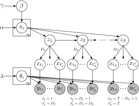
Figure 4: A graphical model for the HDP-HSMM in which the number of segments $S$, and hence the number of nodes, is random.

3.3 Factorial Structure

We can easily compose our sequential models into other common model structures, such as the factorial structure of the factorial HMM (Ghahramani and Jordan, 1997). Factorial models are very useful for source separation problems, and when combined with the rich class of sequential models provided by the HSMM, one can use prior duration information about each source to greatly improve performance (as demonstrated in Section 5). Here, we briefly outline the factorial model and its uses.

If we use $y\sim\text{HDP-HSMM}(\alpha,\gamma,H,G)$ to denote an observation sequence generated by the process defined in Equations 20 to 25, then the generative process for a factorial HDP-HSMM with $K$ component sequences can be written

$$y^{(k)}\sim\text{HDP-HSMM}(\alpha_{k},\gamma_{k},H_{k},G_{k}) k=1,2,\ldots,K$$ (26)

$$\bar{y}_{t}\mathrel{\mathop{\mathchar 58\relax}}=\sum_{k=1}^{K}y_{t}^{(k)}+w_{t} t=1,2,\ldots,T$$ (27)

where $w_{t}$ is a noise process independent of the other components of the model states.

A graphical model for a factorial HMM can be seen in Figure 5, and a factorial HSMM or factorial HDP-HSMM simply replaces the hidden state chains with semi-Markov chains. Each chain, indexed by superscripts, evolves with independent dynamics and produces independent emissions, but the observations are combinations of the independent emissions. Note that each component HSMM is not restricted to any fixed number of states.

Such factorial models are natural ways to frame source separation or disaggregation problems, i.e., identifying component emissions and component states. With the Bayesian framework, we also model uncertainty and ambiguity in such a separation. In Section 5.2 we demonstrate the use of a factorial HDP-HSMM for the task of disaggregating home power signals.

Problems in source separation or disaggregation are often ill-conditioned, and so one relies on prior information in addition to the source independence structure to solve the separation problem. Furthermore, representation of uncertainty is often important, since there may be several good explanations for the data. These considerations motivate Bayesian inference as well as direct modeling of state duration statistics.

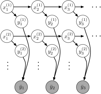
Figure 5: A graphical model for the factorial HMM, which can naturally be extended to factorial structures involving the HSMM or HDP-HSMM.

4 Inference Algorithms

We describe two Gibbs sampling inference algorithms, beginning with a sampling algorithm for the finite Bayesian HSMM, which is built upon in developing algorithms for the HDP-HSMM in the sequel. Next, we develop a weak-limit Gibbs sampling algorithm for the HDP-HSMM, which parallels the popular weak-limit sampler for the HDP-HMM and its sticky extension. Finally, we introduce a collapsed sampler which parallels the direct assignment sampler of (Teh et al., 2006). For all both of the HDP-HSMM samplers there is a loss of conjugacy with the HDP prior due to the fact that self-transitions in the super-state sequence are not permitted (see Section 4.2.1). We develop auxiliary variables to form an augmented representation that effectively recovers conjugacy and hence enables fast exact Gibbs steps.

In comparing the weak limit and direct assignment sampler, the most important trade-offs are that the direct assignment sampler works with the infinite model by integrating out the transition matrix $\pi$ while simplifying bookkeeping by maintaining part of $\beta$; it also collapses the observation and duration parameters. However, the variables in the label sequence $(x_{t})$ are coupled by the integration, and hence each element of the label sequence must be resampled sequentially. In contrast, the weak limit sampler represents all latent components of the model (up to an adjustable finite approximation for the HDP) and thus allows block resampling of the label sequence by exploiting HSMM message passing.

We end the section with a discussion of leveraging changepoint side-information to greatly accelerate inference.

4.1 A Gibbs Sampler for the Finite Bayesian HSMM

4.1.1 Outline of Gibbs Sampler

To perform posterior inference in a finite Bayesian HSMM, we construct a Gibbs sampler resembling that for finite HMMs. Our goal is to construct samples from the posterior

$$p((x_{t}),\{\theta_{i}\},\{\pi_{i}\},\{\omega_{i}\}|(y_{t}),H,G,\alpha)$$ (28)

by drawing samples from the distribution, where $G$ represents the prior over duration parameters. We can construct these samples by following a Gibbs sampling algorithm in which we iteratively sample from the appropriate conditional distributions of $(x_{t})$, $\{\pi_{i}\}$, $\{\omega_{i}\}$, and $\{\theta_{i}\}$.

Sampling $\{\theta_{i}\}$ or $\{\omega_{i}\}$ from their respective conditional distributions can be easily reduced to standard problems depending on the particular priors chosen. Sampling the transition matrix rows $\{\pi_{i}\}$ is straightforward if the prior on each row is Dirichlet over the off-diagonal entries and so we do not discuss it in this section, but we note that when the rows are tied together hierarchically (as in the weak-limit approximation to the HDP-HSMM), resampling the $\{\pi_{i}\}$ correctly requires particular care (see Section 4.2.1).

Sampling $(x_{t})|\{\theta_{i}\},\{\pi_{i}\},(y_{t})$ in a finite Bayesian Hidden semi-Markov Model was first introduced in (Johnson and Willsky, 2010) and, in independent work, later in Dewar et al. (2012). In the following section we develop the algorithm for block-sampling the state sequence $(x_{t})$ from its conditional distribution by employing the HSMM message-passing scheme.

4.1.2 Blocked Conditional Sampling of $(x_{t})$ with Message Passing

To block sample $(x_{t})|\{\theta_{i}\},\{\pi_{i}\},\{\omega_{i}\},(y_{t})$ in an HSMM we can extend the standard block state sampling scheme for an HMM. The key challenge is that to block sample the states in an HSMM we must also be able to sample the posterior duration variables.

If we compute the backwards messages $B$ and $B^{*}$ described in Section 2.2, then we can easily draw a posterior sample for the first state according to:

$$p(x_{1}=k|y_{1\mathrel{\mathop{\mathchar 58\relax}}T}) \propto p(x_{1}=k)p(y_{1\mathrel{\mathop{\mathchar 58\relax}}T}|x_{1}=k,F_{0}=1)$$ (29)

$$=p(x_{1}=k)B^{*}_{0}(k)$$ (30)

where we have used the assumption that the observation sequence begins on a segment boundary ($F_{0}=1$) and suppressed notation for conditioning on parameters.

We can also use the messages to efficiently draw a sample from the posterior duration distribution for the sampled initial state. Conditioning on the initial state draw, $\bar{x}_{1}$, the posterior duration of the first state is:

$$p( D_{1}=d|y_{1\mathrel{\mathop{\mathchar 58\relax}}T},x_{1}=\bar{x}_{1},F_{0}=1)=\frac{p(D_{1}=d,y_{1\mathrel{\mathop{\mathchar 58\relax}}T}|x_{1}=\bar{x}_{1},F_{0})}{p(y_{1\mathrel{\mathop{\mathchar 58\relax}}T}|x_{1}=\bar{x}_{1},F_{0})}$$ (31)

$$=\frac{p(D_{1}=d|x_{1}=\bar{x}_{1},F_{0})p(y_{1\mathrel{\mathop{\mathchar 58\relax}}d}|D_{1}=d,x_{1}=\bar{x}_{1},F_{0})p(y_{d+1\mathrel{\mathop{\mathchar 58\relax}}T}|D_{1}=d,x_{1}=\bar{x}_{1},F_{0})}{p(y_{1\mathrel{\mathop{\mathchar 58\relax}}T}|x_{1}=\bar{x}_{1},F_{0})}$$ (32)

$$=\frac{p(D_{1}=d)p(y_{1\mathrel{\mathop{\mathchar 58\relax}}d}|D_{1}=d,x_{1}=\bar{x}_{1},F_{0}=1)B_{d}(\bar{x}_{1})}{B_{0}^{*}(\bar{x}_{1})}.$$ (33)

We repeat the process by using $x_{D_{1}+1}$ as our new initial state with initial distribution $p(x_{D_{1}+1}=i|x_{1}=\bar{x}_{1})$, and thus draw a block sample for the entire label sequence.

4.2 A Weak-Limit Gibbs Sampler for the HDP-HSMM

The weak-limit sampler for an HDP-HMM (Fox et al., 2008) constructs a finite approximation to the HDP transitions prior with finite $L$-dimensional Dirichlet distributions, motivated by the fact that the infinite limit of such a construction converges in distribution to a true HDP:

$$\beta|\gamma \sim\text{Dir}(\gamma/L,\ldots,\gamma/L)$$ (34)

$$\pi_{i}|\alpha,\beta \sim\text{Dir}(\alpha\beta_{1},\ldots,\alpha\beta_{L}) i=1,\ldots,L$$ (35)

where we again interpret $\pi_{i}$ as the transition distribution for state $i$ and $\beta$ as the distribution which ties state distributions together and encourages shared sparsity. Practically, the weak limit approximation enables the complete representation of the transition matrix in a finite form, and thus, when we also represent all parameters, allows block sampling of the entire label sequence at once, resulting in greatly accelerated mixing in many circumstances. The parameter $L$ gives us control over the approximation, with the guarantee that the approximation will become exact as $L$ grows; see (Ishwaran and Zarepour, 2000), especially Theorem 1, for a discussion of theoretical guarantees. Note that the weak limit approximation is more convenient for us than the truncated stick-breaking approximation because it directly models the state transition probabilities, while stick lengths in the HDP do not directly represent state transition probabilities because multiple sticks in constructing $\pi_{i}$ can be sampled at the same atom of $\beta$.

We can employ the weak limit approximation to create a finite HSMM that approximates inference in the HDP-HSMM. This approximation technique often results in greatly accelerated mixing, and hence it is the technique we employ for the experiments in the sequel. However, the inference algorithm of Section 4.1 must be modified to incorporate the fact that the $\{\pi_{i}\}$ are no longer mutually independent and are instead tied through the shared $\beta$. This dependence between the transition rows introduces potential conjugacy issues with the hierarchical Dirichlet prior; the following section explains the difficulty as well as a clean solution via auxiliary variables.

The beam sampling technique Van Gael et al. (2008) can be applied here with little modification, as in Dewar et al. (2012), to sample over the approximation parameter $L$, thus avoiding the need to set $L$ a priori while still allowing instantiation of the transition matrix and block sampling of the state sequence. This technique is especially useful if the number of states could be very large and is difficult to bound a priori. We do not explore beam sampling here.

4.2.1 Conditional Sampling of $\{\pi_{i}\}$ with Data Augmentation

To construct our overall Gibbs sampler, we need to be able to easily resample the transition matrix $\pi$ given the other components of the model. However, by ruling out self-transitions while maintaining a hierarchical link between the transition rows, the model is no longer fully conjugate, and hence resampling is not necessarily easy. To observe the loss of conjugacy using the hierarchical prior required in the weak-limit approximation, note that we can summarize the relevant portion of the generative model as

$$\beta|\gamma \sim\text{Dir}(\gamma,\ldots,\gamma)$$ (36)

$$\pi_{j}|\beta \sim\text{Dir}(\alpha\beta_{1},\ldots,\alpha\beta_{L}) j=1,\ldots,L$$ (37)

$$x_{t}|\{\pi_{j}\},x_{t-1} \sim\bar{\pi}_{x_{t-1}} t=2,\ldots,T$$ (38)

where $\bar{\pi}_{j}$ represents $\pi_{j}$ with the $j$th component removed and renormalized appropriately:

$$\bar{\pi}_{ji}=\frac{\pi_{ji}(1-\delta_{ij})}{1-\pi_{jj}}$$ (40)

with $\delta_{ij}=1$ if $i=j$ and $\delta_{ij}=0$ otherwise. The deterministic transformation from $\pi_{j}$ to $\bar{\pi}_{j}$ eliminates self-transitions. Note that we have suppressed the observation parameter set, duration parameter set, and observation sequence sampling for simplicity.

Consider the distribution of $\pi_{1}|(x_{t}),\beta$, the first row of the transition matrix:

$$p(\pi_{1}|(x_{t}),\beta) \propto p(\pi_{1}|\beta)p((x_{t})|\pi_{1})$$ (41)

$$\propto\pi_{11}^{\alpha\beta_{1}-1}\pi_{12}^{\alpha\beta_{2}-1}\cdots\pi_{1L}^{\alpha\beta_{L}-1}\left(\frac{\pi_{12}}{1-\pi_{11}}\right)^{n_{12}}\left(\frac{\pi_{13}}{1-\pi_{11}}\right)^{n_{13}}\cdots\left(\frac{\pi_{1L}}{1-\pi_{11}}\right)^{n_{1L}}$$ (42)

where $n_{ij}$ are the number of transitions from state $i$ to state $j$ in the state sequence $(x_{t})$. Essentially, because of the extra $\frac{1}{1-\pi_{11}}$ terms from the likelihood without self-transitions, we cannot reduce this expression to the Dirichlet form over the components of $\pi_{1}$, and therefore we cannot proceed with sampling $m$ and resampling $\beta$ and $\pi$ as in Teh et al. (2006).

However, we can introduce auxiliary variables to recover conjugacy, following the general data augmentation technique described in (Van Dyk and Meng, 2001). We define an extended generative model with extra random variables, and then show through simple manipulations that conditional distributions simplify with the additional variables, hence allowing us to cycle simple Gibbs updates to produce a sampler.

For simplicity, we focus on the first row of the transition matrix, namely $\pi_{1}$, and the draws that depend on it; the reasoning easily extends to the other rows. We also drop the parameter $\alpha$ for convenience. First, we write the relevant portion of the generative process as

$$\pi_{1}|\beta \sim\text{Dir}(\beta)$$ (43)

$$z_{i}|\bar{\pi}_{1} \sim\bar{\pi}_{1}\quad i=1,\ldots,n$$ (44)

$$y_{i}|z_{i} \sim f(z_{i})\quad i=1,\ldots,n$$ (45)

Here, $n$ counts the total number of transitions out of state $1$ and the $\{z_{i}\}$ represent the transitions out of state $1$ to a specific state: sampling $z_{i}=k$ represents a transition from state $1$ to state $k$. The $\{y_{i}\}$ represent the observations on which we condition; in particular, if we have $z_{i}=k$ then the $y_{i}$ corresponds to an emission from state $k$ in the HSMM. See the graphical model in Figure 6 for a depiction of the relationship between the variables.

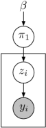
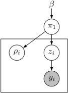
Figure 6: Simplified depiction of the relationship between the auxiliary variables and the rest of the model; 6 depicts the nonconjugate setting and 6 shows the introduced auxiliary variables $\{\rho_{i}\}$.

We can introduce auxiliary variables $\{\rho_{i}\}_{i=1}^{n}$, where each $\rho_{i}$ is independently drawn from a geometric distribution supported on $\{0,1,\ldots\}$ with success parameter $1-\pi_{11}$, i.e. $\rho_{i}|\pi_{11}\sim\text{Geo}(1-\pi_{11})$ (See Figure 6). Thus our posterior becomes:

$$p(\pi_{1}|\{z_{i}\},\{\rho_{i}\}) \propto p(\pi_{1})p(\{z_{i}\}|\pi_{1})p(\{\rho_{i}\}|\{\pi_{1i}\})$$ (46)

$$\propto\pi_{11}^{\beta_{1}-1}\pi_{12}^{\beta_{2}-1}\cdots\pi_{1L}^{\beta_{L}-1}\left(\frac{\pi_{12}}{1-\pi_{11}}\right)^{n_{2}}\cdots\left(\frac{\pi_{1L}}{1-\pi_{11}}\right)^{n_{L}}\left(\prod_{i=1}^{n}\pi_{11}^{\rho_{i}}(1-\pi_{11})\right)$$ (47)

$$=\pi_{11}^{\beta_{1}+\sum_{i}\rho_{i}-1}\pi_{12}^{\beta_{2}+n_{2}-1}\cdots\pi_{1L}^{\beta_{L}+n_{L}-1}$$ (48)

$$\propto\text{Dir}\left(\beta_{1}+\sum_{i}\rho_{i},\beta_{2}+n_{2},\ldots,\beta_{L}+n_{L}\right).$$ (49)

Noting that $n=\sum_{i}n_{i}$, we recover conjugacy and hence can iterate simple Gibbs steps.

We can compare the numerical performance of the auxiliary variable sampler to a Metropolis-Hastings sampler in the simplified model. For a detailed evaluation, see Johnson and Willsky (2012); in deference to space considerations, we only reproduce two figures from that report here. Figure 7 shows the sample chain autocorrelations for the first component of $\pi$ in both samplers. Figure 8 compares the Multivariate Scale Reduction Factors of Brooks and Gelman (1998) for the two samplers, where good mixing is indicated by achieving the statistic’s asymptotic value of unity.

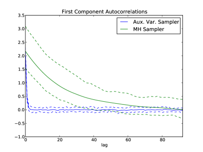
Figure 7: Empirical sample chain autocorrelation for the first component of $\pi$ for both the proposed auxiliary variable sampler and a Metropolis-Hastings sampler. The rapidly diminishing autocorrelation for the auxiliary variable sampler is indicative of fast mixing.

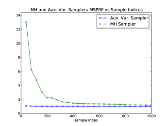
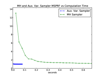
Figure 8: Multivariate Potential Scale Reduction Factors for both the proposed auxiliary variable sampler and a Metropolis-Hastings sampler. The auxiliary variable sampler rapidly achieves the statistic’s asymptotic value of unity. Note that the auxiliary variable sampler is also much more efficient to execute, as shown in 8.

We can easily extend the data augmentation to the full HSMM, and once we have augmented the data with the auxiliary variables $\{\rho_{s}\}$ we are once again in the conjugate setting. A graphical model for the weak-limit approximation to the HDP-HSMM including the auxiliary variables is shown in Figure 9.

For a more detailed derivation as well as further numerical experiments, see Johnson and Willsky (2012).

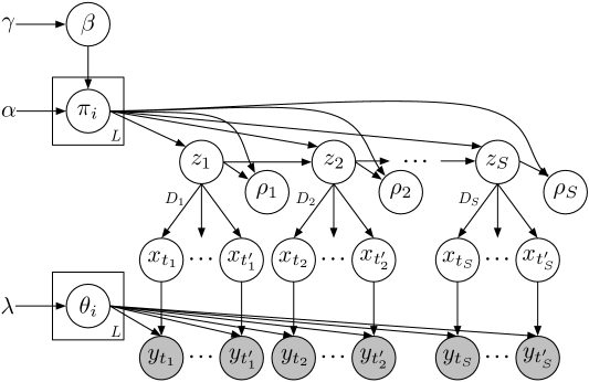
Figure 9: Graphical model for the weak-limit approximation including auxiliary variables.

4.3 A Direct Assignment Sampler for the HDP-HSMM

Though all the experiments in this paper are performed with the weak-limit sampler, we provide a direct assignment (DA) sampler as well for theoretical completeness and because it may be useful in cases where there is insufficient data to inform some latent parameters so that marginalization is necessary for mixing or estimating marginal likelihoods (such as in some topic models). As mentioned previously, in the direct assignment sampler for the HDP-HMM the infinite transition matrix $\pi$ is analytically marginalized out along with the observation parameters (if conjugate priors are used). The sampler represents explicit instantiations of the state sequence $(x_{t})$ and the “used” prefix of the infinite vector $\beta$: $\beta_{1\mathrel{\mathop{\mathchar 58\relax}}K}$ where $K=\#\{x_{t}\mathrel{\mathop{\mathchar 58\relax}}t=1,\ldots,T\}$. There are also auxiliary variables $m$ used to resample $\beta$, but for simplicity we do not discuss them here; see (Teh et al., 2006) for details.

Our DA sampler additionally represents the auxiliary variables necessary to recover HDP conjugacy (as introduced in the previous section). Note that the requirement for, and correctness of, the auxiliary variables described in the finite setting in Section 4.2.1 immediately extends to the infinite setting as a consequence of the Dirichlet Process’s definition in terms of the finite Dirichlet distribution and the Kolmogorov extension theorem (Çinlar, 2010, Ch. 4); for a detailed discussion, see (Orbanz, 2009). The connection to the finite case can also be seen in the sampling steps of the direct assignment sampler for the HDP-HMM, in which the global weights $beta$ over $K$ instantiated components are resampled according to $(\beta_{1\mathrel{\mathop{\mathchar 58\relax}}K},\beta_{\text{rest}})|\alpha\sim\text{Dir}(\alpha+n_{1},\ldots,\alpha+n_{K},\alpha)$ where $n_{i}$ is the number of transitions into state $i$ and Dir is the finite Dirichlet distribution.

4.3.1 Resampling $(x_{t})$

As described in (Fox, 2009), the basic HDP-HMM DA sampling step for each element $x_{t}$ of the label sequence is to sample a new label $k$ with probability proportional (over $k$) to

$$p(x_{t}=k|(x_{\setminus t}),\beta)\propto\underbrace{\frac{\alpha\beta_{k}+n_{x_{t-1},k}}{\alpha+n_{x_{t-1},\cdot}}}_{\text{left-transition}}\cdot\underbrace{\frac{\alpha\beta_{x_{t+1}}+n_{k,x_{t+1}}+\mathbf{1}[x_{t-1}=k=x_{t+1}]}{\alpha+n_{k,\cdot}+\mathbf{1}[x_{t-1}=k]}}_{\text{right-transition}}\cdot\underbrace{f_{\text{obs}}(y_{t}|x_{t}=k)}_{\text{observation}}$$ (50)

for $k=1,\ldots,K+1$ where $K=\#\{x_{t}\mathrel{\mathop{\mathchar 58\relax}}t=1,\ldots,T\}$ and where $\mathbf{1}$ is an indicator function taking value $1$ if its argument condition is true and $0$ otherwise. The variables $n_{ij}$ are transition counts in the portion of the state sequence we are conditioning on, i.e. $n_{ij}=\#\{x_{\tau}=i,x_{\tau+1}=j\mathrel{\mathop{\mathchar 58\relax}}\tau\in\{1,\ldots,T-1\}\setminus\{t-1,t\}\}$. The function $f_{\text{obs}}$ is a predictive likelihood:

$$f_{\text{obs}}( y_{t}|k)\mathrel{\mathop{\mathchar 58\relax}}=p(y_{t}|x_{t}=k,\{y_{\tau}\mathrel{\mathop{\mathchar 58\relax}}x_{\tau}=k\},H)$$ (51)

$$=\int_{\theta_{k}}\underbrace{p(y_{t}|x_{t}=k,\theta_{k})}_{\text{likelihood}}\underbrace{\prod_{\tau\mathrel{\mathop{\mathchar 58\relax}}x_{\tau}=k}p(y_{\tau}|x_{\tau}=k,\theta_{k})}_{\text{likelihood of data with same label}}\underbrace{p(\theta_{k}|H)}_{\text{observation parameter prior}}\;\operatorname{d\!}\theta_{k}$$ (52)

We can derive this step by writing the complete joint probability $p((x_{t}),(y_{t})|\beta,H)$ leveraging exchangeability; this joint probability value is proportional to the desired posterior probability $p(x_{t}|(x_{\setminus t}),(y_{t}),\beta,H)$. When we consider each possible assignment $x_{t}=k$, we can cancel all the terms that are invariant over $k$, namely all the transition probabilities other than those to and from $x_{t}$ and all data likelihoods other than that for $y_{t}$. However, this cancellation process relies on the fact that for the HDP-HMM there is no distinction between self-transitions and new transitions: the term for each $t$ in the complete posterior simply involves transition scores no matter the labels of $x_{t+1}$ and $x_{t-1}$. In the HDP-HSMM case, we must consider segments and their durations separately from transitions.

To derive an expression for resampling $x_{t}$ in the case of the HDP-HSMM, we can similarly consider writing out an expression for the joint probability $p((x_{t}),(y_{t})|\beta,H,G)$, but we notice that as we vary our assignment of $x_{t}$ over $k$, the terms in the expression must change: if $x_{t-1}=\bar{k}$ or $x_{t+1}=\bar{k}$, the probability expression includes a segment term for entire contiguous run of label $\bar{k}$. Hence, since we can only cancel terms that are invariant over $k$, our score expression must include terms for the adjacent segments into which $x_{t}$ may merge. See Figure 10 for an illustration.

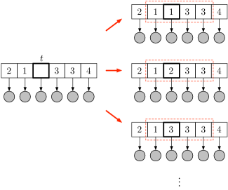
Figure 10: Illustration of the Gibbs step to resample $x_{t}$ for the DA sampler for the HDP-HSMM. The red boxes indicate the elements of the label sequence that contribute to the score computation for $k=1,2,3$ which produce two, three, and two segment terms, respectively. The label sequence element being resample is emphasized in bold.

The final expression for the probability of sampling the new value of $x_{t}$ to be $k$ then consists of between 1 and 3 segment score terms, depending on merges with adjacent segments, each of which has the form

$$p(x_{t}=k|(x_{\setminus t}),\beta,H,G)\propto\underbrace{\frac{\alpha\beta_{k}+n_{x_{\text{prev}},k}}{\alpha(1-\beta_{x_{\text{prev}}})+n_{x_{\text{prev}},\cdot}}}_{\text{left-transition}}\cdot\underbrace{\frac{\alpha\beta_{x_{\text{next}}}+n_{k,x_{\text{next}}}}{\alpha(1-\beta_{k})+n_{k,\cdot}}}_{\text{right-transition}}$$ (53)

$$\cdot\underbrace{f_{\text{dur}}(t^{2}-t^{1}+1)}_{\text{duration}}\cdot\underbrace{f_{\text{obs}}(y_{t^{1}\mathrel{\mathop{\mathchar 58\relax}}t^{2}}|k)}_{\text{observation}}$$ (54)

where we have used $t^{1}$ and $t^{2}$ to denote the first and last indices of the segment, respectively. Transition scores at the start and end of the chain are not included.

The function $f_{\text{dur}}(d|k)$ is the corresponding duration predictive likelihood evaluated on a duration $d$, which depends on the durations of other segments with label $k$ and any duration hyperparameters. The function $f_{\text{obs}}$ now represents a block or joint predictive likelihood over all the data in a segment (see e.g. (Murphy, 2007) for a thorough discussion of the Gaussian case). Note that the denominators in the transition terms are affected by the elimination of self-transitions by a rescaling of the “total mass.” The resulting chain is ergodic if the duration predictive score $f_{\text{dur}}$ has a support that includes $\{1,2,\ldots,d_{\text{max}}\}$, so that segments can be split and merged in any combination.

4.3.2 Resampling $\beta$ and Auxiliary Variables $\rho$

To allow conjugate resampling of $\beta$, auxiliary variables must be introduced to deal with the conjugacy issue raised in Section 4.2. In the direct assignment samplers, the auxiliary variables are not used to resample diagonal entries of the transition matrix $\pi$, which is marginalized out, but rather to directly resample $\beta$. In particular, with each segment $s$ we associate an auxiliary count $\rho_{s}$ which is independent of the data and only serves to preserve conjugacy in the HDP. We periodically re-sample via

$$\pi_{ii}|\alpha,\beta \sim\text{Beta}(\alpha\beta_{i},\alpha(1-\beta_{i}))$$ (55)

$$\rho_{s}|\pi_{ii},z_{s} \sim\text{Geo}(1-\pi_{z_{s},z_{s}})$$ (56)

The count $n_{i,i}$, which is used in resampling the auxiliary variables $m$ of Teh et al. (2006) which in turn are then used to resample $\beta$, is the total of the auxiliary variables for other segments with the same label, i.e. $n_{i,i}=\sum_{\bar{s}\neq s,z_{\bar{s}}=z_{s}}\rho_{\bar{s}}$. This formula can be interpreted as simply sampling the number of self-transitions we may have seen at segment $s$ given $\beta$ and the counts of self- and non-self transitions in the super-state sequence. Note $\pi_{ii}$ is independent of the data given $(z_{s})$; as before, this auxiliary variable procedure is a convenient way to integrate out numerically the diagonal entries of the transition matrix.

By using the total auxiliary as the statistics for $n_{i,i}$, we can resample $\beta|(x_{t}),\alpha,\gamma$ according to the procedure for the HDP-HMM as described in (Teh et al., 2006).

4.4 Exploiting Changepoint Side-Information

In many circumstances, we may not need to consider all time indices as possible changepoints at which the super-state may switch; it may be easy to rule out many non-changepoints from consideration. For example, in the power disaggregation application in Section 5, we can run inexpensive changepoint detection on the observations to get a list of possible changepoints, ruling out many obvious non-changepoints. The possible changepoints divide the label sequence into state blocks, where within each block the label sequence must be constant, though sequential blocks may have the same label. By only allowing super-state switching to occur at these detected changepoints, we can greatly reduce the computation of all the samplers considered.

In the case of the weak-limit sampler, the complexity of the bottleneck message-passing step is reduced to a function of the number of possible changepoints (instead of total sequence length): the asymptotic complexity becomes $\mathcal{O}(T_{\text{change}}^{2}N+N^{2}T_{\text{change}})$ , where $T_{\text{change}}$, the number of possible changepoints, may be dramatically smaller than the sequence length $T$. We simply modify the backwards message-passing procedure to sum only over the possible durations:

$$B_{t}^{*}(i) \mathrel{\mathop{\mathchar 58\relax}}=p(y_{t+1\mathrel{\mathop{\mathchar 58\relax}}T}|x_{t+1}=i,F_{t}=1)$$ (57)

$$=\sum_{d\in\mathbb{D}}B_{t+d}(i)\underbrace{\tilde{p}(D_{t+1}=d|x_{t+1}=i)}_{\text{duration prior term}}\cdot\underbrace{p(y_{t+1\mathrel{\mathop{\mathchar 58\relax}}t+d}|x_{t+1}=i,D_{t+1}=d)}_{\text{likelihood term}}$$ (58)

$$\quad+\underbrace{\tilde{p}(D_{t+1}>T-t|x_{t+1}=i)p(y_{t+1\mathrel{\mathop{\mathchar 58\relax}}T}|x_{t+1}=i,D_{t+1}>T-t)}_{\text{censoring term}}$$ (59)

where $\tilde{p}$ represents the duration distribution restricted to the set of possible durations $\mathbb{D}\subset\mathbb{N}^{+}$ and re-normalized. We similarly modify the forward-sampling procedure to only consider possible durations. It is also clear how to adapt the DA sampler: instead of re-sampling each element of the label sequence $(x_{t})$ we simply consider the block label sequence, resampling each block’s label (allowing merging with adjacent blocks).

5 Experiments

In this section, we evaluate the proposed HDP-HSMM sampling algorithms on both synthetic and real data. First, we compare the HDP-HSMM direct assignment sampler to the weak limit sampler as well as the Sticky HDP-HMM direct assignment sampler, showing that the HDP-HSMM direct assignment sampler has similar performance to that for the Sticky HDP-HMM and that the weak limit sampler is much faster. Next, we evaluate the HDP-HSMM weak limit sampler on synthetic data generated from finite HSMMs and HMMs. We show that the HDP-HSMM applied to HSMM data can efficiently learn the correct model, including the correct number of states and state labels, while the HDP-HMM is unable to capture non-geometric duration statistics. We also apply the HDP-HSMM to data generated by an HMM and demonstrate that, when equipped with a duration distribution class that includes geometric durations, the HDP-HSMM can also efficiently learn an HMM model when appropriate with little loss in efficiency. Next, we use the HDP-HSMM in a factorial (Ghahramani and Jordan, 1997) structure for the purpose of disaggregating a whole-home power signal into the power draws of individual devices. We show that encoding simple duration prior information when modeling individual devices can greatly improve performance, and further that a Bayesian treatment of the parameters is advantageous. We also demonstrate how changepoint side-information can be leveraged to significantly speed up computation. The Python code used to perform these experiments as well as Matlab code is available online at http://github.com/mattjj/pyhsmm.

5.1 Synthetic Data

Figure 11 compares the HDP-HSMM direct assignment sampler to that of the Sticky HDP-HMM as well as the HDP-HSMM weak limit sampler. Figure 11 shows that the direct assignment sampler for a Geometric-HDP-HSMM performs similarly to the Sticky HDP-HSMM direct assignment sampler when applied to data generated by an HMM with scalar Gaussian emissions. Figures 11 shows that the weak limit sampler mixes much more quickly than the direct assignment sampler. Each iteration of the weak limit sampler is also much faster to execute (approximately 50x faster in our implementations in Python). Due to its much greater efficiency, we focus on the weak limit sampler for the rest of this section; we believe it is a superior inference algorithm whenever an adequately large approximation parameter $L$ can be chosen a priori.

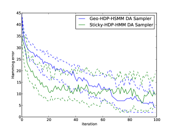
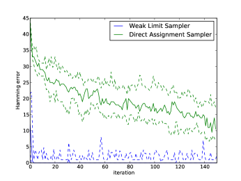
Figure 11: 11 compares the Geometric-HDP-HSMM direct assignment sampler with that of the Sticky HDP-HMM, both applied to HMM data. The sticky parameter $\kappa$ was chosen to maximize mixing. 11 compares the HDP-HSMM direct assignment sampler with the weak limit sampler. In all plots, solid lines are the median error at each time over 25 independent chains; dashed lines are 25th and 75th percentile errors.

Figure 12 summarizes the results of applying both a Poisson-HDP-HSMM and an HDP-HMM to data generated from an HSMM with four states, Poisson durations, and 2-dimensional mixture-of-Gaussian emissions. In the 25 Gibbs sampling runs for each model, we applied 5 chains to each of 5 generated observation sequences. The HDP-HMM is unable to capture the non-Markovian duration statistics and so its state sampling error remains high, while the HDP-HSMM equipped with Poisson duration distributions is able to effectively learn the correct temporal model, including duration, transition, and emission parameters, and thus effectively separate the states and significantly reduce posterior uncertainty. The HDP-HMM also frequently fails to identify the true number of states, while the posterior samples for the HDP-HSMM concentrate on the true number; see Figure 13.

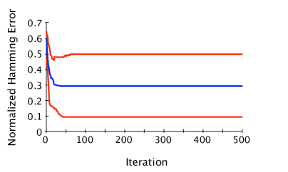
(a) HDP-HMM

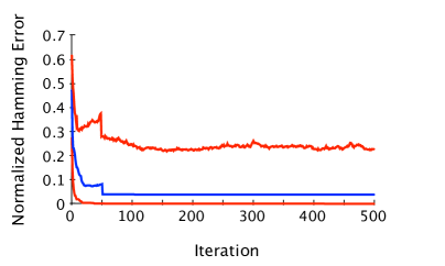
(b) HDP-HSMM

Figure 12: State-sequence Hamming error of the HDP-HMM and Poisson-HDP-HSMM applied to data from a Poisson-HSMM. In each plot, the blue line indicates the error of the chain with the median error across 25 independent Gibbs chains, while the red lines indicate the chains with the 10th and 90th percentile errors at each iteration. The jumps in the plot correspond to a change in the ranking of the 25 chains.

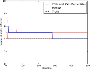
(a) HDP-HSMM

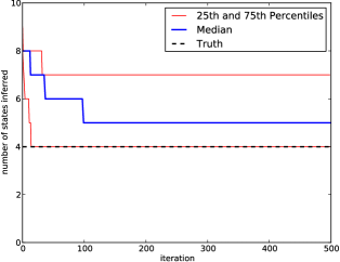
(b) HDP-HMM

Figure 13: Number of states inferred by the HDP-HMM and Poisson-HDP-HSMM applied to data from a four-state Poisson-HSMM. In each plot, the blue line indicates the error of the chain with the median error across 25 independent Gibbs chains, while the red lines indicate the chains with the 10th and 90th percentile errors at each iteration.

By setting the class of duration distributions to be a superclass of the class of geometric distributions, we can allow an HDP-HSMM model to learn an HMM from data when appropriate. One such distribution class is the class of negative binomial distributions, denoted $\text{NegBin}(r,p)$, the discrete analog of the Gamma distribution, which covers the class of geometric distributions when $r=1$. By placing a (non-conjugate) prior over $r$ that includes $r=1$ in its support, we allow the model to learn geometric durations as well as significantly non-geometric distributions with modes away from zero. Figure 14 shows a negative binomial HDP-HSMM learning an HMM model from data generated from an HMM with four states. The observation distribution for each state is a 10-dimensional Gaussian, again with parameters sampled i.i.d. from a NIW prior. The prior over $r$ was set to be uniform on $\{1,2,\ldots,6\}$, and all other priors were chosen to be similarly non-informative. The sampler chains quickly concentrated at $r=1$ for all state duration distributions. There is only a slight loss in mixing time for the HDP-HSMM compared to the HDP-HMM. This experiment demonstrates that with the appropriate choice of duration distribution the HDP-HSMM can effectively learn an HMM model.

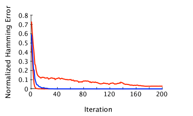
(a) HDP-HMM

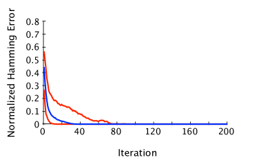
(b) HDP-HSMM

Figure 14: The HDP-HSMM and HDP-HMM applied to data from an HMM. In each plot, the blue line indicates the error of the chain with the median error across 25 independent Gibbs chains, while the red line indicates the chains with the 10th and 90th percentile error at each iteration.

5.2 Power Disaggregation

In this section we show an application of the HDP-HSMM factorial structure to an unsupervised power signal disaggregation problem. The task is to estimate the power draw from individual devices, such as refrigerators and microwaves, given an aggregated whole-home power consumption signal. This disaggregation problem is important for energy efficiency: providing consumers with detailed power use information at the device level has been shown to improve efficiency significantly, and by solving the disaggregation problem one can provide that feedback without instrumenting every individual device with monitoring equipment. This application demonstrates the utility of including duration information in priors as well as the significant speedup achieved with changepoint-based inference.

The power disaggregation problem has a rich history (Zeifman and Roth, 2011) with many proposed approaches for a variety of problem specifications. Some recent work (Kim et al., 2010) has considered applying factorial HSMMs to the disaggregation problem using an EM algorithm; our work here is distinct in that (1) we do not use training data to learn device models but instead rely on simple prior information and learn the model details during inference, (2) our states are not restricted to binary values and can model multiple different power modes per device, and (3) we use Gibbs sampling to learn all levels of the model. The work in (Kim et al., 2010) also explores many other aspects of the problem, such as additional data features, and builds a very compelling complete solution to the disaggregation problem, while we focus on the factorial time series modeling itself.

For our experiments, we used the REDD dataset (Kolter and Johnson, 2011), which monitors many homes at high frequency and for extended periods of time. We chose the top 5 power-drawing devices (refrigerator, lighting, dishwasher, microwave, furnace) across several houses and identified 18 24-hour segments across 4 houses for which many (but not always all) of the devices switched on at least once. We applied a 20-second median filter to the data, and each sequence is approximately 5000 samples long.

We constructed simple priors that set the rough power draw levels and duration statistics of the modes for several devices. For example, the power draw from home lighting changes infrequently and can have many different levels, so an HDP-HSMM with a bias towards longer negative-binomial durations is appropriate. On the other hand, a refrigerator’s power draw cycle is very regular and usually exhibits only three modes, so our priors biased the refrigerator HDP-HSMM to have fewer modes and set the power levels accordingly. For details on our prior specification, see Appendix A. We did not truncate the duration distributions during inference, and we set the weak limit approximation parameter $L$ to be twice the number of expected modes for each device; e.g., for the refrigerator device we set $L=6$ and for lighting we set $L=20$. We performed sampling inference independently on each observation sequence.

As a baseline for comparison, we also constructed a factorial sticky HDP-HMM (Fox et al., 2008) with the same observation priors and with duration biases that induced the same average mode durations as the corresponding HDP-HSMM priors. We also compare to the factorial HMM performance presented in (Kolter and Johnson, 2011), which fit device models using an EM algorithm on training data. For the Bayesian models, we performed inference separately on each aggregate data signal.

The set of possible changepoints is easily identifiable in these data, and a primary task of the model is to organize the jumps observed in the observations into an explanation in terms of the individual device models. By simply computing first differences and thresholding, we are able to reduce the number of potential changepoints we need to consider from 5000 to 100-200, and hence we are able to speed up state sequence resampling by orders of magnitude. See Figure 15 for an illustration.

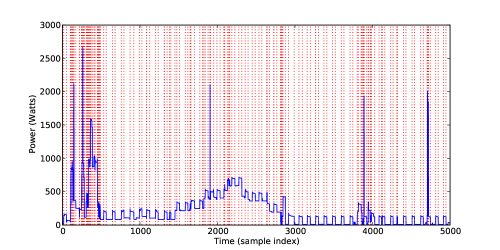
Figure 15: An total power observation sequence from the power disaggregation dataset. Vertical dotted red lines indicate changepoints detected with a simple first-differences. By using the changepoint-based algorithms described in Section 4.4 we can greatly accelerate inference speed for this application.

To measure performance, we used the error metric of (Kolter and Johnson, 2011):

$$\text{Acc.}=1-\frac{\sum_{t=1}^{T}\sum_{i=1}^{K}\left|\hat{y}_{t}^{(i)}-y_{t}^{(i)}\right|}{2\sum_{t=1}^{T}\bar{y}_{t}}$$

where $\bar{y}_{t}$ refers to the observed total power consumption at time $t$, $y^{(i)}_{t}$ is the true power consumed at time $t$ by device $i$, and $\hat{y}_{t}^{(i)}$ is the estimated power consumption. We produced 20 posterior samples for each model and report the median accuracy of the component emission means compared to the ground truth provided in REDD. We ran our experiments on standard desktop machines (Intel Core i7-920 CPUs, released Q4 2008), and a sequence with about 200 detected changepoints would resample each component chain in 0.1 seconds, including block sampling the state sequence and resampling all observation, duration, and transition parameters. We collected samples after every 50 such iterations.

Our overall results are summarized in Figure 16 and Table 1. Both Bayesian approaches improved upon the EM-based approach because they allowed flexibility in the device models that could be fit during inference, while the EM-based approach fixed device model parameters that may not be consistent across homes. Furthermore, the incorporation of duration structure and prior information provided a significant performance increase for the HDP-HSMM approach. Detailed performance comparisons between the HDP-HMM and HDP-HSMM approaches can be seen in Figure 17. Finally, Figures 18 and 19 shows total power consumption estimates for the two models on two selected data sequences.

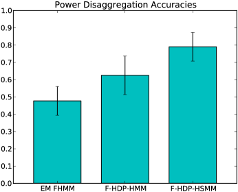
Figure 16: Overall accuracy comparison between the EM-trained FHMM of (Kolter and Johnson, 2011), the factorial sticky HDP-HMM, and the factorial HDP-HSMM.

House	EM FHMM	F-HDP-HMM	F-HDP-HSMM
1	46.6%	69.0%	82.1%
2	50.8%	70.7%	84.8%
3	33.3%	67.3%	81.5%
6	55.7%	61.8%	77.7%
Mean	47.7%	67.2%	81.5%

Table 1: Performance comparison broken down by house.

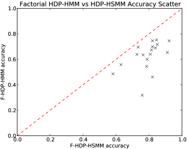
Figure 17: Performance comparison between the HDP-HMM and HDP-HSMM approaches broken down by data sequence.

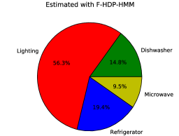
(a) 1

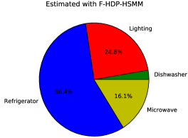
(b) 2

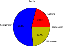
(c) 3

Figure 18: Estimated total power consumption for a data sequence where the HDP-HSMM significantly outperformed the HDP-HMM due to its modeling of duration regularities.

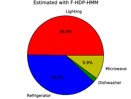
(a) 1

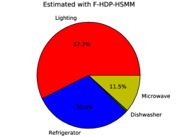
(b) 2

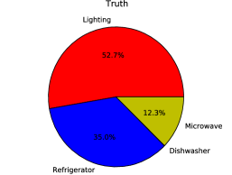
(c) 3

Figure 19: Estimated total power consumption for a data sequence where both the HDP-HMM and HDP-HSMM approaches performed well.

We note that the nonparametric prior was very important for modeling the power consumption due to lighting. Power modes arise from combinations of lights switched on in the user’s home, and hence the number of levels that are observed is highly uncertain a priori. For the other devices the number of power modes (and hence states) is not so uncertain, but duration statistics can provide a strong clue for disaggregation; for these, the main advantage of our model is in providing Bayesian inference and duration modeling.

6 Conclusion

We have developed the HDP-HSMM and two Gibbs sampling inference algorithms, the weak limit and direct assignment samplers, uniting explicit-duration semi-Markov modeling with new Bayesian nonparametric techniques. These models and algorithms not only allow learning from complex sequential data with non-Markov duration statistics in supervised and unsupervised settings, but also can be used as tools in constructing and performing infernece in larger hierarchical models. We have demonstrated the utility of the HDP-HSMM and the effectiveness of our inference algorithms with real and synthetic experiments, and we believe these methods can be built upon to provide new tools for many sequential learning problems.

Acknowledgments

The authors thank J. Zico Kolter, Emily Fox, and Ruslan Salakhutdinov for invaluable discussions and advice. We also thank the anonymous reviewers for helpful fixes and suggestions. This work was supported in part by a MURI through ARO Grant W911NF-06-1-0076, in part through a MURI through AFOSR Grant FA9550-06-1-303, and in part by the National Science Foundation Graduate Research Fellowship under Grant No. 1122374.

A Power Disaggregation Priors

We used simple hand-set priors for the power disaggregation experiments in Section 5.2, where each prior had two free parameters that were set to encode rough means and variances for each device mode’s durations and emissions. To put priors on multiple modes we used atomic mixture models in the priors. For example, refrigerators tend to exhibit an “off” mode near zero Watts, an “on” mode near 100-140 Watts, and a “high” mode near 300-400 Watts; we include each of these regimes in the prior by specifying three sets of hyperparameters, and a state samples observation parameters by first sampling one of the three sets of hyperparameters uniformly at random and then sampling observation parameters using those hyperparameters

A comprehensive summary of our prior settings for the Factorial HDP-HSMM are in Table 2. Observation distributions were all Gaussian with state-specific latent means and fixed variances. We use $\text{Gauss}(\mu_{0},\sigma_{0}^{2};\sigma^{2})$ to denote a Gaussian observation distribution prior with a fixed variance of $\sigma^{2}$ and a prior over its mean parameter that is Gaussian distributed with mean $\mu_{0}$ and variance $\sigma_{0}^{2}$; i.e., it denotes that a state’s mean parameter $\mu$ is sampled according to $\mu\sim\mathcal{N}(\mu_{0},\sigma_{0}^{2})$ and an observation from that state is sampled from $\mathcal{N}(\mu,\sigma^{2})$. Similarly, we use $\text{NegBin}(\alpha,\beta;r)$ to denote Negative Binomial duration distribution priors where a latent state-specific “success” parameter $p$ is drawn from $p\sim\text{Beta}(\alpha,\beta)$ and the parameter $r$ is fixed, so that state durations for that state are then drawn from $\text{NegBin}(p,r)$. (Note choosing $r=1$ sets a geometric duration class.)

We set the priors for the Factorial Sticky HDP-HMM by using the same set of observation prior parameters as for the HDP-HSMM and setting state-specific sticky bias parameters so as to match the expected durations encoded in the HDP-HSMM duration priors. For an example of real data observation sequences, see Figure 20.

A natural extension of this model would be a more elaborate hierarchical model which learns the hyperparameter mixtures automatically from training data. As our experiment is meant to emphasize the merits of the HDP-HSMM and sampling inference, we leave this extension to future work.

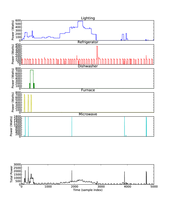
Figure 20: Example real data observation sequences for the power disaggregation experiments.

Device	Base Measures		Specific States
	Observations	Durations	Observations	Durations
Lighting	$\text{Gauss}(300,200^{2};5^{2})$	$\text{NegBin}(5,220;12)$	$\text{Gauss}(0,1;5^{2})$	$\text{NegBin}(5,220;12)$
Refrigerator	$\text{Gauss}(110,50^{2};10^{2})$	$\text{NegBin}(100,600;10)$	$\text{Gauss}(0,1;5^{2})$	$\text{NegBin}(100,600;10)$
			$\text{Gauss}(115,10^{2};10^{2})$	$\text{NegBin}(100,600;10)$
			$\text{Gauss}(425,30^{2};10^{2})$	$\text{NegBin}(100,600;10)$
Dishwasher	$\text{Gauss}(225,25^{2};10^{2})$	$\text{NegBin}(100,200;10)$	$\text{Gauss}(0,1;5^{2})$	$\text{NegBin}(1,2000;1)$
			$\text{Gauss}(225,25^{2};10^{2})$	$\text{NegBin}(100,200;10)$
			$\text{Gauss}(900,200^{2};10^{2})$	$\text{NegBin}(40,500;10)$
Furnace	$\text{Gauss}(600,100^{2};20^{2})$	$\text{NegBin}(40,40;10)$	$\text{Gauss}(0,1;5^{2})$	$\text{NegBin}(1,50;1)$
Microwave	$\text{Gauss}(1700,200^{2};50^{2})$	$\text{NegBin}(200,1;50)$	$\text{Gauss}(0,1;5^{2})$	$\text{NegBin}(1,1000;1)$

Table 2: Power disaggregation prior parameters for each device. Observation priors encode rough power levels that are expected from devices. Duration priors encode duration statistics that are expected from devices.

References

- Beal et al. (2002) M.J. Beal, Z. Ghahramani, and C.E. Rasmussen. The infinite hidden markov model. Advances in neural information processing systems, 14:577–584, 2002.
- Brooks and Gelman (1998) S.P. Brooks and A. Gelman. General methods for monitoring convergence of iterative simulations. Journal of Computational and Graphical Statistics, pages 434–455, 1998.
- Çinlar (2010) E. Çinlar. Probability and Stochastics. Springer Verlag, 2010.
- Dewar et al. (2012) M. Dewar, C. Wiggins, and F. Wood. Inference in hidden markov models with explicit state duration distributions. Signal Processing Letters, IEEE, (99):1–1, 2012.
- Fox et al. (2008) E. B. Fox, E. B. Sudderth, M. I. Jordan, and A. S. Willsky. An HDP-HMM for systems with state persistence. In Proc. International Conference on Machine Learning, July 2008.
- Fox (2009) E.B. Fox. Bayesian Nonparametric Learning of Complex Dynamical Phenomena. Ph.D. thesis, MIT, Cambridge, MA, 2009.
- Ghahramani and Jordan (1997) Z. Ghahramani and M.I. Jordan. Factorial hidden markov models. Machine learning, 29(2):245–273, 1997.
- Guédon (2007) Yann Guédon. Exploring the state sequence space for hidden markov and semi-markov chains. Comput. Stat. Data Anal., 51(5):2379–2409, 2007. ISSN 0167-9473. doi: http://dx.doi.org/10.1016/j.csda.2006.03.015.
- Hashimoto et al. (2009) K. Hashimoto, Y. Nankaku, and K. Tokuda. A bayesian approach to hidden semi-markov model based speech synthesis. In Tenth Annual Conference of the International Speech Communication Association, 2009.
- Heller et al. (2009) K. A. Heller, Y. W. Teh, and D. Görür. Infinite hierarchical hidden Markov models. In Proceedings of the International Conference on Artificial Intelligence and Statistics, volume 12, 2009.
- Ishwaran and Zarepour (2000) H. Ishwaran and M. Zarepour. Markov chain monte carlo in approximate dirichlet and beta two-parameter process hierarchical models. Biometrika, 87(2):371–390, 2000.
- Johnson and Willsky (2010) Matthew J. Johnson and Alan S. Willsky. The Hierarchical Dirichlet Process Hidden Semi-Markov Model. In UAI’10: Proceedings of the Twenty-Sixth Conference on Uncertainty in Artificial Intelligence, Corvallis, Oregon, USA, 2010. AUAI Press.
- Johnson and Willsky (2012) Matthew J. Johnson and Alan S. Willsky. 2012. arXiv:1208.6537v2.
- Kim et al. (2010) H. Kim, M. Marwah, M. Arlitt, G. Lyon, and J. Han. Unsupervised disaggregation of low frequency power measurements. Technical report, HP Labs Tech. Report, 2010.
- Kolter and Johnson (2011) J.Z. Kolter and M.J. Johnson. Redd: A public data set for energy disaggregation research. 2011.
- Murphy (2002) Kevin Murphy. Hidden semi-markov models (segment models). Technical Report, November 2002. URL http://www.cs.ubc.ca/~murphyk/Papers/segment.pdf.
- Murphy (2007) Kevin P. Murphy. Conjugate bayesian analysis of the gaussian distribution. Technical report, 2007.
- Orbanz (2009) P. Orbanz. Construction of nonparametric bayesian models from parametric bayes equations. Advances in neural information processing systems, 2009.
- Sethuraman. (1994) J. Sethuraman. A constructive definition of dirichlet priors. In Statistica Sinica, volume 4, pages 639–650, 1994.
- Teh et al. (2006) Y. W. Teh, M. I. Jordan, M. J. Beal, and D. M. Blei. Hierarchical Dirichlet processes. Journal of the American Statistical Association, 101(476):1566–1581, 2006.
- Tranter and Reynolds (2006) S.E. Tranter and D.A. Reynolds. An overview of automatic speaker diarization systems. Audio, Speech, and Language Processing, IEEE Transactions on, 14(5):1557–1565, 2006.
- Van Dyk and Meng (2001) D.A. Van Dyk and X.L. Meng. The art of data augmentation. Journal of Computational and Graphical Statistics, 10(1):1–50, 2001.
- Van Gael et al. (2008) J. Van Gael, Y. Saatci, Y.W. Teh, and Z. Ghahramani. Beam sampling for the infinite hidden markov model. In Proceedings of the 25th international conference on Machine learning, pages 1088–1095. ACM, 2008.
- Yu (2010) S.Z. Yu. Hidden semi-markov models. Artificial Intelligence, 174(2):215–243, 2010.
- Zeifman and Roth (2011) M. Zeifman and K. Roth. Nonintrusive appliance load monitoring: Review and outlook. Consumer Electronics, IEEE Transactions on, 57(1):76–84, 2011.