The fractional chromatic number
of triangle-free subcubic graphs

Abstract

Heckman and Thomas conjectured that the fractional chromatic number of any triangle-free subcubic graph is at most $14/5$. Improving on estimates of Hatami and Zhu and of Lu and Peng, we prove that the fractional chromatic number of any triangle-free subcubic graph is at most $32/11\approx 2.909$.

1 Introduction

When considering the chromatic number of certain graphs, one may notice colourings which are best possible (in that they use as few colours as possible) but which are in some sense wasteful. For instance, an odd cycle cannot be properly coloured with two colours but can be coloured using three colours in such a way that the third colour is used only once.

Indeed if $C_{7}$ has vertices $v_{1},v_{2},v_{3},\dots,v_{7}$, then we can colour $v_{1},v_{3},v_{5}$ red, $v_{2},v_{4},v_{6}$ blue and $v_{7}$ green. If, however, our aim is instead to assign multiple colours to each vertex such that adjacent vertices receive disjoint lists of colours, then we could double-colour $C_{7}$ using five (rather than six) colours and triple-colour it using seven (rather than nine) colours in such a way that each colour is used exactly three times — colour $v_{i}$ with colours $3i,3i+1,3i+2$ (mod $7$). Asking for the minimum of the ratio of colours required to the number of colours assigned to each vertex gives us a generalisation of the chromatic number.

Alternatively, for a graph $G=(V,E)$ we can consider a function $w$ assigning to each independent set of vertices $I$ a real number $w(I)\in[0,1]$. We call such a function a weighting. The weight $w[v]$ of a vertex $v\in V$ with respect to $w$ is then defined to be the sum of $w(I)$ over all independent sets containing $v$. A weighting $w$ is a fractional colouring of $G$ if for each $v\in V$ $w[v]\geq 1$. The size $|w|$ of a fractional colouring is the sum of $w(I)$ over all independent sets $I$. The fractional chromatic number $\chi_{f}(G)$ is then defined to be the infimum of $|w|$ over all possible fractional colourings. We refer the reader to [bib:SU-fractional] for more information on fractional colourings and the related theory.

By a folklore result, the above two definitions of the fractional chromatic number are equivalent to each other and to a third, probabilistic, definition. It is this third definition which we will make most use of:

Lemma 1.

Let $G$ be a graph and $k$ a positive rational number. The following are equivalent:

1. $\chi_{f}(G)\leq k$,

2. there exists an integer $N$ and a multi-set $\cal W$ of $kN$ independent sets in $G$ such that each vertex is contained in exactly $N$ sets of $\cal W$,

3. there exists a probability distribution $\pi$ on the independent sets of $G$ such that for each vertex $v$, the probability that $v$ is contained in a random independent set (with respect to $\pi$) is at least $1/k$.

In this paper, we consider the problem of bounding the fractional chromatic number of a graph that has maximum degree at most three (we call such graphs subcubic) and contains no triangle. Brooks’ theorem (see, e.g., [bib:Die-graph, Theorem 5.2.4]) asserts that such graphs have chromatic number at most three, and, thus, also have fractional chromatic number at most three. On the other hand, Fajtlowicz [bib:Faj-size] observed that the independence number of the generalised Petersen Graph $P(7,2)$ (Figure 1) equals 5, which implies that $\chi_{f}(P(7,2))=14/5=2.8$.

Figure 1: The generalised Petersen graph.

In 2001, Heckman and Thomas [bib:HT-new] made the following conjecture:

Conjecture 2.

The fractional chromatic number of any triangle-free subcubic graph $G$ is at most $2.8$.

Conjecture 2 is based on the result of Staton [bib:Sta-some] (see also [bib:Jon-size, bib:HT-new]) that any triangle-free subcubic graph contains an independent set of size at least $5n/14$, where $n$ is the number of vertices of $G$. As shown by the graph $P(7,2)$, this result is optimal.

Hatami and Zhu [bib:HZ-fractional] proved that under the same assumptions, $\chi_{f}(G)\leq 3-3/64\approx 2.953$. More recently, Lu and Peng [bib:LP-fractional] were able to improve this bound to $\chi_{f}(G)\leq 3-3/43\approx 2.930$. We offer a new probabilistic proof which improves this bound as follows:

Theorem 3.

The fractional chromatic number of any triangle-free subcubic graph is at most $32/11\approx 2.909$.

We remark that while this paper was under review, Dvořák, Sereni and Volec [bib:DSV-subcubic] succeeded in proving Conjecture 2. Their result was preceded by an improvement of the bound in Theorem 3 to $43/15\approx 2.867$ due to Liu [bib:Liu-upper].

In the rest of this section, we review the necessary terminology. The length of a path $P$, denoted by $\left|{P}\right|$, is the number of its edges. We use the following notation for paths. If $P$ is a path and $x,y\in V(P)$, then $xPy$ is the subpath of $P$ between $x$ and $y$. The same notation is used when $P$ is a cycle with a specified orientation, in which case $xPy$ is the subpath of $P$ between $x$ and $y$ which follows $x$ with respect to the orientation. In both cases, we write $d_{P}(x,y)$ for $\left|{xPy}\right|$.

We distinguish between edges in undirected graphs and arcs in directed graphs. If $xy$ is an arc, then $x$ is its tail and $y$ its head.

If $G$ is a graph and $X,Y\subseteq V(G)$, then $E(X,Y)$ is the set of edges of $G$ with one endvertex in $X$ and the other one in $Y$. We let $\partial(X)$ denote the set $E(X,V(G)-X)$. For a subgraph $H\subseteq G$, we write $\partial(H)$ for $\partial(V(H))$, and we extend the definition of the symbol $E(X,Y)$ to subgraphs in an analogous way. The neighbourhood of a vertex $u$ of $G$ is the set $N(u)$ of its neighbours. We define $N[u]=N(u)\cup\left\{{u}\right\}$ and call this set the closed neighbourhood of $u$.

2 An algorithm

Let $G$ be a simple cubic bridgeless graph. By a well-known theorem of Petersen (see, e.g., [bib:Die-graph, Corollary 2.2.2]), $G$ has a 2-factor. It will be helpful in our proof to pick a 2-factor with special properties, namely one satisfying the condition in the following result of Kaiser and Škrekovski [bib:KS-cycles, Corollary 4.5]:

Theorem 4 ([bib:KS-cycles]).

Every cubic bridgeless graph contains a 2-factor whose edge set intersects each inclusionwise minimal edge-cut in $G$ of size 3 or 4.

Among all 2-factors of $G$ satisfying the condition of Theorem 4, choose a 2-factor $F$ with as many components as possible. The following lemma will be used to rule out some of the cases in the analysis found in Section LABEL:sec:chord:

Lemma 5.

Let $C$ be a cycle of $F$. If there exist vertex-disjoint cycles $D_{1}$ and $D_{2}$ such that $V(C)=V(D_{1})\cup V(D_{2})$, then the following hold:

1. $2\leq\left|{E(D_{1},D_{2})}\right|\leq 4$,

2. if the length of $D_{1}$ or $D_{2}$ equals 5, then $\left|{E(D_{1},D_{2})}\right|\leq 3$.

Proof.

Let $d=\left|{E(D_{1},D_{2})}\right|$. We prove (i). Clearly, $d\geq 2$ since at least two edges of $C$ join $D_{1}$ to $D_{2}$. Suppose that $d\geq 5$. We claim that the 2-factor $F^{\prime}$ obtained from $F$ by replacing $C$ with $D_{1}$ and $D_{2}$ satisfies the condition of Theorem 4. If not, then there is an inclusionwise minimal edge-cut $Y$ of $G$ of size 3 or 4 disjoint from $E(F^{\prime})$. Since $Y$ intersects $E(F)$, it must separate $D_{1}$ from $D_{2}$ and hence contain $E(D_{1},D_{2})$. But then $\left|{Y}\right|\geq 5$, a contradiction which shows that $F^{\prime}$ satisfies the condition of Theorem 4. Having more components than $F$, it contradicts the choice of $F$. Thus, $d\leq 4$.

(ii) Assume that $d=4$ and that the length of, say, $D_{1}$ equals 5. Let $F^{\prime}$ be defined as in part (i). By the same argument, $E(D_{1},D_{2})$ is the unique inclusionwise minimal edge-cut of $G$ disjoint from $E(F^{\prime})$. Let $K_{1}$ be the component of $G-E(D_{1},D_{2})$ containing $D_{1}$. Since $\partial(D_{1})$ contains exactly one edge of $K_{1}$, this edge is a bridge in $G$, contradicting the assumption that $G$ is bridgeless. ∎

We fix some more notation used throughout the paper. Let $M$ be the perfect matching complementary to $F$. If $u\in V(G)$, then $u^{\prime}$ denotes the opposite endvertex of the edge of $M$ containing $u$. We call $u^{\prime}$ the mate of $u$. We fix a reference orientation of each cycle of $F$, and let $u_{+k}$ (where $k$ is a positive integer) denote the vertex reached from $u$ by following $k$ consecutive edges of $F$ in accordance with the fixed orientation. The symbol $u_{-k}$ is defined symmetrically. We write $u_{+}$ and $u_{-}$ for $u_{+1}$ and $u_{-1}$. These vertices are referred to as the $F$-neighbours of $u$.

We now describe Algorithm 1, an algorithm to construct a random independent set $I$ in $G$. We will make use of a random operation, which we define next. An independent set is said to be maximum if no other independent set has larger cardinality. Given a set $X\subseteq V(G)$, we define $\Phi(X)\subseteq X$ as follows:

1. if $F[X]$ is a path, then $\Phi(X)$ is either a maximum independent set of $F[X]$ or its complement in $X$, each with probability $1/2$,

2. if $F[X]$ is a cycle, then $\Phi(X)$ is a maximum independent set in $F[X]$, chosen uniformly at random,

3. if $F[X]$ is disconnected, then $\Phi(X)$ is the union of the sets $\Phi(X\cap V(K))$, where $K$ ranges over all components of $F[X]$.

In Phase 1 of the algorithm, we choose an orientation $\vec{\sigma}$ of $M$ by directing each edge of $M$ independently at random, choosing each direction with probability $1/2$. A vertex $u$ is active (with respect to $\vec{\sigma}$) if $u$ is a head of $\vec{\sigma}$, otherwise it is inactive.

An active run of $\vec{\sigma}$ is a maximal set $R$ of vertices such that the induced subgraph $F[R]$ is connected and each vertex in $R$ is active. Thus, $F[R]$ is either a path or a cycle. We let

$$\sigma^{1}=\bigcup_{R}\Phi(R),$$

where $R$ ranges over all active runs of $\vec{\sigma}$. The independent set $I$ (which will be modified by subsequent phases of the algorithm and eventually become its output) is defined as $\sigma^{1}$. The vertices of $\sigma^{1}$ are referred to as those added in Phase 1. This terminology will be used for the later phases as well.

In Phase 2, we add to $I$ all the active vertices $u$ such that each neighbour of $u$ is inactive. Observe that if an active run consists of a single vertex $u$, then $u$ will be added to $I$ either in Phase 1 or in Phase 2.

In Phase 3, we consider the set of all vertices of $G$ which are not contained in $I$ and have no neighbour in $I$. We call such vertices feasible. Note that each feasible vertex must be inactive. A feasible run $R$ is defined analogously to an active run, except that each vertex in $R$ is required to be feasible.

We define $\sigma^{3}=\bigcup_{R}\Phi(R)$, where $R$ now ranges over all feasible runs. All of the vertices of $\sigma^{3}$ are added to $I$.

In Phase 4, we add to $I$ all the feasible vertices with no feasible neighbours. As with Phase 2, a vertex which forms a feasible run by itself is certain to be added to $I$ either in Phase 3 or in Phase 4.

When referring to the random independent set $I$ in Sections 3–LABEL:sec:chord, we mean the set output from Phase 4 of Algorithm 1. It will, however, turn out that this set needs to be further adjusted in certain special situations. This augmentation step will be performed in Phase 5, whose discussion we defer to Section LABEL:sec:phase5.

We represent the random choices made during an execution of Algorithm 1 by the triple $\sigma=(\vec{\sigma},\sigma^{1},\sigma^{3})$ which we call a situation. Thus, the set $\Omega$ of all situations is the sample space in our probabilistic scenario. As usual for finite probabilistic spaces, an event is any subset of $\Omega$.

Note that if we know the situation $\sigma$ associated with a particular run of Algorithm 1, we can determine the resulting independent set $I=I(\sigma)$. We will say that an event $\Gamma\subseteq\Omega$ forces a vertex $u\in V(G)$ if $u$ is included in $I(\sigma)$ for any situation $\sigma\in\Gamma$.

3 Templates and diagrams

Throughout this and the subsequent sections, let $u$ be a fixed vertex of $G$, and let $v=u^{\prime}$. Furthermore, let $Z$ be the cycle of $F$ containing $u$. All cycles of $F$ are taken to have a preferred orientation, which enables us to use notation such as $uZv$ for subpaths of these cycles.

We will analyze the probability of the event $u\in I(\sigma)$, where $\sigma$ is a random situation produced by Algorithm 1. To this end, we classify situations based on what they look like in the vicinity of $u$.

A template in $G$ is a 5-tuple $\Delta=(\vec{\Delta},\Delta^{1},\Delta^{\bar{1}},\Delta^{3},\Delta^{\bar{3}})$, where:

• $\vec{\Delta}$ is an orientation of a subgraph of $M$,

• $\Delta^{1}$ and $\Delta^{\bar{1}}$ are disjoint sets of heads of $\vec{\Delta}$,

• $\Delta^{3}$ and $\Delta^{\bar{3}}$ are disjoint sets of tails of $\vec{\Delta}$.

We set $\Delta^{*}=\Delta^{1}\cup\Delta^{\bar{1}}\cup\Delta^{3}\cup\Delta^{\bar{3}}$. The weight of $\Delta$, denoted by $w(\Delta)$, is defined as

$$w(\Delta)=\left|{E(\vec{\Delta})}\right|+\left|{\Delta^{*}}\right|.$$

A situation $\sigma=(\vec{\sigma},\sigma^{1},\sigma^{3})$ weakly conforms to $\Delta$ if the following hold:

• $\vec{\Delta}\subseteq\vec{\sigma}$,

• $\Delta^{1}\subseteq\sigma^{1}$ and

• $\Delta^{\bar{1}}\cap\sigma^{1}=\emptyset$.

If, in addition,

• $\Delta^{3}\subseteq\sigma^{3}$ and $\Delta^{\bar{3}}\cap\sigma^{3}=\emptyset$,

then we say that $\sigma$ conforms to $\Delta$. The event defined by $\Delta$, denoted by $\Gamma(\Delta)$, consists of all situations conforming to $\Delta$.

By the above definition, we can think of $\Delta^{1}$ and $\Delta^{\bar{1}}$ as specifying which vertices must or must not be added to $I$ in Phase 1. However, note that a vertex $u$ in an active run of length 1 will be added to $I$ in Phase 2 even if $u\in\Delta^{\bar{1}}$. Similarly, $\Delta^{3}$ and $\Delta^{\bar{3}}$ specify which vertices will or will not be added to $I$ in Phase 3, with an analogous provision for feasible runs of length one.

To facilitate the discussion, we represent templates by pictorial diagrams. These usually show only the neighbourhood of the distinguished vertex $u$, and the following conventions apply for a diagram representing a template $\Delta$:

• the vertex $u$ is circled, solid and dotted lines represent edges and non-edges of $G$, respectively, dashed lines represent subpaths of $F$ (see Figure LABEL:fig:deficient),

• cycles and subpaths of $F$ are shown as circles and horizontal paths, respectively, and the edge $uv$ is vertical,

• $u_{-}$ is shown to the left of $u$, while $v_{-}$ is shown to the right of $v$ (see Figure 2),

• the arcs of $\vec{\Delta}$ are shown with arrows,

• the vertices in $\Delta^{1}$ ($\Delta^{\bar{1}}$, $\Delta^{3}$, $\Delta^{\bar{3}}$, respectively) are shown with a star (crossed star, triangle, crossed triangle, respectively),

• only one endvertex of an arc may be shown (so an edge of $G$ may actually be represented by one or two arcs of the diagram), but the other endvertex may still be assigned one of the above symbols.

An arc with only one endvertex in a diagram is called an outgoing or an incoming arc, depending on its direction. A diagram is valid in a graph $G$ if all of its edges are present in $G$, and each edge of $G$ is given at most one orientation in the diagram. Thus, a diagram is valid in $G$ if and only if it determines a template in $G$. An event defined by a diagram is valid in $G$ if the diagram is valid in $G$.

Figure 2: The location of neighbours of $u$ and $v$.

A sample diagram is shown in Figure 3. The corresponding event (more precisely, the event given by the corresponding template) consists of all situations $(\vec{\sigma},\sigma^{1},\sigma^{3})$ such that $v,v_{+},u_{-2}$ and $({u}_{+})^{\prime}$ are heads of $\vec{\sigma}$, $\sigma^{1}$ includes $v_{+}$ and $u_{-2}$ but does not include $({u}_{+})^{\prime}$, and $\sigma^{3}$ includes $u$.

Figure 3: A diagram.

Let us call a template $\Delta$ admissible if $\Delta^{3}\cup\Delta^{\bar{3}}$ is either empty or contains only $u$, and in the latter case, $u$ is feasible in any situation weakly conforming to $\Delta$. All the templates we consider in this paper will be admissible. Therefore, we state the subsequent definitions and results in a form restricted to this case.

We will need to estimate the probability of an event defined by a given template. If it were not for the sets $\Delta^{1}$, $\Delta^{\bar{3}}$ etc., this would be simple as the orientations of distinct edges represent independent events. However, the events, say, $u_{1}\in\Delta^{1}$ and $u_{2}\in\Delta^{1}$ (where $u_{1}$ and $u_{2}$ are vertices) are in general not independent, and the amount of their dependence is influenced by the orientations of certain edges of $F$. To keep the dependence under control, we introduce the following concept.

A sensitive pair of a template $\Delta$ is an ordered pair $(x,y)$ of vertices in $\Delta^{1}\cup\Delta^{\bar{1}}$, such that $x$ and $y$ are contained in the same cycle $W$ of $F$, the path $xWy$ has no internal vertex in $\Delta^{*}$ and one of the following conditions holds:

1. $x,y\in\Delta^{1}$ or $x,y\in\Delta^{\bar{1}}$, $x\neq y$, the path $xWy$ has odd length and contains no tail of $\vec{\Delta}$,

2. $x\in\Delta^{1}$ and $y\in\Delta^{\bar{1}}$ or vice versa, the path $xWy$ has even length and contains no tail of $\vec{\Delta}$,

3. $x=y\in\Delta^{1}$, $W$ is odd and contains no tail of $\vec{\Delta}$.

Sensitive pairs of the form $(x,x)$ are referred to as circular, the other ones are linear.

A sensitive pair $(x,y)$ is $k$-free (where $k$ is a positive integer) if $xWy$ contains at least $k$ vertices which are not heads of $\vec{\Delta}$. Furthermore, any pair of vertices which is not sensitive is considered $k$-free for any integer $k$.

We define a number $q(\Delta)$ in the following way: If $u\in\Delta^{3}$ and $Z$ is an odd cycle, then $q(\Delta)$ is the probability that all vertices of $Z$ are feasible with respect to a random situation from $\Gamma(\Delta)$; otherwise, $q(\Delta)$ is defined as 0.

Observation 6.

Let $\Delta$ be a template in $G$. Then:

1. $q(\Delta)=0$ if $u\notin\Delta^{3}$ or $Z$ contains a head of $\vec{\Delta}$ or $Z$ is even,

2. $q(\Delta)\leq 1/2^{t}$ if $Z$ contains at least $t$ vertices which are not tails of $\vec{\Delta}$.

The following lemma is a basic tool for estimating the probability of an event given by a template.

Lemma 7.

Let $G$ be a graph and $\Delta$ an admissible template in $G$ such that:

1. $\Delta$ has $\ell$ linear sensitive pairs, the $i$-th of which is $x_{i}$-free ($i=1,\dots,\ell$), and

2. $\Delta$ has $c$ circular sensitive pairs, the $i$-th of which is $y_{i}$-free ($i=1,\dots,c$).

Then

$$\mathbf{P}(\Gamma(\Delta))\geq\Bigl{(}1-\sum_{i=1}^{\ell}\frac{1}{2^{x_{i}}}-\sum_{i=1}^{c}\frac{1}{5\cdot 2^{y_{i}}}-\frac{q(\Delta)}{5}\Bigr{)}\cdot\frac{1}{2^{w(\Delta)}}.$$

Proof.

Consider a random situation $\sigma$. We need to estimate the probability that $\sigma$ conforms to $\Delta$. We begin by investigating the probability $P_{1}$ that $\sigma$ weakly conforms to $\Delta$.

In Phase 1, the orientation $\vec{\sigma}$ is chosen by directing each edge of $M$ independently at random, each direction being chosen with probability $1/2$. Therefore, the probability that the orientation of each edge in the subgraph specified by $\vec{\Delta}$ agrees with the orientation chosen at random is $(1/2)^{\left|{E(\vec{\Delta})}\right|}$.

As noted above, the sets $\Delta^{1},\Delta^{\bar{1}},\Delta^{3}$ and $\Delta^{\bar{3}}$ prescribe vertices to be added or not added in Phases 1 and 3 of the algorithm.

Suppose, for now, that every active run $R$ has $\left|{R\cap(\Delta^{1}\cup\Delta^{\bar{1}})}\right|=1$ and is either a path or an even cycle. Then a given vertex in $\Delta^{1}$ is added in Phase 1 with probability $1/2$. Likewise, a given vertex in $\Delta^{\bar{1}}$ is not added in Phase 1 with probability $1/2$. Indeed, $R$ has either one or two maximum independent sets and $\Phi(R)$ chooses either between the maximum independent set and its complement or between the two maximum independent sets.

There are $\left|{\Delta^{1}}\right|$ vertices required to be added in Phase 1 and $\left|{\Delta^{\bar{1}}}\right|$ vertices required to not be added in Phase 1. These events are independent each with probability $1/2$, giving the resultant probability

$$\mathbf{P}(\Delta^{1}\subseteq\sigma_{1},\Delta^{\bar{1}}\cap\sigma_{1}=\emptyset)=\Bigl{(}\frac{1}{2}\Bigr{)}^{\left|{\Delta^{1}}\right|+\left|{\Delta^{\bar{1}}}\right|}.$$ (1)

The probability $P_{1}$ is obtained by multiplying (1) by $(1/2)^{\left|{E(\vec{\Delta})}\right|}$.

We now assess the probability that $\sigma$ conforms to $\Delta$ under the assumption that it conforms weakly. If $\Delta^{3}\cup\Delta^{\bar{3}}$ is empty, the probability is 1 for trivial reasons. Otherwise, the admissibility of $\Delta$ implies that $\Delta^{3}\cup\Delta^{\bar{3}}=\left\{{u}\right\}$ and $u$ is feasible with respect to $\sigma$. Let $R$ be the feasible run containing $u$. Suppose that $R$ is a path or an even cycle. Then if $u\in\Delta^{3}$, it is added in Phase 3 with probability $1/2$, and if $u\in\Delta^{\bar{3}}$, it is not added in Phase 3 with probability $1/2$. Since $u$ is the only vertex allowed in $\Delta^{3}\cup\Delta^{\bar{3}}$, we obtain

$$\mathbf{P}(\Delta^{3}\subseteq\sigma^{3},\Delta^{\bar{3}}\cap\sigma^{3}=\emptyset)=\begin{cases}\frac{1}{2}&\text{ if $u\in\Delta^{3}\cup\Delta^{\bar{3}}$,}\\ 1&\text{ otherwise}.\end{cases}$$

The assumption that $u$ is feasible whenever $\sigma$ weakly conforms to $\Delta$ and $\Delta^{3}\cup\Delta^{\bar{3}}=\left\{{u}\right\}$ implies that the addition of $u$ to $\sigma^{3}$ is independent of the preceding random choices.

Note that we can relax the assumptions above to allow, for instance, $\left|{R\cap\Delta^{1}}\right|\geq 1$, provided that the vertices of $\Delta^{1}$ are appropriately spaced. Suppose that $x,y$ are in the same component $W$ of $F$ and all vertices of $xWy$ are active after the choice of orientations in Phase 1. Let $R$ be the active run $R$ containing $xWy$.

Observe that if $d_{W}(x,y)$ is even, $\Phi$ will choose both $x$ and $y$ with probability $1/2$ for addition to $I$ in Phase 1, an increase compared to the probability $1/4$ if they are in different active runs. On the other hand, if $d_{W}(x,y)$ is odd, then the probability of adding both $x$ and $y$ is zero as $x$ and $y$ cannot both be contained in $\Phi(R)$. Thus, if $x,y\in\Delta^{1}$ and $d_{W}(x,y)$ is odd, then $x$ and $y$ must be in distinct active runs with respect to any situation conforming to $\Delta$. As a result, we will in general get a lower value for the probability in (1); the estimate will depend on the sensitive pairs involved in $\Delta$.

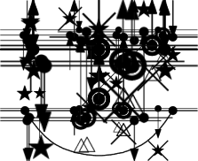
(a)

(b)

Figure 4: The probability that $x$ and $y$ are in distinct active runs in a conforming random situation is: (a) $3/4$, (b) $1/2$.

Let $(x,y)$ be a $k$-free sensitive pair contained in a cycle $W$ of $F$, and let the internal vertices of $xWy$ which are not heads of $\Delta$ be denoted by $x_{1},\dots,x_{k}$. Suppose that $(x,y)$ is of type (a); say, $x,y\in\Delta^{1}$. The active runs of $x$ and $y$ with respect to $\sigma$ will be separated if we require that at least one of $x_{1},x_{2},...,x_{k}$ is the tail of an arc of $\vec{\sigma}$, which happens with probability $1-(1/2)^{k}$. The same computation applies to a sensitive pair of type (b).

Now suppose that $(x,x)$ is sensitive of type (c), i.e., $x$ is the only member of $\Delta^{1}$ belonging to an odd cycle $W$ of length $\ell$. If some vertex of $W$ is the tail of an arc of $\vec{\sigma}$, then $x$ will be added in Phase 1 with probability $1/2$ as usual. It can happen, however (with probability $1/2^{\ell-1}$), that all the vertices of $W$ are heads in $\vec{\sigma}$, in which case $\Phi(V(W))$ is one of $\ell$ maximum independent sets in $W$. If this happens, $x$ will be added to $I$ with probability $1/2\cdot(\ell-1)/\ell\geq 2/5$ rather than $1/2$; this results in a reduction in $\mathbf{P}(\Gamma(\Delta))$ of at most $1/5\cdot 1/2^{\ell-1}\cdot 1/2^{w(\Delta)}$.

Finally, let us consider the situation where $u\in\Delta^{3}$ and the feasible run containing $u$ is cyclic, that is, the case where every vertex in $C_{u}$ is feasible. If $Z$ is even, then this has no effect as $u$ is still added in Phase 3 with probability $1/2$. If $Z$ is odd, then $u$ is added in Phase 3 with probability at least $2/5$ instead. Thus, if the probability of all vertices in $C_{u}$ being feasible is $q(\Delta)$, then the resultant loss of probability from $\mathbf{P}(\Gamma(\Delta))$ is at most $q(\Delta)/(5\cdot 2^{w(\Delta)})$.

Putting all this together gives:

$$\mathbf{P}(\Gamma(\Delta))\geq\left(1-\sum_{i=1}^{\ell}\frac{1}{2^{x_{i}}}-\sum_{i=1}^{c}\frac{1}{5\cdot 2^{y_{i}}}-\frac{q(\Delta)}{5}\right)\cdot\frac{1}{2^{w(\Delta)}}$$

as required. ∎

We remark that by a careful analysis of the template in question, it is sometimes possible to obtain a bound better than that given by Lemma 7; however, the latter bound will usually be sufficient for our purposes.

A template without any sensitive pairs is called weakly regular. If a weakly regular template $\Delta$ has $q(\Delta)=0$, then it is regular. By Lemma 7, if $\Delta$ is a regular template, then $\mathbf{P}(\Gamma(\Delta))\geq 1/2^{w(\Delta)}$. When using Lemma 7 in this way, we will usually just state that the template in question is regular and give its weight, and leave the straightforward verification to the reader.

The analysis is often more involved if sensitive pairs are present. To allow for a brief description of a template $\Delta$, we say that $\Delta$ is covered (in $G$) by ordered pairs of vertices $(x_{i},y_{i})$, where $i=1,\dots,k$, if every sensitive pair of $\Delta$ is of the form $(x_{i},y_{i})$ for some $i$. In most cases, our information on the edge set of $G$ will only be partial; although we will not be able to tell for sure whether any given pair of vertices is sensitive, we will be able to restrict the set of possibly sensitive pairs.

For brevity, we also use $(x,y)^{\ell}$ to denote an $\ell$-free pair of vertices $(x,y)$. Thus, we may write, for instance, that a template $\Delta$ is covered by pairs $(x,y)^{2}$ and $(z,z)^{4}$. By Lemma 7, we then have $\mathbf{P}(\Gamma(\Delta))\geq 1/2^{w(\Delta)}\cdot(1-1/4-1/80)$.

In some cases, the structure of $G$ may make some of the symbols in a diagram redundant. For instance, consider the diagram in Figure 5(a) and let $R_{1}$ be the event corresponding to the associated template $\Delta_{1}$. Since the weight of $\Delta_{1}$ is 4, Lemma 7 implies a lower bound for $\mathbf{P}(R_{1})$ which is slightly below $1/16$. However, if we happen to know that the mate of $u_{+}$ is $v_{-}$, then we can remove the symbol at $({u}_{+})^{\prime}$; the resulting diagram encodes the same event and comes with a better bound of $1/8$. We will describe this situation by saying that the symbol at $({u}_{+})^{\prime}$ in the diagram for $\Delta_{1}$ is removable (under the assumption that $({u}_{+})^{\prime}=v_{-}$).

(a) $\Delta_{1}$.

(b) $\Delta_{2}$.

Figure 5: The symbol at $({u}_{+})^{\prime}$ in the diagram defining the template $\Delta_{1}$ becomes removable if we add the assumption that $({u}_{+})^{\prime}=v_{-}$.

We extend the terminology used for templates to events defined by templates. Suppose that $\Delta$ is a template in $G$. The properties of $\Gamma(\Delta)$ simply reflect those of $\Delta$. Thus, we say that the event $\Gamma(\Delta)$ is regular (weakly regular) if $\Delta$ is regular (weakly regular), and we set $q(\Gamma(\Delta))=q(\Delta)$. A pair of vertices is said to be $k$-free for $\Gamma(\Delta)$ if it is $k$-free for $\Delta$; $\Gamma(\Delta)$ is covered by a set of pairs of vertices if $\Delta$ is.

4 Events forcing a vertex

In this section, we build up a repertoire of events forcing the distinguished vertex $u$. (Recall that $u$ is forced by an event $\Gamma$ if $u$ is contained in $I(\sigma)$ for every situation $\sigma\in\Gamma$.) In our analysis, we will distinguish various cases based on the local structure of $G$ and show that in each case, the total probability of these events (and thus the probability that $u\in I$) is large enough.

Suppose first that $\sigma$ is a situation for which $u$ is active. By the description of Algorithm 1, we will have $u\in I$ if either both $u_{+}$ and $u_{-}$ are inactive, or $u\in\sigma^{1}$. Thus, each of the templates $E^{0},E^{-},E^{+},E^{\pm}$ represented by the diagrams in Figure 6 defines an event which forces $u$. These events (which will be denoted by the same symbols as the templates, e.g., $E^{0}$) are pairwise disjoint. Observe that by the assumption that $G$ is simple and triangle-free, each of the diagrams is valid in $G$.

(a) Template $E^{0}$.

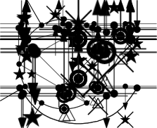
(b) Template $E^{-}$.

(c) Template $E^{+}$.

(d) Template $E^{\pm}$.

Figure 6: Some templates defining events which force $u$.

It is not difficult to estimate the probabilities of these events. The event $E^{0}$ is regular of weight 3, so $\mathbf{P}(E^{0})\geq 1/8=32/256$ by Lemma 7. Similarly, $E^{+}$ and $E^{-}$ are regular of weight 4 and have probability at least $16/256$ each. The weakly regular event $E^{\pm}$ has weight 4 and the only potentially sensitive pair is $(u,u)$. If the pair is sensitive, the length of $Z$ must be odd and hence at least 5; thus, the pair is 2-free. By Lemma 7,

$$\mathbf{P}(E^{\pm})\geq\frac{1}{16}\cdot\frac{19}{20}=15.2/256.$$

Note that if $Z$ has a chord (for instance, $uv$), then $E^{\pm}$ is actually regular, which improves the above estimate to $16/256$.

By the above,

$$\mathbf{P}(E^{0}\cup E^{+}\cup E^{-}\cup E^{\pm})\geq\frac{32+16+16+15.2}{256}=\frac{79.2}{256}.$$

These events cover most of the situations where $u\in I$. To prove Theorem 3, we will need to find other situations which also force $u$ and their total probability is at least about one tenth of the above. Although this number is much smaller, finding the required events turns out to be a more difficult task.

Since Figure 6 exhausts all the possibilities where $u$ is active, we now turn to the situations where $u$ is inactive.

Assume an event forces $u$ although $u$ is inactive. We find that if $u_{-}$ is active, then $u_{-2}$ must be added in Phase 1. If $u_{-}$ is inactive, then there are several configurations which allow $u$ to be forced, for instance if $u$ is added in Phase 3. However, the result also depends on the configurations around $u_{+}$ and $v$. We will express the events forcing $u$ as combinations of certain ‘primitive’ events.

Let us begin by defining templates $A,B,C_{1},C_{2},C_{3}$ (so called left templates). We remind the reader that the vertex $v$ is the mate of $u$. Diagrams corresponding to the templates are given in Figure 7:

template	heads of $\vec{\sigma}$	other conditions
$A$	$v,u_{-},u_{-2}$	$u_{-2}\in\sigma^{1}$
$B$	$v,({u}_{-})^{\prime}$	$u\in\sigma^{3}$
$C_{1}$	$v,({u}_{-})^{\prime}$	$u\notin\sigma^{3},({u}_{-})^{\prime}\in\sigma^{1}$
$C_{2}$	$v,({u}_{-})^{\prime},u_{-2}$	$u\notin\sigma^{3},({u}_{-})^{\prime}\notin\sigma^{1},u_{-2}\in\sigma^{1}$
$C_{3}$	$v,({u}_{-})^{\prime},u_{-2},({u}_{-3})^{\prime}$	$u\notin\sigma^{3},({u}_{-})^{\prime}\notin\sigma^{1},u_{-2}\notin\sigma^{1}$

In addition, for $P\in\left\{{A,B,C_{1},C_{2},C_{3}}\right\}$, the template $P^{*}$ is obtained by exchanging all ‘$-$’ signs for ‘$+$’ in this description. These are called right templates. In our diagrams, templates such as $A$ or $C_{1}$ restrict the situation to the left of $u$, while templates such as $A^{*}$ or $C_{1}^{*}$ restrict the situation to the right.

(a) Template $A$.

(b) Template $B$.

(c) Template $C_{1}$.

(d) Template $C_{2}$.

(e) Template $C_{3}$.

Figure 7: Left templates.

We also need primitive templates related to $v$ and its neighbourhood (upper templates), for the configuration here is also relevant. These are simpler (see Figure 8):

template	heads of $\vec{\sigma}$	other conditions
$D^{-}$	$v,v_{-},({v}_{+})^{\prime}$	$v_{-}\in\sigma^{1}$
$D^{0}$	$v,v_{-},v_{+}$	$v\notin\sigma^{1}$
$D^{+}$	$v,({v}_{-})^{\prime},v_{+}$	$v_{+}\in\sigma^{1}$

(a) Template $D^{-}$.

(b) Template $D^{0}$.

(c) Template $D^{+}$.

Figure 8: Upper templates.

We can finally define the templates obtained from the left, right and upper events as their combinations. More precisely, for $P,Q\in\left\{{A,B,C_{1},C_{2},C_{3}}\right\}$ and $R\in\left\{{D^{-},D^{0},D^{+}}\right\}$, we define $PQR$ to be the template $\Delta$ such that

$$\vec{\Delta} =\vec{P}\cup\vec{Q^{*}}\cup\vec{R},$$

$$\Delta^{1} =P^{1}\cup(Q^{*})^{1}\cup R^{1},$$

and so on for the other constituents of the template. The same symbol $PQR$ will be used for the event defined by the template. If the result is not a legitimate template (for instance, because an edge is assigned both directions, or because $u$ is required to be both in $\Delta^{3}$ and $\Delta^{\bar{3}}$), then the event is an empty one and is said to be invalid, just as if it were defined by an invalid diagram.

Let $\Sigma$ be the set of all valid events $PQR$ given by the above templates. Thus, $\Sigma$ includes, e.g., the events $AAD^{0}$ or $BC_{1}D^{+}$. However, some of them (such as $BC_{1}D^{+}$) may be invalid, and the probability of others will in general depend on the structure of $G$. We will examine this dependence in detail in the following section. It is not hard to check (using the description of Algorithm 1) that each of the valid events in $\Sigma$ forces $u$ and also that each of them is given by an admissible template, as defined in Section 3.

5 Analysis: $uv$ is not a chord

We are going to use the setup of the preceding sections to prove Theorem 3 for a cubic bridgeless graph $G$. Recall that $v$ denotes the vertex $u^{\prime}$ and $Z$ denotes the cycle of $F$ containing $u$. If we can show that $\mathbf{P}(u\in I)\geq 11/32$, then by Lemma 1, $\chi_{f}(G)\leq 32/11$ as required. Thus, our task will be accomplished if we can present disjoint events forcing the fixed vertex $u$ whose probabilities sum up to at least $11/32=88/256$. It will turn out that this is not always possible, which will make it necessary to use a compensation step discussed in Section LABEL:sec:phase5.

In this section, we begin with the case where $v$ is contained in a cycle $C_{v}\neq Z$ of $F$ (that is, $uv$ is not a chord of $Z$). We define a number $\varepsilon(u)$ as follows:

$$\varepsilon(u)=\begin{cases}1&\text{if $uv$ is contained in a 4-cycle,}\\ 0&\text{if $u$ has no $F$-neighbour contained in a 4-cycle intersecting $C_{v}$,}\\ -1&\text{otherwise}.\end{cases}$$

The vertices with $\varepsilon(u)=-1$ will be called deficient of type 0.

The end of each case in the proof of the following lemma is marked by $\blacktriangle$.

Lemma 8.

If $uv$ is not a chord of $Z$, then

$$\mathbf{P}(u\in I)\geq\frac{88+\varepsilon(u)}{256}.$$

Proof.

As observed in Section 4, the probability of the event $E^{0}\cup E^{-}\cup E^{+}$ is at least $64/256$. For the event $E^{\pm}$, we only get the estimate $\mathbf{P}(E^{\pm})\geq 15.2/256$, which yields a total of $79.2/256$.

Case 1.

The edge $uv$ is contained in two 4-cycles.

Consider the event $BBD^{0}$ of weight 5 (see the diagram in Figure 9(a)). We claim that $\mathbf{P}(BBD^{0})\geq 8/256$. Note that for any situation $\sigma\in BBD^{0}$, at least one of the vertices $v_{-}$, $v_{+}$ is added to $I$ in Phase 1. It follows that for any such situation, $u_{-}$ or $u_{+}$ is infeasible. Thus, $q(BBD^{0})=0$, and by Lemma 7,

$$\mathbf{P}(BBD^{0})\geq\frac{1}{2^{5}}=\frac{8}{256}.$$

Next, we use the event $ABD^{-}$ of weight 7 (see Figure 9(b)). Since $u_{-2}\in\sigma^{1}$ for any situation $\sigma\in ABD^{-}$, it is infeasible and hence $q(ABD^{-})=0$. Furthermore, $ABD^{-}$ contains no sensitive pair and thus it is regular. Lemma 7 implies that $\mathbf{P}(ABD^{-})\geq 2/256$. This shows that

$$\mathbf{P}(u\in I)\geq 89.2/256.$$

We remark that a further contribution of $2/256$ could be obtained from the event $AC_{1}D^{-}$, but it will not be necessary. $\blacktriangle$

(a) $BBD^{0}$.

(b) $ABD^{-}$.

Figure 9: The events used in Case 1 of the proof of Lemma 8.