A Short Note on Gaussian Process Modeling for Large Datasets using Graphics Processing Units

Abstract

The graphics processing unit (GPU) has emerged as a powerful and cost effective processor for general performance computing. GPUs are capable of an order of magnitude more floating-point operations per second as compared to modern central processing units (CPUs), and thus provide a great deal of promise for computationally intensive statistical applications. Fitting complex statistical models with a large number of parameters and/or for large datasets is often very computationally expensive. In this study, we focus on Gaussian process (GP) models – statistical models commonly used for emulating expensive computer simulators. We demonstrate that the computational cost of implementing GP models can be significantly reduced by using a CPU+GPU heterogeneous computing system over an analogous implementation on a traditional computing system with no GPU acceleration. Our small study suggests that GP models are fertile ground for further implementation on CPU+GPU systems.

, and

1 Introduction

Driven by the need for realistic real time computer graphics applications, graphics processing units (GPUs) now offer more computing power than central processing units (CPUs). This is accomplished with a large number of (relatively slow) processors that can simultaneously render complex 3D graphical applications by relying on parallelism. Modern GPUs can be programmed to execute many of the same tasks as a CPU. For tasks with efficient (primarily floating point) parallel implementations, GPUs have reduced execution time by an order of magnitude or more (Brodtkorb et al., 2010). Additionally, GPUs are extremely cost effective; delivering far more floating point operations per second (FLOPS) per dollar than multi-core CPUs. This provides a great deal of promise for general purpose computing on graphics processing units (GPGPU), and in particular for computationally intensive statistical applications (e.g., Zechner & Granitzer (2009); Lee et al. (2009)).

In this note, we explore the merits of heterogeneous computing (CPU+GPU) over traditional computing (CPU only) for fitting Gaussian process (GP) models. GP models are popular supervised learning models (Rasmussen & Williams, 2006), and are also used for emulating computer simulators which are too time consuming to run for real-time predictions (Sacks et al., 1989). Fitting a GP model with $n$ simulator runs requires the determinant and inverse computation of numerous $n\times n$ spatial correlation matrices. The computational costs of both the determinant and inverse are $O(n^{3})$, which become prohibitive for moderate to large $n$. We demonstrate that for moderate to large datasets (thousands of runs), the implementation on a heterogeneous system can be more than a hundred times faster. The tremendous speed-ups were achieved by leveraging NVIDIA’s compute unified device architecture (CUDA) toolkit (NVIDIA Corporation, 2010).

This note is intended as a “proof of concept” to demonstrate the tremendous time savings that can be achieved for statistical simulations by using GPUs. In particular we show that fitting GP models on a heterogeneous computing platform leads to significant time savings as compared to our previous CPU-only implementation.

The remainder of this note is organized as follows: Section 2 briefly reviews the basic formulation of the GP model. We also highlight the computationally intensive steps of the model fitting procedure in this section. Implementation details for both platforms (CPU + GPU and CPU-only) are discussed in Section 3. Comparisons are made via several simulations in Section 4, followed by discussion in Section 5. It is clear from this study that the efficiency, affordability, and pervasiveness of GPUs suggest that they should seriously be considered for intensive statistical computation.

2 Gaussian Process Model

GP models are commonly used for regression in machine learning, geostatistics and computer experiments. Here, we adopt terminology of computer experiments (Sacks et al., 1989). Denote the $i$-th input and output of the computer simulator by $x_{i}=(x_{i1},...,x_{id})$, and $y_{i}=y(x_{i})$, respectively. The simulator output, $y(x_{i})$, is modeled as

$$y(x_{i})=\mu+z(x_{i});\qquad i=1,...,n,$$ (1)

where $\mu$ is the overall mean, and $z(x_{i})$ is a GP with $E(z(x_{i}))=0$, $Var(z(x_{i}))=\sigma^{2}_{z}$, and Cov$(z(x_{i}),z(x_{j}))=\sigma^{2}_{z}R_{ij}$. Although there are several choices for $R$ (Santner et al., 2003), we use the power exponential correlation family

$$R_{ij}=\mbox{corr}(z(x_{i}),z(x_{j}))=\prod_{k=1}^{d}\exp\left\{-\theta_{k}|(x_{ik}-x_{jk})|^{p}\right\},\quad\mbox{ for all }\quad i,j,$$ (2)

where $\theta=(\theta_{1},...,\theta_{d})$ is the vector of hyper-parameters, and $p\in(0,2]$ is the smoothness parameter. The squared exponential $(p=2)$ correlation function is very popular and has good theoretical properties, however, the power exponential correlation function with $p<2$ is more stable in terms of near-singularity of $R$ (especially if the design points are very close, which can occur with large $n$ in small $d$ - dimensional space). We used $p=1.95$ for all illustrations in this note (Kaufman et al., 2011). Alternatively, a suitably chosen nugget with Gaussian correlation can be used (Ranjan et al., 2011) to avoid near-singularity. One could also use another correlation structure like Matérn (Stein, 1999; Santner et al., 2003), which is considered to be numerically more stable than power exponential correlation.

We implemented the maximum likelihood approach for fitting the GP model, which requires the estimation of the parameter vector $(\theta_{1},...,\theta_{d};\mu,\sigma^{2}_{z})$. The closed form estimators of $\mu$ and $\sigma^{2}_{z}$ are given by

$$\hat{\mu}(\theta)={({\bf 1_{n}}^{\prime}R^{-1}{\bf 1_{n}})}^{-1}({\bf 1_{n}}^{\prime}R^{-1}Y)\ \text{and}\ \hat{\sigma}^{2}_{z}(\theta)=\frac{(Y-{\bf 1_{n}}\hat{\mu}(\theta))^{\prime}R^{-1}(Y-{\bf 1_{n}}\hat{\mu}(\theta))}{n},$$ (3)

which are used to obtain the profile log-likelihood

$$-2\log L_{\theta}\propto\log(|R|)+n\log[(Y-{\bf 1_{n}}\hat{\mu}(\theta))^{\prime}R^{-1}(Y-{\bf 1_{n}}\hat{\mu}(\theta))],$$ (4)

for estimating the hyper-parameters $\theta=(\theta_{1},...,\theta_{d})$, where $|R|$ denotes the determinant of $R$.

The evaluation of $|R|$ and $R^{-1}(Y-{\bf 1_{n}}\hat{\mu}(\theta))$ for different values of $\theta$ is computationally expensive. One can save some computation time and increase numerical stability by using matrix factorization of $R$ (e.g., using LU, QR or Cholesky decomposition) along with solving the linear systems via back-solves to obtain $R^{-1}(Y-{\bf 1_{n}}\hat{\mu}(\theta))$. From an implementation viewpoint, the log-likelihood (4) consists of three computationally expensive components: (i) the evaluation of $R$, (ii) the factorization of $R$ and (iii) solving the linear systems via back-solves. The computational cost for the matrix factorization and back-solves are $O(n^{3})$ and $O(n^{2})$ respectively. Thus, the log-likelihood function evaluation is computationally expensive, specifically for large $n$.

The log-likelihood surface is sometimes bumpy near $\theta=0$ and often has multiple local optima (Yuan et al., 2008; Schirru et al., 2011; Kalaitzis & Lawrence, 2011; Petelin et al., 2011). This makes maximizing the likelihood challenging. For instance, Figure 1 presents contours of $-2\log L_{\theta}$ for a $30$-point, two-dimesional data set, where the inputs are generated using a maximin Latin hypercube design (LHD) in $[0,1]^{2}$, and the computer simulator outputs are obtained by evaluating the two-dimensional GoldPrice function (see Example 1 for more details on this test simulator).

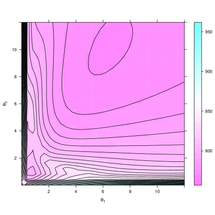
(a) $-2\log L_{\theta}$ surface for $(\theta_{1},\theta_{2})\in(0,12)^{2}$

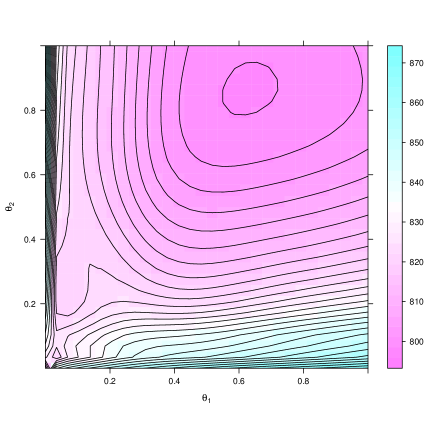
(b) $-2\log L_{\theta}$ surface zoomed in near $(\theta_{1},\theta_{2})=0$

Figure 1: Plots of $-2\log L_{\theta}$ for the GoldPrice function (Example 1) with $n=30$ points chosen using a random maximin LHD.

The log-likelihood surface in Figure 1 contains multiple local minima near $\theta=0$. Though not very clear from Figure 1(b), more local minima are found by enlarging the region near $\theta=0$. A good optimization algorithm that guarantees the global optimum of such an objective function would require numerous function evaluations. Evolutionary algorithms like genetic algorithm (Ranjan et al., 2008, 2011) and particle swarm optimization (Petelin et al., 2011) are commonly used for optimizing the log-likelihood of the GP models. A multi-start gradient based optimization approach might be faster but would require careful selection of the starting points to achieve the global minimum of $-2\log L_{\theta}$. Once a sufficiently large number of starting points are chosen, a gradient based optimization is also likely to involve a large number of evaluations of the likelihood.

The large number of likelihood evaluations, no matter what approach is taken to search for the MLEs, means that efficient ways to evaluate the likelihood will be very important.

3 Implementation of GP on CPUs and GPUs

In this section, we discuss the implementations of GP fitting algorithms in the two computing environments. As in Ranjan et al. (2008, 2011), we use a genetic algorithm (GA) for minimizing $-2\log L_{\theta}$. Other optimizers might use different strategies, but all approaches require numerous evaluation of (4).

Our implementation of computing $-2\log L_{\theta}$ requires one evaluation of $R$, one Cholesky decomposition of $R$ and seven back-solves involving the Cholesky factors. The version of GA implemented here for optimizing the log-likelihood uses $2000$ evaluations of $-2\log L_{\theta}$. Thus, the GP model fitting procedure requires $2000$ evaluations of $R$, $2000$ Cholesky decompositions and $14000$ back-solves. Furthermore, the GP model predictions on a set of $N$ test points are obtained using the estimated parameters with one evaluation of $R$, one Cholesky decomposition and $2N+6$ back-solves. Thus, fitting a GP model and obtaining model predictions are computationally expensive, and this paper advocates the use of GPUs to reduce the computational burden.

The heterogeneous (CPU+GPU) workstation for this study includes two moderately high-end consumer grade components each costing approximately $200: a Intel Core i5 750 CPU and a NVIDIA GTX 260 (core 216) GPU. The Intel CPU is capable of 4 flops per clock cycle $\times$ 4 cores $\times$ 2.66 gigaHertz per core = 42.58 gigaFlops per cycle (Intel Corporation, 2011). The NVIDIA GPU is capable of 3 flops per clock cycle $\times$ 216 cores $\times$ 1.547 gigaHertz per core = 1002 gigaFlops per cycle (Barrachina et al., 2009), roughly 24 times more than the Intel Core i5 processor. The workstation used for comparison is a dual-socket quad-core AMD Opteron 2352 with 32 GB of RAM running Matlab version R2009b. This hardware is slightly older, but is workstation class instead of consumer class, has more RAM and twice as many CPU cores.

CPU implementation. Most personal computers available now have multi-core processors. For example, the somewhat high-end consumer-grade AMD FX-8120 has 8 cores. We used a dual-socket quad core AMD Opteron 2352 based workstation, giving 8 cores in total. The CPU implementation was written in Matlab, making use of several built-in functions (e.g., matrix factorization routines, backslash operator for back-solving linear systems) that are linked to compiled high performance subroutines written in Fortran or C. The Cholesky decomposition was used for computing both the determinant and the inverse of $R$ (via solving linear systems). The Matlab (CPU) code did not contain specialized parallelization commands. However, the Matlab session used all 8 cores through its intermal math routines.

CPU+GPU implementation. The most popular GPGPU platform is that of a Intel or AMD x86 CPU and a Nvidia GPU. This is the platform that was adopted for this study - an Intel core i5 750 quad core CPU and Nvidia GTX 260 GPU. We used the Nvidia GPGPU software development kit (CUDA 2.3) to implement the Gaussian process model on this system. As part of that implementation we rewrote our Matlab code in the C for CUDA programming language to enable general purpose computation on the GPU. The free libraries CUDA basic linear algebra subroutines (CUBLAS) (NVIDIA Corporation, 2009) and CULATools (EM Photonics and NVIDIA Corporation, 2009) were used for executing the most computationally expensive steps of the GP model on the GPU. CULATools is a proprietary library with a free version that provides popular linear algebra operations for NVIDIA GPUs. Because the Cholesky decomposition routine was not part of the free CULATools library, the free (but closed source) LU decomposition (culaDeviceSgetrf) was used instead. Though we are not certain due to the proprietary nature of CULATools, we believe the GPU LU decomposition is parallelized in a block-based manner similar to the freely available SCALAPACK version for CPUs (Choi et al., 1992).

We explicitly used the GPU for evaluation of correlation matrix $R$ using a custom GPU kernel (C for CUDA function), LU decomposition of $R$ (CULATOOLS library), all linear algebraic operations including the back-solves (CUBLAS library), and a few other custom C for CUDA functions in order to minimize the transfer of data to and from the GPU. The computation of $R$ requires $d\cdot n(n-1)/2$ evaluations of $-\theta_{k}|(x_{ik}-x_{jk})|^{1.95}$ all of which are mutually independent and can be executed in parallel.

Note that no task parallelization (e.g., multiple evaluation of the likelihood at different parameter values) was performed in this implementation. Evaluating the likelihood for numerous parameters simultaneously seems a natural approach to parallelizing a GP model, however this type of parallelism was not possible because only one kernel could have been executed at a time. If we had access to a more advanced GPU (e.g., GF100 series or newer), executing some of these computationally intensive steps in a task parallel manner (using concurrent kernel execution) could potentially lead to even more time savings.

To summarize, we used the GPU for all linear algebra operations and building the correlation matrix $R$. The CPU was used for data input/output and process control. Additional execution configurations could have been tuned to optimize the performance of GPUs (Archuleta et al., 2009). However the aim of this study is not to achieve the highest performance possible for these models and procedures; but rather to explore the use of a GPU as a co-processor that can lead to significant time savings at a reasonable cost.

4 Examples

In this section, we use simulated examples to compare the results obtained from the two implementations of the GP model. Throughout this note, the CPU implementation of the methodology in Matlab is referred to as CPU implementation and the mixed system (CPU + GPU) implementation (in C based language called CUDA) is referred to as CUDA implementation. Our CUDA implementation enforces single precision floating-point arithmetic and uses LU instead of Cholesky decomposition of the correlation matrices $R$.

For fair comparison of the results, both implementations used exactly the same input data and the number of likelihood evaluations in the optimization procedure. The design points, $\bm{x}=(x_{1},...,x_{n})$, were generated using a maximin Latin-hypercube scheme. For efficient distribution of the data to the processors in the CUDA implementation, we used powers of $2$ for $n$, however, other values of $n$ can also be considered in our implementations (e.g., we used $n=4064$ in Example 2). Simulations with $n>4070$ were not considered here because of a restriction within the CUBLAS library (version 2.3). In the most recent CUBLAS release (3.0) this restriction has been relaxed, allowing for much larger matrices to be considered in future applications.

As pointed out in Sections 2 and 3, the challenge of effectively maximizing the likelihood for a GP model leads to algorithms that repeatedly evaluate the likelihood. In the examples considered in this section, a genetic algorithm with 20 generations and a population of 100 solutions leading to 2,000 likelihood evaluations, was used.

Example 1. Suppose the emulator outputs are generated from the $\log$ of the 2-dimensional Goldstein-Price function (Törn & Žilinskas, 1979). Designs of different sizes, $n=2^{k}$ for $k=4,5,...,9$, were used to fit the GP model. The reason for not using larger designs in this simulation study is discussed in Section 5. Table 1 shows the parameter estimates, optimized value of $-2\log(L_{\theta})$ as in (4), sum of squared prediction error ($SSPE=\sum_{i=1}^{1000}(y_{i}-\hat{y}_{i})^{2}$), and total runtime of the code (i.e., fitting the GP model and computing SSPE). The SSPE is calculated over a fixed test set, which is a maximin LHD chosen independent to the design used for model fitting. Both CPU and CUDA implementations used the same training and test datasets. A slight randomness (or variation) in these performance measures is introduced due to the stochasticity of the genetic algorithm used for optimizing the likelihood. To reduce the variation, the results in Table 1 are averaged over ten simulations. For each replication of the experiment a different design (training dataset for fitting the GP model) was chosen.

Table 1: Simulation results for Goldstein-Price function, averaged over 10 replications.

CPU implementation

$n$ Time(sec) $-2logL_{\theta}$ $\hat{\mu}$ $\hat{\sigma}^{2}_{z}$ SSPE 16 0.91 55.95 9.80 7.09 1158.89 32 3.30 130.98 9.36 5.19 860.47 64 12.90 286.46 9.47 5.31 219.73 128 51.45 541.83 9.58 4.77 131.87 256 206.18 1186.40 9.31 3.17 28.84 512 911.93 2287.88 9.41 4.91 11.91

CUDA implementation

$n$ Time(sec) $-2logL_{\theta}$ $\hat{\mu}$ $\hat{\sigma}^{2}_{z}$ SSPE 16 2.26 56.85 9.83 7.19 1188.21 32 4.94 130.48 9.47 5.25 831.98 64 5.50 285.47 9.43 4.61 225.83 128 7.25 536.32 9.54 3.61 134.15 256 9.88 1207.87 9.54 4.73 40.56 512 20.75 2321.21 9.59 4.79 14.38

It is clear from Table 1 that the optimized value of the profile log-likelihood ($-2\log L_{\theta}$), $\hat{\mu}$, $\hat{\sigma}^{2}_{z}$ and SSPE from the two implementations are comparable within each sample size. The discrepancy between the results of these two implementations may be partially explained by the fact that single precision floating point operations were used in CUDA as compared to double precision calculations in Matlab. See Section 5 for further discussion.

While the discrepancies in Table 1 suggest that single-precision arithmetic on the GPU may not always yield exact optima, we stress that the most difficult part of the likelihood optimization is finding the right neighbourhood of a good optimum. Short double-precision runs on the CPU may be used to refine the CUDA results.

The column “Time(sec)” in Table 1 shows that as $n$ increases the CUDA implementation significantly outperforms the CPU implementation. For $n=512$, on average CPU implementation takes more than $15$ minutes but CUDA implementation requires roughly $21$ seconds.

Example 2. Consider the 6-dimensional Hartman function (Törn & Žilinskas, 1979) for generating the simulator outputs. Since the input space is six dimensional, we considered relatively large designs with $n=2^{6},2^{8},2^{10}$ and $4064$ ($n>4070$ is not allowed due to CUBLAS restrictions) to fit the GP model, and the SSPE was calculated over 1000 points chosen using a maximin LHD. Table 2 summarizes the simulation results.

Table 2: Simulation results for Hartman function, averaged over 10 replications (except *, one replication)

CPU implementation

$n$ Time(s) $-2logL_{\theta}$ $\hat{\mu}$ $\hat{\sigma}^{2}_{z}$ SSPE 64 32.32 125.94 0.1771 0.1403 77.4160 256 514.43 610.25 0.1105 0.1164 27.4311 1024 13325.86 2491.97 0.0609 0.0970 5.6504 4064 *161925.05 *8044.80 *0.0485 *0.0824 *0.5320

CUDA implementation

$n$ Time(s) $-2logL_{\theta}$ $\hat{\mu}$ $\hat{\sigma}^{2}_{z}$ SSPE 64 9.45 103.70 0.1238 0.2989 91.7860 256 16.58 547.10 0.1397 0.1746 31.4641 1024 96.19 2665.58 0.1192 0.1390 4.3850 4064 1059.71 8698.28 0.0803 0.0700 0.5314

Similar to Example 1, the results are averaged over 10 simulations. One exception is CPU with $n=4064$: a single run took almost 45 hours, and thus we did not perform 10 simulations. Table 2 shows that the CUDA implementation achieves computation time savings of up to a factor of 150 ($n=4064$).

5 Discussion

This note illustrates that GPU parallelization can significantly reduce the computational burden in fitting GP models. The largest improvements are evident in the most difficult problems (e.g., from 45 hours to 18 minutes in Example 2, $n=4064$ case). These dramatic savings suggest that more complete implementations of GP models on GPU platforms deserve further study.

Although this article focuses on speedups due to hardware, there are other approaches for estimation of GP models with large sample sizes. For instance, ad-hoc methods have been proposed which modify the correlation function and give sparse correlation matrices, facilitating faster computation of the inverses and determinants (e.g., Furrer et al. (2006), Stein (2008)). However, it seems quite plausible that efficiencies realized by a GPU+CPU approach would also benefit these sparse approximations.

A number of design choices in the experiments merit commentary. In Example 1, the reason for not considering $n=2^{10}$ or larger is that the correlation matrices are near-singular. Although choice of the exponent in the correlation matrix $R$, set at $p=1.95$, substantially reduces the chance of getting near-singular correlation matrices, this is still a problem for large $n$ in the two-dimensional problem. We did not want to further lower the value of $p$, as it would affect the smoothness of the GP fit. Alternatively, a nugget based approach (Ranjan et al., 2011) can be used to implement the GP model with large datasets. It is expected that the runtime of the model fitting procedure would not change significantly with $p$, except when the correlation matrix becomes sparse.

As noted in Section 4, MLEs obtained by the CPU+GPU implementation differed somewhat from those found by the CPU implementation. A significant reason for this is the use of single-precision arithmetic in the GPU code. These estimates could be refined by a short run of double-precision CPU code. Since this refinement might involve 10 or 20 likelihood evaluations, a small fraction of the 2000 necesary to find a good solution, we have not included this effect in our studies.

There are a number of specific functions for high-level software packages like Matlab and R that leverage GPUs and can be used to improve existing codes. For instance, our CPU implementation can be improved by using Jacket (AccelerEyes, 2011) and GPUlib (Tech-X Corporation, 2011). This approach was not taken for this study as GPUs were not available in our cluster, and Matlab was not available on our heterogenous computing system. Similarly, GPUtools is a library for GPU accelerated routines in R (Buckner et al., 2010).

Though not discussed here, it is possible to make use of more than one CPU and as many as three or four GPUs in one application/system, if there are available GPU slots. In fact, cutting edge research is currently being done using multiple GPUs coupled by an extremely fast interconnect (Infiniband) (QLogic Corporation, 2011). Even more processing power can be achieved by creating a cluster of CPU+GPU systems coupled over a network, like the second and fourth fastest supercomputers in the world (as of June 2011), the Chinese Tianhe-1A and Nebulae (Top500.org, 2011). Developing algorithms to execute in parallel across numerous processors is not a task that is frequently undertaken by statisticians. However, parallel computing, GPU co-processing, and heterogeneous computing techniques can become popular in the near future for computationally intensive statistical computing applications because of the promise of heterogeneous computing and likely changes to CPU architectures (Brodtkorb et al., 2010).

References

- (1)
- AccelerEyes (2011) AccelerEyes (2011), ‘Jacket website’. http://www.accelereyes.com/products/jacket.
- Archuleta et al. (2009) Archuleta, J., Cao, Y., Scogland, T. & Feng, W. (2009), ‘Multi-dimensional characterization of temporal data mining on graphics processors’, Proceedings of the 2009 IEEE International Symposium on Parallel & Distributed Processing 00, 1–12.
- Barrachina et al. (2009) Barrachina, S., Castillo, M., Igual, F., Mayo, R., Quintana-Ortí, E. & Quintana-Ortí, G. (2009), ‘Exploiting the capabilities of modern gpus for dense matrix computations’, Concurrency and Computation: Practice and Experience 21(18), 2457–2477.
- Brodtkorb et al. (2010) Brodtkorb, A. R., Dyken, C., Hagen, T. R., Hjelmervik, J. M. & Storaasli, O. O. (2010), ‘State-of-the-art in heterogeneous computing’, Scientific Programming 18, 1–33.
- Buckner et al. (2010) Buckner, J., Seligman, M. & Wilson, J. (2010), ‘Gputools’, http://cran.r-project.org/web/packages/gputools/index.html.
- Choi et al. (1992) Choi, J., Dongarra, J., Pozo, R. & Walker, D. (1992), Scalapack: A scalable linear algebra library for distributed memory concurrent computers, in ‘Frontiers of Massively Parallel Computation, 1992., Fourth Symposium on the’, IEEE, pp. 120–127.
- EM Photonics and NVIDIA Corporation (2009) EM Photonics and NVIDIA Corporation (2009), ‘Culatools basic: GPU-accelerated LAPACK’, http://www.culatools.com.
- Furrer et al. (2006) Furrer, R., Genton, M. G. & Nychka, D. (2006), ‘Covariance tapering for interpolation of large spatial datasets’, Journal of Computational and Graphical Statistics 15, 502–523.
- Intel Corporation (2011) Intel Corporation (2011), ‘Intel microprocessor export compliance metrics’. http://www.intel.com/support/processors/sb/CS-023143.htm.
- Kalaitzis & Lawrence (2011) Kalaitzis, A. A. & Lawrence, N. D. (2011), ‘A simple approach to ranking differentially expressed gene expression time courses through gaussian process regression’, BMC Bioinformatics 12, 180.
- Kaufman et al. (2011) Kaufman, C. G., Bingham, D., Habib, S., Heitmann, K. & Frieman, J. A. (2011), ‘Efficient emulators of computer experiments using compactly supported correlation functions, with an application to cosmology’, The Annals of Applied Statistics 5(4), 2470 – 2492.
- Lee et al. (2009) Lee, A., Yau, C., Giles, M. B., Doucet, A. & Holmes, C. C. (2009), ‘On the utility of graphics cards to perform massively parallel simulation of advanced Monte Carlo methods’. arXiv:0905.2441v3.
- NVIDIA Corporation (2009) NVIDIA Corporation (2009), ‘CUBLAS Library, Version 2.3’, http://developer.nvidia.com/object/gpucomputing.html.
- NVIDIA Corporation (2010) NVIDIA Corporation (2010), ‘CUDA Toolkit’, http://developer.nvidia.com/cuda-toolkit.
-
Petelin et al. (2011)
Petelin, D., Filipič, B. & Kocijan, J. (2011), Optimization of gaussian process models with
evolutionary algorithms, in ‘Proceedings of the 10th international
conference on Adaptive and natural computing algorithms - Volume Part I’,
ICANNGA’11, Springer-Verlag, Berlin, Heidelberg, pp. 420–429.
http://dl.acm.org/citation.cfm?id=1997052.1997098 - QLogic Corporation (2011) QLogic Corporation (2011), ‘Maximizing gpu cluster performance: Truescale infiniband accelerates gpu cluster’, Whitepaper: http://www.qlogic.com/Resources/Documents/WhitePapers/InfiniBand/Maximizing_GPU_Cluster_Performance.pdf.
- Ranjan et al. (2008) Ranjan, P., Bingham, D. & Michailidis, G. (2008), ‘Sequential experiment design for contour estimation from complex computer codes’, Technometrics 50(4), 527–541.
- Ranjan et al. (2011) Ranjan, P., Haynes, R. & Karsten, R. (2011), ‘A computationally stable approach to gaussian process interpolation of deterministic computer simulation data’, Technometrics 53(4), 366–378.
- Rasmussen & Williams (2006) Rasmussen, C. E. & Williams, C. K. I. (2006), Gaussian Processes for Machine Learning, The MIT Press, Cambridge.
- Sacks et al. (1989) Sacks, J., Welch, W., Mitchell, T. & Wynn, H. (1989), ‘Design and analysis of computer experiments’, Statistical Science 4(4), 409–435.
- Santner et al. (2003) Santner, T. J., Williams, B. & Notz, W. (2003), The design and analysis of computer experiments, Springer Verlag, New York.
- Schirru et al. (2011) Schirru, A., Pampuri, S., Nicolao, G. D. & McLoone, S. (2011), ‘Efficient marginal likelihood computation for gaussian processes and kernel ridge regression’. arXiv:1110.6546v1.
- Stein (1999) Stein, M. L. (1999), Interpolation of spatial Data: some theory for kriging, Springer, New York.
- Stein (2008) Stein, M. L. (2008), ‘A modeling approach for large spatial datasets’, Journal of Korean Statistical Society 37, 3–10.
- Tech-X Corporation (2011) Tech-X Corporation (2011), ‘Gpulib website’. http://www.txcorp.com/products/GPULib.
- Top500.org (2011) Top500.org (2011), ‘Top500 supercomputer sites’, http://www.top500.org/lists/2011/06.
- Törn & Žilinskas (1979) Törn, A. & Žilinskas, A. (1979), Global Optimization, Springer Verlag, Berlin.
-
Yuan et al. (2008)
Yuan, J., Wang, K., Yu, T. & Fang, M. (2008), ‘Reliable multi-objective optimization of high-speed
wedm process based on gaussian process regression’, International
Journal of Machine Tools and Manufacture 48(1), 47 – 60.
http://www.sciencedirect.com/science/article/pii/S0890695507001265 - Zechner & Granitzer (2009) Zechner, M. & Granitzer, M. (2009), ‘Accelerating k-means on the graphics processor via CUDA’, First International Conference on Intensive Applications and Services pp. 7–15.