A photometric and spectroscopic study of NSVS 14256825: the second sdOB+dM eclipsing binary

Abstract

We present an analysis of UBVR_CI_CJH photometry and phase-resolved optical spectroscopy of NSVS 14256825, an HW Vir type binary. The members of this class consist of a hot subdwarf and a main-sequence low-mass star in a close orbit ($P_{\rm orb}\sim 0.1$ d). Using the primary-eclipse timings, we refine the ephemeris for the system, which has an orbital period of 0.11037 d. From the spectroscopic data analysis, we derive the effective temperature, $T_{1}=40000\pm 500$ K, the surface gravity, $\log g_{1}=5.50\pm 0.05$, and the helium abundance, $n(\rm He)$/$n(\rm H)=0.003\pm 0.001$, for the hot component. Simultaneously modelling the photometric and spectroscopic data using the Wilson-Devinney code, we obtain the geometrical and physical parameters of NSVS 14256825. Using the fitted orbital inclination and mass ratio ($i=82\aas@@fstack{\circ}5\pm 0\aas@@fstack{\circ}3$ and $q=M_{2}/M_{1}=0.260\pm 0.012$, respectively), the components of the system have $M_{1}=0.419\pm 0.070~{}\rm M_{\odot}$, $R_{1}=0.188\pm 0.010~{}\rm R_{\odot}$, $M_{2}=0.109\pm 0.023~{}\rm M_{\odot}$, and $R_{2}=0.162\pm 0.008~{}\rm R_{\odot}$. From its spectral characteristics, the hot star is classified as an sdOB star.

1 Introduction

HW Virginis (HW Vir) systems consist of a subdwarf B or OB (sdB or sdOB; hereafter referred to as sdB) plus a main sequence star, which form an eclipsing pair in a compact orbit, $P_{\rm orb}\sim 0.1$ d (Heber, 2009). These systems are believed to evolve through a common envelope phase when the primary (sdB) is a red giant. During this stage, the secondary star (dM) spirals in towards the primary one and the potential gravitational energy released is absorbed by the envelope, which is subsequently ejected (Taam & Ricker, 2010). The final separation between the dM and the sdB stars depends on the initial mass ratio of the binary and the initial separation.

sdB stars consist of a helium-burning core covered by a thin hydrogen-dominated envelope. The atmosphere abundance is normally $n$(He)$/n$(H) $\sim$ 0.01, the effective temperatures are in the range of 22000–37000 K, and the logarithmic surface gravities are normally between 5.2 and 5.7. They populate a narrow strip on the extreme horizontal branch (EHB) in the Hertzsprung-Russell diagram. The single-star stellar evolution predicts a narrow mass range: 0.46 – 0.50  M_⊙ (Dorman et al. 1993). On the other hand, models based on binary evolution predict a broader range of masses, from 0.3 to 0.8  M_⊙ (Han et al. 2003). Hence an important step in understanding the origin of sdB stars is the determination of their mass distribution. A recent review of sdB stars is presented by Heber (2009).

There are currently ten members of the HW Vir class, whose main features are summarised in Table 1. Among them, NSVS 14256825 (2MASS J2020+0437; hereafter referred to as NSVS 1425) is one of the least studied. It was discovered in the public data from the Northern Sky Variability Survey (Wozniak et al., 2004). The sole information on this system comes from the photometric data by Wils, Giorgio & Sebastián (2007). These authors obtained B, V, and I_C photometric light curves. The main parameters obtained by Wils et al. (2007) are listed in Table 1.

Table 1: The currently known sdB$+$dM eclipsing binaries.

Name	$T_{1}$	$M_{1}$	$M_{2}$	$R_{1}$	$R_{2}$	$\log g_{1}$	Period	Refs.	Notes
	(K)	($\rm M_{\sun}$)	($\rm R_{\sun}$)	($\rm R_{\sun}$)	($\rm R_{\sun}$)		(d)
AA Dor	42000	0.33/0.47	0.064/0.079	0.179/0.20	0.097/0.108	5.46	0.261	,,	,
		0.25	0.054	0.165	0.089
NSVS 14256825	40000	0.419	0.109	0.190	0.151	5.50	0.11037	this work	,
	–	0.46	0.21	–	–	–	0.11040
PG 1336$-$018	31300	0.389	0.110	0.150	0.160	5.60	0.10102		,
	32740	0.459	–	–	–	–	–
2M 1533+3759	30400	0.377	0.113	0.166	0.152	5.58	0.16177		,
2M 1938$+$4603	29564	0.48	0.12	–	–	5.425	0.12576		,
HS 0705+6700	28800	0.48	0.13	0.230	0.186	5.40	0.09565		,
PG 1241$-$084	28488	0.48	0.14	0.176	0.180	5.63	0.11676
HS 2231+2441	28370	0.47/0.499	0.075/0.072	0.250	0.127	5.39	0.11059		,
SDSSJ0820$+$0008	26700	0.25/0.47	0.068/0.045	–	–	5.48	0.096		,
BUL SC16 335	–	–	–	–	–	–	0.12505

Heber (2009);  Klepp & Rauch (2011);  Hilditch et al. (2003);  Rucinski (2009);  Wils et al. (2007);  Vuĉković et al. (2009);  Charpinet et al. (2008);  For et al. (2010);  Østensen et al. (2010);  Drechsel et al. (2001);  Wood & Saffer (1999);  Østensen et al. (2007);  Geier et al. (2011);  Polubek et al. (2007);  Light Curves;  Spectroscopy;  Asteroseismology.

In this paper, we report on multi-band photometry and phase-resolved optical spectroscopy of NSVS 1425. We present an improved solution for its geometrical and physical parameters and discuss these results in the context of HW Vir systems and their evolution.

2 Observations and Data Reduction

2.1 Optical and near infrared photometry

The observations were carried out using the Observatório do Pico dos Dias (OPD/LNA) facilities, in Brazil. Photometric data in the U, B, V, R_C, I_C, J, and H bands were obtained from July to November, 2010. Optical observations were performed using a CCD camera attached to the 0.6-m IAG telescope. Near infrared photometry data were collected by means of a CamIV imager attached to the 1.6-m Perkin-Elmer telescope.

The procedure to remove undesired effects from the CCD data included obtaining $\sim$100 bias frames and $\sim$30 dome flat-field images for each night of observations. The NIR flat-field images were produced using separate sequences of $30$ “on” and $30$ “off” exposures. The resulting of the “on” image minus “off” image was used as the master flat-field image. Table 2 summarises the characteristics of the data collected for NSVS 1425. In this table, $N$ is the number of individual images obtained with the integration time t_exp.

The preparation of the CCD data was performed using standard IRAF tasks (Tody, 1993) and consisted of subtracting a master median bias image from each program image, and then dividing the result by a normalised flat-field frame. In the J and H bands, additional steps of linearization and sky subtraction from dithered images were used in the preparation of the data. For both optical and infrared data, differential photometry was used to obtain the relative fluxes between the target and a set of constant flux stars in the field of view. As the NSVS 1425 field is not crowded, the extraction of the fluxes was carried out using aperture photometry. Figure 1 shows a finding chart for NSVS 1425 with a reference star and a number of additional comparison stars adopted for differential photometry. Photometric standard stars were observed each night in order to calibrate the optical data. The NIR calibration is directly provided by the 2MASS catalogue magnitudes for the reference and comparison stars. Figure 2 shows a sample of calibrated light curves folded on the NSVS 1425 orbital period.

As can be seen in Figure 2, the light curves of NSVS 1425 show a prominent reflection effect, which increases towards longer wavelengths. The depth of the primary eclipse is $\sim$0.7 mag and does not change significantly with wavelength, while the depth of the secondary eclipse increases towards longer wavelengths, from $\sim$0.1 mag in the U band to $\sim$0.18 mag in the H band. Table 3  shows the apparent magnitudes for NSVS 1425 at primary and secondary minima.

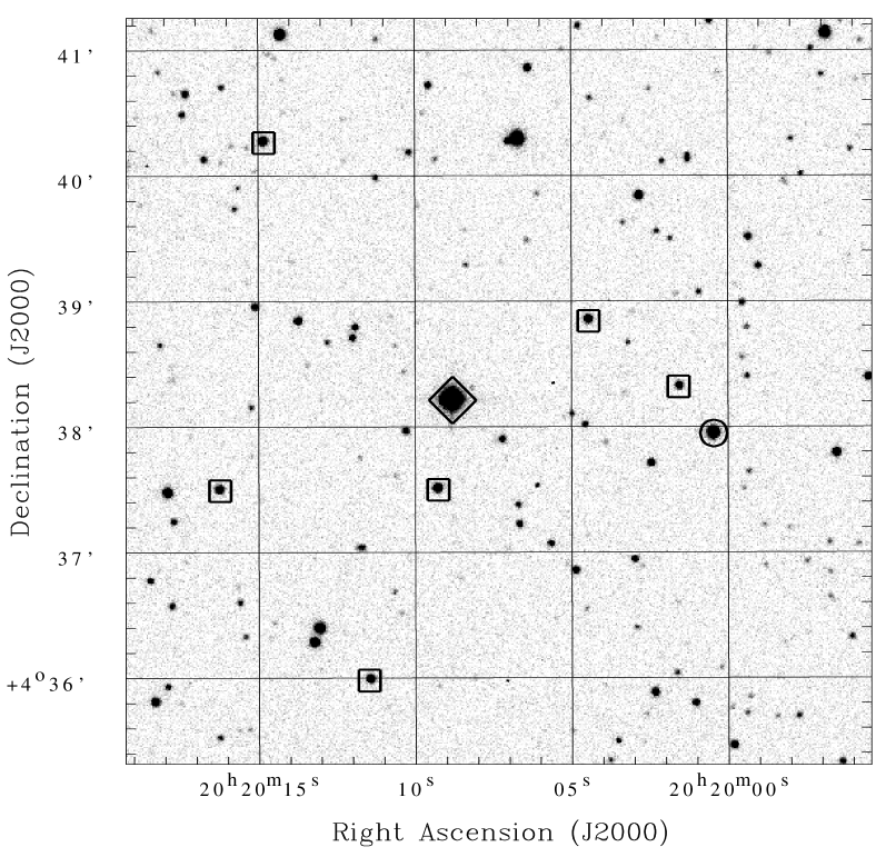
Figure 1: Finding chart for NSVS 14256825 in the R_C band obtained using the OPD/LNA 0.6-m telescope. The circle shows NSVS 1425, the diamond is the adopted reference star, and the squares outline additional comparison stars.

Figure 2: Calibrated NSVS 1425 light curves in the U, B, V, R_C, I_C, J, and H bands folded on the 0.1104 d orbital period. The R_C-band curve was displaced upwards by 0.5 mag to improve visualisation.

Table 2: Log of the photometric observations.

UT Date	$N$	texp(s)	Telescope	Filter
2010 Jul 30	300	20	0.6-m	RC
2010 Jul 30	185	30	1.6-m	J
2010 Jul 31	250	30	0.6-m	B
2010 Jul 31	450	20	0.6-m	RC
2010 Jul 31	177	30	1.6-m	J
2010 Jul 31	235	30	1.6-m	H
2010 Aug 01	235	40	0.6-m	U
2010 Aug 01	75	40	0.6-m	B
2010 Aug 01	100	30	1.6-m	Y
2010 Aug 01	215	30	1.6-m	J
2010 Aug 02	230	40	0.6-m	U
2010 Aug 02	400	20	0.6-m	IC
2010 Aug 06	120	30	0.6-m	V
2010 Aug 07	220	30	0.6-m	V
2010 Aug 08	220	30	0.6-m	IC
2010 Aug 09	160	25	0.6-m	RC
2010 Aug 10	80	25	0.6-m	RC
2010 Aug 18	800	10	0.6-m	RC
2010 Aug 18	530	15	0.6-m	IC
2010 Aug 19	225	40	0.6-m	U
2010 Aug 20	420	20	0.6-m	B
2010 Sep 01	160	30	0.6-m	V
2010 Sep 03	250	30	1.6-m	J
2010 Sep 04	142	50	1.6-m	J
2010 Nov 03	352	20	0.6-m	IC

2.2 Optical spectroscopy

The spectroscopic observations were performed using the Cassegrain spectrograph attached to the 1.6-m telescope at OPD/LNA. Thirty six (36) spectra were obtained using the 1200 l/mm grating and integration times of 10 or 15 minutes. The spectral coverage of this configuration is 3950-4900 Å, using 1.8 Å resolution (from the FWHM of the wavelength calibration lines). A hundred (100) bias frames and 30 flat-field frames were obtained each night to remove systematic signatures from the CCD detector. Observations of a He-Ar comparison lamp were made every two exposures on the target to provide wavelength calibration. The spectrophotometric standard stars HR 1544, HR 7596, and HR 9087 (Hamuy et al., 1992) were observed for flux calibration.

The reduction of the spectra was carried out following the steps of bias subtraction, flat-field structure removal, optimal extraction, wavelength calibration, and flux calibration using the standard routines in IRAF. The upper panel in Figure 3 shows a typical normalised individual spectrum. The lower panel shows the average of all spectra after Doppler shifting using the radial velocity orbital solution (see Section 3.2).

Figure 3: Upper panel: a normalised individual spectrum of NSVS 1425 with 900 s integration time. Lower panel: the average of 36 spectra after correcting for orbital motion.

3 Analysis and Results

Table 3: Apparent magnitudes of NSVS 1425 at primary and secondary minima.

UT Date	Band	Primary	Secondary
		minimum	minimum
2010 Aug 02	U	12.41$\pm$0.20	11.73$\pm$0.20
2010 Aug 20	B	13.76$\pm$0.15	13.06$\pm$0.15
2010 Aug 07	V	13.93$\pm$0.13	13.23$\pm$0.13
2010 Jul 31	RC	13.79$\pm$0.12	13.10$\pm$0.12
2010 Aug 18	IC	14.18$\pm$0.16	13.47$\pm$0.16
2010 Aug 01	J	14.50$\pm$0.24	13.80$\pm$0.24
2010 Jul 31	H	14.60$\pm$0.25	13.91$\pm$0.25

3.1 Ephemeris

To determine an ephemeris for the times of the primary minimum in NSVS 1425, we combined our timings and those from Wils et al. (2007), after converting them to barycentric dynamical time (TDB). Our eclipse timings were obtained by modelling the primary eclipse using the Wilson-Devinney (WD) code (Wilson & Devinney, 1971) together with a Markov chain Monte Carlo (MCMC) procedure (Gilks, Richardson & Spiegelhalter, 1996) to obtain the uncertainties. The geometrical and physical parameters of the system are calculated as described in Section 3.4. These parameters were used as fixed inputs for the WD code and only the times of individual primary eclipses are left as free parameters. The median values and the 1-$\sigma$ uncertainties obtained from the marginal distribution of the fitted instants of minimum were adopted as the best values for location and error of each timing. Using the expression $T_{\rm min}=T_{0}+E\times P$, where $T_{\rm min}$ are the predicted times of primary minimum, $T_{0}$ is a fiducial epoch, $E$ is the cycle count from $T_{0}$, and $P$ is the binary orbital period, we obtained the following ephemeris,

$$T_{\rm min}={\rm TDB}\,2454274.2087(1)+0.110374230(2)\times E.$$ (1)

3.2 Radial velocity solution

The radial velocities were obtained using the task FXCOR in IRAF. Initially, a combination of all 36 spectra was used as a template for the cross correlation with the individual spectra. Regions around H$\beta$, H$\gamma$, H$\delta$, H$\epsilon$, and HeII $\lambda$4686 were selected (see Figure 3) to improve the signal/noise ratio of the correlation procedure. The resulting radial velocity solution was used to Doppler shift all individual spectra to the orbital rest frame. A better quality template is then produced from these rest-frame spectra. The procedure was iterated a number of times until the radial velocity solution converged. Table 4 lists individual radial velocities and Figure 4 shows the radial velocity curve folded on the orbital phase together with the best solution for a circular orbit. The modelling provides a semi-amplitude $K_{1}=73.4\pm 2.0$ km s^-1 and a systemic velocity $\gamma=-12.1\pm 1.5$ km s^-1.

Figure 4: Radial velocity of the prominent lines in the spectra of NSVS 1425. The phases are calculated using the ephemeris presented in Section 3.1.

Table 4: Spectroscopic observations and radial velocities.

UT Date	BJD(TDB)	texp	V	Orbital
	(2450000+)	(s)	(km s-1)	Phase
2010 Set 01	5441.48256	900	2.29$\pm$12.29	0.60
2010 Set 01	5441.49251	600	-8.05$\pm$11.86	0.69
2010 Set 01	5441.50371	900	66.46$\pm$10.50	0.79
2010 Set 01	5441.51799	900	12.46$\pm$10.60	0.92
2010 Set 01	5441.52904	900	-40.38$\pm$12.10	0.02
2010 Set 01	5441.54078	900	-67.43$\pm$10.21	0.13
2010 Set 01	5441.55825	900	-83.52$\pm$11.16	0.29
2010 Set 01	5441.56970	900	-64.55$\pm$10.12	0.39
2010 Set 01	5441.58084	900	-21.99$\pm$12.32	0.49
2010 Set 01	5441.59792	900	53.03$\pm$12.84	0.65
2010 Set 01	5441.60920	900	60.29$\pm$10.98	0.75
2010 Set 01	5441.62057	900	47.18$\pm$9.33	0.85
2010 Set 01	5441.63857	900	-44.83$\pm$10.33	0.02
2010 Set 01	5441.65259	900	-78.09$\pm$12.25	0.14
2010 Set 01	5441.66364	900	-76.39$\pm$12.18	0.24
2010 Set 02	5442.42478	900	-63.45$\pm$10.09	0.14
2010 Set 02	5442.43581	900	-84.04$\pm$10.91	0.24
2010 Set 02	5442.45306	900	-37.19$\pm$9.84	0.40
2010 Set 02	5442.46413	900	-6.20$\pm$8.10	0.50
2010 Set 02	5442.48116	900	44.56$\pm$8.03	0.65
2010 Set 02	5442.49223	900	65.25$\pm$9.62	0.75
2010 Set 02	5442.51304	900	32.99$\pm$10.88	0.94
2010 Set 02	5442.52404	900	-32.57$\pm$8.55	0.04
2010 Set 02	5442.54110	900	-82.53$\pm$7.39	0.19
2010 Set 02	5442.55209	900	-77.39$\pm$8.10	0.29
2010 Set 02	5442.56870	900	-30.80$\pm$10.13	0.44
2010 Set 02	5442.57970	900	20.41$\pm$10.04	0.54
2010 Set 02	5442.60086	900	57.22$\pm$11.46	0.74
2010 Set 02	5442.61186	900	58.08$\pm$9.66	0.83
2010 Set 02	5442.62893	900	-8.53$\pm$10.40	0.98
2010 Set 02	5442.63992	900	-65.09$\pm$9.83	0.09
2010 Set 02	5442.65664	900	-91.21$\pm$10.98	0.24
2010 Set 02	5442.66763	900	-70.64$\pm$11.55	0.34
2010 Set 02	5442.68442	900	-3.21$\pm$6.66	0.49
2010 Set 02	5442.69542	900	23.22$\pm$10.57	0.59
2010 Set 02	5442.71246	900	47.40$\pm$9.12	0.74

3.3 Atmospheric parameters

The atmospheric parameters of the sdB star can be determined using the Balmer and helium lines in the blue range of the spectrum. The spectra obtained in a 0.1 phase interval centred in the secondary eclipse, i.e., 0.45–0.55, were used to minimise the contribution of the reflection effect. Using $\chi^{2}$ as the figure of merit, the combined spectrum was matched to a grid of synthetic spectra retrieved from the web page of TheoSSA. The synthetic spectra were calculated by the Tübingen non-local thermodynamic equilibrium Model-Atmosphere Package (TMAP). Two different metallicities were used: Model A with zero metallicity; and Model B with the metallicity adopted by Klepp & Rauch (2011). The grid is composed by: 26 values of effective temperatures, 30000 K $\leq$ T $\leq$ 43000 K with 500 K steps; 16 surface gravities, $5.2\leq\log g\leq 6.0$ with 0.05 dex steps; and 10 helium abundances, 0.001 $\leq$ $n(\rm He)$/$n(\rm H)$ $\leq$ 0.01 with 0.001 dex steps. All synthetic spectra were convolved with the projected rotational velocity $v\sin\,i=73.4$ km s^-1 and with an instrumental profile of FWHM 1.8 Å.

The synthetic Balmer (H$\beta$ to H$\epsilon$) and helium (HeI $\lambda 4471$ and HeII ${\lambda 4686}$) lines were used in the fitting procedure to determine the effective temperature, surface gravity, and He abundance. The best fit yields $T=38000\pm 500$ K, $\log g=5.2\pm 0.05$, and $n(\rm He)$/$n(\rm H)=0.003\pm 0.001$ for the Model A, and $T=40000\pm 500$ K, $\log g=5.50\pm 0.05$, and $n(\rm He)$/$n(\rm H)=0.003\pm 0.001$ for Model B. Figure 5 shows the observed spectra together with the best synthetic spectra for both models. The $\chi^{2}$ of model B is $\sim$5 per cent better than that of model A.

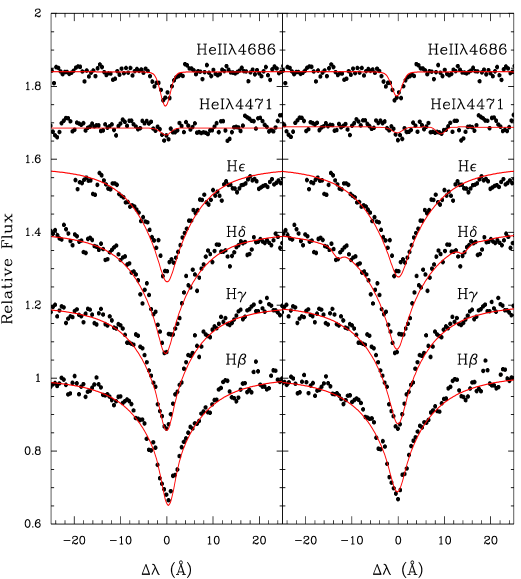
Figure 5: The best fits to the Balmer and helium lines used to derive effective temperature, surface gravity, and helium abundance. The observed spectra are presented using black dots and the red lines represent the best-fit synthetic spectra. The left and right panels correspond to models with zero metallicity and the metallicity from Klepp & Rauch (2011), respectively.

3.4 Simultaneous modelling of light curves and radial velocities

In order to obtain the geometrical and physical parameters for NSVS 1425, we simultaneously analysed the U, B, V, R_C, I_C, J, and H light curves and the radial velocity curve using the WD code. The original WD code uses a differential correction method for improving an initial solution. This method works well if the initial parameter values are close to those corresponding to the optimal solution. However, if they are close to a local minimum, the differential correction procedure may fail to find the best solution. To solve this problem, the WD code was used as a “function” to be optimised by the genetic algorithm PIKAIA (Charbonneau, 1995), which is adequate to search for a global minimum in a model involving a large set of parameters.

To examine the marginal distribution of probability of the parameters and to establish realistic uncertainties, we used the solution obtained by PIKAIA as an input to an MCMC procedure.

Due to the large number of parameters to be fitted, it is important to constrain them using theoretical and spectroscopic information. From the spectroscopic analysis, we adopted the effective temperature of the primary star as an initial value. We can also constrain the mass ratio, $q$, using the mass function (Eq. 2) and assuming that the mass of the sdB star, $M_{1}$, is in the range $0.1-0.8~{}\rm M_{\odot}$ (Driebe et al., 1998; Han et al., 2003), and that the radial velocity semi-amplitude, $K_{1}$, is 73.4 km s^-1.

$$\frac{M_{1}\times(q\sin\,i)^{3}}{(1+q)^{2}}=1.0361\times 10^{-7}(1-e^{2})^{3/2}K_{1}^{3}P.$$ (2)

As the components are in close orbit, the timescales of synchronisation and circularisation are much shorter than the helium burning lifetime (Zahn, 1977). Thus, the orbit can be considered circular ($e$ = 0) and the rotation of the components synchronised with the orbit. Finally, adopting the range of orbital inclinations for eclipsing binaries, $75^{\circ}<i<90^{\circ}$, we obtained $0.21<q<0.45$ for the mass ratio range.

Mode 2 of the WD code, which sets no constraints on the Roche configuration, was used. The luminosity of the secondary star was computed assuming stellar atmosphere radiation. Linear limb darkening coefficients, $x_{i}$, were used for both stars. Regarding the sdB star, we used the coefficients calculated by Díaz-Cordovés, Claret & Gimenez (1995) and Claret, Díaz-Cordovés & Gimenez (1995) for a star with effective temperature $T=40000$ K and surface gravity $\log g=5.0$. These are the closest values to those of the hot component in NSVS 1425 for which limb darkening coefficients have been published in literature. On the other hand, the linear limb darkening coefficients of the cool star were left as free parameters, since the proximity of the hot star can significantly change these coefficients with respect to those of a single star. As the sdB star has a radiative envelope, its gravity darkening exponent, $\beta_{1}$, and its bolometric albedo for reflective heating and re-radiation, $A_{1}$, were set to unity (Rafert & Twigg, 1980). The gravity darkening exponent of the secondary component, $\beta_{2}$, was fixed at 0.3, which is appropriate for convective stars (Lucy, 1967). As shown by For et al. (2010), Kilkenny et al. (1998), and Drechsel et al. (2001), the albedo of the secondary star, $A_{2}$, can assume physically unrealistic values $A_{2}>1$, especially at longer wavelengths where the reflected-reradiated light is more intense. For this reason, it was decided to perform two modellings: in Model 1, we adopt a constant (but free parameter) secondary albedo for all photometric bands; in Model 2, we consider variable and independent albedos for all photometric bands.

In both cases the remaining fitted parameters consist of: the mass ratio, $q=M_{2}/M_{1}$; the orbital inclination, $i$; the separation between the components, $a$; the Roche potentials, $\Omega_{1}$ and $\Omega_{2}$; and the effective temperatures of the two stars, $T_{1}$ and $T_{2}$.

In order to optimise the computational time, all light curves were binned with 160 seconds time resolution and the error of the bin average outside of the eclipses was assumed as the uncertainty. To test the goodness of fit, we use the reduced $\chi^{2}$ defined as

$$\centering\chi^{2}=\frac{1}{n}\sum_{i}^{n}\left(\frac{O_{i}-C_{i}}{\sigma_{i}}\right)^{2},\@add@centering$$ (3)

where $O_{i}$ are the observed points, $C_{i}$ are the corresponding model, $\sigma_{i}$ are the uncertainties at each point, and $n$ is the number of points. Figure 6 shows the best fit together with the light and radial velocity curves while Table 5 lists the fitted and fixed parameters.

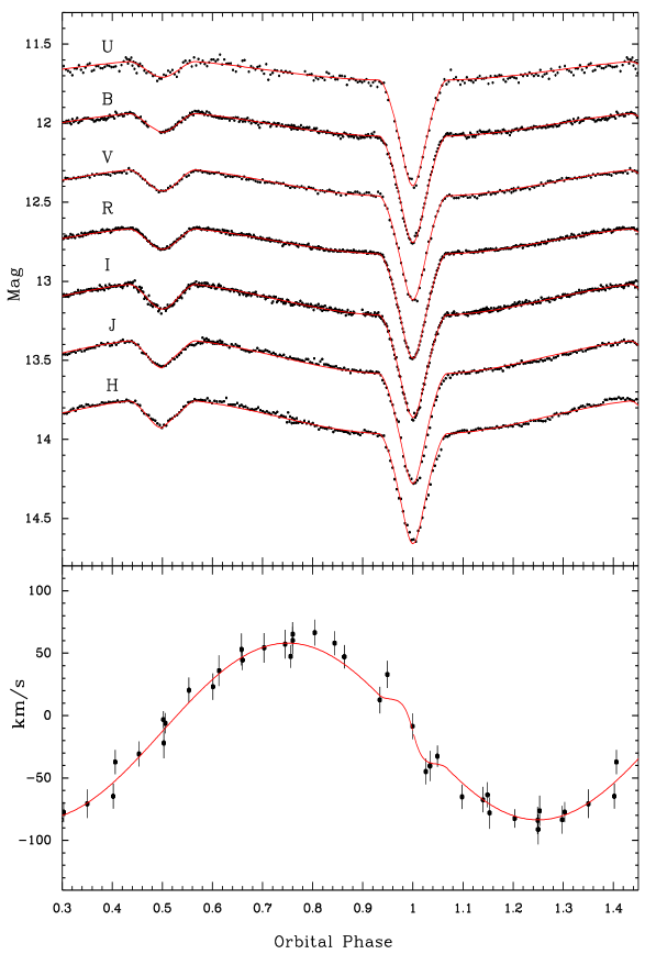
Figure 6: The best simultaneous fit for the U, B, V, R_C, I_C, J, H light curves and radial velocity data using the WD code. The light curves are the same as those shown in Figure 2 displaced vertically for better visualisation.

Table 5: System parameters of the best fit for photometric light curves in U, B, V, R_C, I_C, J and H bands and radial velocity data for NSVS 1425.

Parameter	Model 1	Model 2
Fitted Parameters
$q=(M_{2}/M_{1})$	$0.28\pm 0.013$	$0.26\pm 0.012$
$i~{}(^{\circ}$)	$82.5\pm 0.4$	$82.5\pm 0.3$
$\Omega^{a}_{1}$	$4.58\pm 0.13$	$4.55\pm 0.11$
$\Omega^{a}_{2}$	$2.80\pm 0.15$	$2.69\pm 0.12$
$T_{1}$(K)	$42300\pm 400$	$42000\pm 500$
$T_{2}$(K)	$2400\pm 600$	$2550\pm 550$
$a^{b}$ (R⊙)	$0.74\pm 0.04$	$0.80\pm 0.04$
$A^{c}_{2}$(U)	$1.50\pm 0.11$	$2.0\pm 0.15$
$A^{c}_{2}$(B)	$1.50\pm 0.11$	$1.35\pm 0.13$
$A^{c}_{2}$(V)	$1.50\pm 0.11$	$1.20\pm 0.12$
$A^{c}_{2}$(RC)	$1.50\pm 0.11$	$1.05\pm 0.09$
$A^{c}_{2}$(IC)	$1.50\pm 0.11$	$1.3\pm 0.12$
$A^{c}_{2}$(J)	$1.50\pm 0.11$	$0.95\pm 0.14$
$A^{c}_{2}$(H)	$1.50\pm 0.11$	$1.10\pm 0.15$
$x_{2}$(U)	$0.64\pm 0.04$	$0.68\pm 0.04$
$x_{2}$(B)	$0.69\pm 0.04$	$0.74\pm 0.05$
$x_{2}$(V)	$0.78\pm 0.03$	$0.80\pm 0.04$
$x_{2}$(RC)	$0.83\pm 0.02$	$0.87\pm 0.02$
$x_{2}$(IC)	$0.90\pm 0.03$	$0.92\pm 0.03$
$x_{2}$(J)	$0.93\pm 0.04$	$0.95\pm 0.04$
$x_{2}$(H)	$0.98\pm 0.05$	$0.99\pm 0.05$
Roche radiih
$r_{1}$ (pole)	0.231$\pm$0.006	0.233$\pm$0.005
$r_{1}$ (side)	0.233$\pm$0.006	0.235$\pm$0.005
$r_{1}$ (point)	0.235$\pm$0.007	0.236$\pm$0.006
$r_{1}$ (back)	0.234$\pm$0.007	0.236$\pm$0.006
$r_{2}$ (pole)	0.180$\pm$0.016	0.194$\pm$0.014
$r_{2}$ (side)	0.182$\pm$0.016	0.198$\pm$0.016
$r_{2}$ (point)	0.191$\pm$0.019	0.210$\pm$0.019
$r_{2}$ (back)	0.189$\pm$0.019	0.207$\pm$0.018
Fixed Parameters
$A^{c}_{1}$	1.0	1.0
$\beta^{d}_{1}$	1.0	1.0
$\beta^{d}_{2}$	0.3	0.3
$x^{e}_{1}$(U)	0.242	0.242
$x^{e}_{1}$(B)	0.233	0.233
$x^{e}_{1}$(V)	0.209	0.209
$x^{f}_{1}$(RC)	0.176	0.176
$x^{f}_{1}$(IC)	0.147	0.147
$x^{f}_{1}$(J)	0.112	0.112
$x^{f}_{1}$(H)	0.095	0.095
Goodness of fit
$\chi^{2}$	2.1	1.2

^a Roche surface potential;
^b Components separation;
^c Bolometric albedo;
^d Gravity darkening exponent;
^e Linear limb darkening coefficient from Díaz-Cordovés et al. (1995);
^f Linear limb darkening coefficient from Claret et al. (1995);
^h In units of orbital separation.

The values found for almost all parameters in the two models are consistent. However, the $\chi^{2}$ for Model 2 is $\sim$40 per cent better than for Model 1.

3.5 Fundamental Parameters

Physical and geometrical parameters such as masses, radii, and separation between the two components of the system can be derived from the solutions obtained in the previous sections. Substituting the values of the orbital period ($P_{\rm orb}=0.110374230$ d), semi-amplitude of the radial velocity ($K_{1}=73.4$ km s^-1), mass ratio ($q=0.260$), and inclination ($i=82\aas@@fstack{\circ}5$) in Eq. 2, $M_{1}=0.419\pm 0.070~{}\rm M_{\odot}$ is obtained for the primary mass. The primary mass and the mass ratio are used to derive the secondary mass, $M_{2}=0.109\pm 0.023~{}\rm M_{\odot}$. Using Kepler’s Third Law, one can obtain the orbital separation, $a=0.80\pm 0.04~{}\rm R_{\odot}$, from which the absolute radii follow, $R_{1}=0.188\pm 0.010~{}\rm R_{\odot}$ and $R_{2}=0.162\pm 0.008~{}\rm R_{\odot}$. In Table 6 we show the fundamental parameters for NSVS 1425 derived from Model 1 and Model 2.

Table 6: Fundamental parameters for NSVS 1425.

Parameter	Model 1	Model 2
$M_{1}$ (M⊙)	0.346$\pm$0.079	0.419$\pm$0.070
$M_{2}$ (M⊙)	0.097$\pm$0.028	0.109$\pm$0.023
$R_{1}$ (R⊙)	0.173$\pm$0.010	0.188$\pm$0.010
$R_{2}$ (R⊙)	0.137$\pm$0.008	0.162$\pm$0.008
$T_{1}$ (K)	42300$\pm$500	42000$\pm$400
$T_{2}$ (K)	2400$\pm$500	2550$\pm$500
$\log g_{1}$	5.50$\pm$0.14	5.51$\pm$0.11
$\log g_{2}$	5.15$\pm$0.16	5.05$\pm$0.13
$a$ (R⊙)	0.74$\pm$0.04	0.80$\pm$0.04

3.6 Rossiter-McLaughlin effect

An interesting spectroscopic signature in eclipsing binary systems is the Rossiter-McLaughlin (RM) effect (Rossiter, 1924; McLaughlin, 1924). This effect occurs when the eclipsed object rotates. There is evidence of this effect on the radial velocity curve in the phase interval $0.95-1.05$ (Figure 6). Unfortunately, our data are not enough to model the RM effect to derive the alignment rotational parameters of the NSVS 1425 stars. However, our observed points are consistent with the predicted RM effect for aligned rotating stars obtained by the WD code with the parameters shown in Table 5.

4 Discussion

4.1 Characteristics of the primary star

Of all HW Vir systems, the primary of NSVS 1425 has the second highest temperature (see Table 1), consistent with the prominent HeII $\lambda$4686 line (see Figure 3). Accordingly, we suggest that the primary of NSVS 1425 is an sdBO star which means this system is very similar to AA Dor and, hence, in a rare evolutionary stage (Heber, 2009).

Comparing the values of $\log g$ derived from the simultaneous fit to photometric and spectroscopic data (Table 6) with those obtained from the modelling of the spectral lines of the primary star (Section 3.3), it is clear that the model with metallicity equal to that adopted by Klepp & Rauch (2011) provides consistent results, whereas the model with zero metallicity has a discrepancy. We noticed that the same kind of discrepancy had been found by Rauch (2000) in the analysis of the primary in AA Dor. Rauch (2000) obtained $\log g=5.21$ from spectroscopic data, whereas Hilditch, Harries, & Hill (1996) had derived $\log g=5.53$ from photometric data modelling. This discrepancy was solved by Klepp & Rauch (2011) with the improvement of the Stark broadening modelling, the minimisation of the reflection effect, and adoption of metal-line blanketing.

4.2 Evolution

Han et al. (2003), from a detailed binary population synthesis study, presented three possible channels for forming sdB stars:

1. One or two phases of common envelope (CE) evolution;

2. One or two stable Roche lobe overflows;

3. A merger of two He-core white dwarfs.

Driebe et al. (1998) and Heber et al. (2003) suggest another scenario to form an sdB star with low mass in binaries called post-RGB. This scenario is similar to the channel (i) proposed by Han et al. (2003), except that the resultant sdB in the first CE phase has insufficient mass in its core to ignite helium. However, it will evolve as a helium star through the sdB star region to form a helium core white dwarf.

In Figure 7 we compare the position of the primary component of NSVS 1425 on the ($T_{\rm eff}$, $\log g$) diagram with other sdB stars in short-period binary systems (see Table 1). We also show a sample of single sdB and sdOB stars analysed by Edelmann (2003). In the same graph we display evolutionary tracks for different masses in the post-EHB calculated by Dorman, Rood & O’Connell (1993) for single star evolution. As can be seen, the position of the NSVS 1425 primary is close to that of the AA Dor primary. The evolutionary track for single star evolution would only marginally explain the mass obtained for the sdB star in NSVS 1425. Out of the possible channels to form an sdB in binaries, we suggest that the channel (i) is probably the evolutionary scenario for NSVS 1425.

Figure 7: Position on the ($T_{\rm eff}$, $\log g$) diagram of the hot component of NSVS 1425 compared with other sdB stars (see Table 1). Isolated sdB and sdOB stars presented in Edelmann (2003) are shown with open circles. Dashed lines represent evolutionary tracks for different masses in the post-EHB evolution (Dorman et al., 1993). The zero age extreme horizontal branch (ZAEHB) and terminal age extreme horizontal branch (TAEHB) are represented by solid lines.

5 Conclusion

We present a photometric and spectroscopic analysis of the NSVS 1425 system. With a short orbital period, $P=0.110374230(2)$ d, this binary shows both primary and secondary eclipses and a prominent reflection effect. From the spectroscopic analysis we obtain $73.4\pm 2.0~{}\rm km~{}s^{-1}$ for the semi-amplitude of the radial velocity and $-12.1\pm 1.5~{}\rm km~{}s^{-1}$ for the systemic velocity. The atmospheric parameters of the primary component (sdOB star), namely, effective temperature, $T=40000\pm 500$ K, surface gravity, $\log g=5.5\pm 0.05$, and Helium abundance, $n(\rm He)$/$n(\rm H)=0.003\pm 0.001$, were calculated matching the observed spectrum to a grid of NLTE synthetic spectra.

Simultaneously fitting the U, B, V, R_C, I_C, J, and H-bands light curves and radial velocity curve using the WD code, the geometrical and physical parameters of NSVS 1425 were obtained. These results allow us to derive the absolute parameters of the system such as masses and radii of the components.

We compare the position of the sdB star in NSVS 1425 with other sdB and sdOB stars on the effective temperature versus surface gravity diagram. We describe the possible channels to form an sdB star in binaries and conclude that the post-common envelope development is probably the evolutionary scenario for NSVS 1425. The subsequent evolution of this system should lead to a cataclysmic variable. After a phase of angular momentum loss via gravitational radiation, this system will lie below the period gap of the cataclysmic variables.

References

- Charbonneau (1995) Charbonneau P., 1995, ApJS, 101, 309
- Charpinet et al. (2008) Charpinet S., van Grootel V., Reese D., Fontaine G., Green E. M., Brassard P., Chayer P., 2008, A&A, 489, 377
- Claret et al. (1995) Claret A., Díaz-Cordovés J., Gimenez A., 1995, A&AS, 114, 247
- Díaz-Cordovés et al. (1995) Díaz-Cordovés J., Claret A., Gimenez A., 1995, A&AS, 110, 329
- Dorman et al. (1993) Dorman B., Rood R. T., O’Connell R. W., 1993, ApJ, 419, 596
- Drechsel et al. (2001) Drechsel H. et al., 2001, A&A, 379, 893
- Driebe et al. (1998) Driebe T., Schönberner D., Blöker T., Herwig F., 1998, A&A, 339, 123
- For et al. (2010) For B. -Q. et al., 2010, ApJ, 708, 253
- Edelmann (2003) Edelmann H., 2003, A&A, 400, 939
- Geier et al. (2011) Geier S. et al., 2011, ApJL, 731, L22
- Gilks, Richardson & Spiegelhalter (1996) Gilks W. R., Richardson S., Spiegelhalter D. J. E., 1996, Markov Chain Monte Carlo in Practice, Chapman & Hall, London
- Kilkenny et al. (1998) Kilkenny D., O’Donoghue D., Koen C., Lynas-Gray A. E., van Wyk F., 1998, MNRAS, 296, 329
- Hamuy et al. (1992) Hamuy M., Walker A. R., Suntzeff N. B., Gigoux P., Heathcote S. R., Phillips M. M., 1992, PASP, 104, 533
- Han et al. (2003) Han Z., Podsiadlowski P., Maxted P. F. L., Marsh T. R., 2003, MNRAS, 341, 669
- Heber (2009) Heber U., 2009, ARA&A, 47, 211
- Heber et al. (2003) Heber U. et al., 2003, A&A, 411, L477
- Hilditch, Harries, & Hill (1996) Hilditch R. W., Harries T. J., Hill G., 1996, MNRAS, 279, 1380
- Hilditch et al. (2003) Hilditch R. W., Kilkenny D., Lynas-Gray A. E., Hill G., 2003, MNRAS, 344, 644
- Klepp & Rauch (2011) Klepp S., Rauch T., 2011, A&A, 531, L7
- Lucy (1967) Lucy L. B., 1967, Z. Astrophysics, 65, 89
- McLaughlin (1924) McLaughlin D. B., 1924, AJ, 60, 22
- Østensen et al. (2007) Østensen R., Oreiro R., Drechsel H., Heber U., Baran A., Pigulski A., 2007, ASPC, 372, 483
- Østensen et al. (2010) Østensen R. H. et al., 2010, MNRAS, 408, L51
- Polubek et al. (2007) Polubek G., Pigulski A., Baran A., Udalski A., 2007, ASPC, 372, 487
- Rafert & Twigg (1980) Rafert J. B., Twigg L. W., 1980, MNRAS, 193, 79
- Rauch (2000) Rauch T., 2000, A&A, 356, 665
- Rossiter (1924) Rossiter R. A., 1924, ApJ, 60, 15
- Rucinski (2009) Rucinski S. M., 2009, MNRAS, 395, 2299
- Taam & Ricker (2010) Taam R. E., Ricker P. L., 2010, NewAR, 54, 65
- Tody (1993) Tody D., 1993, ASPC, 52, 173
- Vuĉković et al. (2009) Vuĉković M. et al., 2008, A&A, 505, 239
- Wils et al. (2007) Wils P., Giorgio D., Sebastián A. O., 2007, IBVS, 5800
- Wilson & Devinney (1971) Wilson R. E., Devinney E. J., 1971, ApJ, 166, 605
- Wood & Saffer (1999) Wood J. H., & Saffer R., 1999, MNRAS, 305, 820
- Wozniak et al. (2004) Woźniak P. R., Williams S. J., Vestrand W. T., Gupta V., 2004, AJ, 128, 2965
- Zahn (1977) Zahn J. -P., 1977, A&A, 57, 383