Active region formation through the negative effective magnetic pressure instability

Abstract

The negative effective magnetic pressure instability operates on scales encompassing many turbulent eddies and is here discussed in connection with the formation of active regions near the surface layers of the Sun. This instability is related to the negative contribution of turbulence to the mean magnetic pressure that causes the formation of large-scale magnetic structures. For an isothermal layer, direct numerical simulations and mean-field simulations of this phenomenon are shown to agree in many details in that their onset occurs at the same depth. This depth increases with increasing field strength, such that the maximum growth rate of this instability is independent of the field strength, provided the magnetic structures are fully contained within the domain. A linear stability analysis is shown to support this finding. The instability also leads to a redistribution of turbulent intensity and gas pressure that could provide direct observational signatures.

1 Introduction

Active region formation in the Sun is traditionally thought to be a deeply rooted phenomenon, because their size ($\sim 100\,{\rm Mm}$) is much larger than the naturally occurring scales in the surface layers of the convection zone ($\sim 1$–$10\,{\rm Mm}$); see Golub et al. (1981). They are also long-lived ($\sim 1/2$ year), which seems unnaturally long if associated with the near-surface layers ($40\,{\rm Mm}$ depth) where typical time scales are about a day. On the other hand, a deeply rooted formation scenario for active regions has the problem that the azimuthal pattern speed of active regions does not match the angular velocity at great depth. Other difficulties concern the strong field strength inferred for the tachocline to explain the observed tilt angles and the fact that magnetic structures expand tremendously during their ascent. These and several other arguments have led to the consideration of solar activity as a shallow phenomenon; see Brandenburg (2005) for details. As a possible mechanism for producing magnetic flux concentrations of the form of active regions, the negative effective magnetic pressure instability has been discussed (Kleeorin et al., 1989, 1990; Kleeorin & Rogachevskii, 1994; Kleeorin, Mond, and Rogachevskii, 1996; Rogachevskii & Kleeorin, 2007; Brandenburg et al., 2010, 2011). Of course a magnetic field $B$ always gives rise to a positive magnetic pressure, $\mbox{\boldmath$B$}{}^{2}/2\mu_{0}$, where $\mu_{0}$ is the vacuum permeability. In a turbulent medium, however, magnetic fields also suppress the turbulence and thus decrease the turbulent pressure $\rho\mbox{\boldmath$u$}{}^{2}/3$, and modify the pressure caused by magnetic fluctuations $\bm{b}^{2}/6\mu_{0}$. Here, $u$ and $\bm{b}$ are velocity and magnetic fluctuations, $\rho$ is the density, $\mu_{0}$ is the vacuum permeability, and the coefficients in the turbulent fluid and magnetic pressure are given for isotropic turbulence. Magnetic fluctuations can be due to both small-scale dynamo action as well as tangling of a large-scale field, $\overline{\mbox{\boldmath$B$}}{}$. The total field is thus $\mbox{\boldmath$B$}{}=\overline{\mbox{\boldmath$B$}}{}+\bm{b}$. The sum of both effects, $p_{\rm turb}=\overline{\rho\mbox{\boldmath$u$}{}^{2}}/3+\langle\bm{b}^{2}\rangle/6\mu_{0}$, is positive definite, but it depends on $\overline{\mbox{\boldmath$B$}}{}$, and $p_{\rm turb}$ tends to decline as $\overline{B}\equiv|\overline{\mbox{\boldmath$B$}}{}|$ increases. Indeed, $p_{\rm turb}=2E_{K}/3-\langle\bm{b}^{2}\rangle/6\mu_{0}$, where $E_{K}=\overline{\rho\mbox{\boldmath$u$}{}^{2}}/2+\langle\bm{b}^{2}\rangle/2\mu_{0}\approx$ const, so that the change of the turbulent pressure is negative $(\delta p_{\rm turb}<0)$ when the magnetic fluctuations are generated by tangling of the mean magnetic field by the velocity fluctuations at the expanse of turbulent kinetic energy (Kleeorin et al., 1990; Brandenburg et al., 2011). Thus, we write

$$p_{\rm turb}(\overline{B})=p_{\rm turb}(0)-q_{\rm p}(\overline{B})\overline{B}^{2}/2\mu_{0},$$ (1)

where $p_{\rm turb}(0)$ is the turbulent pressure at zero mean field. The pressure $p_{\rm turb}(0)$ only includes those contributions from $\bm{b}^{2}$ that are associated with small-scale dynamo action, but not those resulting from the mean field. The relevant magnetic pressure in the evolution equation for the mean flow, $\overline{\bm{U}}$, is then not just $\overline{B}^{2}/2\mu_{0}$, but it is affected by the $\overline{B}$ dependence of $p_{\rm turb}$, i.e., it depends on

$$p_{\rm turb}(\overline{B})+\overline{B}^{2}/2\mu_{0}=p_{\rm turb}(0)+[1-q_{\rm p}(\overline{B})]\overline{B}^{2}/2\mu_{0},$$ (2)

which is also still positive, but $1-q_{\rm p}(\overline{B})$ may well become negative, which is what we call a negative effective magnetic pressure. Consequently, the expression

$$p_{\rm eff}=(1-q_{\rm p})\overline{\mbox{\boldmath$B$}}{}^{2}/2\mu_{0}$$ (3)

is referred to as the effective magnetic pressure. In addition, there is also the gas pressure $p_{\rm gas}$. Once the effective magnetic pressure drives a mean flow, the gas density changes, and as a consequence the gas pressure, so as to re-establish approximate total pressure balance. Therefore, $p_{\rm gas}$ and $\rho$ will also depend on $\overline{B}$.

In the presence of gravity, the properties of magnetic buoyancy are drastically altered by a negative effective magnetic pressure. In the following we illustrate how this can lead to an instability. Since the flow velocities are highly subsonic, we can make the anelastic approximation for low Mach numbers, i.e., $\mbox{\boldmath$\nabla$}{}\cdot\overline{\rho}\overline{\bm{U}}=0$. This leads to $\mbox{\boldmath$\nabla$}{}\cdot\overline{\bm{U}}+\overline{\bm{U}}\cdot\mbox{\boldmath$\nabla$}{}\ln\overline{\rho}=0$, or

$$\mbox{\boldmath$\nabla$}{}\cdot\overline{\bm{U}}={\overline{U}_{z}\over H_{\rho}},\ilabel{divu}$$ (4)

where we have used the density scale height $H_{\rho}$, so that $\mbox{\boldmath$\nabla$}{}\ln\overline{\rho}=(0,0,-1/H_{\rho})$. This equation shows that a downward motion $\overline{U}_{z}<0$ leads to a compression, $\mbox{\boldmath$\nabla$}{}\cdot\overline{\bm{U}}<0$. This enhances an applied field locally. We consider an applied equilibrium magnetic field of the form $(0,B_{0},0)$ and the mean field has only a $y$ component, i.e., $\overline{\mbox{\boldmath$B$}}{}=(0,\overline{B}_{y}(x,z),0)$, so we have

$${{\rm D}{}\overline{B}_{y}\over{\rm D}{}t}=-\overline{B}_{y}\mbox{\boldmath$\nabla$}{}\cdot\overline{\bm{U}},\ilabel{DByDt}$$ (5)

where ${\rm D}{}/{\rm D}{}t=\partial/\partial+\overline{\bm{U}}\cdot\mbox{\boldmath$\nabla$}{}$ is the advective derivative. Note that for a magnetic field with only a $y$ component, but $\partial/\partial y=0$, there is no stretching term, so there is no term of the form $\overline{\mbox{\boldmath$B$}}{}\cdot\mbox{\boldmath$\nabla$}{}\overline{\bm{U}}$. Using Equation (divu), and linearizing Equation (DByDt) around $\overline{\bm{U}}=\bm{0}$ and $\overline{\mbox{\boldmath$B$}}{}=\mbox{\boldmath$B$}{}_{0}$, we have

$${\partial\overline{B}_{1y}\over\partial t}=-B_{0}{\overline{U}_{1z}\over H_{\rho}},\ilabel{induct-eq}$$ (6)

where subscripts 1 denote linearized quantities. The vertical velocity perturbation $\overline{U}_{1z}$ is caused by magnetic buoyancy. Assuming total pressure equilibrium, $p_{\rm gas}+p_{\rm eff}={\rm const}{}$, we see that an increase in the effective magnetic pressure causes a decrease is the gas pressure, i.e., $\delta p_{\rm gas}=-\delta p_{\rm eff}$, just like in the regular magnetic buoyancy instability. Therefore, the Archimedian buoyancy force is

$$-{\delta\rho\over\rho}g=-{\delta p_{\rm gas}\over p_{\rm gas}}g={\delta p_{\rm eff}\over\rho c_{\rm s}^{2}}g={{\rm d}{}p_{\rm eff}\over{\rm d}{}\overline{B}^{2}}{\delta\overline{B}^{2}\over\rho c_{\rm s}^{2}}g,$$ (7)

where we have used $p_{\rm gas}=\rho c_{\rm s}^{2}$ for an isothermal gas. In the regular magnetic buoyancy instability, without turbulence effects, we have $2\mu_{0}{\rm d}{}p_{\rm eff}/{\rm d}{}{\overline{B}}{}^{2}=1$. In the domain where the negative effective magnetic pressure effect causes ${\rm d}{}p_{\rm eff}/{\rm d}{}{\overline{B}}{}^{2}$ to be negative, a magnetic field enhancement leads to a further reduction of the local pressure, which is compensated by horizontal inflows, increasing density (and field strength), making this fluid parcel heavier, causing it to sink. Inversely, a local field reduction causes outflows and rises until it reaches the region where this feedback reverses. Thus, the instability loop is closed by considering the momentum equation in its linearized form

$${\partial\overline{U}_{1z}\over\partial t}={{\rm d}{}p_{\rm eff}\over{\rm d}{}\overline{B}^{2}}\,{2B_{0}\overline{B}_{1y}\over\rho c_{\rm s}^{2}}\,g.$$ (8)

Using $c_{\rm s}^{2}/g=H_{\rho}$ for an isothermal atmosphere, we then find the dispersion relation for the growth rate $\lambda$ of the resulting instability

$$\lambda={v_{\rm A}\over H_{\rho}}\sqrt{-2\mu_{0}\,p_{\rm eff}^{\prime}}-\eta_{\it t}k^{2},\ilabel{disper}$$ (9)

where $v_{\rm A}=B_{0}/\sqrt{\mu_{0}\rho}$ is the Alfvén speed and

$$2\mu_{0}\,p_{\rm eff}^{\prime}=2\mu_{0}\,{\rm d}{}p_{\rm eff}/{\rm d}{}{\overline{B}}^{2}=1-q_{\rm p}-{\rm d}{}q_{\rm p}/{\rm d}{}\ln\overline{B}^{2}$$ (10)

is twice the derivative of the effective magnetic pressure. We have here also included the effects of turbulent magnetic diffusivity $\eta_{\it t}$ and turbulent magnetic viscosity $\nu_{\rm t}$, assuming $\nu_{\rm t}/\eta_{\it t}=1$. Here, $k$ is the effective wavenumber. A proper derivation of the growth rate of the instability, but again without including turbulent magnetic diffusivity and turbulent magnetic viscosity, is given in Appendix LinTheo.

The negative contribution of turbulence to the mean magnetic pressure and the resulting large-scale instability has been predicted long ago (Kleeorin et al., 1990; Kleeorin, Mond, and Rogachevskii, 1996; Kleeorin & Rogachevskii, 1994). However, this instability has been detected in DNS only recently (Brandenburg et al., 2011; Kemel et al., 2012a). This large-scale instability is called the negative effective magnetic pressure instability, or NEMPI, for short.

Equation (disper) demonstrates that stronger stratification and thus a smaller scale height leads to an increased growth rate of the instability. This was qualitatively confirmed by Kemel et al. (2012b). Using numerical solutions of the full mean-field equations, they found furthermore that the maximum growth rate of the instability is actually independent of $v_{\rm A}$. This seems to be at odds with the Equation (disper). To understand this, we use the following fit formula for $q_{\rm p}$:

$$q_{\rm p}(\beta)={\beta_{\star}^{2}\over\beta_{\rm p}^{2}+\beta^{2}},$$ (11)

where $\beta=\overline{B}/B_{\rm eq}$ and $B_{\rm eq}=\sqrt{\mu_{0}\rho}u_{\rm rms}$ is the equipartition field strength. Thus, for $\beta_{\star}\gg\beta\gg\beta_{\rm p}$, we have

$$\lambda\approx\beta_{\star}{u_{\rm rms}\over H_{\rho}}-\eta_{\it t}k^{2},\ilabel{E1}$$ (12)

so the growth rate is indeed independent of the imposed field strength.

In a mean-field model, $u_{\rm rms}$ is normally expressed in terms of $\eta_{\it t}=u_{\rm rms}/3k_{\rm f}$, so Equation (E1) turns into

$${\lambda\over\eta_{\it t}k^{2}}\approx 3\beta_{\star}{k_{\rm f}/k\over kH_{\rho}}-1,$$ (13)

which illustrates immediately the importance of large enough scale separation, i.e., large enough values of $k_{\rm f}/k$.

The purpose of this paper is to show that NEMPI can work over a range of different field strength. Such a result was recently predicted using the mean-field simulations (MFS) by Kemel et al. (2012b). We shall also investigate the close connection between mean field and the resulting effective magnetic pressure in the plane perpendicular to the mean field. Here we focus on a series of simulations with different field strengths, but for a fixed value of the magnetic Reynolds number and fixed value of the scale separation ratio. For a study of the dependence on magnetic Reynolds number and on scale separation ratio, but fixed field strength, we refer to the recent work of Kemel et al. (2012a). In the following, we discuss first direct numerical simulations (DNS) of NEMPI and turn then to proper mean-field simulations (MFS). We begin with a simplistic illustration of the nature of NEMPI.

2 Vertical profile of effective magnetic pressure

The first successful DNS of NEMPI have been possible under the assumption of an isothermally stratified layer with an isothermal equation of state (Brandenburg et al., 2011). Much of the same physics is also possible in adiabatically stratified layers, but NEMPI was found in this case only in mean-field models (Brandenburg et al., 2010; Käpylä et al., 2012). The isothermal case has conceptual advantages that help us understanding better the underlying physics of this instability. We make use of this advantage in the present paper, too.

In most of the isothermal setups studied so far, the rms velocity is only weakly dependent on height, so the $z$ variation of $B_{\rm eq}$ was only caused by that of $\rho=\rho_{0}\exp(-z/H_{\rho})$. This allows us then to plot the effective magnetic pressure. In the following, we introduce the quantity

$${\cal P}_{\rm eff}(\beta)={\textstyle{1\over 2}}\left[1-q_{\rm p}(\beta)\right]\beta^{2},$$ (14)

which is the effective magnetic pressure normalized by the local equipartition field strength $B_{\rm eq}$, i.e., ${\cal P}_{\rm eff}=p_{\rm eff}/B_{\rm eq}^{2}$. Since $\beta=\beta(z)=\beta_{0}\exp(z/2H_{\rho})$ increases with $z$, ${\cal P}_{\rm eff}(z)$ is small at large depths, reaches a negative minimum at some depth, and then becomes positive and equal to $\beta^{2}$. In Figure MF_init we show vertical profiles of ${\cal P}_{\rm eff}$, ${\rm d}{}{\cal P}_{\rm eff}/{\rm d}{}\beta^{2}$, and $\beta(-2{\rm d}{}{\cal P}_{\rm eff}/{\rm d}{}\beta^{2})^{1/2}$ for the fit parameters $q_{\rm p0}=20$ and $\beta_{\rm p}=0.167$ derived later in this paper, and the three field strengths $\beta_{0}\equiv B_{0}/B_{\rm eq0}=0.05$, 0.1, and 0.2 within the $z$ range from $-\pi$ to $\pi$, which is also consistent with the DNS and some of the MFS discussed below. Here, $B_{\rm eq0}=B_{\rm eq}(0)$.

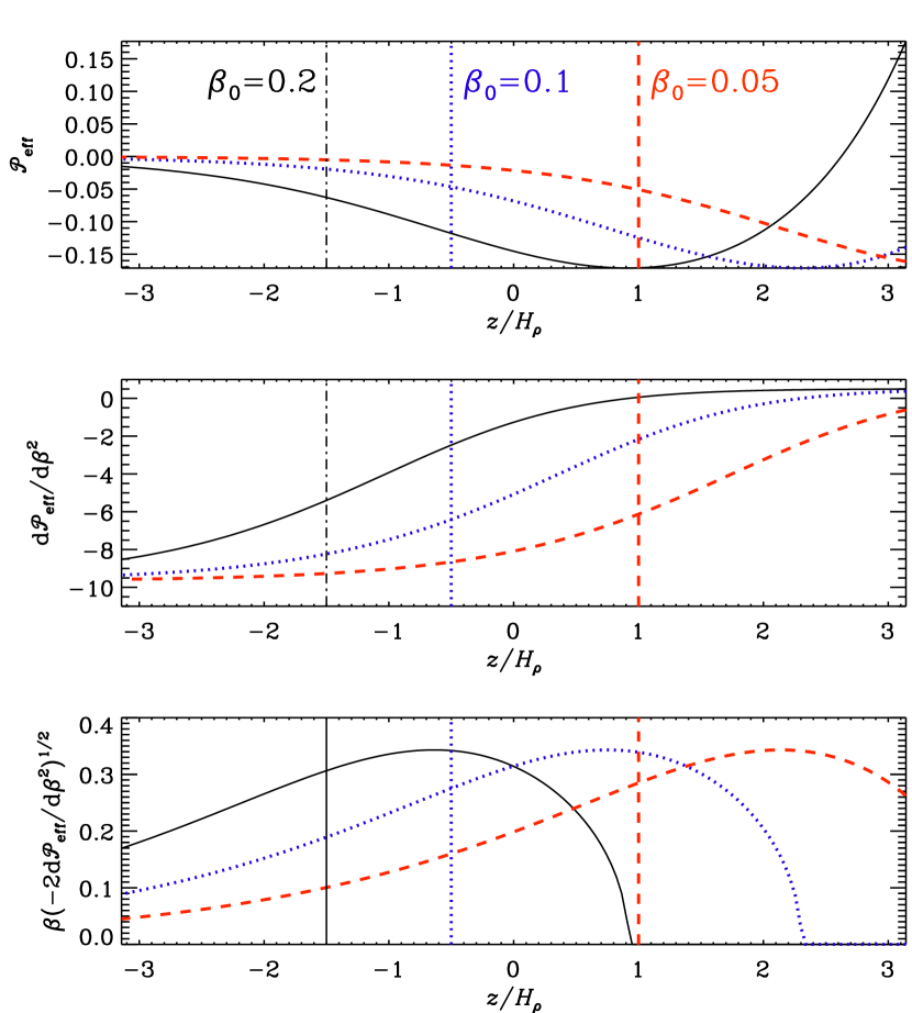
Figure 1.: Profiles of ${\cal P}_{\rm eff}$, ${\rm d}{}{\cal P}_{\rm eff}/{\rm d}{}\beta^{2}$, and $\beta(-2{\rm d}{}{\cal P}_{\rm eff}/{\rm d}{}\beta^{2})^{1/2}$ for fit parameters $q_{\rm p0}=20$ and $\beta_{\rm p}=0.167$, and the three field strengths $B_{0}/B_{\rm eq0}=0.05$, 0.1, and 0.2 within the $z$ range from $-\pi$ to $\pi$, which is consistent with some of the models discussed below. The vertical lines of similar line types give the location where the unstable eigenmodes reaches its peak. MF˙init

Notice first of all that all three curves of ${\cal P}_{\rm eff}$ have minima with left flanks (negative slopes) within the domain. As the imposed field is increased, these curves shift downward (smaller values of $z$). Thus, we should expect the peak of the instable eigenmode to appear somewhere along the left flanks of these curves and that these peaks move further down as the imposed field is increased. This is qualitatively reproduced by the DNS and MFS discussed below, except that the location is consistently a certain distance below the position where the left flanks have their steepest gradient. On the other hand, as is evident from the middle panel of Figure MF_init, the largest value of ${\rm d}{}{\cal P}_{\rm eff}/{\rm d}{}\beta^{2}$ is always achieved at the bottom of the domain. However, the growth rate of NEMPI has still a factor proportional to $v_{\rm A}=u_{\rm rms}\beta$ in front of it; see Equation (disper). This then confines the instability to a narrow strip within the domain. In the third panel of Figure MF_init we plot therefore also $\beta(-2{\rm d}{}{\cal P}_{\rm eff}/{\rm d}{}\beta^{2})^{1/2}$, and their extrema are now only slightly above the location where DNS and MFS show a peak in the eigenfunction. The reason for the remaining discrepancy is not well understood at present.

3 Onset and saturation of NEMPI in DNS

DNS

3.1 Isothermal setup in DNS

model

Following the earlier work of Brandenburg et al. (2011) and Kemel et al. (2012a), we solve the equations for the velocity $U$, the magnetic vector potential $A$, and the density $\rho$,

$$\rho{{\rm D}{}\mbox{\boldmath$U$}{}\over{\rm D}{}t}=-c_{\rm s}^{2}\mbox{\boldmath$\nabla$}{}\rho+\mbox{\boldmath$J$}{}\times\mbox{\boldmath$B$}{}+\rho(\mbox{\boldmath$f$}{}+\mbox{\boldmath$g$}{})+\mbox{\boldmath$\nabla$}{}\cdot(2\nu\rho\mbox{\boldmath${\sf S}$}{}),$$ (15)

$${\partial\mbox{\boldmath$A$}{}\over\partial t}=\mbox{\boldmath$U$}{}\times\mbox{\boldmath$B$}{}+\eta\nabla^{2}\mbox{\boldmath$A$}{},$$ (16)

$${\partial\rho\over\partial t}=-\mbox{\boldmath$\nabla$}{}\cdot\rho\mbox{\boldmath$U$}{},$$ (17)

where $\nu$ is the kinematic viscosity, $\eta$ is the magnetic diffusivity due to Spitzer conductivity of the plasma, $\mbox{\boldmath$B$}{}=\mbox{\boldmath$B$}{}_{0}+\mbox{\boldmath$\nabla$}{}\times\mbox{\boldmath$A$}{}$ is the magnetic field, $\mbox{\boldmath$B$}{}_{0}=(0,B_{0},0)$ is the imposed uniform field, $\mbox{\boldmath$J$}{}=\mbox{\boldmath$\nabla$}{}\times\mbox{\boldmath$B$}{}/\mu_{0}$ is the current density, $\mu_{0}$ is the vacuum permeability, ${\sf S}_{ij}={\textstyle{1\over 2}}(U_{i,j}+U_{j,i})-{\textstyle{1\over 3}}\delta_{ij}\mbox{\boldmath$\nabla$}{}\cdot\mbox{\boldmath$U$}{}$ is the traceless rate of strain tensor, and commas denote partial differentiation. The forcing function $f$ consists of random, white-in-time, plane non-polarized waves with a certain average wavenumber. The turbulent rms velocity is approximately independent of $z$ with $u_{\rm rms}=\langle\mbox{\boldmath$u$}{}^{2}\rangle^{1/2}\approx 0.1\,c_{\rm s}$. The gravitational acceleration $\mbox{\boldmath$g$}{}=(0,0,-g)$ is chosen such that $k_{1}H_{\rho}=1$, so the density contrast between bottom and top is $\exp(2\pi)\approx 535$. Here, $H_{\rho}=c_{\rm s}^{2}/g$ is the density scale height. We consider a domain of size $L_{x}\times L_{y}\times L_{z}$ in Cartesian coordinates $(x,y,z)$, with periodic boundary conditions in the $x$ and $y$ directions and stress-free perfectly conducting boundaries at top and bottom ($z=\pm L_{z}/2$). In all cases, we use a scale separation ratio $k_{\rm f}/k_{1}$ of 30, a fluid Reynolds number $\mbox{\rm Re}\equiv u_{\rm rms}/\nu k_{\rm f}$ of 18, and a magnetic Prandtl number $\mbox{\rm Pr}_{M}=\nu/\eta$ of 0.5. In our units, $\mu_{0}=1$ and $c_{\rm s}=1$. The value of $B_{0}$ is specified in units of the volume averaged value, $B_{\rm eq0}=\sqrt{\mu_{0}\rho_{0}}\,u_{\rm rms}$, where $\rho_{0}=\langle\rho\rangle$ is the volume-averaged density, which is constant in time. In addition to visualizations of the actual magnetic field, we also monitor $\overline{B}_{y}$, which is an average over $y$ and a certain time interval $\Delta t$. Since the simulations are periodic in the $x$ and $y$ directions, we sometimes shift the images such that the peak field strength of NEMPI appears in the middle of the frame.

The simulations are performed with the Pencil Code, which uses sixth-order explicit finite differences in space and a third-order accurate time stepping method. We use a numerical resolution of $256^{3}$ mesh points.

3.2 Results

DNSResults

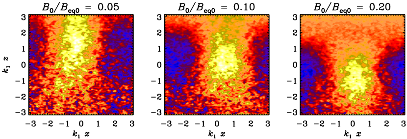
Figure 2.: $\overline{B}_{y}$ from DNS for three values of the imposed field strength at the end of the linear growth phase of NEMPI for $\mbox{\rm Re}_{M}=18$ and $\mbox{\rm Pr}_{M}=0.5$. DNS˙B

In Figure DNS_B we demonstrate that NEMPI can work over a range of field strengths. As we increase the strength of the imposed field, NEMPI develops at progressively greater depth. This result was recently obtained for MFS, but is now for the first time demonstrated in DNS. Figure DNS_grr shows that the growth of the large-scale field $\overline{B}_{1}$ of the magnetic structure is similar for three different field strengths. Here, $\overline{B}_{1}$ has been determined by taking the maximum value of the mean field in the neighborhood of the position where the flux concentration later develops. Note that there is a range over which $\overline{B}_{1}$ grows approximately exponentially, independent of the value of $B_{0}$.

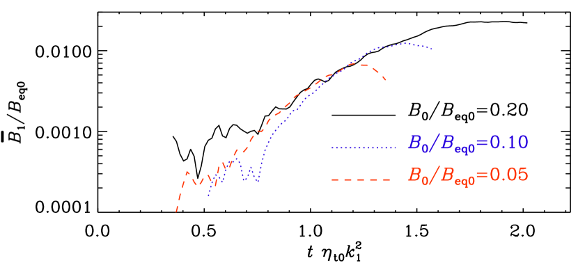
Figure 3.: Growth of the large-scale field strength $\overline{B}_{1}$ at the center of the magnetic structure for three field strengths. DNS˙grr

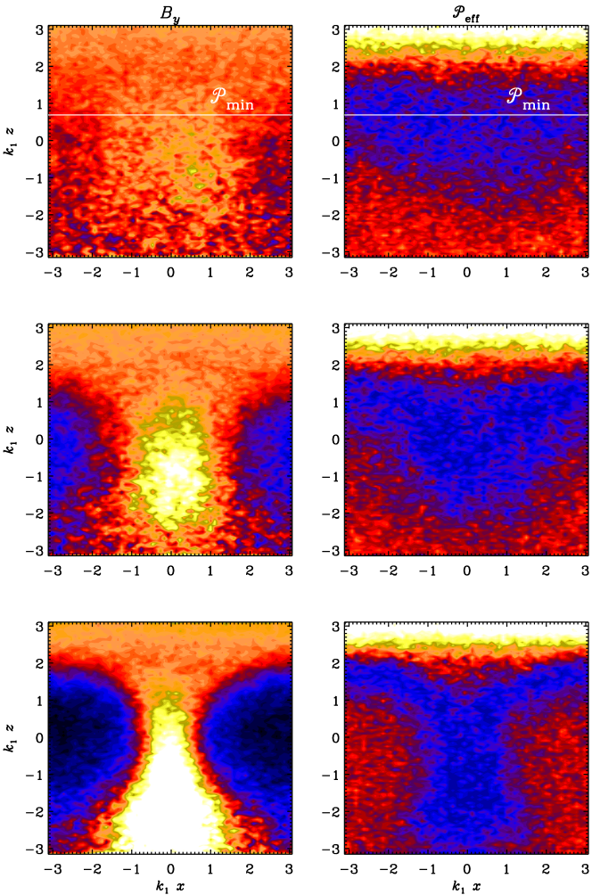
Figure 4.: $\overline{B}_{y}$ and ${\cal P}_{\rm eff}$ from DNS at three times showing the descent of the potato sack feature for $\mbox{\rm Re}_{M}=18$ and $\mbox{\rm Pr}_{M}=0.5$. DNS˙P

In Figure DNS_P we show $\overline{B}_{y}$ at early, intermediate, and late stages of the saturation process (left), and compare with visualizations of ${\cal P}_{\rm eff}$ at the same times. Here, ${\cal P}_{\rm eff}={\textstyle{1\over 2}}(1-q_{\rm p})\beta^{2}$, where $q_{\rm p}(\beta)$ with $\beta=\overline{B}/B_{\rm eq}$ is evaluated from

$$q_{\rm p}=-2\Delta\overline{\Pi}_{xx}^{\rm f}/\overline{\mbox{\boldmath$B$}}{}^{2},$$ (18)

for $\mbox{\boldmath$B$}{}_{0}=(0,B_{0},0)$, and

$$\Delta\overline{\Pi}_{ii}^{\rm f}=\overline{\rho}\,(\overline{u_{i}^{2}}-\overline{u_{0i}^{2}})+{\textstyle{1\over 2}}(\overline{\bm{b}^{2}}-\overline{\bm{b}_{0}^{2}})-(\overline{b_{i}^{2}}-\overline{b_{0i}^{2}}),\ilabel{Pi_{i}i}$$ (19)

is applied to the $xx$ component of the total stress from the fluctuating velocity and magnetic fields. In Equation (Pi_ii) no summation over the repeated index $i$ is assumed.

In Figure DNS_P, blue shades correspond to low values of ${\cal P}_{\rm eff}$ and occur around the minimum line (marked in white) where ${\cal P}_{\rm eff}={\cal P}_{\rm min}$. As time progresses, low values of ${\cal P}_{\rm eff}$ are also found at greater depth as the magnetic flux concentration descends. The fact that there is a clear spatial correlation between $\overline{B}_{y}$ and ${\cal P}_{\rm eff}$ provides strong evidence that the interpretation of the formation of structures in the stratified turbulence simulations in terms of NEMPI is indeed the correct one.

The descending structures have previously been referred to as potato sack structures (Brandenburg et al., 2011), because of their widening cross-section with greater depth. When such structures were first seen in MFS (Brandenburg et al., 2010), they were originally thought to be artifacts of the model that one would not expect to see in the Sun. However, such structures were later also found in DNS (Brandenburg et al., 2011), highlighting therefore the strong predictive power of MFS.

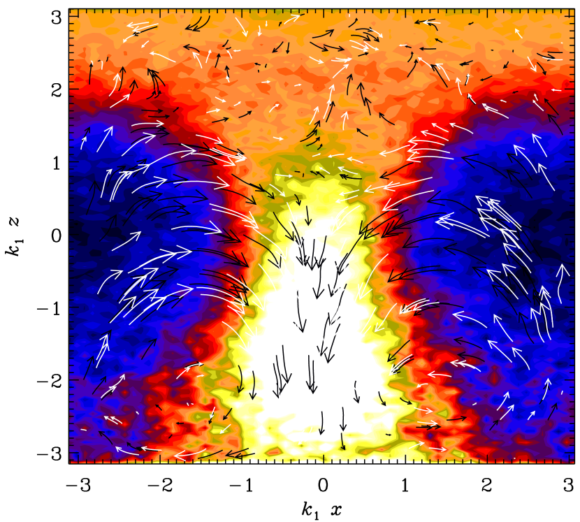
Figure 5.: Vectors of $\overline{\bm{U}}$ together with a color/grey scale representation of $\overline{B}_{y}$ from DNS at a late time for $\mbox{\rm Re}_{M}=18$ and $\mbox{\rm Pr}_{M}=0.5$. DNS˙U

Visualizations of the resulting mean flow $\overline{\bm{U}}$ are shown in Figure DNS_U as vectors. The flow shows a convergent shape toward the magnetic structures. It is interesting to note that such convergent flow structures are now also seen in local helioseismic flow measurements around active regions (Hindman, Haber, and Toomre, 2009). In this connection it is instructive to discuss the somewhat peculiar shape of such a structure that widens as it descends. Normally, in a strongly stratified atmosphere, descending structures get compressed and become narrower, but this is not seen in the present visualizations. As already argued in Brandenburg et al. (2012), this is because the boundaries of these structures do not coincide with material lines, so the mass is not conserved inside them and can leak through the boundaries. Indeed, these structures grow as they descend, and may become amenable to helioseismic detection; cf. Ilonidis, Zhao, and Kosovichev (2011). This phenomenon is well known in the description of turbulent plumes as a model of turbulent downdrafts in convection (Rieutord & Zahn, 1995). Such structures are known to widen as a result of entrainment. The sinking behavior of these apparently disconnected flow structures can be explained as follows: while inflows dominate downflows throughout the whole lifespan of the field concentration, in the initial stage the former can drag in a large fraction of the surrounding magnetic field, overcompensating the losses by downflows. However as the environment gets depleted, this dynamical balance shifts and the structures start moving downwards.

3.3 Mean-field coefficients from DNS

In earlier work by Kemel et al. (2012b), the parameters $q_{\rm p0}=40$ and $\beta_{\rm p}=0.05$, corresponding to $\beta_{\star}=0.32$, were used. Those values are compatible with work by Brandenburg et al. (2012) and Kemel et al. (2012a). However, in the present case we have a larger scale separation ratio, $k_{\rm f}/k_{1}=30$, for which these parameters have not yet been determined. In the Figure DNS_qpc we show the functional form of ${\cal P}_{\rm eff}(\beta)$ for the present case with $k_{\rm f}/k_{1}=30$, $\mbox{\rm Re}_{M}=18$, and $\mbox{\rm Pr}_{M}=0.5$. Here we have followed the method described in Brandenburg et al. (2012); see their Eq. (17). For the present model we find as fit parameters $q_{\rm p0}=20$ and $\beta_{\rm p}=0.167$, which corresponds to $\beta_{\star}=0.75$.

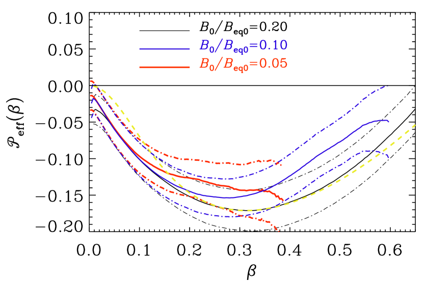
Figure 6.: ${\cal P}_{\rm eff}(\beta)$ for the DNS used in this paper with $k_{\rm f}/k_{1}=30$, $\mbox{\rm Re}_{M}=18$, and $\mbox{\rm Pr}_{M}=0.5$. DNS˙qpc

4 Comparison with MFS

Recently, many aspects of NEMPI seen in the DNS have also been detected in MFS. Establishing the usefulness and limitations of MFS is important, because such models are easier to solve and allow one to explore parameters in regimes where DNS are harder to apply or have not yet been applied in the limited time span since the close correspondence between DNS and MFS was first noted.

In the following we consider two-dimensional mean-field models, in which the presence of $q_{\rm s}$ has no effect on the solutions (Kemel et al., 2012b). Furthermore, we ignore other effects connected with the anisotropy of the turbulence. These effects have previously been found to be weak (Brandenburg et al., 2012; Käpylä et al., 2012).

4.1 Isothermal setup in MFS

modelMFS

In this section we solve the evolution equations for mean velocity $\overline{\bm{U}}$, mean density $\overline{\rho}$, and mean vector potential $\overline{\mbox{\boldmath$A$}}{}$, in the form

$${\partial\overline{\bm{U}}\over\partial t}=-\overline{\bm{U}}\cdot\mbox{\boldmath$\nabla$}{}\overline{\bm{U}}-c_{\rm s}^{2}\mbox{\boldmath$\nabla$}{}\ln\overline{\rho}+\mbox{\boldmath$g$}{}+\overline{\mbox{\boldmath${\cal F}$}}{}_{\rm M}+\overline{\mbox{\boldmath${\cal F}$}}{}_{\rm K},$$ (20)

$${\partial\overline{\rho}\over\partial t}=-\overline{\bm{U}}\cdot\mbox{\boldmath$\nabla$}{}\overline{\rho}-\overline{\rho}\mbox{\boldmath$\nabla$}{}\cdot\overline{\bm{U}},$$ (21)

$${\partial\overline{\mbox{\boldmath$A$}}{}\over\partial t}=\overline{\bm{U}}\times\overline{\mbox{\boldmath$B$}}{}-(\eta_{\it t}+\eta)\overline{\mbox{\boldmath$J$}}{},$$ (22)

where $\overline{\mbox{\boldmath${\cal F}$}}{}_{\rm M}$ is given by

$$\overline{\rho}\,\overline{\mbox{\boldmath${\cal F}$}}{}_{\rm M}=-{\textstyle{1\over 2}}\mbox{\boldmath$\nabla$}{}[(1-q_{\rm p})\overline{\mbox{\boldmath$B$}}{}^{2}]+\overline{\mbox{\boldmath$B$}}{}\cdot\mbox{\boldmath$\nabla$}{}\left[(1-q_{\rm s})\overline{\mbox{\boldmath$B$}}{}\right]\!,\ilabel{efforce}$$ (23)

and

$$\overline{\mbox{\boldmath${\cal F}$}}{}_{\rm K}=(\nu_{\rm t}+\nu)\left(\nabla^{2}\overline{\bm{U}}+{\textstyle{1\over 3}}\mbox{\boldmath$\nabla$}{}\mbox{\boldmath$\nabla$}{}\cdot\overline{\bm{U}}+2\overline{\mbox{\boldmath${\mathsf{S}}$}}{}\mbox{\boldmath$\nabla$}{}\ln\overline{\rho}\right)$$ (24)

is the total (turbulent plus microscopic) viscous force. Here, $\overline{\mathsf{S}}_{ij}={\textstyle{1\over 2}}(\overline{U}_{i,j}+\overline{U}_{j,i})-{\textstyle{1\over 3}}\delta_{ij}\mbox{\boldmath$\nabla$}{}\cdot\overline{\bm{U}}$ is the traceless rate of strain tensor of the mean flow.

We approximate $q_{\rm p}$ by a simple profile that is only a function of the ratio $\beta\equiv|\overline{\mbox{\boldmath$B$}}{}|/B_{\rm eq}$. We use an algebraic fit of the form

$$q_{\rm p}(\beta)={q_{\rm p0}\over 1+\beta^{2}/\beta_{\rm p}^{2}}.\ilabel{qpbeta2}$$ (25)

The function $q_{\rm p}$ quantifies the impact of the mean magnetic field on the effective pressure force.

4.2 Aspects of the MFS

MFSResults

We begin by showing $\overline{B}_{y}$ for three values of the imposed field strength at the end of the linear growth phase of NEMPI. The results are shown in Figures MF_B_stanb and MF_B for two different setups. In the former we use $q_{\rm p0}=20$ and $\beta_{\rm p}=0.167$ for the same $z$ range ($-\pi\leq z/H_{\rho}\leq\pi$) as in the DNS, while in the latter we use $q_{\rm p0}=40$ and $\beta_{\rm p}=0.05$ for somewhat stronger fields and a deeper $z$ range ($0\leq z/H_{\rho}\leq 2\pi$), which is also the fiducial model used by Kemel et al. (2012b). In the former case the growth rate is $\approx 11H_{\rho}^{2}/\eta_{t}$ while in the latter it is $\approx 5.0H_{\rho}^{2}/\eta_{t}$.

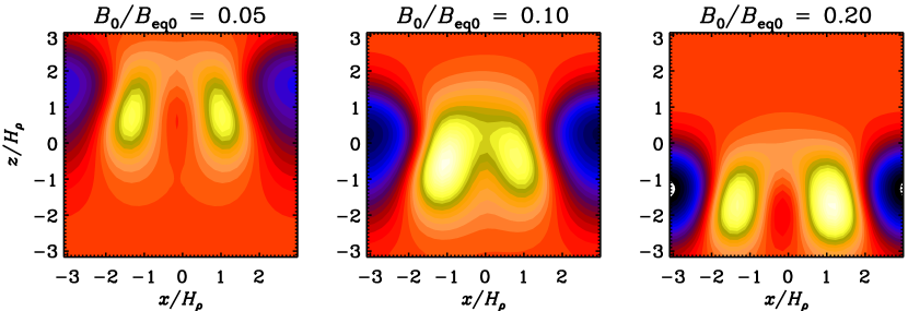
Figure 7.: $\overline{B}_{y}$ from mean-field models for three values of the imposed field strength at the end of the linear growth phase of NEMPI. Here, $q_{\rm p0}=20$ and $\beta_{\rm p}=0.167$, which corresponds to $\beta_{\star}=0.75$. MF˙B˙stanb

Unlike the DNS, the MFS show that in the former series of models with $q_{\rm p0}=20$ and $\beta_{\rm p}=0.167$ the $x$ extend is slightly larger than the optimal horizontal wavelength of the instability, because one sees that some of the structures begin to split into two (Figure MF_B_stanb). This is not the case for the second model with $q_{\rm p0}=40$ and $\beta_{\rm p}=0.05$ (Figure MF_B).

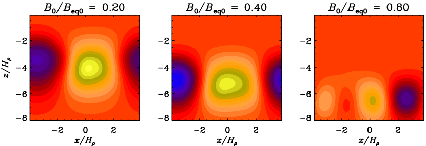
Figure 8.: Similar to Figure MF_B_stanb, but for larger field strengths and vertical domain boundaries that a deeper down, so the magnetic field maxima of the instability fit better into the domain. Here, $q_{\rm p0}=40$ and $\beta_{\rm p}=0.05$, corresponding to $\beta_{\star}=0.32$. MF˙B

Next, we compare $\overline{B}_{y}$ with ${\cal P}_{\rm eff}={\textstyle{1\over 2}}(1-q_{\rm p})\beta^{2}$. Again, there is a close correspondence between the $\overline{B}_{y}$ field and the resulting distribution of ${\cal P}_{\rm eff}$; see Figure MF_P. Here, $q_{\rm p}(\beta)$ is evaluated from the assumed fit formula given by Equation (qpbeta2). Furthermore, there is a close correspondence between regions of enhanced magnetic field and enhanced density; see Figure MF_R.

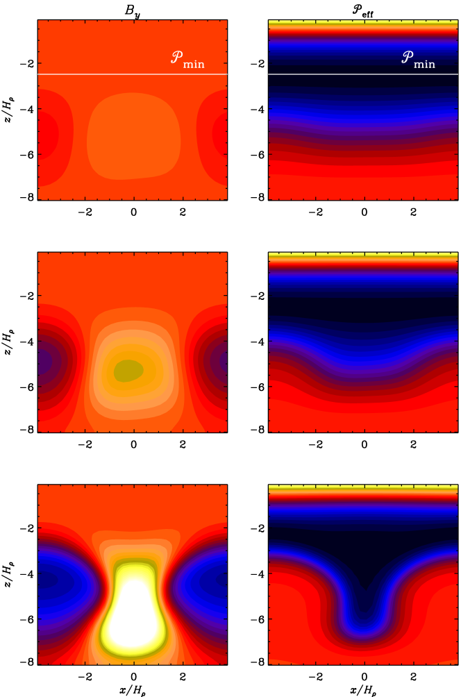
Figure 9.: $\overline{B}_{y}$ and ${\cal P}_{\rm eff}$ from mean-field models at three times. MF˙P

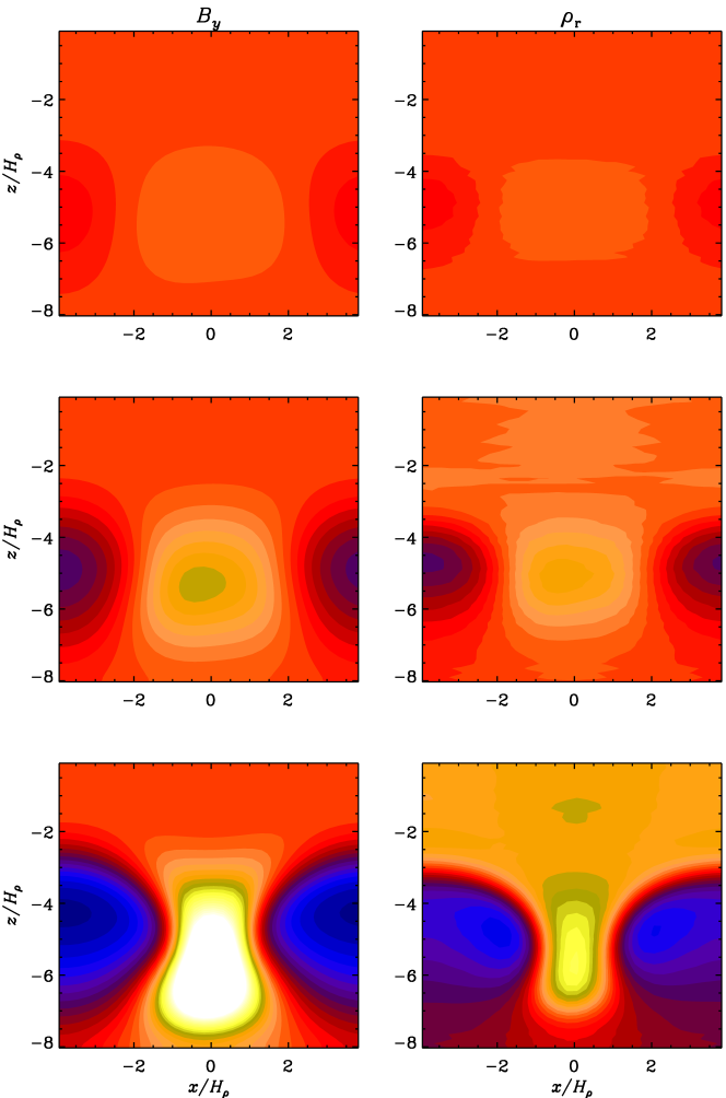
Figure 10.: $\overline{B}_{y}$ compared with $\overline{\rho}$ for three different times. MF˙R

5 Conclusions

The present work has demonstrated that NEMPI is able to concentrate the magnetic field into large patches encompassing the size of many turbulent eddies. The physics of this instability is a straightforward extension of the usual magnetic buoyancy instabilities (Parker, 1966, 1979; Hughes & Proctor, 1988; Cattaneo and Hughes, 1988; Wissink et al., 2000; Isobe et al., 2005; Kersalé, Hughes, and Tobias, 2007), except that the sign of the buoyancy force is reversed in a regime of intermediate field strength. We have here re-examined the simple case of an isothermal layer in which NEMPI can in principle occur at any depth whose value is determined by the strength of the imposed field. Our new DNS have verified that the growth rate is indeed independent of the strength of the imposed field, provided the peak of the instability fits still comfortably within the domain. During the subsequent nonlinear evolution of the instability, the overall density stratification readjusts, allowing the magnetic field concentrations to move further down. It is important to realize that the resulting structures are subject to significant turbulent entrainment (Rieutord & Zahn, 1995), so their boundaries are not closed. The agreement with corresponding mean field models is astounding and much more convincing than what has so been possible to demonstrate in mean-field dynamo theory. Mean-field models provide therefore a strong source of guidance when designing new setups for DNS.

While NEMPI now begins to be fairly well understood for isothermal models, more work is required for non-isothermal ones. In that case, the density scale height is no longer constant and the degree of stratification is much stronger at the top than in deeper layers. The simple result that the instability can occur at any height, depending just on the strength of the imposed field, is then no longer valid. At the same time, there is another perhaps more important aspect, namely the possibility of other instabilities. One of them is connected with the suppression of turbulent convective energy flux by the mean magnetic field. As shown by Kitchatinov & Mazur (2000), this effect can also lead to magnetic flux concentrations and it may be sustained for much stronger magnetic field strengths, allowing thus the formation of structures in which the magnetic pressure becomes comparable to the ambient gas pressure. There may also be a connection with flux segregation events seen in simulations of magnetoconvection at large aspect ratios (Tao et al., 1998; Kitiashvili et al., 2010), which have already been shown to produce bipolar regions in simulations with radiation transfer (Stein et al., 2011). The study of the possibility of producing sunspots similar to those of Rempel (2011a, b), but without initial flux structures, is now of high priority in the quest for solving the solar dynamo problem in terms of distributed dynamo models in which magnetic activity is explained as a surface phenomenon.

Acknowledgements

Computing resources provided by the Swedish National Allocations Committee at the Center for Parallel Computers at the Royal Institute of Technology in Stockholm and the High Performance Computing Center North in Umeå. This work was supported in part by the European Research Council under the AstroDyn Research Project No. 227952 and the Swedish Research Council under the project grant 621-2011-5076.

Appendix A Growth rate of NEMPI

LinTheo

In this Appendix we derive the growth rate of NEMPI neglecting for simplicity dissipation processes, using anelastic approximation for small Mach numbers and assuming the density hight, $H_{\rho}$ to be constant and $\mu_{0}=1$. Let us rewrite the equation of motion in the following form

$${\partial\overline{\bm{U}}(t,x,z)\over\partial t}=-\mbox{\boldmath$\nabla$}{}\left({p_{\rm tot}\over\overline{\rho}}\right)+{p_{\rm tot}\over\overline{\rho}H_{\rho}}\hat{\bm{z}}+\mbox{\boldmath$g$}{},\ilabel{A1}$$ (26)

where $\hat{\bm{z}}$ is the vertical unit vector, $p_{\rm tot}=\overline{p}+p_{\rm eff}$ is the total pressure (the sum of the mean gas pressure, $\overline{p}$, and the effective magnetic pressure, $p_{\rm eff}$), and we took into account that mean magnetic field is independent on $y$, so that the mean magnetic tension vanishes. We also used an identity:

$$\mbox{\boldmath$\nabla$}{}\left({p_{\rm tot}\over\overline{\rho}}\right)={\mbox{\boldmath$\nabla$}{}p_{\rm tot}\over\overline{\rho}}+{p_{\rm tot}\over\overline{\rho}H_{\rho}}\hat{\bm{z}},\ilabel{A4}$$ (27)

Taking twice curl of Equation (A1) we obtain

$${\partial\over\partial t}\left(\Delta-{\nabla_{z}\over H_{\rho}}\right)\overline{U}_{z}={1\over\overline{\rho}H_{\rho}}\Delta_{\perp}p_{\rm eff},\ilabel{A2}$$ (28)

where $\Delta_{\perp}=\Delta-\nabla_{z}^{2}$ and we have used Equation (divu). Introducing a new variable $V_{z}=\sqrt{\overline{\rho}}\,\overline{U}_{z}$, we rewrite Equation (A2) for a new variable:

$${\partial\over\partial t}\left(\Delta-{1\over 4H_{\rho}^{2}}\right)V_{z}={1\over\sqrt{\overline{\rho}}H_{\rho}}\Delta_{\perp}p_{\rm eff}.\ilabel{A5}$$ (29)

Linearizing Equation (A5), and using the linearized induction Equation (induct-eq) we arrive at the following equation:

$${\partial^{2}\over\partial t^{2}}\left(\Delta-{1\over 4H_{\rho}^{2}}\right)V_{z}(t,x,z)=-{2\beta_{0}^{2}\over\overline{\rho}H_{\rho}^{2}}\left.{{\rm d}{}p_{\rm eff}\over{\rm d}{}\beta^{2}}\right|_{\beta_{0}}\Delta_{\perp}V_{z},\ilabel{A6}$$ (30)

where ${\rm d}{}p_{\rm eff}/{\rm d}{}\beta^{2}={\textstyle{1\over 2}}(1-q_{\rm p}-{\rm d}{}q_{\rm p}/{\rm d}{}\ln\beta^{2})B_{0}^{2}/\beta^{2}$, $\beta=\overline{B}/B_{\rm eq}(z)$ and $\beta_{0}=B_{0}/B_{\rm eq0}$. It follows from Equation (A6) that a necessary condition for the large-scale instability is

$$\left.{{\rm d}{}p_{\rm eff}\over{\rm d}{}\beta^{2}}\right|_{\beta_{0}}<0.\ilabel{A10}$$ (31)

For instance, in WKB approximation when $k_{z}\,H_{\rho}\gg 1$, i.e. when the characteristic scale of the spatial variation of the perturbations of the magnetic and velocity fields are much smaller than the density hight length $H_{\rho}$, the growth rate of the instability reads

$$\lambda={\beta_{0}k_{\perp}\over\sqrt{\overline{\rho}_{0}}\,H_{\rho}k}\,\left(-2\left.{{\rm d}{}p_{\rm eff}\over{\rm d}{}\beta^{2}}\right|_{\beta_{0}}\right)^{1/2}.\ilabel{A11}$$ (32)

For an arbitrary $k_{z}\,H_{\rho}$ we seek a solution of Equation (A6) in the form: $V_{z}(t,x,z)=V(z)\exp(\lambda t+ik_{\perp}\,x)$. Introducing new variables:

$$\Psi(R)=\sqrt{R}\,V(z),\quad R(z)={v_{A0}^{2}\over u_{\rm rms}^{2}\beta_{\rm p}^{2}}\,e^{z/H_{\rho}},\ilabel{A7}$$ (33)

we can rewrite Equation (A6) in the form of a 1-D Schrödinger equation for the function $\Psi(R)$:

$${d^{2}\Psi\over dR^{2}}-\tilde{U}(R)\Psi=0,\quad\tilde{U}(R)={k_{\perp}^{2}\over R}\,\left({H_{\rho}^{2}\over R}-{a\,q_{\rm p0}\over(1+R)^{2}}+a\right),\ilabel{A8}$$ (34)

where $\overline{\rho}=\overline{\rho}_{0}\,e^{-z/H_{\rho}}$, $v_{\rm A0}=B_{0}/\sqrt{\overline{\rho}_{0}}$ is the Alfvén speed, the parameter $a$ is

$$a={u_{\rm rms}^{2}\,\beta_{\rm p}^{2}\over\lambda^{2}},\ilabel{A9}$$ (35)

and the potential $\tilde{U}(R)$ has the following asymptotic behavior: $\tilde{U}(R\to 0)=k_{\perp}^{2}H_{\rho}^{2}/R^{2}$ and $\tilde{U}(R\to\infty)=a/R$. For the existing of the instability, the potential $\tilde{U}(R)$ should have a negative minimum. For example, for a long wavelength instability ($k_{\perp}^{2}H_{\rho}^{2}\ll 1$) and when $q_{\rm p0}>1$, the potential $\tilde{U}(R)$ has a negative minimum, and the instability can be excited. When the potential $\tilde{U}(R)$ has a negative minimum and since $\tilde{U}(R\to 0)>0$ and $\tilde{U}(R\to\infty)>0$, there are two points $R_{1}$ and $R_{2}$ (the so-called turning points) in which $\tilde{U}(R)=0$. Using the equations $\tilde{U}(R_{1,2})=0$ and Equations (A8)–(A9) we obtain the growth rate of the instability as

$$\lambda={\beta_{\star}\,u_{\rm rms}\over H_{\rho}}\,{\left[R_{1}R_{2}(2+R_{1}+R_{2})\right]^{1/2}\over(1+R_{1})(1+R_{2})},\ilabel{A12}$$ (36)

where we have used $\beta_{\star}=\beta_{\rm p}\sqrt{q_{\rm p0}}$. Note that Equation (A12) is consistent with the simple estimate (E1).

References

- Brandenburg (2005) Brandenburg, A. 2005, ApJ, 625, 539
- Brandenburg et al. (2011) Brandenburg, A., Kemel, K., Kleeorin, N., Mitra, D., & Rogachevskii, I. 2011, ApJ, 740, L50
- Brandenburg et al. (2012) Brandenburg, A., Kemel, K., Kleeorin, N., & Rogachevskii, I. 2012, ApJ, to be published (arXiv:1005.5700)
- Brandenburg et al. (2010) Brandenburg, A., Kleeorin, N., & Rogachevskii, I. 2010, Astron. Nachr., 331, 5
- Cattaneo and Hughes (1988) Cattaneo, F., Hughes, D. W. 1988, J. Fluid Mech., 196, 323
- Golub et al. (1981) Golub, L., Rosner, R., Vaiana, G. S., & Weiss, N. O. 1981, ApJ, 243, 309
- Hindman, Haber, and Toomre (2009) Hindman, B. W., Haber, D. A., and Toomre, J. 2009, ApJ, 698, 1749
- Hughes & Proctor (1988) Hughes, D. W., & Proctor, M. R. E. 1988, Ann. Rev. Fluid Mech., 20, 187
- Ilonidis, Zhao, and Kosovichev (2011) Ilonidis, S., Zhao, J., Kosovichev, A. 2011, Science, 333, 993
- Isobe et al. (2005) Isobe, H., Miyagoshi, T., Shibata, K., Yokoyama, T. 2005, Nature, 434, 478
- Käpylä et al. (2012) Käpylä, P. J., Brandenburg, A., Kleeorin, N., Mantere, M. J., Rogachevskii, I. 2012, MNRAS, to be published (arXiv:1105.5785)
- Kemel et al. (2012a) Kemel, K., Brandenburg, A., Kleeorin, N., Mitra, D., & Rogachevskii, I. 2012, Sol. Phys., to be published (arXiv:1112.0279)
- Kemel et al. (2012b) Kemel, K., Brandenburg, A., Kleeorin, N., & Rogachevskii, I. 2012, Astron. Nachr., 333, 95
- Kersalé, Hughes, and Tobias (2007) Kersalé, E., Hughes, D. W., Tobias, S. M. 2007, ApJ, 663, L113
- Kitchatinov & Mazur (2000) Kitchatinov, L.L., & Mazur, M.V. 2000, Solar Phys., 191, 325 (KM)
- Kitiashvili et al. (2010) Kitiashvili, I. N., Kosovichev, A. G., Wray, A. A., & Mansour, N. N. 2010, ApJ, 719, 307
- Kleeorin, Mond, and Rogachevskii (1996) Kleeorin, N., Mond, M., Rogachevskii, I. 1996, A&A, 307, 293
- Kleeorin & Rogachevskii (1994) Kleeorin, N., & Rogachevskii, I. 1994, Phys. Rev. E, 50, 2716
- Kleeorin et al. (1989) Kleeorin, N.I., Rogachevskii, I.V., Ruzmaikin, A.A. 1989, Sov. Astron. Lett., 15, 274
- Kleeorin et al. (1990) Kleeorin, N.I., Rogachevskii, I.V., & Ruzmaikin, A.A. 1990, Sov. Phys. JETP, 70, 878
- Parker (1966) Parker, E.N. 1966, ApJ, 145, 811
- Parker (1979) Parker, E. N. 1979, Cosmical magnetic fields (Oxford University Press, New York)
- Rempel (2011a) Rempel, M. 2011a, ApJ, 729, 5
- Rempel (2011b) Rempel, M. 2011b, ApJ, 740, 15
- Rieutord & Zahn (1995) Rieutord, M., & Zahn, J.-P. 1995, A&A, 296, 127
- Rogachevskii & Kleeorin (2007) Rogachevskii, I., & Kleeorin, N. 2007, Phys. Rev. E, 76, 056307
- Stein et al. (2011) Stein, R. F., Lagerfjärd, A., Nordlund, Å., & Georgobiani, D. 2011, Solar Phys., 268, 271
- Tao et al. (1998) Tao, L., Weiss, N. O., Brownjohn, D. P., & Proctor, M. R. E. 1998, ApJ, 496, L39
- Wissink et al. (2000) Wissink, J. G., Hughes, D. W., Matthews, P. C., & Proctor, M. R. E. 2000, MNRAS, 318, 501