The effective Hamiltonian in curved quantum waveguides under mild regularity assumptions

Abstract

The Dirichlet Laplacian in a curved three-dimensional tube built along a spatial (bounded or unbounded) curve is investigated in the limit when the uniform cross-section of the tube diminishes. Both deformations due to bending and twisting of the tube are considered. We show that the Laplacian converges in a norm-resolvent sense to the well known one-dimensional Schrödinger operator whose potential is expressed in terms of the curvature of the reference curve, the twisting angle and a constant measuring the asymmetry of the cross-section. Contrary to previous results, we allow the reference curves to have non-continuous and possibly vanishing curvature. For such curves, the distinguished Frenet frame standardly used to define the tube need not exist and, moreover, the known approaches to prove the result for unbounded tubes do not work. Our main ideas how to establish the norm-resolvent convergence under the minimal regularity assumptions are to use an alternative frame defined by a parallel transport along the curve and a refined smoothing of the curvature via the Steklov approximation.

1 Introduction

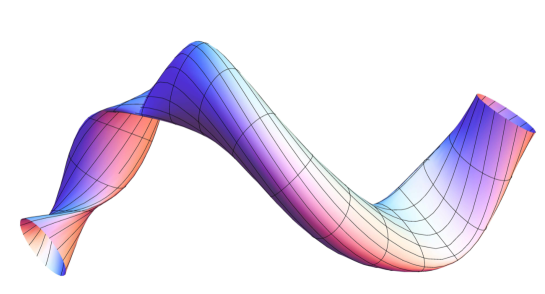
This paper is concerned with the singular operator limit for the Dirichlet Laplacian in a three-dimensional non-self-intersecting curved tube (cf Figure 1) when its two-dimensional cross-section shrinks to a point. The tube $\Omega_{\varepsilon}$ is constructed by translating and rotating the cross-section along a spatial curve $\Gamma$ and the limit is realized by homothetically scaling a fixed cross-section $\omega$ by a small positive number $\varepsilon$. Without loss of generality, we assume that the curve is given by its arc-length parameterization $\Gamma:I\to\mathbb{R}^{3}$, where the open interval $I\subset\mathbb{R}$ is allowed to be arbitrary: finite, infinite or semi-infinite. Geometrically, $\Omega_{\varepsilon}$ collapses to $\Gamma$ as $\varepsilon\to 0$. We are interested in how and when the three-dimensional Dirichlet Laplacian $-\Delta_{D}^{\Omega_{\varepsilon}}$ can be approximated by a one-dimensional operator $H_{\mathrm{eff}}$ on the curve.

Figure 1: The geometry of a quantum waveguide. Twisting and bending are demonstrated on the left and right part of the figure, respectively.

We start with some more or less obvious observations.

• Since we deal with unbounded operators, the convergence of $-\Delta_{D}^{\Omega_{\varepsilon}}$ to $H_{\mathrm{eff}}$ is understood through a convergence of their resolvents.

• The Dirichlet boundary conditions imply that the spectrum of $-\Delta_{D}^{\Omega_{\varepsilon}}$ explodes as $\varepsilon\to 0$. It is just because the first eigenvalue of the Dirichlet Laplacian in the scaled cross-section $\varepsilon\omega:=\{\varepsilon t\,|\,t\in\omega\}$ equals $\varepsilon^{-2}E_{1}$, where $E_{1}$ is the first eigenvalue of the Dirichlet Laplacian in the fixed cross-section $\omega$. Hence, a normalization $-\Delta_{D}^{\Omega_{\varepsilon}}-\varepsilon^{-2}E_{1}$ is in order to get a non-trivial limit.

• Finally, since the configuration spaces $\Omega_{\varepsilon}$ and $\Gamma$ have different dimensions, a suitable identification of respective Hilbert spaces of $-\Delta_{D}^{\Omega_{\varepsilon}}$ and $H_{\mathrm{eff}}$ is required. This is achieved by using a unitary transform that identifies $L^{2}(\Omega_{\varepsilon})$ with $L^{2}(I\times\omega)$ and by considering $H_{\mathrm{eff}}$ as acting on the subspace of $L^{2}(I\times\omega)$ spanned by functions of the form $\varphi\otimes\mathcal{J}_{1}$ on $I\times\omega$, where $\mathcal{J}_{1}$ denotes the positive normalized eigenfunction of $-\Delta_{D}^{\omega}$ corresponding to $E_{1}$.

Taking these remarks into account, we can write the convergence result as follows:

$$-\Delta_{D}^{\Omega_{\varepsilon}}-\varepsilon^{-2}E_{1}\ \xrightarrow[]{\varepsilon\to 0}\ H_{\mathrm{eff}}^{F}:=-\Delta_{D}^{I}-\frac{\kappa^{2}}{4}+C_{\omega}\,(\dot{\theta}_{F}-\tau)^{2}\,.$$ (1.1)

Here $\kappa:=|\ddot{\Gamma}|$ and $\tau:=\kappa^{-2}\det(\dot{\Gamma},\ddot{\Gamma},\dddot{\Gamma})$ denote respectively the curvature and torsion of $\Gamma$, $\theta_{F}$ is an angle function defining the rotation of $\varepsilon\omega$ with respect to the Frenet frame of $\Gamma$ and $C_{\omega}:=\|\partial_{\alpha}\mathcal{J}_{1}\|_{L^{2}(\omega)}$, with $\partial_{\alpha}$ denoting the angular derivative in $\mathbb{R}^{2}$.

The convergence (1.1) can be employed as a way to approximate the three-dimensional dynamics of an electron constrained to a curved quantum waveguide by the effective one-dimensional Hamiltonian $H_{\mathrm{eff}}^{F}$ on the reference curve. The Dirichlet Laplacian on the interval $I$ represents the kinetic energy of the free motion on the reference curve (indeed, $-\Delta_{D}^{I}$ is unitarily equivalent to the Laplace-Beltrami operator on $\Gamma$). The additional potential of $H_{\mathrm{eff}}^{F}$ clearly consists of two competing terms: the negative one induced by curvature and the positive one due to torsion. They respectively represent the opposite effects of bending and twisting in quantum waveguides, cf [17].

1.1 Known results and why we write this paper

The result (1.1) is well known, it has been established in various settings and with different methods during the last two decades. As the first rigorous result, let us mention the classical paper [9] of Duclos and Exner, where the norm-resolvent convergence of (1.1) is proved under quite restrictive hypotheses $\Gamma\in C^{4}$ and $\omega$ being a disc (so that $C_{\omega}=0$). More precise results about the limit (for instance, uniform convergence of eigenfunctions) in arbitrary dimensions are established by Freitas and Krejčiřík in [11], but the cross-section is still assumed to be rotated along $\Gamma$ in such a way that $\dot{\theta}_{F}=\tau$, so there is no effect of twisting.

The presence of the additional potential term due to twisting in $H_{\mathrm{eff}}^{F}$ was observed for the first time by Bouchitté, Mascarenhas and Trabucho [4]. Contrary to the previous works where operator techniques are used, the authors of [4] use an alternative method of Gamma-convergence, which provides just a strong-resolvent convergence of (1.1) but, on the other hand, enables them to weaken the regularity hypothesis to $\Gamma\in C^{3}$. De Oliveira [6] extended the results of [4] to unbounded tubes and established a norm-resolvent convergence in the bounded case (see also [7, 8]).

Finally, let us mention the series of recent papers [20, 23, 24], where the singular limit of the type (1.1) is attacked by the methods of adiabatic perturbation theory. In fact, the general setting of shrinking tubular neighbourhoods of (infinitely smooth) submanifolds of Riemannian manifolds is considered in these works and the results can be interpreted as a rigorous quantization procedure on the submanifolds.

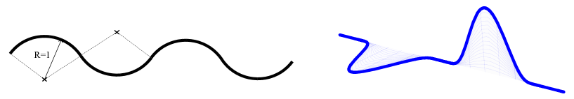
After having provided an extensive literature on the limit (1.1), a question arises why we still consider the problem in the present paper. In fact, the issue we would like to address here is about the optimal regularity conditions under which the effective approximation (1.1) holds. We are motivated by the fact that the known existing results mentioned above do not cover physically interesting curves with merely continuous or even discontinuous curvature (cf Figure 2).

Figure 2: Examples of curves with discontinuous curvature (on the left) and with infinitely smooth curvature but still without the Frenet frame (on the right).

Furthermore, it is a standard hypothesis in the literature about quantum waveguides that the first three derivatives of the reference curve $\Gamma$ exist and are linearly independent, so that the torsion and the distinguished Frenet frame exist. However, this is meaningful only for curves which are three times differentiable and have nowhere vanishing (differentiable) curvature $\kappa$. We find the latter as a very restrictive requirement, even for infinitely smooth curves (cf Figure 2). Indeed, the torsion $\tau$ is not well defined for such curves, so that the limit (1.1) with the effective Hamiltonian $H_{\mathrm{eff}}^{F}$ is meaningless. Partial attempts to overcome this technical condition can be found in [3, 5]. In this paper we provide a complete answer by considering waveguides built along any twice differentiable curves, with the boundedness of $\kappa$ being the only hypothesis. Our assumptions are very natural and in fact intrinsically necessary for the construction of the waveguide as a regular Riemannian manifold.

Finally, the Gamma-convergence method of [4, 6], which seems to work under less restrictive regularity once the technical difficulty of the non-existence of the Frenet frame is overcome, implies only (unless the waveguide is bounded [6]) a strong-resolvent convergence for (1.1). Furthermore, it does not provide any information about the convergence rate. In addition to the regularity issues mentioned above, our goal is therefore to use operator methods instead of the Gamma-convergence, establish (1.1) in the norm-resolvent sense and get a control on the convergence rate.

1.2 The content of the paper

The organization of this paper is as follows.

In the following Section 2 we explain our strategy to handle the singular limit under mild regularity hypotheses and state the main result of this paper (Theorem 2.1).

We postpone a precise definition of a simultaneously twisted and bent waveguide and of the associated Dirichlet Laplacian till Section 3. For reasons mentioned above, we construct the waveguide by using an alternative frame defined by parallel transport along the curve instead of the usual Frenet frame. Since it seems that this frame is not as well known as the Frenet one, and since we want to include more general curves than those usually considered in differential geometry, we decided to include Section 3.1, where we thoroughly describe the construction of the frame under our mild regularity conditions.

The main idea of the present paper consists in smoothing non-differentiable quantities by means of the so-called Steklov approximation (see (2.5) below). This procedure is in detail explained in Section 4.

The proof of Theorem 2.1 is given in Section 5. Since it is rather long and technically involved, we divide the proof into several auxiliary lemmata and the section into corresponding subsections.

The paper is concluded in Section 6 by discussing optimality of our results.

2 Our strategy and the main result

Our strategy how to achieve the objectives sketched in Introduction is based on the following ideas:

1. Use the frame defined by the parallel transport instead of the Frenet frame. This alternative frame is known to exist for any curve of class $C^{2}$, cf [2]. We generalize the construction to the curves that merely belong to the Sobolev space $W_{\mathrm{loc}}^{2,\infty}$.

2. Work exclusively with the quadratic forms associated with the operators. More specifically, we adapt the elegant method of Friedlander and Solomyak [13, 12] to deduce the norm-resolvent convergence from a convergence of quadratic forms.

Even if one implements these ideas, the standard operator approach to the thin-cross-section limit in quantum waveguides (see, e.g., [9]) still requires certain differentiability of curvature $\kappa$ (which is just bounded under our hypotheses). To see it, we sketch the standard strategy now.

First, one uses curvilinear coordinates, which induce the unitary transform

$$U_{1}:L^{2}(\Omega_{\varepsilon})\to L^{2}\big{(}I\times\omega,\varepsilon^{2}\;\!h(s,t)\;\!ds\;\!dt\big{)},$$ (2.1)

where the Jacobian $\varepsilon^{2}h$ is standardly expressed in terms of $\kappa$ and $\theta_{F}$. In our more general setting enabled by the strategy (I) above, we have

$$h(\cdot,t):=1-\varepsilon\,t_{1}\,(k_{1}\cos\theta-k_{2}\sin\theta)-\varepsilon\,t_{2}\,(k_{1}\sin\theta+k_{2}\cos\theta)\,,$$ (2.2)

where $k_{1},k_{2}$ are curvature functions computed with respect to our relatively parallel frame and $\theta$ is an angle function defining the rotation of the cross-section $\varepsilon\omega$ with respect to this frame. We have $\kappa^{2}=k_{1}^{2}+k_{2}^{2}$ and, if the Frenet frame exists, our frame is rotated with respect to the Frenet frame by the angle given by a primitive of torsion $\tau$ (cf (3.4) below). Consequently, in our more general setting, the difference $\dot{\theta}_{F}-\tau$ in (1.1) is to be replaced by $\dot{\theta}$ and the effective Hamiltonian reads

$$H_{\mathrm{eff}}:=-\Delta_{D}^{I}-\frac{\kappa^{2}}{4}+C_{\omega}\;\!\dot{\theta}^{2}.$$ (2.3)

We emphasize that this operator coincides with $H_{\mathrm{eff}}^{F}$ introduced in (1.1) if $\Gamma$ possesses the Frenet frame but, contrary to $H_{\mathrm{eff}}^{F}$, it is well defined even if the torsion $\tau$ does not exist.

Second, to recover the curvature term in the effective potential of (1.1), one also performs the unitary transform

$$U_{2}:L^{2}\big{(}I\times\omega,\varepsilon^{2}\;\!h(s,t)\;\!ds\;\!dt\big{)}\to L^{2}(I\times\omega):\left\{\psi\mapsto\varepsilon\;\!\sqrt{h}\;\!\psi\right\}\,.$$ (2.4)

The composition $U:=U_{2}U_{1}$ clearly identifies the geometrically complicated Hilbert space $L^{2}(\Omega_{\varepsilon})$ with the simple $L^{2}(I\times\omega)$. The standard procedure consists in transforming $-\Delta_{D}^{\Omega_{\varepsilon}}$ with help of $U$ to a unitarily equivalent operator on $L^{2}(I\times\omega)$ and prove the norm-resolvent convergence for the transformed operator. However, $U$ does not leave the form domain $W_{0}^{1,2}(I\times\omega)$ invariant if $k_{1},k_{2}$ are not differentiable in a suitable sense.

The last difficulty is overcome in this paper by the following trick:

• Replace the curvature functions in (2.2) by their $\varepsilon$-dependent mollifications ($\mu\in\{1,2\}$)

  $$k_{\mu}^{\varepsilon}(s):=\frac{1}{\delta(\varepsilon)}\int_{s-\frac{\delta(\varepsilon)}{2}}^{s+\frac{\delta(\varepsilon)}{2}}k_{\mu}(\xi)\,d\xi\,,$$ (2.5)

  where $\delta$ is a continuous function such that both $\delta(\varepsilon)$ and $\varepsilon\;\!\delta(\varepsilon)^{-1}$ tend to zero as $\varepsilon\to 0$.

Then everything works very well (although the overall procedure is technically much more demanding) because the longitudinal derivative of the mollified $h$ involves the terms $\varepsilon\dot{k}_{\mu}^{\varepsilon}$ which vanish as $\varepsilon\to 0$, even if $\dot{k}_{\mu}^{\varepsilon}$ diverge in this limit. In more intuitive words, (2.5) can be understood in a sense as that the curve is smoothed on a scale small compared to the curvature of the curve, but large compared to the diameter of the cross-section of the waveguide.

The mollification (2.5) is sometimes referred to as the Steklov approximation in Russian literature (see, e.g., [1]). At a step of our proof, we shall also need to mollify the derivative of the angle function $\theta$.

Before stating the main result of the paper, let us now carefully write down all the hypotheses we need to derive it, although some of the quantities appearing in the assumptions will be properly defined only later.

Assumption 1.

Let $\Gamma:I\rightarrow\mathbb{R}^{3}$ be a unit-speed spatial curve, where the interval $I\subset\mathbb{R}$ is finite, semi-infinite or infinite, satisfying

• $\Gamma\in W^{2,\infty}_{\mathrm{loc}}(I;\mathbb{R}^{3})$  and  $\kappa:=|\ddot{\Gamma}|\in L^{\infty}(I)$.

Further, let $\omega$ be a bounded open connected subset of $\mathbb{R}^{2}$ and let $\theta:I\to\mathbb{R}$ be the angle describing the rotation of the waveguide cross-section $\varepsilon\omega$ with respect to the relatively parallel adapted frame constructed along $\Gamma$ satisfying

• $\theta\in W^{1,\infty}_{\mathrm{loc}}(I)$  and  $\dot{\theta}\in L^{\infty}(I)$.

Finally, we assume

• $\Omega_{\varepsilon}$ does not overlap itself for all sufficiently small $\varepsilon$.

The conditions stated in Assumption 1 are quite week and in fact very natural for the construction of the waveguide $\Omega_{\varepsilon}$ and for obtaining reasonable spectral consequences from (1.1) (cf Section 6 for further discussion). Unfortunately, for making our strategy to work in the case of unbounded waveguides, we also need to assume the following (seemingly technical) hypothesis.

Assumption 2.

For any $f\in L_{\mathrm{loc}}^{\infty}(I)$, let us define

$$\sigma_{f}(\delta(\varepsilon)):=\sup_{n\in\mathbb{Z}}\sqrt{\sup_{|\eta|\leq\frac{\delta(\varepsilon)}{2}}\int_{n}^{n+1}\ \left|f(s)-f(s+\eta)\right|^{2}ds}\,.$$ (2.6)

where $\varepsilon\mapsto\delta(\varepsilon)$ is some continuous function vanishing with $\varepsilon$. To give a meaning to (2.6) for $I\not=\mathbb{R}$, we assume that $f$ is extended from $I$ to $\mathbb{R}$ by zero. We make the following two hypotheses

$$\lim_{\varepsilon\to 0}\sigma_{k}(\delta(\varepsilon)):=\lim_{\varepsilon\to 0}\sum_{\mu=1,2}\sigma_{k_{\mu}}(\delta(\varepsilon))=0\,,$$ (2.7)

$$\lim_{\varepsilon\to 0}\sigma_{\dot{\theta}}(\tilde{\delta}(\varepsilon))=0\,.$$ (2.8)

for some positive continuous functions $\delta,\tilde{\delta}$ satisfying

$$\lim_{\varepsilon\to 0}\delta(\varepsilon)=0\,,\qquad\lim_{\varepsilon\to 0}\frac{\varepsilon}{\delta(\varepsilon)}=0\,,\qquad\lim_{\varepsilon\to 0}\tilde{\delta}(\varepsilon)=0\,.$$ (2.9)

Assumption 2 is satisfied for a wide class of reference curves $\Gamma$ and rotation angles $\theta$. First of all, let us emphasize that it always holds whenever $I$ is bounded. Indeed, this is a consequence of the more general fact that Assumption 2 holds provided that (the extensions of) the representants of $f$ are square-integrable functions on $\mathbb{R}$. As other sufficient conditions which guarantee the validity of Assumption 2, let us mention that it holds whenever the representants are either Lipschitz, or just uniformly continuous, or periodic, etc. In any case, it is a non-void hypothesis for unbounded $I$ only, when it becomes important to have a control over the behaviour of $k_{1},k_{2}$ and $\dot{\theta}$ at infinity.

Now we are in a position to state the main result of this paper.

Theorem 2.1.

Let Assumption 1 and Assumption 2 hold true. Then there exist positive constants $\varepsilon_{0}$ and $C$ such that for all $\varepsilon\leq\varepsilon_{0}$,

$$\left\|U(-\Delta_{D}^{\Omega_{\varepsilon}}-\varepsilon^{-2}E_{1}-i)^{-1}U^{-1}-(H_{\mathrm{eff}}-i)^{-1}\oplus 0^{\bot}\right\|_{\mathcal{B}(L^{2}(I\times\omega))}\\ \leq C\left(\varepsilon+\varepsilon\;\!\|\dot{k}_{1}^{\varepsilon}\|+\varepsilon\;\!\|\dot{k}_{1}^{\varepsilon}\|+\sigma_{k}(\delta(\varepsilon))+\sigma_{\dot{\theta}}(\tilde{\delta}(\varepsilon))\right)\,,$$ (2.10)

where $0^{\bot}$ denotes the zero operator on the orthogonal complement of the span of $\{\varphi\otimes\mathcal{J}_{1}\,|\,\varphi\in L^{2}(I)\}$ and $U=U_{2}U_{1}$ is the unitary transform composed of (2.1) and (2.4).

Recall that the quantities $\varepsilon\|\dot{k}_{1}^{\varepsilon}\|_{\infty}$ and $\varepsilon\|\dot{k}_{2}^{\varepsilon}\|_{\infty}$ from the right hand side of (2.10) tend to zero as $\varepsilon\to 0$. Hence Theorem 2.1 indeed implies the norm-resolvent convergence of the type (1.1) and it covers all the known results, and much more. Furthermore, the right hand side of (2.10) explicitly determines the decay rate of the convergence (1.1) as a function of the regularity properties of $k_{1},k_{2}$ and $\dot{\theta}$. Again, it reduces to the well known (see, e.g., [11]) $\varepsilon$-type decay rate for (uniformly) Lipschitz $k_{1},k_{2}$ and $\dot{\theta}$ (cf Section 6).

Assumption 2 actually requires that the curvatures $k_{1},k_{2}$ and $\dot{\theta}$ are not oscillating too quickly at infinity (if $I$ is unbounded). We leave as an open problem whether it is possible to have the norm-resolvent convergence without this hypothesis.

We refer to Section 6 for further discussion of the optimality of Theorem 2.1.

3 Preliminaries

In the following subsection we introduce the notion of relatively parallel adapted frame for any weakly twice differentiable spatial curve. It is then used to define the tube $\Omega_{\varepsilon}$ in Section 3.2, while the associated Dirichlet Laplacian is eventually introduced in Section 3.3.

3.1 The relatively parallel adapted frame

We closely follow the approach of Bishop [2] who introduced the relatively parallel adapted frame for $C^{2}$-smooth curves. Indeed, the extension to curves which are only weakly differentiable requires rather minimal modifications.

Given an open interval $I\subset\mathbb{R}$ (finite, infinite or semi-infinite), let $\Gamma:I\to\mathbb{R}^{3}$ be a $C^{1}$-smooth immersion. Without loss of generality, we assume that the curve $\Gamma$ is unit-speed, i.e. $|\dot{\Gamma}(s)|=1$ for all $s\in I$. Then $T:=\dot{\Gamma}$ represents a continuous tangent vector field of $\Gamma$.

A moving frame along $\Gamma$ is a triplet of differentiable vector fields $e_{i}:I\to\mathbb{R}^{3}$, $i=1,2,3$, which form a local orthonormal basis, i.e., $e_{i}(s)\cdot e_{j}(s)=\delta_{ij}$ for all $s\in I$. We say that a moving frame is adapted to the curve if the members of the frame are either tangent of perpendicular to the curve. The Frenet frame (if it exists) is the most common example of an adapted frame, however, in this paper the so-called relatively parallel adapted frame (RPAF) will be used instead of it (since it always exists).

We say that a normal vector field $M$ along $\Gamma$ is relatively parallel if its derivative is tangential, i.e. $\dot{M}\times T=0$. Such a field can be indeed understood as moved by parallel transport, since it turns only whatever amount is necessary for it to remain normal, so it is a close to being parallel as possible without losing normality.

The RPAF then consists of the unit tangent vector field $T$ and two unit normal relatively parallel and mutually orthonormal vector fields $M_{1},M_{2}$. Let us note that for any relatively parallel normal vector field $M$, we have $(|M|^{2})^{\mbox{\normalsize$\cdot$}}=2\dot{M}\cdot M=0$. At the same time, $(M_{1}\cdot M_{2})^{\mbox{\normalsize$\cdot$}}=0$. That is, the lengths of the relatively parallel normal vector fields and the angle between them are preserved. Consequently, the definition of RPAF makes sense and it indeed represents an adapted moving frame.

The existence of RPAF for any $C^{2}$-smooth curve is proved in [2]. However, such a regularity implies that the curvature $\kappa:=|\ddot{\Gamma}|$ is continuous, which is still a too strong assumption for us. Hence, here we provide an extension of the construction of RPAF to curves which are merely $\Gamma\in W^{2,\infty}_{\mathrm{loc}}(I;\mathbb{R}^{3})$. This implies that the curvature $\kappa$ is locally bounded only, which does not restrict our results whatsoever, since the stronger assumption $\kappa\in L^{\infty}(I)$ will have to be assumed for other reasons anyway.

Proposition 3.1 (Existence of RPAF).

Let $\Gamma\in W^{2,\infty}_{\mathrm{loc}}(I;\mathbb{R}^{3})$ be a unit-speed curve and let $M_{1}^{0}$ and $M_{2}^{0}$ be two unit normal vectors at a point $\Gamma(s_{0})$ such that $\{T(s_{0}),M_{1}^{0},M_{2}^{0}\}$ is an orthonormal basis of the tangent space $\mathbb{T}_{\Gamma(s_{0})}\mathbb{R}^{3}$. Then there exists a unique relatively parallel adapted frame $\{T,M_{1},M_{2}\}$, such that $M_{1}(s_{0})=M_{1}^{0}$ and $M_{2}(s_{0})=M_{2}^{0}$. The vector fields in this frame are continuous and their weak derivatives exist and are locally bounded.

Proof.

By $\Gamma\in W^{2,\infty}_{\mathrm{loc}}(I;\mathbb{R}^{3})$ we mean precisely that $\Gamma^{i}\in W^{2,\infty}_{\mathrm{loc}}(I)$ for $i=1,2,3$, which yields that $\Gamma^{i}\in C^{1}(I)$ and the derivative $\dot{\Gamma}^{i}$ is locally Lipschitz continuous. This allows us to introduce a continuous unit tangent vector field $T:=\dot{\Gamma}$ as before and we know that the weak derivative of $T$ exists and is locally bounded.

It remains to find the two relatively parallel normal vector fields $M_{1},M_{2}$. First of all, let us notice that the uniqueness is trivial: the difference of two relatively parallel normal vector fields is also relatively parallel, hence preserves the length. So if two such coincide at one point, their difference has constant length zero.

In the first step we find some auxiliary unit normal vector fields satisfying the initial conditions, i.e. the vector fields $N_{1},N_{2}$ satisfying $N_{\mu}\cdot T=0$, $N_{\mu}\cdot N_{\nu}=\delta_{\mu\nu}$ and $N_{\mu}(s_{0})=M_{\mu}^{0}$, with $\mu,\nu=1,2$. Such fields can be constructed locally by employing the continuity of $T$ and local boundedness of $\kappa$. Explicitly, assuming without loss of generality that one of the coefficients $T^{1}(s_{0})$ or $T^{2}(s_{0})$ is greater or equal to $1/3$, we can choose, for instance,

$$N_{1}:=\left(\frac{-T^{2}}{\sqrt{(T^{1})^{2}+(T^{2})^{2}}},\frac{T^{1}}{\sqrt{(T^{1})^{2}+(T^{2})^{2}}},0\right)\,,\qquad N_{2}:=T\times N_{1}\,.$$

By means of the fundamental theorem of calculus, we can easily establish the inequality

$$|T(s)-T(s_{0})|\leq|s-s_{0}|\,\|\kappa\|_{L^{\infty}((s_{0},s))}$$ (3.1)

for every $s\in I$, which shows that $N_{1},N_{2}$ are well defined in a bounded open interval $J$ around $s_{0}$. From the dependence of the components of $N_{\mu}$ on $T$, we deduce that both $N_{\mu}\in W^{1,\infty}(J;\mathbb{R}^{3})$.

In the second step we have to realize that it is always possible to find a continuous and in the weak sense differentiable function $\vartheta:J\to\mathbb{R}$ satisfying $\vartheta(s_{0})=0$ and such that the normal vector field $M_{1}:=N_{1}\cos{\vartheta}+N_{2}\sin{\vartheta}$ is relatively parallel in $J$. This is easily established by expressing the derivative of the triple $\{T,N_{1},N_{2}\}$ by means of an antisymmetric Cartan matrix and by choosing $\vartheta$ as primitive of the non-tangential coefficient of the matrix coming from the derivatives of $N_{1},N_{2}$. Then also $M_{2}:=-N_{1}\sin{\vartheta}+N_{2}\cos{\vartheta}$ is relatively parallel, both $M_{\mu}\in W^{1,\infty}(J;\mathbb{R}^{3})$ and $M_{\mu}(s_{0})=M_{\mu}^{0}$.

Finally, to get the global existence on $I$, we can patch together the local RPAFs, which exist in a covering by bounded intervals because of (3.1). The regularity at the points where they link together is a consequence of the uniqueness part. ∎

If $\{T,M_{1},M_{2}\}$ is a RPAF, we have

$$\left(\begin{array}[]{c}T\\ M_{1}\\ M_{2}\\ \end{array}\right)^{\!\!\mbox{\large$\cdot$}}=\left(\begin{array}[]{ccc}0&k_{1}&k_{2}\\ -k_{1}&0&0\\ -k_{2}&0&0\\ \end{array}\right)\left(\begin{array}[]{c}T\\ M_{1}\\ M_{2}\\ \end{array}\right).$$ (3.2)

Due to $\Gamma\in W^{2,\infty}_{\mathrm{loc}}(I;\mathbb{R}^{3})$, functions $k_{1}$ and $k_{2}$ are locally bounded, however they do not need to be neither differentiable nor continuous.

Analogous functions for the Frenet frame, i.e. the curvature $\kappa$ and torsion $\tau$, are uniquely determined for a non-degenerate curve (i.e. $\kappa>0$). Let us examine the uniqueness of $k_{1},k_{2}$ in our general situation. Proposition 3.1 says that for a given curve, RPAF is unique if the initial vectors $M_{1}^{0},M_{2}^{0}$ at some point $s_{0}$ are specified. For rotated initial vectors $\tilde{M}_{\mu}^{0}:=\sum_{\nu=1}^{2}\mathcal{R}_{\mu\nu}M_{\nu}^{0}$, with $\mu=1,2$, where $\mathcal{R}$ is any constant $2\times 2$ orthogonal matrix, a different RPAF is obtained in general. Consequently, the functions $k_{\mu}$ transfers to $\tilde{k}_{\mu}=\sum_{\nu=1}^{2}\mathcal{R}_{\mu\nu}k_{\nu}$, with $\mu=1,2$. Hence the curvatures $k_{1},k_{2}$ are not unique for the curve.

On the other hand, we have

$$\kappa=|\dot{T}|=|k_{1}M_{1}+k_{2}M_{2}|=\sqrt{k_{1}^{2}+k_{2}^{2}}\,,$$ (3.3)

hence the magnitude of the vector $(k_{1},k_{2})$ is independent of the choice of RPAF. Finally, let us assume that the curve $\Gamma$ possesses the distinguished Frenet frame and let us denote by $N$ the principal normal and by $B$ the binormal. It is easy to check that the pair of vectors $\{M_{1},M_{2}\}$ is rotated with respect to $\{N,B\}$ by the angle

$$\vartheta(s)=\vartheta_{0}+\int_{s_{0}}^{s}\tau(\xi)\,d\xi\,,$$ (3.4)

where $\vartheta_{0}$ is the angle between vectors $M_{1}(s_{0})$ and $N(s_{0})$. Consequently, $\tau=\dot{\vartheta}$. Writing, $(k_{1},k_{2})=(\kappa\cos\vartheta,\kappa\sin\vartheta)$, we can conclude that $\kappa$ and an indefinite integral of $\tau$ represent polar coordinates for the curve $(k_{1},k_{2})$, as pointed out in [2].

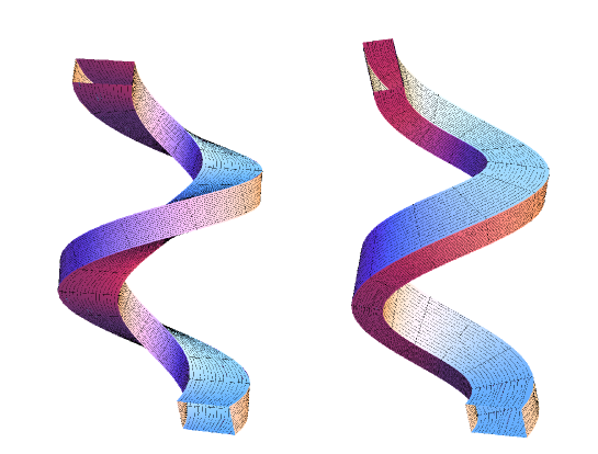
In Figure 3 we can see how the pair of Frenet normal vectors $\{N,B\}$ versus relatively parallel normal vectors $\{M_{1},M_{2}\}$ move along a helix. The longer side of the rectangular cross-section corresponds to the direction of $N$ (on the left) and $M_{1}$ (on the right), whereas the shorter side is the direction of $B$ and $M_{2}$, respectively. In the bottom of the Figure, the two frames coincide.

Figure 3: A waveguide with rectangular cross-section built along a helix. In the left figure the cross-section moves according to the Frenet frame, i.e. $\dot{\theta}_{F}=0$, so that the waveguide is twisted because $\dot{\theta}=-\tau\not=0$. In the right figure the cross section moves according to the RPAF, i.e. $\dot{\theta}=0$; we say that such a waveguide is untwisted.

Remark 3.2.

In Assumption 2 of Theorem 2.1, we state some requirements on the curvature functions $k_{1},k_{2}$ that are not uniquely determined for the reference curve, as we have seen in this subsection. However, let us fix some particular RPAF with curvatures $k_{1}^{0},k_{2}^{0}$ and recall that the curvatures for different RPAFs are only the linear combination of $k_{1}^{0}$ and $k_{2}^{0}$. When we examine the condition (2.7), we easily find that if $k_{1}^{0},k_{2}^{0}$ satisfy it, then all their linear combinations do satisfy it as well (due to the triangle inequality in $L^{2}$). Hence there is no ambiguity in Theorem 2.1.

3.2 The geometry of the tube

As mentioned in Introduction, the tubes we consider in this paper are obtained by translating and rotating a two-dimensional cross-section along a spatial curve $\Gamma$. This definition can be formalized by means of the RPAF $\{T,M_{1},M_{2}\}$ found in the previous section.

The cross-section of our tube can be quite arbitrary. We only assume that $\omega$ is a bounded open connected subset of $\mathbb{R}^{2}$. The boundedness implies that the quantity

$$a:=\sup_{t\in\omega}|t|$$ (3.5)

is finite. We say that $\omega$ is circular if it is a disc or an annulus centered at the origin of $\mathbb{R}^{2}$ (with the usual convention of identifying open sets which differ on the set of zero capacity).

Given an angle function $\theta\in W_{\mathrm{loc}}^{1,\infty}(I)$, let us define a rotation matrix

$$\mathcal{R}^{\theta}=\left(\begin{array}[]{cc}\cos{\theta}&\sin{\theta}\\ -\sin{\theta}&\cos{\theta}\\ \end{array}\right).$$

Then we define a general moving frame $\{M_{1}^{\theta},M_{2}^{\theta}\}$ along $\Gamma$ by rotating the RPAF $\{M_{1},M_{2}\}$ by the angle $\theta$, i.e.,

$$M_{\mu}^{\theta}=\sum_{\nu=1}^{2}\mathcal{R}^{\theta}_{\mu\nu}M_{\nu}\,,\qquad\mu=1,2\,.$$

Let $\Omega_{0}:=I\times\omega$ be a straight tube. We introduce a curved tube $\Omega_{\varepsilon}$ of uniform cross-section $\varepsilon\omega$ as the image

$$\Omega_{\varepsilon}:=\mathcal{L}(\Omega_{0})\,,$$ (3.6)

where the mapping $\mathcal{L}:$ $\Omega_{0}\rightarrow\mathbb{R}^{3}$ is defined by

$$\mathcal{L}(s,t):=\Gamma(s)+\varepsilon\sum_{\mu=1}^{2}t_{\mu}M_{\mu}^{\theta}\,.$$ (3.7)

We say that the tube $\Omega_{\varepsilon}$ is bent if the reference curve $\Gamma$ is not a straight line, i.e. $\kappa\not=0$. We say that $\Omega_{\varepsilon}$ is untwisted if $\omega$ is circular or the cross-section is moved along $\Gamma$ by a RPAF, i.e. $\dot{\theta}=0$; otherwise the tube is said to be twisted (for example of twisted and untwisted tube see Figure 3). A list of equivalent conditions for twisting can be found in [17].

It is usual in the theory of quantum waveguides to assume the tube $\Omega_{\varepsilon}$ is non-self-intersecting, i.e., $\mathcal{L}$ is injective. The necessary (but not always sufficient) condition for the injectivity is the non-vanishing determinant of the metric tensor

$$G_{ij}:=\partial_{i}\mathcal{L}\cdot\partial_{j}\mathcal{L}.$$

Here $\partial_{i}$ denotes the partial derivative with respect to the $i^{th}$ variable, where the ordered set ($s$, $t_{1}$, $t_{2}$) corresponds to (1,2,3). Employing (3.2), it is straightforward to check that the matrix $G=(G_{ij})$ reads

$$G=\left(\begin{array}[]{ccc}h^{2}+\varepsilon^{2}(h_{2}^{2}+h_{3}^{2})&-\varepsilon^{2}h_{3}&-\varepsilon^{2}h_{2}\\ -\varepsilon^{2}h_{3}&\varepsilon^{2}&0\\ -\varepsilon^{2}h_{2}&0&\varepsilon^{2}\\ \end{array}\right),$$ (3.8)

where

$$h(\cdot,t) :=1-\varepsilon\,t_{1}\left(k_{1}\cos{\theta}+k_{2}\sin{\theta}\right)-\varepsilon\,t_{2}\left(-k_{1}\sin{\theta}+k_{2}\cos{\theta}\right),$$ (3.9)

$$h_{2}(\cdot,t) :=-t_{1}\,\dot{\theta},$$

$$h_{3}(\cdot,t) :=t_{2}\,\dot{\theta}.$$

We have

$$|G|:=\det(G)=\varepsilon^{4}\;\!h^{2}\,,$$ (3.10)

hence the condition on the determinant being everywhere nonzero requires that $h$ is a positive function. The latter can be satisfied only if the functions $k_{1},k_{2}$ are bounded. Therefore we always assume

$$\kappa\in L^{\infty}(I)\,,$$ (3.11)

which is equivalent to the boundedness of $k_{1},k_{2}$ due to (3.3). In particular, we have

$$\|k_{\mu}\|_{\infty}\leq\|\kappa\|_{\infty}<\infty,\qquad\mu=1,2,$$ (3.12)

where $\|\cdot\|_{\infty}:=\|\cdot\|_{L^{\infty}(I)}$. Using in addition the boundedness of $\omega$, we find the bound

$$h(s,t)\geq 1-\varepsilon\;\!a\;\!\|\kappa\|_{\infty}$$ (3.13)

for every $(s,t)\in\Omega_{0}$. This ensures the positivity of $h$ for all sufficiently small $\varepsilon$.

If the determinant (3.10) is positive, the matrix (3.8) is invertible and we have

$$G^{-1}=\frac{1}{h^{2}}\begin{pmatrix}1&h_{3}&h_{2}\\ h_{3}&\varepsilon^{-2}h^{2}+h_{3}^{2}&h_{2}h_{3}\\ h_{2}&h_{3}h_{2}&\varepsilon^{-2}h^{2}+h_{2}^{2}\\ \end{pmatrix}.$$

Summing up, assuming (3.11) and the injectivity of $\mathcal{L}$, the mapping induces a global diffeomorphism between the straight tube $\Omega_{0}$ and $\Omega_{\varepsilon}$, and the latter has the usual meaning of a non-self-intersecting curved tube embedded in $\mathbb{R}^{3}$. For sufficient conditions ensuring the injectivity of $\mathcal{L}$ we refer to [10, App. A]. The above construction gives rise to Assumption 1.

Remark 3.3.

Abandoning the geometrical interpretation of $\Omega_{\varepsilon}$ being a non-self-intersecting tube in $\mathbb{R}^{3}$, it is possible to consider $(\Omega_{0},G)$ as an abstract Riemannian manifold, not necessarily embedded in $\mathbb{R}^{3}$. This makes (3.11) (together with the smallness of $\varepsilon$ to ensure that the right hand side of (3.13) is positive) the only important hypothesis in the present study. In other words, the injectivity assumption (iii) in Assumption 1 can be relaxed, the results of the present paper hold in this more general situation.

3.3 The Hamiltonian

Let us now consider $\Omega_{\varepsilon}$ as the configuration space of a quantum waveguide. We assume that the motion of a quantum particle inside the waveguide is effectively free and that the particle wavefunction is suppressed on the boundary of the tube. Hence, setting $\hbar=2m=1$, the one-particle Hamiltonian acts as the Laplacian on $L^{2}(\Omega_{\varepsilon})$ subjected to Dirichlet boundary conditions on $\partial\Omega_{\varepsilon}$:

$$-\Delta^{\Omega_{\varepsilon}}_{D}.$$ (3.14)

The objective of this subsection is to give a precise meaning to this operator.

The most straightforward way is to assume that $\mathcal{L}$ is injective and define (3.14) as the Dirichlet Laplacian on $L^{2}(\Omega_{\varepsilon})$. Indeed, this is well defined for open sets and from the previous subsection we know that $\mathcal{L}$ induces a global diffeomorphism, so that, in particular, $\Omega_{\varepsilon}$ is open. More specifically, the Dirichlet Laplacian $-\Delta^{\Omega_{\varepsilon}}_{D}$ is introduced as the self-adjoint operator associated on $L^{2}(\Omega_{\varepsilon})$ with the closed quadratic form

$$Q_{D}^{\Omega_{\varepsilon}}[\psi]:=\|\nabla\psi\|^{2}_{L^{2}(\Omega_{\varepsilon})}\,,\qquad\mathrm{Dom}\,(Q_{D}^{\Omega_{\varepsilon}})=W^{1,2}_{0}(\Omega_{\varepsilon}).$$

From this point of view, we regard the tube as a submanifold of $\mathbb{R}^{3}$. For the description of $\Omega_{\varepsilon}$, the most suitable coordinates are the curvilinear ‘coordinates’ $(s,t)\in\Omega_{0}$ defined via the mapping $\mathcal{L}$ in (3.7). They are implemented by means of the unitary transform

$$U_{1}:L^{2}(\Omega_{\varepsilon})\to\tilde{\mathcal{H}}_{\varepsilon}:=L^{2}\big{(}\Omega_{0},|G(s,t)|^{1/2}\;\!ds\;\!dt\big{)}:\big{\{}\psi\mapsto\psi\circ\mathcal{L}\big{\}}$$ (3.15)

mentioned already in (2.1). The transformed operator $\tilde{H}_{\varepsilon}:=U_{1}(-\Delta^{\Omega_{\varepsilon}}_{D})U_{1}^{-1}$ can be determined as the operator associated with the transformed form

$$\tilde{Q}_{\varepsilon}[\psi]:=Q_{D}^{\Omega_{\varepsilon}}[U_{1}^{-1}\psi]=\left(\partial_{i}\psi,G^{ij}\partial_{j}\psi\right)_{\tilde{\mathcal{H}}_{\varepsilon}}\,,\qquad\mathrm{Dom}\,(\tilde{Q}_{\varepsilon}):=U_{1}W^{1,2}_{0}(\Omega_{\varepsilon})\,.$$ (3.16)

Here $G^{ij}$ are coefficients of the inverse metric (3.8) and the Einstein summation convention is adopted (the range of indices $i,j$ being $1,2,3$). In a weak sense, $\tilde{H}_{\varepsilon}$ acts as the Laplace-Beltrami operator $-|G|^{-1/2}\partial_{i}|G|^{1/2}G^{ij}\partial_{j}$, but we shall not need this fact, working exclusively with quadratic forms in this paper.

Let us emphasize that, for the quadratic form $\tilde{Q}_{\varepsilon}$ to be well defined, the matrix $G$ does not need to be differentiable, a local boundedness of its elements is sufficient. As a matter of fact, the form domain $U_{1}W^{1,2}_{0}(\Omega_{0})$ can be alternatively characterized as the completion of $C_{0}^{\infty}(\Omega_{0})$ with respect to the norm

$$\|\psi\|_{\tilde{Q}_{\varepsilon}}:=\sqrt{\left(\partial_{i}\psi,G^{ij}\partial_{j}\psi\right)_{\tilde{\mathcal{H}}_{\varepsilon}}+\|\psi\|_{\tilde{\mathcal{H}}_{\varepsilon}}^{2}}\,.$$

If the functions $\kappa$ and $\dot{\theta}$ are bounded, it is possible to check that the $\tilde{Q}_{\varepsilon}$-norm is equivalent to the usual norm in $W^{1,2}(\Omega_{0})$. For this reason, in addition to (3.11), we assume henceforth the global boundedness

$$\dot{\theta}\in L^{\infty}(I)\,.$$ (3.17)

Then we have

$$\mathrm{Dom}\,(\tilde{Q}_{\varepsilon})=W^{1,2}_{0}(\Omega_{0})\,.$$ (3.18)

Remark 3.4.

Now, if $\mathcal{L}$ is not injective, the image (3.6) might be quite complex and the standard notion of the Dirichlet Laplacian on $\Omega_{\varepsilon}$ meaningless. Nevertheless, the Laplace-Beltrami operator on the Riemannian manifold $(\Omega_{0},G)$, i.e. the operator associated on $\tilde{\mathcal{H}}_{\varepsilon}$ with the closure of the form defined via the second identity in (3.16) on the initial domain $C_{0}^{\infty}(\Omega_{0})$, is fully meaningful. Moreover, it coincides with $\tilde{H}_{\varepsilon}$ defined above. This is the way how to transfer the results of the present paper to the more general situation of Remark 3.3. In particular, Theorem 2.1 holds without the injectivity assumption (iii) in Assumption 1 provided that we properly reinterpret the meaning of (3.14) as the Laplace-Beltrami operator $\tilde{H}_{\varepsilon}$ in $(\Omega_{0},G)$ and we write just $U_{2}$ instead of $U$ in the statement of the theorem when dealing with the more general situation.

Finally, let us recall that the spectrum of $\tilde{H}_{\varepsilon}$ explodes as $\varepsilon^{-2}E_{1}$ in the limit as $\varepsilon\to 0$. This is related to the fact that the ground-state eigenvalue of the cross-sectional Laplacian $-\Delta_{D}^{\varepsilon\omega}$ equals $\varepsilon^{-2}E_{1}$. Therefore, to get a non-trivial limit, we rather consider the renormalized operator

$$\tilde{\tilde{H}}_{\varepsilon}:=\tilde{H}_{\varepsilon}-\varepsilon^{-2}E_{1}$$

in the sequel.

4 The mollification strategy

Our strategy how to reduce the regularity assumptions about the waveguide consists of the three points (I)–(III) roughly mentioned in Section 2. The first of them, i.e. the usage of RPAF instead of the Frenet frame, was already explained in Section 3.1. The item (II) consists in working with associated sesquilinear forms instead of operators. In the preceding Section 3.3, we introduced the Dirichlet Laplacian in the tube $\Omega_{\varepsilon}$ using exclusively quadratic forms and it enables us to understand the derivatives in the weak sense and to reduce the requirements on the differentiability of the reference curve.

However, as explained in Section 2, for the standard operator procedure to work, certain additional smoothness of curvature functions are still needed. In this section we propose a method how to proceed without any extra regularity hypotheses. It is based on the mollification procedure (III) sketched in Section 2 and we believe it might be useful in other problems as well.

4.1 The modified unitary transform

As explained in Section 2, the main idea consists in mollifying the curvatures $k_{1},k_{2}$ by means of the Steklov approximation to get $k_{1}^{\varepsilon},k_{2}^{\varepsilon}$ introduced in (2.5). If $I$ is finite or semi-infinite, we adopt the convention of Assumption 2 to give a meaning to function values outside $I$ in the definition. That is, we assume that $k_{\mu}$, with $\mu=1,2$, are extended from $I$ to $\mathbb{R}$ by zero.

The definition (2.5) involves a positive continuous function $\varepsilon\mapsto\delta(\varepsilon)$ which is supposed to satisfy

$$\lim_{\varepsilon\rightarrow 0}\delta(\varepsilon)=0\qquad\textrm{and}\qquad\lim_{\varepsilon\rightarrow 0}\frac{\varepsilon}{\delta(\varepsilon)}=0.$$ (4.1)

Here the first assumption is reasonable since then $k_{\mu}^{\varepsilon}\xrightarrow[]{\varepsilon\rightarrow 0}k_{\mu}$ in a certain sense (see Section 4.2 below). The relevance of the second condition will become clear in our computations.

It follows from (3.3) that

$$\|k_{\mu}^{\varepsilon}\|_{\infty}\leq\|\kappa\|_{\infty},\qquad{\mu}=1,2.$$ (4.2)

Furthermore, the mollified functions are differentiable for any positive $\varepsilon$,

$$\dot{k}^{\varepsilon}_{\mu}(s)=\frac{k_{\mu}(s+\frac{\delta(\varepsilon)}{2})-k_{\mu}(s-\frac{\delta(\varepsilon)}{2})}{\delta(\varepsilon)},\qquad{\mu}=1,2,$$ (4.3)

although the derivative might diverge in the limit as $\varepsilon\to 0$ for non-differentiable functions $k_{\mu}$.

We also introduce a smoothed version of the ‘Jacobian’ (3.9)

$$h_{\varepsilon}(\cdot,t):=1-\varepsilon\,t_{1}\left(k^{\varepsilon}_{1}\cos{\theta}+k^{\varepsilon}_{2}\sin{\theta}\right)-\varepsilon\,t_{2}\left(-k^{\varepsilon}_{1}\sin{\theta}+k^{\varepsilon}_{2}\cos{\theta}\right)$$

and of the determinant (3.10), $|\tilde{G}|:=\varepsilon^{4}h_{\varepsilon}^{2}$. The latter will be used to generate a modified version of the standard unitary transform $U_{2}$ from Section 2. We define

$$\tilde{U}_{2}:\tilde{\mathcal{H}}_{\varepsilon}\to\mathcal{H}_{\varepsilon}:=L^{2}\left(\Omega_{0},\frac{|G(s,t)|^{1/2}}{|\tilde{G}(s,t)|^{1/2}}\,ds\,dt\right):\left\{\psi\mapsto|\tilde{G}|^{1/4}\psi\right\}.$$ (4.4)

The norm and inner product in the Hilbert space $\mathcal{H}_{\varepsilon}$ will be denoted by $\|\cdot\|_{\varepsilon}$ and $(\cdot,\cdot)_{\varepsilon}$, respectively.

In addition to (3.11), let us assume (3.17) in the following, so that the form domain of $\tilde{H}$ is given by (3.18). Since the Sobolev space $W_{0}^{1,2}(\Omega_{0})$ is left invariant by the modified transform $\tilde{U}_{2}$, the operator

$$H_{\varepsilon}:=\tilde{U}_{2}\tilde{\tilde{H}}_{\varepsilon}\tilde{U}_{2}^{-1}=|\tilde{G}|^{1/4}\tilde{\tilde{H}}_{\varepsilon}|\tilde{G}|^{-1/4}$$ (4.5)

is well defined in the form sense. The associated quadratic form reads

$$Q_{\varepsilon}[\psi]= \int_{\Omega_{0}}\frac{1}{hh_{\varepsilon}}\left|(\partial_{s}+\dot{\theta}\partial_{\alpha})\psi\right|^{2}\,ds\,dt+\frac{1}{\varepsilon^{2}}\int_{\Omega_{0}}\frac{h}{h_{\varepsilon}}|\nabla^{\prime}\psi|^{2}\,ds\,dt-\frac{E_{1}}{\varepsilon^{2}}\int_{\Omega_{0}}\frac{h}{h_{\varepsilon}}|\psi|^{2}\,ds\,dt$$ (4.6)

$$+\,\frac{1}{2}\int_{\Omega_{0}}\frac{1}{h_{\varepsilon}^{2}}(k_{1}k^{\varepsilon}_{1}+k_{2}k^{\varepsilon}_{2})|\psi|^{2}\,ds\,dt-\frac{3}{4}\int_{\Omega_{0}}\frac{h}{h_{\varepsilon}^{3}}\left((k^{\varepsilon}_{1})^{2}+(k^{\varepsilon}_{2})^{2}\right)|\psi|^{2}\,ds\,dt$$

$$+\int_{\Omega_{0}}\frac{\left((\partial_{s}+\dot{\theta}\partial_{\alpha})h_{\varepsilon}\right)^{2}}{4hh_{\varepsilon}^{3}}|\psi|^{2}\,ds\,dt-\int_{\Omega_{0}}\frac{(\partial_{s}+\dot{\theta}\partial_{\alpha})h_{\varepsilon}}{hh_{\varepsilon}^{2}}\,\mathrm{Re}(\bar{\psi}(\partial_{s}+\dot{\theta}\partial_{\alpha})\psi)\,ds\,dt,$$

with $\psi\in\mathrm{Dom}\,(Q_{\varepsilon})=W_{0}^{1,2}(\Omega_{0})$. Here $\nabla^{\prime}$ is the gradient operator in the ‘transverse’ variables $(t_{1},t_{2})$ and $\partial_{\alpha}$ is the transverse angular-derivative operator

$$\partial_{\alpha}:=(t_{2},-t_{1})\cdot\nabla^{\prime}=t_{2}\frac{\partial}{\partial t_{1}}-t_{1}\frac{\partial}{\partial t_{2}}\,.$$

An important feature of the operator $H_{\varepsilon}$ is its boundedness from below. We prove it together with another relation used in our computations below.

Lemma 4.1.

Let $Q_{\varepsilon}$ be the quadratic form defined by (4.6) and let (4.1) be satisfied. Then for all $\psi\in W^{1,2}_{0}(\Omega_{0})$ and small enough $\varepsilon$

$$Q_{\varepsilon}[\psi]\geq\frac{1}{2}\int_{\Omega_{0}}\frac{1}{hh_{\varepsilon}}\left|(\partial_{s}+\dot{\theta}\partial_{\alpha})\psi\right|^{2}\,ds\,dt-9\|\kappa\|_{\infty}^{2}\|\psi\|^{2}_{\varepsilon}.$$ (4.7)

Proof.

If we assume that $\varepsilon$ is so small that

$$\frac{3}{4}\leq 1-\varepsilon a\|\kappa\|_{\infty}\leq h\leq 1+\varepsilon a\|\kappa\|_{\infty}\leq\frac{5}{4}\,,$$

then the same relation holds for $h_{\varepsilon}$ and using (3.12) we easily get

$$\left|\frac{1}{2}\int_{\Omega_{0}}\frac{1}{h_{\varepsilon}^{2}}(k_{1}k^{\varepsilon}_{1}+k_{2}k^{\varepsilon}_{2})|\psi|^{2}\,ds\,dt-\frac{3}{4}\int_{\Omega_{0}}\frac{h}{h_{\varepsilon}^{3}}\left((k^{\varepsilon}_{1})^{2}+(k^{\varepsilon}_{2})^{2}\right)|\psi|^{2}\,ds\,dt\right|\leq 5\|\kappa\|_{\infty}^{2}\|\psi\|_{\varepsilon}^{2}.$$

The estimate on terms proportional to $\varepsilon^{-2}$ is based on the Poincaré-type inequality

$$\int_{\omega}|\nabla^{\prime}\phi|^{2}dt-E_{1}\int_{\omega}|\phi|^{2}dt\geq 0$$

that holds for all $\phi\in W^{1,2}_{0}(\omega)$, and on Fubini’s theorem. Due to nontrivial measure in our integrals, we have to use substitution $\phi:=\sqrt{h/h_{\varepsilon}}\;\!\psi$, then we obtain

$$\frac{1}{\varepsilon^{2}}\int_{\Omega_{0}}\frac{h}{h_{\varepsilon}}|\nabla^{\prime}\psi|^{2}\,ds\,dt-\frac{E_{1}}{\varepsilon^{2}}\int_{\Omega_{0}}\frac{h}{h_{\varepsilon}}|\psi|^{2}\,ds\,dt$$

$$=\frac{1}{\varepsilon^{2}}\int_{\Omega_{0}}\left(|\nabla^{\prime}\phi|^{2}-E_{1}|\phi|^{2}\right)\,ds\,dt$$

$$\phantom{=}+\int_{\Omega_{0}}\left(\frac{3(k_{1}^{2}+k_{2}^{2})}{4h^{2}}-\frac{k_{1}k^{\varepsilon}_{1}+k_{2}k^{\varepsilon}_{2}}{2hh_{\varepsilon}}-\frac{(k^{\varepsilon}_{1})^{2}+(k^{\varepsilon}_{2})^{2}}{4h_{\varepsilon}^{2}}\right)|\phi|^{2}\,ds\,dt$$

$$\geq-3\|\kappa\|_{\infty}^{2}\int_{\Omega_{0}}|\phi|^{2}\,ds\,dt=-3\|\kappa\|_{\infty}^{2}\|\psi\|^{2}_{\varepsilon}.$$

The last term in (4.6) can be estimated using the Schwarz inequality and the simple Young’s inequality ($2ab\leq a^{2}+b^{2}$)

$$\left|\int_{\Omega_{0}}\frac{(\partial_{s}+\dot{\theta}\partial_{\alpha})h_{\varepsilon}}{hh_{\varepsilon}^{2}}\,\mathrm{Re}(\bar{\psi}(\partial_{s}+\dot{\theta}\partial_{\alpha})\psi)\,ds\,dt\right|\\ \leq\frac{1}{2}\left[\int_{\Omega_{0}}\frac{\left((\partial_{s}+\dot{\theta}\partial_{\alpha})h_{\varepsilon}\right)^{2}}{4hh_{\varepsilon}^{3}}|\psi|^{2}\,ds\,dt+\int_{\Omega_{0}}\frac{1}{hh_{\varepsilon}}\left|(\partial_{s}+\dot{\theta}\partial_{\alpha})\psi\right|^{2}\,ds\,dt\right].$$ (4.8)

Summing up, we get

$$Q_{\varepsilon}[\psi]\geq\frac{1}{2}\int_{\Omega_{0}}\frac{1}{hh_{\varepsilon}}\left|(\partial_{s}+\dot{\theta}\partial_{\alpha})\psi\right|^{2}\,ds\,dt-8\|\kappa\|_{\infty}^{2}\|\psi\|^{2}_{\varepsilon}-\int_{\Omega_{0}}\frac{\left((\partial_{s}+\dot{\theta}\partial_{\alpha})h_{\varepsilon}\right)^{2}}{4hh_{\varepsilon}^{3}}|\psi|^{2}\,ds\,dt$$

and the proof is finished by the estimate

$$\left|\int_{\Omega_{0}}\frac{\left((\partial_{s}+\dot{\theta}\partial_{\alpha})h_{\varepsilon}\right)^{2}}{4hh_{\varepsilon}^{3}}|\psi|^{2}\,ds\,dt\right|\leq 51\frac{\varepsilon^{2}}{\delta(\varepsilon)^{2}}a^{2}\|\kappa\|_{\infty}^{2}\|\psi\|^{2}_{\varepsilon}\leq\|\kappa\|_{\infty}^{2}\|\psi\|^{2}_{\varepsilon}$$

which holds for small enough $\varepsilon$ due to (4.1). ∎

As a consequence of Lemma 4.1, we get that for a constant $\lambda<-9\|\kappa\|_{\infty}$ the operator $H_{\varepsilon}-\lambda$ is invertible and it holds

$$\|(H_{\varepsilon}-\lambda)^{-1}\|_{\mathcal{B}(H_{\varepsilon})}\leq\frac{1}{|\lambda|-9\|\kappa\|_{\infty}^{2}}\,.$$ (4.9)

4.2 Convergence properties of the Steklov approximation

Let $f$ be a bounded function defined on an interval $I$ and let $f^{\varepsilon}$ be its Steklov approximation

$$f^{\varepsilon}(s):=\frac{1}{\delta(\varepsilon)}\int_{s-\frac{\delta(\varepsilon)}{2}}^{s+\frac{\delta(\varepsilon)}{2}}f(\xi)\,d\xi$$ (4.10)

where $\delta$ is a positive continuous function on $\mathbb{R}$ satisfying the first of the requirements of (4.1). Again, we recall the extension convention of Assumption 2 if $I$ is finite or semi-infinite.

In the computations below we require for $f=k_{1},k_{2},\dot{\theta}$ that in a certain sense $f^{\varepsilon}$ converges to $f$ in the limit $\varepsilon\to 0$. Namely, the crucial requirement reads

$$\left(\int_{I}\left|f-f^{\varepsilon}\right|^{2}|\varphi|^{2}ds\right)^{1/2}\xrightarrow{\varepsilon\rightarrow 0}0\,,\qquad\forall\varphi\in W^{1,2}_{0}(I).$$ (4.11)

In the following we will find the requirements on $f$ such that this condition is satisfied.

We shall start with the estimate on the left hand side of (4.11).

Lemma 4.2.

Let $f\in L^{\infty}(I)$ and let $f^{\varepsilon}$ be the Steklov approximation of $f$. Let $\varphi\in W^{1,2}(I)$ and finally let $\{a_{n}\}_{n=n_{-}}^{n_{+}}\subset I$, $n\in\mathbb{Z}$ be the strictly increasing sequence of numbers where $a_{n_{-}}=\inf_{s\in I}s$, $a_{n_{+}}=\sup_{s\in I}s$, all the intervals $I_{n}:=(a_{n},a_{n+1})$ are finite and $n_{\pm}$ can be either finite number or $\pm\infty$. Then

$$\int_{I}\left|f-f^{\varepsilon}\right|^{2}|\varphi|^{2}ds\leq\sup_{n_{-}\leq n\leq n_{+}}\left[\left(\frac{\|f-f^{\varepsilon}\|^{2}_{L^{2}(I_{n})}}{a_{n+1}-a_{n}}\right)+2\|f-f^{\varepsilon}\|^{2}_{L^{2}(I_{n})}\right]\|\varphi\|^{2}_{W^{1,2}(I)}.$$ (4.12)

Proof.

The main idea of the proof is rewriting the estimated expression as

$$\int_{I}|f-f^{\varepsilon}|^{2}|\varphi|^{2}ds=\sum_{n=n_{-}}^{n_{+}-1}\int_{a_{n}}^{a_{n+1}}\dot{g}_{\varepsilon}^{n}|\varphi|^{2}ds=\sum_{n=n_{-}}^{n_{+}-1}\left(\left[{g}_{\varepsilon}^{n}|\varphi|^{2}\right]_{a_{n}}^{a_{n+1}}-\int_{a_{n}}^{a_{n+1}}g_{\varepsilon}^{n}\,2\mathrm{Re}\left(\bar{\varphi}\dot{\varphi}\right)ds\right)$$

where we integrated by parts and where we defined, for all $s\in I$,

$$g_{\varepsilon}^{n}(s):=\int_{a_{n}}^{s}|f(\xi)-f^{\varepsilon}(\xi)|^{2}\chi_{n}(\xi)d\xi,$$

$\chi_{n}(\xi)$ is the characteristic function of the interval $I_{n}$ (i.e., $\chi_{n}(\xi)=1$ for $\xi\in[a_{n},a_{n+1}]$ and $\chi_{n}(\xi)=0$ elsewhere). The proof is then completed by using the Schwarz and Young inequalities and the relations

$$\sup_{s\in I}g_{\varepsilon}^{n}(s) =g_{\varepsilon}^{n}(a_{n+1})=\int_{a_{n}}^{a_{n+1}}|f(\xi)-f^{\varepsilon}(\xi)|^{2}d\xi=\|f-f^{\varepsilon}\|^{2}_{L^{2}(I_{n})},$$

$$|\varphi(a_{n+1})|^{2} \leq\left(\frac{1}{a_{n+1}-a_{n}}+1\right)\|\varphi\|_{W^{1,2}(I_{n})}.$$

∎

The lemma is of great importance for our computations. From the generalized Minkowski inequality it follows that

$$\|f-f^{\varepsilon}\|_{L^{2}(I_{n})}\leq\sup_{|\eta|\leq\frac{\delta(\varepsilon)}{2}}\left(\int_{I_{n}}\left|f(s)-f(s+\eta)\right|^{2}ds\right)^{1/2}=:\omega_{2}(\delta(\varepsilon),f,I_{n}).$$ (4.13)

Here the notational symbol $\omega_{p}$ is adopted from [1], where it is referred to as modulus of continuity generalized to space $L^{p}$ and is computed for a function $f$, positive number $\delta(\varepsilon)$ and interval $I_{n}$. In [1] it is also shown that this quantity tends to zero with $\delta(\varepsilon)$ if the interval $I_{n}$ is finite. This directly yields that if the interval $I$ is finite, the convergence (4.11) holds.

If $I$ is infinite, we can cut it into finite intervals $(a_{n},a_{n+1})$ and for each $n$ the expression in square brackets on the right hand side of (4.12) would tend to zero when $\varepsilon\rightarrow 0$. Unfortunately, the supremum over $n_{-}\leq n\leq n_{+}$ might not have the zero limit. On the other hand, this may happen only in a case of functions that oscillate quickly at infinity (see Example 6.2). In other words, also for unbounded $I$, the condition (4.11) is satisfied for functions that behave ‘reasonably’ at infinity.

We summarize the above ideas in the following proposition. For simplicity, we use the result of Lemma 4.2 for the equidistant division $a_{n}:=n$ and we recall the extension convention of Assumption 2 for finite or semi-infinite $I$.

Proposition 4.3.

Let $\varphi\in W^{1,2}_{0}(I)$, $f\in L^{\infty}(I)$ and let $f^{\varepsilon}$ be the Steklov approximation of $f$ given by (4.10). Then

$$\left(\int_{I}\left|f-f^{\varepsilon}\right|^{2}|\varphi|^{2}ds\right)^{1/2}\leq\sqrt{3}\ \sigma_{f}(\delta(\varepsilon))\,\|\varphi\|_{W^{1,2}(I)}$$ (4.14)

where $\sigma_{f}(\delta(\varepsilon))$ is given by (2.6). Furthermore, the quantity $\sigma_{f}(\delta(\varepsilon))$ tends to zero as $\varepsilon\to 0$ if any of the following conditions is satisfied:

• $I$ is finite,

• $f$ periodic on $I_{\mathrm{ext}}$,

• $f\in L^{2}(I_{\mathrm{ext}})$,

• $f\in C^{0}(\overline{I_{\mathrm{ext}}})$,

where $I_{\mathrm{ext}}:=I\setminus\overline{I_{\mathrm{int}}}$ for some finite open (possibly empty) interval $I_{\mathrm{int}}$.

Proof.

The inequality (4.14) follows from Lemma 4.2 and the relation (4.13). It reminds to prove the convergence properties of (2.6).

Any bounded interval $I$ can be covered by intervals $I_{n}=(n,n+1]$, $n\in\mathcal{I}$ with $\mathcal{I}\subset\mathbb{Z}$ finite. Then $\sigma_{f}(\delta(\varepsilon))$ is proportional to maximum of $\omega_{2}(\delta(\varepsilon),f,I_{n})$ over $n\in\mathcal{I}$. Since $\omega_{2}(\delta(\varepsilon),f,I_{n})$ converges to zero for every $n\in\mathcal{I}$ as we explained above, $\sigma_{f}(\delta(\varepsilon))$ converges to zero if interval $I$ is finite. For the same reason the convergence of $\sigma_{f}(\delta(\varepsilon))$ does not depend on the behaviour of $f$ on a bounded subinterval $I_{\mathrm{int}}\subset I$ in case of infinite or semi-infinite $I$ .

Also the convergence of $\sigma_{f}(\delta(\varepsilon))$ for periodic functions follows from the fact that the period of length $q<\infty$ can be covered by finite number of intervals $(n,n+1]$. (More straightforwardly, using the sequence $a_{n}=nq$ in Lemma 4.2, we get $\sigma_{f}(\delta(\varepsilon))\propto\omega_{2}(\delta(\varepsilon),f,(0,q))$, which tends to zero as $\varepsilon\to 0$.)

In the case of $L^{2}$-functions, we use the fact that for any $\varepsilon>0$ there exists a finite interval $I_{\mathrm{int}}$ such that $f(s)<\varepsilon$ for all $s\in\mathbb{R}\setminus I_{\mathrm{int}}$. Then again the significant contribution to $\sigma_{f}(\delta(\varepsilon))$ comes from the finite interval.

Finally, for the uniformly continuous functions the situation is even more simple. Here already the quantity

$$\omega_{\infty}(\delta(\varepsilon),f):=\sup_{|\xi_{1}-\xi_{2}|\leq\delta(\varepsilon)}\left|f(\xi_{1})-f(\xi_{2})\right|\qquad\xi_{1},\xi_{2}\in I_{\mathrm{ext}},$$

called the modulus of continuity in [1], tends to zero when $\delta(\varepsilon)$ tends to zero and $\sigma_{f}(\delta(\varepsilon))$ can be estimated by $\omega_{\infty}(\delta(\varepsilon),f)$. Let us note that if $I$ is bounded or semi-bounded, the function need not to be uniformly continuous after extension by zero outside $I$. However, the convergence can be still ensured by dividing $I$ on the $\delta(\varepsilon)$-neighbourhood of the end point(s) and the rest of $I$. Then we can estimate the integral over inner part by $\omega_{\infty}(\delta(\varepsilon),f)$ since here the function is indeed uniformly continuous, the remaining integral can be estimated by $\|f\|_{\infty}\delta(\varepsilon)$ which tends to zero as well. ∎

5 The norm-resolvent convergence

In this long and technically demanding section we give a proof of Theorem 2.1.

5.1 Comparing operators acting on different Hilbert spaces

We start with describing a way how to understand the resolvent convergence of operators $-\Delta_{D}^{\Omega_{\varepsilon}}$ and $H_{\mathrm{eff}}$ acting on different Hilbert spaces $L^{2}(\Omega_{\varepsilon})$ and $L^{2}(I)$, respectively.

First of all, we recall that, in Section 4.1, we introduced the operator $H_{\varepsilon}$ on $\mathcal{H}_{\varepsilon}$ which is unitarily equivalent to $-\Delta_{D}^{\Omega_{\varepsilon}}-\varepsilon^{-2}E_{1}$. It is therefore enough to explain the resolvent convergence of $H_{\varepsilon}$ and $H_{\mathrm{eff}}$. Our strategy is to reconsider these operators as certain operators on the fixed Hilbert space

$$\mathcal{H}_{0}:=L^{2}(\Omega_{0})$$

and to show that the error due to the replacement becomes negligible in the limit as $\varepsilon\to 0$.

Recall that we have denoted the norm and inner product in the $\varepsilon$-dependent Hilbert space $\mathcal{H}_{\varepsilon}$ by $\|\cdot\|_{\varepsilon}$ and $(\cdot,\cdot)_{\varepsilon}$, respectively. We simply write $\|\cdot\|$ and $(\cdot,\cdot)$ for the norm and inner product in $\mathcal{H}_{0}$. Finally, $\|\cdot\|_{I}$ and $(\cdot,\cdot)_{I}$ stand for the norm and inner product in $L^{2}(I)$.

In order to have a way to compare operators acting on $\mathcal{H}_{\varepsilon}$ and $\mathcal{H}_{0}$, let us introduce yet another unitary transform

$$U_{\varepsilon}:\mathcal{H}_{\varepsilon}\to\mathcal{H}_{0}:\left\{\psi\mapsto\frac{|G|^{1/4}}{|\tilde{G}|^{1/4}}\psi\right\}\,.$$ (5.1)

For the convenience of the reader, we present here the following diagram explaining the relation with the other unitary transforms introduced so far:

$$L^{2}(\Omega_{\varepsilon})\xrightarrow[]{\quad U_{1}\quad}\begin{aligned} \lx@xy@svg{\hbox{\raise 0.0pt\hbox{\kern 7.08347pt\hbox{\ignorespaces\ignorespaces\ignorespaces\hbox{\vtop{\kern 0.0pt\offinterlineskip\halign{\entry@#!@&&\entry@@#!@\cr&\\&\\&\crcr}}}\ignorespaces{\hbox{\kern-3.0pt\raise 0.0pt\hbox{\hbox{\kern 0.0pt\raise 0.0pt\hbox{\hbox{\kern 3.0pt\raise 0.0pt\hbox{$\textstyle{}$}}}}}}}{\hbox{\kern 31.08347pt\raise 0.0pt\hbox{\hbox{\kern 0.0pt\raise 0.0pt\hbox{\hbox{\kern 3.0pt\raise 0.0pt\hbox{$\textstyle{\mathcal{H}_{0}}$}}}}}}}{\hbox{\kern-7.08347pt\raise-38.53276pt\hbox{\hbox{\kern 0.0pt\raise 0.0pt\hbox{\hbox{\kern 3.0pt\raise 0.0pt\hbox{$\textstyle{\tilde{\mathcal{H}}_{\varepsilon}\ignorespaces\ignorespaces\ignorespaces\ignorespaces\ignorespaces\ignorespaces\ignorespaces\ignorespaces}$}}}}}}}\ignorespaces\ignorespaces\ignorespaces{}\ignorespaces\ignorespaces{\hbox{\lx@xy@drawline@}}\ignorespaces\ignorespaces\ignorespaces{\hbox{\kern 6.19315pt\raise-13.23029pt\hbox{{}\hbox{\kern 0.0pt\raise 0.0pt\hbox{\hbox{\kern 3.0pt\hbox{\hbox{\kern 0.0pt\raise-1.74722pt\hbox{$\scriptstyle{U_{2}}$}}}\kern 3.0pt}}}}}}\ignorespaces{\hbox{\kern 34.33989pt\raise-4.80444pt\hbox{\hbox{\kern 0.0pt\raise 0.0pt\hbox{\lx@xy@tip{1}\lx@xy@tip{-1}}}}}}\ignorespaces\ignorespaces{\hbox{\lx@xy@drawline@}}\ignorespaces{\hbox{\lx@xy@drawline@}}\ignorespaces\ignorespaces\ignorespaces{}\ignorespaces\ignorespaces{\hbox{\lx@xy@drawline@}}\ignorespaces\ignorespaces\ignorespaces{\hbox{\kern 6.23326pt\raise-64.90497pt\hbox{{}\hbox{\kern 0.0pt\raise 0.0pt\hbox{\hbox{\kern 3.0pt\hbox{\hbox{\kern 0.0pt\raise-2.96667pt\hbox{$\scriptstyle{\tilde{U}_{2}}$}}}\kern 3.0pt}}}}}}\ignorespaces{\hbox{\kern 31.17778pt\raise-68.92279pt\hbox{\hbox{\kern 0.0pt\raise 0.0pt\hbox{\lx@xy@tip{1}\lx@xy@tip{-1}}}}}}\ignorespaces\ignorespaces{\hbox{\lx@xy@drawline@}}\ignorespaces{\hbox{\lx@xy@drawline@}}{\hbox{\kern 36.23347pt\raise-38.53276pt\hbox{\hbox{\kern 0.0pt\raise 0.0pt\hbox{\hbox{\kern 3.0pt\raise 0.0pt\hbox{$\textstyle{}$}}}}}}}{\hbox{\kern-3.0pt\raise-76.76607pt\hbox{\hbox{\kern 0.0pt\raise 0.0pt\hbox{\hbox{\kern 3.0pt\raise 0.0pt\hbox{$\textstyle{}$}}}}}}}{\hbox{\kern 31.17778pt\raise-76.76607pt\hbox{\hbox{\kern 0.0pt\raise 0.0pt\hbox{\hbox{\kern 3.0pt\raise 0.0pt\hbox{$\textstyle{\mathcal{H}_{\varepsilon}\ignorespaces\ignorespaces\ignorespaces\ignorespaces}$}}}}}}}\ignorespaces\ignorespaces\ignorespaces\ignorespaces{}{\hbox{\lx@xy@droprule}}\ignorespaces\ignorespaces\ignorespaces{\hbox{\kern 39.23347pt\raise-38.38304pt\hbox{{}\hbox{\kern 0.0pt\raise 0.0pt\hbox{\hbox{\kern 3.0pt\hbox{\hbox{\kern 0.0pt\raise-1.9611pt\hbox{$\scriptstyle{U_{\varepsilon}}$}}}\kern 3.0pt}}}}}}\ignorespaces{\hbox{\kern 39.23347pt\raise-4.80444pt\hbox{\hbox{\kern 0.0pt\raise 0.0pt\hbox{\lx@xy@tip{1}\lx@xy@tip{-1}}}}}}{\hbox{\lx@xy@droprule}}{\hbox{\lx@xy@droprule}}\ignorespaces}}}}\ignorespaces\end{aligned} \textstyle{\mathcal{H}_{0}} \textstyle{\tilde{\mathcal{H}}_{\varepsilon}\ignorespaces\ignorespaces\ignorespaces\ignorespaces\ignorespaces\ignorespaces\ignorespaces\ignorespaces} \scriptstyle{U_{2}} \scriptstyle{\tilde{U}_{2}} \textstyle{\mathcal{H}_{\varepsilon}\ignorespaces\ignorespaces\ignorespaces\ignorespaces} \scriptstyle{U_{\varepsilon}}$$ (5.2)

It is important to emphasize that while the transformed resolvent $U_{\varepsilon}(H_{\varepsilon}-i)^{-1}U_{\varepsilon}^{-1}$ on $\mathcal{H}_{0}$ is well defined (as a unitary transform of a bounded operator), the similar expression for the (unbounded) operator $H_{\varepsilon}$ may not have any sense. Indeed, $H_{\varepsilon}$ acts as a differential operator, while $|G|$ may not be differentiable under our minimal assumption. The same remark applies to $\tilde{H}_{\varepsilon}$ and $U_{2}$, as already pointed out in Section 2.

Summing up, using the unitary transforms described above, it is possible to reconsider the resolvent of the Dirichlet Laplacian $-\Delta_{D}^{\Omega_{\varepsilon}}$ as an operator on $\mathcal{H}_{0}$. It remains to explain how to reconsider $H_{\mathrm{eff}}$ acting on $L^{2}(I)$ as an operator on the ‘larger’ space $\mathcal{H}_{0}$. This is done by introducing the following subspace of $\mathcal{H}_{0}$:

$$\mathcal{H}_{0}^{1}:=\left\{\psi\in\mathcal{H}_{0}\,\left|\right.\,\exists\varphi\in L^{2}(I),\,\psi(s,t)=\varphi(s)\mathcal{J}_{1}(t)\right\}.$$ (5.3)

Recall that $\mathcal{J}_{1}$ denotes the eigenfunction corresponding to first eigenvalue of the transverse Dirichlet Laplacian $-\Delta_{D}^{\omega}$; we choose it to be positive and normalized to one in $L^{2}(\omega)$. $\mathcal{H}_{0}^{1}$ is closed, hence

$$\mathcal{H}_{0}=\mathcal{H}_{0}^{1}\oplus(\mathcal{H}_{0}^{1})^{\bot}$$ (5.4)

and every function $\psi\in\mathcal{H}_{0}$ can be uniquely written as

$$\psi=P_{1}\psi+(1-P_{1})\psi=:\psi_{1}\mathcal{J}_{1}+\psi^{\bot}$$ (5.5)

with $\psi_{1}\mathcal{J}_{1}\in\mathcal{H}_{0}^{1}$, $\psi^{\bot}\in(\mathcal{H}_{0}^{1})^{\bot}$ and $P_{1}$ being projection on $\mathcal{H}_{0}^{1}$,

$$(P_{1}\psi)(s,t):=\left(\int_{\omega}\mathcal{J}_{1}(t)\psi(s,t)dt\right)\mathcal{J}_{1}(t)\equiv\psi_{1}(s)\mathcal{J}_{1}(t).$$ (5.6)

To shorten the notation, we denote by $\psi_{1}\mathcal{J}_{1}$ the function $\psi_{1}\otimes\mathcal{J}_{1}$, i.e. the function on $I\times\omega$ which assumes values as $\psi_{1}(s)\mathcal{J}_{1}(t)$. Such a decomposition of functions $\psi\in\mathcal{H}_{0}$ will be extensively used throughout the text with the same notation.

Now we can introduce the isometric isomorphism

$$\pi:\mathcal{H}_{0}^{1}\to L^{2}(I):\left\{\psi_{1}(s)\mathcal{J}_{1}(t)\mapsto\psi_{1}(s)\right\}\,.$$

Let $q_{\mathrm{eff}}$ be the quadratic form associated with the operator $H_{\mathrm{eff}}$, i.e.,

$$q_{\mathrm{eff}}[\varphi]=\int_{I}|\dot{\varphi}(s)|^{2}ds+C_{\omega}\int_{I}\dot{\theta}(s)^{2}|\varphi(s)|^{2}ds-\frac{1}{4}\int_{I}\kappa(s)^{2}|\varphi(s)|^{2}ds\,,\qquad\mathrm{Dom}\,(q_{\mathrm{eff}})=W_{0}^{1,2}(I)\,.$$

(Recall that the basic Assumption 1 requires that both $\kappa$ and $\dot{\theta}$ are bounded functions, so that $H_{\mathrm{eff}}$ is well defined as a bounded perturbation of the one-dimensional Dirichlet Laplacian $-\Delta_{D}^{I}$.) The form $q_{\mathrm{eff}}$ can be identified with the quadratic form $Q_{\mathrm{eff}}$ acting on the subspace $\mathcal{H}_{0}^{1}$ as

$$Q_{\mathrm{eff}}[\psi_{1}\mathcal{J}_{1}] :=\int_{\Omega_{0}}|\partial_{s}\psi_{1}\mathcal{J}_{1}|^{2}\,ds\,dt-\frac{1}{4}\int_{\Omega_{0}}\kappa^{2}|\psi_{1}\mathcal{J}_{1}|^{2}\,ds\,dt+C_{\omega}\int_{\Omega_{0}}\dot{\theta}^{2}|\psi_{1}\mathcal{J}_{1}|^{2}\,ds\,dt=q_{\mathrm{eff}}[\psi_{1}]\,,$$ (5.7)

$$\mathrm{Dom}\,(Q_{\mathrm{eff}}) :=\{\psi\in\mathcal{H}_{0}^{1}\,|\,\psi_{1}\in W_{0}^{1,2}(I)\}\,.$$

In a similar way we can identify operators acting on $\mathcal{H}_{0}^{1}\subset\mathcal{H}_{0}$ and $L^{2}(I)$. We tacitly employ the identification, without writing down the identification mapping $\pi$ explicitly in the formulae. In particular, denoting by $0^{\bot}$ the zero operator on $(\mathcal{H}_{0}^{1})^{\bot}$, the operator $\left(H_{\mathrm{eff}}-i\right)^{-1}\oplus 0^{\bot}$ can be understood as an operator acting on the whole space $\mathcal{H}_{0}$.

5.2 Proof of Theorem 2.1

At first let us explain the connection between the operator $U(-\Delta_{D}^{\Omega_{\varepsilon}}-\varepsilon^{-2}E_{1}-i)^{-1}U^{-1}$ from formula (2.10) and the operator $U_{\varepsilon}(H_{\varepsilon}-i)^{-1}U_{\varepsilon}^{-1}$ we spoke about in the previous section. More precisely, we show that these two operators are identical. Indeed, recall that $U=U_{2}U_{1}$ where $U_{1}$ and $U_{2}$ are unitary transforms described in Section 2 and in addition that $H_{\varepsilon}=\tilde{U}_{2}U_{1}(-\Delta_{D}^{\Omega_{\varepsilon}}-\varepsilon^{-2}E_{1})U_{1}^{-1}\tilde{U}_{2}^{-1}$. Using the diagram (5.2) we easily get that

$$U_{2}U_{1}(-\Delta_{D}^{\Omega_{\varepsilon}}-\varepsilon^{-2}E_{1}-i)^{-1}U_{1}^{-1}U_{2}^{-1}=U_{\varepsilon}\tilde{U}_{2}U_{1}(-\Delta_{D}^{\Omega_{\varepsilon}}-\varepsilon^{-2}E_{1}-i)^{-1}U_{1}^{-1}\tilde{U}_{2}^{-1}U_{\varepsilon}^{-1}=U_{\varepsilon}(H_{\varepsilon}-i)^{-1}U_{\varepsilon}^{-1}$$

and in following we will prove Theorem 2.1 using the last expression.

Another point is that according to [16] (Theorem IV.2.25), if the formula (2.10) is satisfied for a $\lambda$ from the resolvent set of $H_{\mathrm{eff}}$, then it holds true for all such $\lambda$. In particular there exists a constant $C_{\lambda}$ such that

$$\left\|U_{\varepsilon}(H_{\varepsilon}-i)^{-1}U_{\varepsilon}^{-1}-\left(\left(H_{\mathrm{eff}}-i\right)^{-1}\oplus 0^{\bot}\right)\right\|_{\mathcal{B}(\mathcal{H}_{0})}\\ \leq C_{\lambda}\left\|U_{\varepsilon}(H_{\varepsilon}-\lambda)^{-1}U_{\varepsilon}^{-1}-\left(\left(H_{\mathrm{eff}}-\lambda\right)^{-1}\oplus 0^{\bot}\right)\right\|_{\mathcal{B}(\mathcal{H}_{0})}.$$ (5.8)

Hence our aim is to prove that the right hand side of the last expression tends to zero for some $\lambda<-9\|\kappa\|_{\infty}^{2}$, since such $\lambda$ belongs to resolvent set of $H_{\mathrm{eff}}$ and also of $H_{\varepsilon}$ (cf (4.7) which yields $Q_{\varepsilon}[\psi]\geq-9\|\kappa\|_{\infty}^{2}\|\psi\|^{2}_{\varepsilon}$, similarly $q_{\mathrm{eff}}[\psi]\geq-\frac{1}{4}\|\kappa\|_{\infty}^{2}\|\psi\|_{I}^{2}$). This proof is divided into proof of two auxiliary lemmata, where in every lemma we compare one of the operators on the right hand side of (5.8) with the resolvent of operator

$$H_{0}:=1\otimes\left(-\frac{1}{\varepsilon^{2}}\Delta^{\omega}_{D}-\frac{E_{1}}{\varepsilon^{2}}\right)+\left(-\Delta^{I}_{D}-\frac{\kappa^{2}}{4}+C_{\omega}\dot{\theta}^{2}\right)\otimes 1.$$ (5.9)

The crucial step lies in comparison of $H_{0}$ and $H_{\varepsilon}$ stated in the first of these lemmata.

Lemma 5.1.

Let $\lambda<-9\|\kappa\|_{\infty}^{2}$ be a real constant and let the assumptions of Theorem 2.1 be satisfied. Then

$$\|U_{\varepsilon}(H_{\varepsilon}-\lambda)^{-1}U_{\varepsilon}^{-1}-(H_{0}-\lambda)^{-1}\|_{\mathcal{B}(\mathcal{H}_{0})}\leq\tilde{C}\left(\varepsilon+\varepsilon\left(\|\dot{k}^{\varepsilon}_{1}\|_{\infty}+\|\dot{k}^{\varepsilon}_{2}\|_{\infty}\right)+\sigma(\delta(\varepsilon))\right)$$ (5.10)

for some constant $\tilde{C}$.

Second lemma giving the comparison of $H_{0}$ and $H_{\mathrm{eff}}$ represents only a tiny improvement of the result above.

Lemma 5.2.

Let $H_{0}$ be the operator defined by (5.9) and let $H_{\mathrm{eff}}$ be the effective Hamiltonian (2.3). Then

$$\|\left(H_{0}-\lambda\right)^{-1}-\left(\left(H_{\mathrm{eff}}-\lambda\right)^{-1}\oplus 0^{\bot}\right)\|_{\mathcal{B}(\mathcal{H}_{0})}\leq\tilde{\tilde{C}}\varepsilon$$

for some real constants $\tilde{\tilde{C}}$ and $\lambda<-9\|\kappa\|_{\infty}^{2}$.

Proofs of Lemmata 5.1 and 5.2 will be given in Sections 5.4 and 5.3, respectively. These lemmata will be proved using a trick employed originally in [13], where the estimate on the norm of the difference of resolvents is obtained by a usage of the associated quadratic forms. We state the following proposition to give the reader basic idea of this trick; in our proofs we have to modify it due to distinctness of Hilbert spaces our operators act on and the main idea could be hidden by loads of technicalities.

Proposition 5.3.

Let $A,B$ be positive self-adjoint operators acting on Hilbert space $\mathcal{H}$ with $A^{-1},B^{-1}\in\mathcal{B}(\mathcal{H})$ and let $Q_{A}$, $Q_{B}$ be associated sesquilinear forms with $\mathrm{Dom}\,Q_{A}=\mathrm{Dom}\,Q_{B}$. Let us assume that for all $\phi,\psi\in\mathrm{Dom}\,Q_{A}$

$$\left|Q_{A}(\phi,\psi)-Q_{B}(\phi,\psi)\right|\leq\sigma\sqrt{Q_{A}[\phi]}\sqrt{Q_{B}[\psi]}.$$ (5.11)

Then

$$\|A^{-1}-B^{-1}\|_{\mathcal{B}(\mathcal{H})}\leq\sigma\sqrt{\|A^{-1}\|_{\mathcal{B}(\mathcal{H})}}\sqrt{\|B^{-1}\|_{\mathcal{B}(\mathcal{H})}}.$$

Proof.

Due to the assumption (5.11) it holds that for all $f,g\in\mathcal{H}$

$$|\left(f,(A^{-1}-B^{-1})g\right)| =|\left(A\phi,(A^{-1}-B^{-1})B\psi\right)|=\left|Q_{B}(\phi,\psi)-Q_{A}(\phi,\psi)\right|\leq$$

$$\leq\sigma\sqrt{Q_{A}[\phi]}\sqrt{Q_{B}[\psi]}\leq\sigma\sqrt{\|A^{-1}\|_{\mathcal{B}(\mathcal{H})}}\sqrt{\|B^{-1}\|_{\mathcal{B}(\mathcal{H})}}\|f\|\|g\|$$ (5.12)

where the choice $f=A\phi$, $g=B\psi$ is possible for all $f,g\in\mathcal{H}$ due to boundedness of $A^{-1}$ and $B^{-1}$. This choice ensures that $\phi\in\mathrm{Dom}\,Q_{A}\cap\mathrm{Dom}\,A$ which due to the representation theorem (see [16]) yields $(A\phi,\psi)=Q_{A}(\phi,\psi)$ for all $\psi\in\mathrm{Dom}\,Q_{A}$. Similarly $\psi\in\mathrm{Dom}\,Q_{B}\cap\mathrm{Dom}\,B$ and $(\phi,B\psi)=Q_{B}(\phi,\psi)$ for all $\phi\in\mathrm{Dom}\,Q_{B}$. Inequality (5.12) yields directly the statement of the Proposition. ∎

5.3 Proof of Lemma 5.2

The quadratic form associated with the operator $H_{0}$ reads

$$Q_{0}[\psi]= \int_{\Omega_{0}}|\partial_{s}\psi|^{2}\,ds\,dt+\frac{1}{\varepsilon^{2}}\int_{\Omega_{0}}|\nabla^{\prime}\psi|^{2}\,ds\,dt-\frac{E_{1}}{\varepsilon^{2}}\int_{\Omega_{0}}|\psi|^{2}\,ds\,dt$$ (5.13)

$$+C_{\omega}\int_{\Omega_{0}}\dot{\theta}^{2}|\psi|^{2}\,ds\,dt-\frac{1}{4}\int_{\Omega_{0}}\kappa^{2}|\psi|^{2}\,ds\,dt$$

with

$$\mathrm{Dom}\,{Q_{0}}=W^{1,2}_{0}(\Omega_{0}).$$

Due to the equality $-\Delta_{D}^{\omega}\mathcal{J}_{1}=E_{1}\mathcal{J}_{1}$, this form acts on the set $W^{1,2}_{0}(\Omega_{0})\cap\mathcal{H}_{0}^{1}$ in the same way as $Q_{\mathrm{eff}}$ given by (5.7) which we identify with the quadratic form $q_{\mathrm{eff}}$ acting on $W^{1,2}_{0}(I)$. This yields

$$q_{\mathrm{eff}}(\phi_{1},\psi_{1})-Q_{0}(\phi_{1}\mathcal{J}_{1},\psi_{1}\mathcal{J}_{1})=0\,,$$ (5.14)

where we use the notation from (5.5) and which leads us to slightly modified choice of functions $f,g$ comparing to the proof of Proposition 5.3. We assign $H_{0}^{\lambda}:=H_{0}-\lambda$, $H_{\mathrm{eff}}^{\lambda}:=H_{\mathrm{eff}}-\lambda$ and we choose $f:=H_{0}^{\lambda}\phi$, $P_{1}g:=(H_{\mathrm{eff}}^{\lambda}\psi_{1})\mathcal{J}_{1}$, with $g^{\bot},\psi^{\bot}$ unspecified. If we denote by $Q_{0}^{\lambda}$ and $q_{\mathrm{eff}}^{\lambda}$, the quadratic forms associated to $H_{0}^{\lambda}$ and $H_{\mathrm{eff}}^{\lambda}$, respectively, we can rewrite the term analogous to the one estimated in (5.12) as

$$\left(H_{0}^{\lambda}\phi,\left[\left(H_{0}^{\lambda}\right)^{-1}-\left(\left(H_{\mathrm{eff}}^{\lambda}\right)^{-1}\oplus 0^{\bot}\right)\right]\left((H_{\mathrm{eff}}^{\lambda}\psi_{1})\mathcal{J}_{1}+g^{\bot}\right)\right)\\ =q_{\mathrm{eff}}^{\lambda}(\phi_{1},\psi_{1})+\left(\phi^{\bot},(H_{\mathrm{eff}}^{\lambda}\psi_{1})\mathcal{J}_{1}\right)+\left(\phi,g^{\bot}\right)-Q_{0}^{\lambda}(\phi_{1}\mathcal{J}_{1},\psi_{1}\mathcal{J}_{1})-Q_{0}^{\lambda}\left(\phi^{\bot},\psi_{1}\mathcal{J}_{1}\right)=\left(\phi,g^{\bot}\right).$$

Here all the terms except of $\left(\phi,g^{\bot}\right)$ vanish due to (5.14) or due to the orthogonality of $\psi^{\bot},\phi^{\bot}$ and $\mathcal{J}_{1}$. Hence we can estimate

$$\left|\left(f,\left[\left(H_{0}^{\lambda}\right)^{-1}-\left(\left(H_{\mathrm{eff}}^{\lambda}\right)^{-1}\oplus 0^{\bot}\right)\right]g\right)\right|=\left|\left(\phi,g^{\bot}\right)\right| =\left|\left((H_{0}^{\lambda})^{-1}f,(1-P_{1})g\right)\right|$$

$$\leq\|f\|\|g\|\|(H_{0}^{\lambda})^{-1}(1-P_{1})\|_{\mathcal{B}(\mathcal{H}_{0})}$$

$$\leq\varepsilon C_{\bot}\sqrt{\|(H_{0}^{\lambda})^{-1}\|}\|f\|\|g\|\,,$$ (5.15)

where the last estimate follows from the relation

$$\|\psi^{\bot}\|\leq\varepsilon C_{\bot}\sqrt{Q_{0}^{\lambda}[\psi]}$$

that will be proved in Section 5.5. The proof is completed using the estimate

$$\|(H_{0}^{\lambda})^{-1}\|_{\mathcal{B}(\mathcal{H}_{0})}\leq\frac{1}{|\lambda|-\frac{\|\kappa\|_{\infty}^{2}}{4}}$$ (5.16)

analogous to (4.9), i.e.with $\tilde{\tilde{C}}:=C_{\bot}\sqrt{\frac{1}{|\lambda|-\frac{\|\kappa\|_{\infty}^{2}}{4}}}$.

5.4 Proof of Lemma 5.1

In this proof the crucial and most tedious point is to check that the assumption (5.11) of the Proposition 5.3 holds true. Let $Q_{\varepsilon}^{\lambda}[\psi]:=Q_{\varepsilon}[\psi]-\lambda\|\psi\|_{\varepsilon}$ be the quadratic form associated with the operator $H_{\varepsilon}-\lambda=:H_{\varepsilon}^{\lambda}$. Recall that $Q_{0}^{\lambda}$ was introduced in previous section. If we assume that these forms (understood as sesquilinear forms) satisfy

$$\left|Q_{\varepsilon}^{\lambda}(\phi,\psi)-Q_{0}^{\lambda}(\phi,\psi)\right|\leq\tilde{\sigma}(\varepsilon)\sqrt{Q_{0}^{\lambda}[\phi]Q_{\varepsilon}^{\lambda}[\psi]}$$ (5.17)

for all $\phi,\psi\in W_{0}^{1,2}(\Omega_{0})$, then we can derive the statement of Lemma 5.1 using similar ideas as in Proposition 5.3. We only have to realize that the operators $H_{\varepsilon}$ and $H_{0}$ act on different Hilbert spaces, in fact $H_{\varepsilon}$ is not self-adjoint on $\mathcal{H}_{0}$ where $H_{0}$ acts. However, the Hilbert spaces $\mathcal{H}_{\varepsilon}$ and $\mathcal{H}_{0}$ can be identified via the unitary transform $U_{\varepsilon}$ defined in (5.1), which leads to the estimate

$$\left|\left(f,\left[U_{\varepsilon}(H_{\varepsilon}^{\lambda})^{-1}U_{\varepsilon}^{-1}-(H_{0}^{\lambda})^{-1}\right]g\right)\right|\leq\left|Q_{0}^{\lambda}\left((H^{\lambda}_{0})^{-1}f,(H_{\varepsilon}^{\lambda})^{-1}g\right)-Q_{\varepsilon}^{\lambda}\left((H_{0}^{\lambda})^{-1}f,(H_{\varepsilon}^{\lambda})^{-1}g\right)\right|\,$$

$$+\left|\left(f,(U_{\varepsilon}-1)(H_{\varepsilon}^{\lambda})^{-1}U_{\varepsilon}^{-1}g\right)\right|+\left|\left(f,(H_{\varepsilon}^{\lambda})^{-1}(U_{\varepsilon}^{-1}-1)g\right)\right|+\left|\left((H_{0}^{\lambda})^{-1}f,(U_{\varepsilon}^{2}-1)g\right)\right|.$$

The operator $U_{\varepsilon}$ differs from identity only by amount proportional to $\varepsilon$, which we use in the estimate of last 3 terms. Together with (5.17) the final estimate reads

$$\left|\left(f,\left[U_{\varepsilon}(H_{\varepsilon}^{\lambda})^{-1}U_{\varepsilon}^{-1}-(H_{0}^{\lambda})^{-1}\right]g\right)\right|\leq\left(c\varepsilon+2\tilde{\sigma}(\varepsilon)\sqrt{\|(H_{0}^{\lambda})^{-1}\|_{\mathcal{B}(\mathcal{H}_{0})}\|(H_{\varepsilon}^{\lambda})^{-1}\|_{\mathcal{B}(\mathcal{H}_{\varepsilon})}}\right)\|f\|\|g\|$$ (5.18)

where $c=12a\|\kappa\|_{\infty}\left(\|(H_{\varepsilon}^{\lambda})^{-1}\|_{\mathcal{B}(\mathcal{H}_{\varepsilon})}+\|(H_{0}^{\lambda})^{-1}\|_{\mathcal{B}(\mathcal{H}_{0})}\right)$ and where we can in addition estimate the norms $\|(H_{\varepsilon}^{\lambda})^{-1}\|_{\mathcal{B}(\mathcal{H}_{\varepsilon})}$, $\|(H_{0}^{\lambda})^{-1}\|_{\mathcal{B}(\mathcal{H}_{0})}$ by (4.9) and (5.16).

It remains to prove (5.17), i.e. to find $\tilde{\sigma}(\varepsilon)$ and to prove that this quantity tends to zero provided the assumptions of Theorem 2.1 are satisfied. This part of the proof is very technical and lengthy, on the other hand, the reasons for our rather complicated assumptions will be explained.

5.5 Proof of relation (5.17)

Let $\phi,\psi\in W_{0}^{1,2}(\Omega_{0})$. We have to establish suitable estimates on the difference of the following sesquilinear forms

$$Q_{\varepsilon}^{\lambda}(\phi,\psi)= \int_{\Omega_{0}}\frac{1}{hh_{\varepsilon}}(\partial_{s}+\dot{\theta}\partial_{\alpha})\bar{\phi}(\partial_{s}+\dot{\theta}\partial_{\alpha})\psi\,ds\,dt+$$ (5.19)

$$+\frac{1}{\varepsilon^{2}}\int_{\Omega_{0}}\frac{h}{h_{\varepsilon}}\nabla^{\prime}\bar{\phi}\cdot\nabla^{\prime}\psi\,ds\,dt-\frac{E_{1}}{\varepsilon^{2}}\int_{\Omega_{0}}\frac{h}{h_{\varepsilon}}\bar{\phi}\psi\,ds\,dt$$

$$+\,\frac{1}{2}\int_{\Omega_{0}}\frac{1}{h_{\varepsilon}^{2}}(k_{1}k^{\varepsilon}_{1}+k_{2}k^{\varepsilon}_{2})\bar{\phi}\psi\,ds\,dt-\frac{3}{4}\int_{\Omega_{0}}\frac{h}{h_{\varepsilon}^{3}}\left((k^{\varepsilon}_{1})^{2}+(k^{\varepsilon}_{2})^{2}\right)\bar{\phi}\psi\,ds\,dt$$

$$-\int_{\Omega_{0}}\frac{(\partial_{s}+\dot{\theta}\partial_{\alpha})h_{\varepsilon}}{2hh_{\varepsilon}^{2}}\,(\bar{\phi}(\partial_{s}+\dot{\theta}\partial_{\alpha})\psi+(\partial_{s}+\dot{\theta}\partial_{\alpha})\bar{\phi}\psi)\,ds\,dt$$

$$+\int_{\Omega_{0}}\frac{\left((\partial_{s}+\dot{\theta}\partial_{\alpha})h_{\varepsilon}\right)^{2}}{4hh_{\varepsilon}^{3}}\bar{\phi}\psi\,ds\,dt-\lambda\int_{\Omega_{0}}\frac{h}{h_{\varepsilon}}\bar{\phi}\psi\,ds\,dt$$

and

$$Q_{0}^{\lambda}(\phi,\psi)= \int_{\Omega_{0}}\partial_{s}\bar{\phi}\partial_{s}\psi\,ds\,dt+C_{\omega}\int_{\Omega_{0}}\dot{\theta}^{2}\bar{\phi}\psi\,ds\,dt$$ (5.20)

$$+\frac{1}{\varepsilon^{2}}\int_{\Omega_{0}}\nabla^{\prime}\bar{\phi}\cdot\nabla^{\prime}\psi\,ds\,dt-\frac{E_{1}}{\varepsilon^{2}}\int_{\Omega_{0}}\bar{\phi}\psi\,ds\,dt$$

$$-\frac{1}{4}\int_{\Omega_{0}}(k_{1}^{2}+k_{2}^{2})\bar{\phi}\psi\,ds\,dt-\lambda\int_{\Omega_{0}}\bar{\phi}\psi\,ds\,dt\,.$$

On the right hand side of the estimates the term $\sqrt{Q_{0}^{\lambda}[\phi]Q_{\varepsilon}^{\lambda}[\psi]}$ should stand. However, due to Lemma 4.1 and similar statement on $Q_{0}^{\lambda}[\phi]$ we get the inequalities

$$Q_{\varepsilon}^{\lambda}[\psi] \geq\frac{1}{4}\|(\partial_{s}+\dot{\theta}\partial_{\alpha})\psi\|^{2}+\frac{1}{2}\left(-\lambda-9\|\kappa\|_{\infty}^{2}\right)\|\psi\|^{2},$$ (5.21)

$$Q_{0}^{\lambda}[\phi] \geq\|\partial_{s}\phi\|^{2}+(-\lambda-\frac{\|\kappa\|_{\infty}^{2}}{4})\|\phi\|^{2}.$$ (5.22)

Recall that we assume $\lambda<-9\|\kappa\|_{\infty}^{2}$, hence in front of $\|\psi\|^{2}$, $\|\phi\|^{2}$ there stand positive numbers and we can come from estimates by $\sqrt{Q_{0}^{\lambda}[\phi]}$, $\sqrt{Q_{\varepsilon}^{\lambda}[\psi]}$ to estimates by norms $\|\psi\|^{2}$, $\|\phi\|^{2}$ or norms like $\|(\partial_{s}+\dot{\theta}\partial_{\alpha})\psi\|$, $\|\partial_{s}\psi\|$.

Some of the estimates can be performed easily using just the Schwarz inequality and straightforward estimates:

$$\int_{\Omega_{0}}\frac{\left((\partial_{s}+\dot{\theta}\partial_{\alpha})h_{\varepsilon}\right)^{2}}{4hh_{\varepsilon}^{3}}\bar{\phi}\psi\,ds\,dt \leq C_{1}\varepsilon^{2}\left(\|\dot{k}^{\varepsilon}_{1}\|_{\infty}+\|\dot{k}^{\varepsilon}_{2}\|_{\infty}\right)^{2}\sqrt{Q_{0}^{\lambda}[\phi]Q_{\varepsilon}^{\lambda}[\psi]},$$

$$\left|-\int_{\Omega_{0}}\frac{(\partial_{s}+\dot{\theta}\partial_{\alpha})h_{\varepsilon}}{2hh_{\varepsilon}^{2}}\,(\bar{\phi}(\partial_{s}+\dot{\theta}\partial_{\alpha})\psi+(\partial_{s}+\dot{\theta}\partial_{\alpha})\bar{\phi}\psi)\,ds\,dt\right| \leq C_{2}\varepsilon\left(\|\dot{k}^{\varepsilon}_{1}\|_{\infty}+\|\dot{k}^{\varepsilon}_{2}\|_{\infty}\right)\sqrt{Q_{0}^{\lambda}[\phi]Q_{\varepsilon}^{\lambda}[\psi]},$$ (5.23)

$$\left|\lambda\int_{\Omega_{0}}\frac{h}{h_{\varepsilon}}\bar{\phi}\psi\,ds\,dt-\lambda\int_{\Omega_{0}}\bar{\phi}\psi\,ds\,dt\right| \leq C_{3}\varepsilon\sqrt{Q_{0}^{\lambda}[\phi]Q_{\varepsilon}^{\lambda}[\psi]}$$

where the constants read $C_{1}:=\frac{4a^{2}}{\|\kappa\|_{\infty}^{2}}$, $C_{2}:=\frac{10a}{\|\kappa\|_{\infty}}$ and $C_{3}:=\frac{12a\lambda}{\|\kappa\|_{\infty}}$. The first two inequalities are stated in terms of the quantities $\|\dot{k}^{\varepsilon}_{\mu}\|_{\infty}$, which can be replaced by $\|\dot{k}_{\mu}\|_{\infty}$ for sufficiently regular curves $\Gamma$, so that the results of previous papers are recovered. On the other hand, for non-differentiable curvatures the Steklov approximations (recall (4.3)) yields

$$\varepsilon\left(\|\dot{k}^{\varepsilon}_{1}\|_{\infty}+\|\dot{k}^{\varepsilon}_{2}\|_{\infty}\right)\leq 4\frac{\varepsilon}{\delta(\varepsilon)}\|\kappa\|_{\infty}\,,$$

where the right hand side tends to zero due to the second assumption in (2.9). Summing up, all the terms estimated in (5.23) tend to zero.

To estimate the rest of terms on the left hand side of (5.17), the Hilbert space decomposition (5.4) has to be used. The following computations will also show why the assumption (2.7) is needed.

5.5.1 Hilbert space decomposition and estimates by $\sigma_{k}(\delta(\varepsilon))$

Let us estimate the difference of terms on the third lines of (5.19) and (5.20). It is easy to find

$$|q(\phi,\psi)| :=\bigg{|}\frac{1}{2}\int_{\Omega_{0}}\frac{1}{h_{\varepsilon}^{2}}(k_{1}k^{\varepsilon}_{1}+k_{2}k^{\varepsilon}_{2})\bar{\phi}\psi\,ds\,dt-\frac{3}{4}\int_{\Omega_{0}}\frac{h}{h_{\varepsilon}^{3}}\left((k^{\varepsilon}_{1})^{2}+(k^{\varepsilon}_{2})^{2}\right)\bar{\phi}\psi\,ds\,dt$$

$$\qquad+\frac{1}{4}\int_{\Omega_{0}}(k_{1}^{2}+k_{2}^{2})\bar{\phi}\psi\,ds\,dt\bigg{|}$$

$$\leq 3\|\kappa\|_{\infty}\int_{\Omega_{0}}\left(|k_{1}-k^{\varepsilon}_{1}|+|k_{2}-k^{\varepsilon}_{2}|\right)|\phi|\,|\psi|\,ds\,dt+\varepsilon a\|\kappa\|_{\infty}^{3}\|\phi\|\|\psi\|.$$ (5.24)

Then the first term on the last line can be estimated by the Schwarz inequality to get a product of the term $\left(\int_{\Omega_{0}}\left(|k_{1}-k^{\varepsilon}_{1}|+|k_{2}-k^{\varepsilon}_{2}|\right)|\phi|^{2}\,ds\,dt\right)^{1/2}$ and the analogous one with $\psi$ instead of $\phi$. However, to proceed further, we have to use the Hilbert space decomposition. If we rewrite the function $\phi$ (and similarly $\psi$ in the other term) as in formula (5.5), we get

$$\int_{\Omega_{0}}\left(|k_{1}-k^{\varepsilon}_{1}|+|k_{2}-k^{\varepsilon}_{2}|\right)|\phi|^{2}\,ds\,dt\\ =\int_{\Omega_{0}}\left(|k_{1}-k^{\varepsilon}_{1}|+|k_{2}-k^{\varepsilon}_{2}|\right)\left(|\phi_{1}|^{2}\mathcal{J}_{1}^{2}+2\mathrm{Re}\,\left(\bar{\phi}_{1}\mathcal{J}_{1}\phi^{\bot}\right)+|\phi^{\bot}|^{2}\right)\,ds\,dt$$

and we will be able to prove that the last integral tends to zero. The term containing $|\phi_{1}|^{2}$ is (after another estimate by the Schwarz inequality and recalling the normalization of $\mathcal{J}_{1}$) analogous to (4.11) and tends to zero according to Proposition 4.3 and assumptions of Theorem 2.1. The mixed terms vanish due to orthogonality of $\phi^{\bot}$ and $\mathcal{J}_{1}$ and thanks to the fact that neither $k_{\mu}$ nor $k_{\mu}^{\varepsilon}$ depend on the variable $t$. The remaining part with $|\phi^{\bot}|^{2}$ tends to zero according to the following ideas.

Using straightforward estimates it is possible to find

$$Q_{\varepsilon}^{\lambda}[\psi]\geq\frac{1}{\varepsilon^{2}}\frac{1-4\varepsilon a\|\kappa\|_{\infty}}{1+4\varepsilon a\|\kappa\|_{\infty}}\int_{\Omega_{0}}|\nabla^{\prime}\psi|^{2}\,ds\,dt-\frac{E_{1}}{\varepsilon^{2}}\frac{1+4\varepsilon a\|\kappa\|_{\infty}}{1-4\varepsilon a\|\kappa\|_{\infty}}\int_{\Omega_{0}}|\psi|^{2}\,ds\,dt.$$

If we apply this inequality on $\psi^{\bot}$ and if we realize that $\varepsilon^{-2}\int_{\Omega_{0}}|\nabla^{\prime}\psi^{\bot}|^{2}\,ds\,dt\geq\varepsilon^{-2}E_{2}\|\psi^{\bot}\|^{2}$, where $E_{2}$ is the second eigenvalue of the transverse Laplacian $-\Delta_{D}^{\omega}$, we get

$$Q_{\varepsilon}^{\lambda}[\psi^{\bot}]\geq\frac{1}{\varepsilon^{2}}\left(E_{2}\frac{1-4\varepsilon a\|\kappa\|_{\infty}}{1+4\varepsilon a\|\kappa\|_{\infty}}(1-\beta)-E_{1}\frac{1+4\varepsilon a\|\kappa\|_{\infty}}{1-4\varepsilon a\|\kappa\|_{\infty}}\right)\|\psi^{\bot}\|^{2}+\frac{1}{\varepsilon^{2}}\beta\frac{1-4\varepsilon a\|\kappa\|_{\infty}}{1+4\varepsilon a\|\kappa\|_{\infty}}\|\nabla^{\prime}\psi^{\bot}\|^{2}.$$

Here $\beta$ is a real parameter and from the relation $E_{2}>E_{1}$ it follows that $\beta$ can be chosen in such way that for small enough $\varepsilon$ both coefficients in front of $\|\psi^{\bot}\|^{2}$ and $\|\nabla^{\prime}\psi^{\bot}\|^{2}$ are positive. We define a constant $C_{\bot}$ such that the minimum of these two coefficient is equal to $\left(\frac{C_{\bot}}{2}\right)^{-2}$ which yields

$$\|\psi^{\bot}\|\leq\varepsilon\frac{C_{\bot}}{2}\sqrt{Q_{\varepsilon}^{\lambda}[\psi^{\bot}]}\leq\varepsilon C_{\bot}\sqrt{Q_{\varepsilon}^{\lambda}[\psi]},\qquad\|\nabla^{\prime}\psi^{\bot}\|\leq\varepsilon\frac{C_{\bot}}{2}\sqrt{Q_{\varepsilon}^{\lambda}[\psi^{\bot}]}\leq C_{\bot}\sqrt{Q_{\varepsilon}^{\lambda}[\psi]}.$$ (5.25)

Using similar ideas, we would get also

$$\|\phi^{\bot}\|\leq\varepsilon C_{\bot}\sqrt{Q_{0}^{\lambda}[\phi]},\qquad\|\nabla^{\prime}\phi^{\bot}\|\leq\varepsilon C_{\bot}\sqrt{Q_{0}^{\lambda}[\phi]}$$ (5.26)

(for simplicity we put here the same constant $C_{\bot}$ even though the estimate could be somewhat finer).

Now we can finish the estimate on $|q(\phi,\psi)|$ as

$$|q(\phi,\psi)|\leq\big{(}C_{4}\sigma_{k}(\delta(\varepsilon))+C_{5}\varepsilon\big{)}\sqrt{Q_{0}^{\lambda}[\phi]Q_{\varepsilon}^{\lambda}[\psi]}$$ (5.27)

where $C_{4}$ and $C_{5}$ are constants depending on $\|\kappa\|_{\infty}$, $C_{\bot}$ and $a$.

The Hilbert space decomposition will be needed also in the case of last two estimates which are technically most difficult. The difference of terms on the second lines of (5.19) and (5.20) reads

$$m(\phi,\psi):=\frac{1}{\varepsilon^{2}}\int_{\Omega_{0}}\left(\frac{h}{h_{\varepsilon}}-1\right)\nabla^{\prime}\bar{\phi}\cdot\nabla^{\prime}\psi\,ds\,dt-\frac{E_{1}}{\varepsilon^{2}}\int_{\Omega_{0}}\left(\frac{h}{h_{\varepsilon}}-1\right)\bar{\phi}\psi\,ds\,dt.$$

Applying formula (5.5) on $\phi$ and $\psi$, we can divide $m(\phi,\psi)$ into four terms. The term $m(\phi_{1}\mathcal{J}_{1},\psi_{1}\mathcal{J}_{1})$ is integrated by parts with respect to the transverse variable $t$ twice; as usual, we derive the following formula for $\phi,\psi\in C_{0}^{\infty}(\Omega_{0})$ and we can extend it to $W_{0}^{1,2}(\Omega_{0})$ by density:

$$m(\phi_{1}\mathcal{J}_{1},\psi_{1}\mathcal{J}_{1})=\frac{1}{\varepsilon^{2}}\int_{\Omega_{0}}\left(\frac{h}{h_{\varepsilon}}-1\right)\bar{\phi_{1}}\psi_{1}\mathcal{J}_{1}\left[-\Delta^{\prime}\mathcal{J}_{1}-E_{1}\mathcal{J}_{1}\right]\,ds\,dt-\frac{1}{\varepsilon^{2}}\int_{\Omega_{0}}\Delta\left(\frac{h}{h_{\varepsilon}}-1\right)\bar{\phi_{1}}\psi_{1}\mathcal{J}_{1}^{2}\,ds\,dt\,.$$

Here the first term vanishes, hence we can estimate

$$|m(\phi_{1}\mathcal{J}_{1},\psi_{1}\mathcal{J}_{1})| \leq\frac{1}{\varepsilon^{2}}\int_{\Omega_{0}}\left|\Delta\left(\frac{h}{h_{\varepsilon}}-1\right)\right||\phi_{1}||\psi_{1}|\mathcal{J}_{1}^{2}\,ds\,dt$$

$$\leq 6\|\kappa\|_{\infty}\int_{I}\left(|k_{1}-k^{\varepsilon}_{1}|+|k_{2}-k^{\varepsilon}_{2}|\right)|\phi_{1}||\psi_{1}|ds+48\varepsilon\|\kappa\|_{\infty}^{3}\int_{I}|\phi_{1}||\psi_{1}|ds$$

$$\leq 12\sqrt{3}\|\kappa\|_{\infty}\sigma_{k}(\delta(\varepsilon))\|\phi_{1}\|_{W^{1,2}(I)}\|\psi_{1}\|_{I}+48\varepsilon\|\kappa\|_{\infty}^{3}\|\phi_{1}\|_{I}\|\psi_{1}\|_{I}.$$

Similarly the terms $m(\phi_{1}\mathcal{J}_{1},\psi^{\bot})$ and $m(\phi^{\bot},\psi_{1}\mathcal{J}_{1})$ are integrated by parts once to get

$$|m(\phi_{1}\mathcal{J}_{1},\psi^{\bot})| \leq 8\sqrt{3E_{1}}\left(\sigma_{k}(\delta(\varepsilon))\|\phi_{1}\|_{W^{1,2}(I)}+\varepsilon a\|\kappa\|_{\infty}\|\phi_{1}\|_{I}\right)\frac{\|\psi^{\bot}\|}{\varepsilon},$$ (5.28)

$$|m(\psi_{1}\mathcal{J}_{1},\phi^{\bot})| \leq 8\sqrt{3E_{1}}\left(\sigma_{k}(\delta(\varepsilon))\|\psi_{1}\|_{W^{1,2}(I)}+\varepsilon a\|\kappa\|_{\infty}\|\psi_{1}\|_{I}\right)\frac{\|\phi^{\bot}\|}{\varepsilon}.$$ (5.29)

Finally, the estimate on $m(\phi^{\bot},\psi^{\bot})$ is straightforward,

$$|m(\phi^{\bot},\psi^{\bot})|\leq 16\varepsilon a\|\kappa\|_{\infty}\left(\frac{\|\nabla^{\prime}\phi^{\bot}\|}{\varepsilon}\frac{\|\nabla^{\prime}\psi^{\bot}\|}{\varepsilon}+E_{1}\frac{\|\phi^{\bot}\|}{\varepsilon}\frac{\|\psi^{\bot}\|}{\varepsilon}\right)$$

where due to (5.25) and (5.26) the term in bracket is bounded. Summing up, we get due to relations (5.25) and (5.26)

$$|m(\phi,\psi)|\leq\big{(}C_{6}\sigma_{k}(\delta(\varepsilon))+C_{7}\varepsilon\big{)}\sqrt{Q_{0}^{\lambda}[\phi]Q_{\varepsilon}^{\lambda}[\psi]}\,,$$ (5.30)

where the constants $C_{6}$, $C_{7}$ again depend on $\|\kappa\|_{\infty}$, $C_{\bot}$, $a$ and in addition on $E_{1}$.

Using the Hilbert space decomposition we have shown that in consequence of assumption (2.7) (which is automatically satisfied for $I$ bounded), the terms $|q(\phi,\psi)|$ and $|m(\phi,\psi)|$ tend to zero in the limit $\varepsilon\to 0$. In the next section we show why also the assumption (2.8) is needed.

5.5.2 Estimates by $\sigma_{\dot{\theta}}(\tilde{\delta}(\varepsilon))$

Finally, the terms on the first lines of (5.19) and (5.20) are estimated, i.e. we examine the sesquilinear form

$$l(\phi,\psi):=\int_{\Omega_{0}}\frac{1}{hh_{\varepsilon}}(\partial_{s}+\dot{\theta}\partial_{\alpha})\bar{\phi}(\partial_{s}+\dot{\theta}\partial_{\alpha})\psi\,ds\,dt-\int_{\Omega_{0}}\partial_{s}\bar{\phi}\partial_{s}\psi\,ds\,dt-C_{\omega}\int_{\Omega_{0}}\dot{\theta}^{2}\bar{\phi}\psi\,ds\,dt$$ (5.31)

(recall $C_{\omega}=\|\partial_{\alpha}\mathcal{J}_{1}\|^{2}_{L^{2}(\omega)}$). We again have to decompose the functions $\psi$ and $\phi$ using (5.5) which leads to long expressions where one part of the terms subtracts and other part of terms vanish when $\varepsilon\to 0$ due to relations (5.25) and (5.26). However, also the following, problematic term occurs

$$\int_{\Omega_{0}}\dot{\theta}\partial_{\alpha}\mathcal{J}_{1}\left(\psi_{1}\partial_{s}\bar{\phi}^{\bot}+\bar{\phi}_{1}\partial_{s}\psi^{\bot}\right)\,ds\,dt.$$ (5.32)

This term is expected to vanish in the limit as $\varepsilon\to 0$ due to appearance of $\phi^{\bot}$ and $\psi^{\bot}$. However, we do not have any suitable estimate on the longitudinal derivatives of the functions $\phi^{\bot}$ and $\psi^{\bot}$, i.e. no vanishing control over $\|\partial_{s}\bar{\phi}^{\bot}\|$ and $\|\partial_{s}\bar{\psi}^{\bot}\|$. For this reason, we would like to perform an integration by parts with respect to the variable $s$, which requires $\dot{\theta}$ to be differentiable. To avoid this extra assumption, we mollify also $\dot{\theta}$ using the Steklov approximation

$$\dot{\theta}^{\varepsilon}(s):=\frac{1}{\tilde{\delta}(\varepsilon)}\int_{s-\frac{\tilde{\delta}(\varepsilon)}{2}}^{s+\frac{\tilde{\delta}(\varepsilon)}{2}}\dot{\theta}(\xi)\,d\xi\,.$$

Here again $\varepsilon\mapsto\tilde{\delta}(\varepsilon)$ is a continuous function which vanishes when $\varepsilon\to 0$. Then we rewrite the first term in (5.32) in the following way and the integration by parts is justified:

$$\int_{\Omega_{0}}\dot{\theta}\partial_{\alpha}\mathcal{J}_{1}\psi_{1}\partial_{s}\bar{\phi}\,ds\,dt=\int_{\Omega_{0}}(\dot{\theta}-\dot{\theta}^{\varepsilon})\partial_{\alpha}\mathcal{J}_{1}\psi_{1}\partial_{s}\bar{\phi}^{\bot}\,ds\,dt+\int_{\Omega_{0}}\dot{\theta}^{\varepsilon}\partial_{\alpha}\mathcal{J}_{1}\psi_{1}\partial_{s}\bar{\phi}^{\bot}\,ds\,dt$$

$$=\int_{\Omega_{0}}(\dot{\theta}-\dot{\theta}^{\varepsilon})\partial_{\alpha}\mathcal{J}_{1}\psi_{1}\partial_{s}\bar{\phi}^{\bot}\,ds\,dt+\int_{\Omega_{0}}\big{(}\dot{\theta}^{\varepsilon}\big{)}^{\!\!\mbox{\Large.}}\,\partial_{\alpha}\mathcal{J}_{1}\psi_{1}\bar{\phi}^{\bot}\,ds\,dt+\int_{\Omega_{0}}\dot{\theta}^{\varepsilon}\partial_{\alpha}\mathcal{J}_{1}(\partial_{s}\psi_{1})\bar{\phi}^{\bot}\,ds\,dt\,,$$ (5.33)

and similarly for the second term in (5.32). In (5.33) the first term will be estimated by $\sigma_{\dot{\theta}}(\tilde{\delta}(\varepsilon))$ and tends to zero due to Proposition 4.3, the other terms tend to zero due to (5.25), (5.26) and the boundedness of $\dot{\theta}$. After tedious computations we get the final formula

$$|l(\phi,\psi)|\leq\left(C_{8}\sigma_{\dot{\theta}}(\tilde{\delta}(\varepsilon))+C_{9}\varepsilon\right)\sqrt{Q_{0}^{\lambda}[\phi]Q_{\varepsilon}^{\lambda}[\psi]}$$ (5.34)

where the constants $C_{8}$ and $C_{9}$ depend on the quantities $\|\kappa\|_{\infty}$, $C_{\bot}$, $a$, $E_{1}$ and also $C_{\omega}$, $\|\dot{\theta}\|_{\infty}$.

5.6 Summary

Putting all the estimates (5.23), (5.27), (5.30) and (5.34) together, we get

$$\tilde{\sigma}(\varepsilon):=\left(C_{1}+C_{2}\right)\varepsilon\left(\|\dot{k}^{\varepsilon}_{1}\|_{\infty}+\|\dot{k}^{\varepsilon}_{2}\|_{\infty}\right)+\left(C_{3}+C_{5}+C_{7}+C_{9}\right)\varepsilon+\left(C_{4}+C_{6}\right)\sigma_{k}(\delta(\varepsilon))+C_{8}\sigma_{\dot{\theta}}(\tilde{\delta}(\varepsilon))$$ (5.35)

which tends to zero in the limit $\varepsilon\to 0$ due to assumptions of Theorem 2.1 and the proof of this theorem is in fact completed.

In more details, if we implement (5.35) into (5.18) and if we find appropriate constant $\tilde{C}$ as the maximum of all constants involved, we get the statement of Lemma 5.1. In combination with the result of Lemma 5.2 and relation (5.8) we can set $C:=C_{\lambda}\left(\tilde{C}+\tilde{\tilde{C}}\right)$ to get the statement of Theorem 2.1. Let us note that the constant $C$ is thus function of $\lambda$, $\|\kappa\|_{\infty}$, $C_{\bot}$, $a$, $E_{1}$, $C_{\omega}$ and $\|\dot{\theta}\|_{\infty}$.

6 Conclusion

The objective of this paper was to establish the effective Hamiltonian approximation (1.1) in the norm-resolvent sense and under minimal regularity assumptions about the waveguide. Our main result is summarized in Theorem 2.1. Let us discuss its assumptions and links with previous results here.

6.1 Comparison with previous results

As mentioned in Section 1.1, the norm resolvent convergence of Theorem 2.1 was proved previously under sufficiently regular assumptions about $\Gamma$ and $\theta$. Let us show that our conclusions correspond to these results.

In case when $k_{1},k_{2}$ and $\dot{\theta}$ are Lipshitz continuous with Lipshitz constants $L_{k_{1}}$, $L_{k_{2}}$ and $L_{\dot{\theta}}$, respectively, then $\|\dot{k}^{\varepsilon}_{\mu}\|_{\infty}\leq L_{k_{\mu}}$, with $\mu=1,2$, for any choice of $\delta(\varepsilon)$. Consequently, we can abandon the second condition in (2.9). Indeed, as we explained in Section 2, this assumption was needed to ensure that the quantity $\varepsilon\|\dot{k}_{\mu}^{\varepsilon}\|_{\infty}$ tends to zero if $\|\dot{k}_{\mu}^{\varepsilon}\|_{\infty}$ is not bounded, on the other hand, for Lipshitz continuous $k_{\mu}$ this is not the case (cf also the remarks below (5.23)). Hence we can simply choose $\delta(\varepsilon)=\tilde{\delta}(\varepsilon)=\varepsilon$, then $\sigma_{k}(\delta(\varepsilon))\propto\left(L_{k_{1}}+L_{k_{2}}\right)\varepsilon$ and $\sigma_{\dot{\theta}}(\tilde{\delta}(\varepsilon))\propto L_{\dot{\theta}}\varepsilon$, and similarly as in Theorem 2.1 we find

$$\left\|U(-\Delta_{D}^{\Omega_{\varepsilon}}-\varepsilon^{-2}E_{1}-i)^{-1}U^{-1}-(H_{\mathrm{eff}}-i)^{-1}\oplus 0^{\bot}\right\|_{\mathcal{B}(\mathcal{H}_{0})}\leq C\varepsilon\left(1+L_{k_{1}}+L_{k_{2}}+L_{\dot{\theta}}\right).$$

In this way we get the $\varepsilon$-type decay rate well known from the other papers (see, e.g., [11]).

Of course, in case of $k_{1},k_{2}$ and $\dot{\theta}$ differentiable with bounded derivative, $L_{k_{1}},L_{k_{2}}$ and $L_{\dot{\theta}}$ can be replaced by $\|\dot{k}_{1}\|_{\infty},\|\dot{k}_{2}\|_{\infty}$ and $\|\ddot{\theta}\|_{\infty}$, respectively.

On the other hand, Theorem 2.1 covers much wider class of curves than previous papers. It is reasonable to expect a worse decay rate if the functions $k_{1},k_{2}$ and $\dot{\theta}$ are not differentiable. Then a bound on the decay rate can be obtained by optimizing the choice of $\delta(\varepsilon)$, as the following example shows.

Example 6.1.

Let

$$k_{1}(s) =\begin{cases}1,&s\in(2n,2n+1)\,,\\ -1,&s\in(2n+1,2n+2)\,,\end{cases} \qquad n\in\mathbb{Z}\,,$$

$$k_{2}(s) =0\,, \forall s\in\mathbb{R}\,.$$

The corresponding curve is lying in a plane and is formed by arcs of circle with radius $1$ whose center is in one half-plane for $s\in(2n,2n+1)$ and in the other half-plane for $s\in(2n+1,2n+2)$ (cf the left hand side of Figure 2 for a part of this infinite curve). Then the best possible estimate reads

$$\|\dot{k}^{\varepsilon}_{1}\|_{\infty}\leq\frac{2\|k_{1}\|_{\infty}}{\delta(\varepsilon)}=\frac{2}{\delta(\varepsilon)}\,,$$

hence on the right hand side of (2.10) the term proportional to $\varepsilon\delta(\varepsilon)^{-1}$ occurs. At the same time, for this choice of $k_{1},k_{2}$ it holds $\sigma_{k}(\delta(\varepsilon))\propto\sqrt{\delta(\varepsilon)}$. For simplicity we will look for the optimal function $\delta(\varepsilon)$ in the class of polynomials, here the most convenient choice is $\delta(\varepsilon)=\varepsilon^{2/3}$ since then the term on the right hand side of (2.10) is proportional to $\varepsilon^{1/3}$ (for suitable $\dot{\theta}$).

6.2 Optimality of our assumptions

Let us now turn to the optimality of the conditions under that our Theorem 2.1 holds.

Condition (i) of Assumption 1 requires $\Gamma\in W^{2,\infty}_{\mathrm{loc}}(I;\mathbb{R}^{3})$, which seems to be the minimal condition to guarantee that a (weakly) differentiable moving frame, necessary for the definition of a simultaneously twisted and bent tube along the curve, exists. At the same time, the boundedness of curvature $\kappa$ is necessary to consider the waveguide even as an abstract Riemannian manifold (cf Section 3.2). We therefore consider these hypotheses as the natural ones. The same concerns the injectivity assumption (iii) of Assumption 1 if we want to interpret the waveguide as a genuine physical device embedded $\mathbb{R}^{3}$. But our results hold without this last assumption, as pointed out in Remarks 3.3 and 3.4.

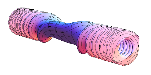
On the other hand, the global boundedness of $\dot{\theta}$ from Assumption 1.(ii) is not necessary for the definition of a non-self-intersecting waveguide. In Figure 4 we present an example of an infinite twisted waveguide with elliptical cross-section such that $\dot{\theta}(s)$ tends to infinity as $|s|\to\infty$. It can be introduced and handled by the methods of Section 3 without problems. However, the form domain of the transformed Laplacian $\tilde{H}_{\varepsilon}$ will not coincide with the Sobolev space $W_{0}^{1,2}(\Omega_{0})$ (i.e. (3.18) will not hold) and an extensive modification of the present strategy to get the operator limit (1.1) would be required.

Figure 4: A waveguide of elliptical cross-section along a straight line whose twisting diverges at infinity. The embedded cylindrical channel is responsible for the existence of essential spectrum.

It is also important to emphasize that the unboundedness of $\dot{\theta}$ may lead to pathological spectral properties. Indeed, the condition $\dot{\theta}(s)\to\infty$ as $|s|\to\infty$ implies that $H_{\mathrm{eff}}$ has purely discrete spectrum, while $\sigma_{\mathrm{ess}}(-\Delta_{D}^{\Omega_{\varepsilon}})\not=\varnothing$ in general. Actually, the latter happens whenever the cross-section $\omega$ contains the origin of $\mathbb{R}^{2}$ (as in Figure 4), so that there is an infinite cylindrical channel in $\Omega_{\varepsilon}$ leading to scattering waves. It does not contradict the validity of the effective Hamiltonian approximation in principle, since the threshold of the essential spectrum of $-\Delta_{D}^{\Omega_{\varepsilon}}-\varepsilon^{-2}E_{1}$ tends to infinity in the limit as $\varepsilon\to 0$, but the usefulness of the approximation becomes doubtful.

We admit that Assumption 2 seems unnatural and it is true that it comes from our technical procedure of mollifying the curvature functions $k_{1},k_{2}$ and $\dot{\theta}$. Although it covers a wide class of waveguides and, in particular, all the previously known results, there are still reasonable situations for which Assumption 2 does not hold, as the following counterexample shows.

Example 6.2.

Let us define the curve $\Gamma^{\mathrm{osc}}:\mathbb{R}\to\mathbb{R}^{3}$ by giving its curvatures:

$$k_{1}^{\mathrm{osc}}(s) :=\begin{cases}\;1,&s\in\Big{(}(n-1+\frac{2k}{2n})\pi,(n-1+\frac{2k+1}{2n})\pi\Big{)},\\ -1,&s\in\Big{(}(n-1+\frac{2k+1}{2n})\pi,(n-1+\frac{2k+2}{2n})\pi\Big{)},\end{cases}\quad n\in\mathbb{N},\;k=0,1...,n-1,$$

$$k_{2}^{\mathrm{osc}}(s) :=0.$$

Figure 5: The counterexample curve.

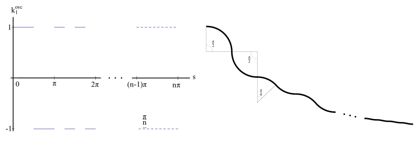
The graph of the function $k_{1}^{\mathrm{osc}}$ is given in Figure 5 as well as $\Gamma^{\mathrm{osc}}$ itself. This curve lies in a plane and consists of arcs of circle of radius $1$ which are shorter and shorter as $s$ grows. For $s\to\infty$, this curve looks like a straight line, however, the curvature is still nonzero. It is possible to show that for all $\varepsilon>0$ there exists $n_{0}\in\mathbb{R}$ such that

$$\sup_{|\eta|\leq\frac{\delta(\varepsilon)}{2}}\int_{(n-1)\pi}^{n\pi}\left|k_{1}^{\mathrm{osc}}(s)-k_{1}^{\mathrm{osc}}(s+\eta)\right|^{2}ds=4\pi\,,\qquad\forall n\in\mathbb{N},\;n\geq n_{0},$$

and this holds true for any choice of function $\delta$. Hence the curvature $k_{1}^{\mathrm{osc}}$ does not satisfy Assumption 2 and our Theorem 2.1 does not apply.

To get at least some information about the dynamics in such a pathological quantum waveguide, we examine the spectrum of the Dirichlet Laplacian $-\Delta_{D}^{\Omega_{\varepsilon}^{\mathrm{osc}}}$ in a untwisted tube with rectangular cross-section constructed along the curve $\Gamma^{\mathrm{osc}}$. It is possible to show that for any positive $\varepsilon$ (such that the tube does not overlap itself)

$$\inf{\sigma_{\mathrm{ess}}\left(-\Delta_{D}^{\Omega_{\varepsilon}^{\mathrm{osc}}}-\frac{E_{1}}{\varepsilon^{2}}\right)}\geq 0\,.$$

On the other hand, assuming that the effective dynamics is governed by (2.3), we have

$$\sigma(H_{\mathrm{eff}})=\sigma_{\mathrm{ess}}(H_{\mathrm{eff}})=\sigma\Big{(}-\Delta_{D}^{\mathbb{R}}-\frac{1}{4}\Big{)}=\Big{[}-\frac{1}{4},\infty\Big{)}.$$

That it, $[-\frac{1}{4},0]$ belongs to the essential spectrum of $H_{\mathrm{eff}}$, while the threshold of the essential spectrum of the three-dimensional renormalized Hamiltonian is non-negative for every positive $\varepsilon$.

Again, this pathological spectral behavior does not necessarily imply that the norm-resolvent convergence of $-\Delta_{D}^{\Omega_{\varepsilon}^{\mathrm{osc}}}-\varepsilon^{-2}E_{1}$ to $H_{\mathrm{eff}}$ does not hold. As a matter of fact, it is possible to show that $-\Delta_{D}^{\Omega_{\varepsilon}^{\mathrm{osc}}}-\varepsilon^{-2}E_{1}$ possesses an infinite number of negative eigenvalues, hence it may happen that these eigenvalues cover the whole interval $[-\frac{1}{4},0]$ in the limit as $\varepsilon\to 0$.

In any case, we would like to emphasize that our Theorem 2.1 represents the first norm-resolvent convergence result for unbounded waveguides in the full setting of bending and twisting . The question of optimality of Assumption 2 in the unbounded case remains open.

6.3 Two-dimensional waveguides

The methods of the present paper also enable one to improve the known results [9, 11] about the effective Hamiltonian approximation in strip-like neighbourhoods of plane curves. The norm-resolvent convergence in the two-dimensional case does not follow directly from our three-dimensional Theorem 2.1, but it can be established exactly in the same way. The proof is in fact much simpler because there is just one curvature function, the Frenet frame always exists (it coincides with a relatively parallel frame) and there is no twisting (codimension of the reference curve is one). Here we therefore present just the ultimate result without proof. The interested reader who is not willing to adapt the present proof to the two-dimensional case himself/herself is referred to [21].

Let $\Gamma:I\to\mathbb{R}^{2}$ be a unit-speed $C^{1}$-smooth curve, where $I$ is an arbitrary open interval (finite, semi-infinite, infinite). The vector fields $T:=\dot{\Gamma}$ and $N:=(-\dot{\Gamma}^{2},\Gamma^{1})$ form a positively oriented Frenet frame of $\Gamma$. We introduce the curvature function $\kappa$ by the Serret-Frenet formula $\dot{T}=-\kappa N$. Note that, contrary to the three-dimensional case, $\kappa$ is allowed to change sign (and the value of the sign depends on the parametrization).

Figure 6: A two-dimensional quantum waveguide.

In analogy with (3.6) and (3.7), the two-dimensional waveguide $\Omega_{\varepsilon}$ is introduced as the image (3.6) where the mapping $\mathcal{L}$ is given now by

$$\mathcal{L}(s,t):=\Gamma(s)+\varepsilon\,t\,N(s)\,,$$

with $(s,t)\in I\times(-1,1)$ (see Figure 6). The unitary transforms (2.1) and (2.4) should be replaced by

$$U_{1} :L^{2}(\Omega_{\varepsilon})\to L^{2}\big{(}\Omega_{0},\varepsilon\;\!h(s,t)\;\!ds\;\!dt\big{)}:\{\psi\mapsto\psi\circ\mathcal{L}^{-1}\}\,,$$

$$U_{2} :L^{2}\big{(}\Omega_{0},\varepsilon^{2}\;\!h(s,t)\;\!ds\;\!dt\big{)}\to L^{2}(\Omega_{0}):\{\psi\mapsto\sqrt{\varepsilon h}\;\!\psi\}\,,$$

where $h(s,t):=1-\varepsilon\kappa(s)t$, and we again define $U:=U_{2}U_{1}$. The latter enables one to approximate in the limit as $\varepsilon\to 0$ the Dirichlet Laplacian in $\Omega_{\varepsilon}$ by the well known one-dimensional effective Hamiltonian

$$H_{\mathrm{eff}}:=-\Delta_{D}^{I}-\frac{\kappa^{2}}{4}\,.$$

The main idea of the proof again consists in replacing $U_{2}$ by (4.4) using the mollification $\kappa^{\varepsilon}$ defined analogously to (2.5).

The two-dimensional version of Theorem 2.1 reads as follows.

Theorem 6.3.

Let the following assumptions hold true:

1. $\Gamma\in W^{2,\infty}_{\mathrm{loc}}(I;\mathbb{R}^{2})$  and  $\kappa\in L^{\infty}(I)$.

2. $\Omega_{\varepsilon}$ does not overlap itself (i.e. $\mathcal{L}$ is injective) for small enough $\varepsilon$.

3. $\displaystyle\lim_{\varepsilon\to 0}\sigma_{\kappa}(\delta(\varepsilon))=0$ for some positive continuous function $\delta$ satisfying (4.1), where $\sigma_{\kappa}$ is defined by (2.6).

Then there exist positive constants $\varepsilon_{0}$ and $C$ such that for all $\varepsilon\leq\varepsilon_{0}$,

$$\left\|U(-\Delta_{D}^{\Omega_{\varepsilon}}-\varepsilon^{-2}E_{1}-i)^{-1}U^{-1}-(H_{\mathrm{eff}}-i)^{-1}\oplus 0^{\bot}\right\|_{\mathcal{B}(L^{2}(\Omega_{0}))}\\ \leq C\,\Big{(}\varepsilon+\varepsilon\;\!\|\dot{\kappa}^{\varepsilon}\|+\sigma_{\kappa}(\delta(\varepsilon))\Big{)}\,,$$

where $0^{\bot}$ denotes the zero operator on the orthogonal complement of the span of $\{\varphi\otimes\mathcal{J}_{1}\,|\,\varphi\in L^{2}(I)\}$ and $U=U_{2}U_{1}$.

6.4 Different boundary conditions

It is well known that the structure of the effective Hamiltonian in the limit (1.1) is a consequence of the choice of Dirichlet boundary conditions on the ‘lateral boundary’ $I\times\partial\omega$. Indeed, there is no geometric potential for Neumann boundary conditions [22] and the limit can have a completely different nature if one considers a combination of Dirichlet and Neuman boundary conditions [18]. On the other hand, our choice of Dirichlet boundary conditions on $(\partial I)\times\omega$ is not essential. In the same manner, we could impose any other type of boundary conditions (Neumann, Robin, periodic, etc), which would lead to an analogue of Theorem 2.1, with the boundary conditions of $H_{\mathrm{eff}}$ changed accordingly. In particular, the choice of periodic boundary conditions enable us to cover the case of tubes about closed (compact) curves.

6.5 Non-thin waveguides

Finally, let us mention that the tricks of the present paper how to deal with quantum waveguides under mild regularity assumptions do not restrict to the effective Hamiltonian approximation. For instance, the usage of the relatively parallel frame instead of the Frenet frame enables one to extend some spectral results for $-\Delta_{D}^{\Omega_{\varepsilon}}$ (with $\varepsilon$ not necessarily small) to the general case of waveguides along merely twice differentiable curves with possibly vanishing curvature. In particular, we have in mind the classical results about the curvature-induced bound states [9, 5] and the recent ones about Hardy-type inequalities due to twisting [10, 17, 19].

Acknowledgement

We are grateful to Denis Borisov for valuable discussions, in particular for his idea how to significantly relax our initial hypotheses about the waveguide regularity. This work has been partially supported by the Czech Ministry of Education, Youth, and Sports within the project LC06002 and by the GACR grant No. P203/11/0701.

References

- [1] N. I. Akhiezer, Theory of approximation, Frederick Ungar Publishing Co., New York, 1956, 2nd augmented Russian edition is available, Moscow, Nauka, 1965.
- [2] R. L. Bishop, There is more than one way to frame a curve, The American Mathematical Monthly 82 (1975), 246–251.
- [3] D. Borisov and G. Cardone, Complete asymptotic expansions for the eigenvalues of the Dirichlet Laplacian in thin three-dimensional rods, ESAIM: Control, Optimisation, and Calculus of Variation, to appear.
- [4] G. Bouchitté, M. L. Mascarenhas, and L. Trabucho, On the curvature and torsion effects in one dimensional waveguides, ESAIM: Control, Optimisation and Calculus of Variations 13 (2007), 793–808.
- [5] B. Chenaud, P. Duclos, P. Freitas, and D. Krejčiřík, Geometrically induced discrete spectrum in curved tubes, Differential Geom. Appl. 23 (2005), no. 2, 95–105.
- [6] C. R. de Oliveira, Quantum singular operator limits of thin Dirichlet tubes via -convergence, Rep. Math. Phys. 66 (2010), 375–406.
- [7] C. R. de Oliveira and A. A. Verri, On the spectrum and weakly effective operator for Dirichlet Laplacian in thin deformed tubes, J. Math. Anal. Appl. 381 (2011), 454–468.
- [8] C. R. de Oliveira and A. A. Verri, On norm resolvent and quadratic form convergences in asymptotic thin spatial waveguides, to appear in Proceedings of Spectral Days 2010, Santiago, Chile, in the book series “Operator Theory: Advances and Application”, Birkhüser, Basel.
- [9] P. Duclos and P. Exner, Curvature-induced bound states in quantum waveguides in two and three dimensions, Rev. Math. Phys. 7 (1995), 73–102.
- [10] T. Ekholm, H. Kovařík, and D. Krejčiřík, A Hardy inequality in twisted waveguides, Arch. Ration. Mech. Anal. 188 (2008), 245–264.
- [11] P. Freitas and D. Krejčiřík, Location of the nodal set for thin curved tubes, Indiana Univ. Math. J. 57 (2008), no. 1, 343–376.
- [12] L. Friedlander and M. Solomyak, On the spectrum of the Dirichlet Laplacian in a narrow infinite strip, Amer. Math. Soc. Transl. 225 (2008), 103–116.
- [13] , On the spectrum of the Dirichlet Laplacian in a narrow strip, Israeli Math. J. 170 (2009), no. 1, 337–354.
- [14] D. Grieser, Thin tubes in mathematical physics, global analysis and spectral geometry, Analysis on Graphs and its Applications, Cambridge, 2007 (P. Exner et al., ed.), Proc. Sympos. Pure Math., vol. 77, Amer. Math. Soc., Providence, RI, 2008, pp. 565–593.
- [15] D. Grieser, Spectra of graph neighborhoods and scattering, Proc. London Math. Soc. 97 (2008), 718-–752.
- [16] T. Kato, Perturbation theory for linear operators, Springer-Verlag, Berlin, 1966.
- [17] D. Krejčiřík, Twisting versus bending in quantum waveguides, Analysis on Graphs and its Applications, Cambridge, 2007 (P. Exner et al., ed.), Proc. Sympos. Pure Math., vol. 77, Amer. Math. Soc., Providence, RI, 2008, pp. 617–636. See arXiv:0712.3371v2 [math–ph] (2009) for a corrected version.
- [18] D. Krejčiřík, Spectrum of the Laplacian in a narrow curved strip with combined Dirichlet and Neumann boundary conditions, ESAIM: Control, Optimisation and Calculus of Variations 15 (2009), 555–568.
- [19] D. Krejčiřík and E. Zuazua, The Hardy inequality and the heat equation in twisted tubes, J. Math. Pures Appl. 94 (2010), 277–303.
- [20] J. Lampart, S. Teufel, and J. Wachsmuth, Effective Hamiltonians for thin Dirichlet tubes with varying cross-section, Mathematical Results in Quantum Physics, Hradec Králové, 2010, xi+274 p., World Scientific, Singapore, 2011, pp. 183–189.
- [21] H. Šediváková, Quantum waveguides under mild regularity assumptions, Diploma Thesis, Czech Technical University, June 2011, Supervisor: D. Krejčiřík. The electronic version is available at http://ssmf.fjfi.cvut.cz/studthes/2008/Sedivakova_thesis.pdf.
- [22] M. Schatzman, On the eigenvalues of the Laplace operator on a thin set with Neumann boundary conditions, Applicable Anal. 61 (1996), 293–306.
- [23] J. Wachsmuth and S. Teufel, Effective Hamiltonians for constrained quantum systems, preprint on arXiv:0907.0351v3 [math-ph] (2009).
- [24] , Constrained quantum systems as an adiabatic problem, Phys. Rev. A 82 (2010), 022112.