Hadronic molecules with both open charm and bottom

Abstract

With the one-boson-exchange model, we study the interaction between the S-wave $D^{(*)}/D^{(*)}_{s}$ meson and S-wave $B^{(*)}/B^{(*)}_{s}$ meson considering the S-D mixing effect. Our calculation indicates that there may exist the $B_{c}$-like molecular states. We estimate their masses and list the possible decay modes of these $B_{c}$-like molecular states, which may be useful to the future experimental search.

I introduction

Carrying out the study of the hadron configuration beyond the conventional $q\bar{q}$ meson and $qqq$ baryon is an intriguing and important research topic. In the past decade, more and more charmonium-like or bottomonium-like states were observed in the $e^{+}e^{-}$ collision Aubert:2005rm ; Aubert:2006ge ; :2007sj , $B$ meson decays Choi:2003ue ; Abe:2004zs ; :2007wga ; Aaltonen:2009tz and even $\gamma\gamma$ fusion processes Uehara:2005qd ; Uehara:2009tx ; Shen:2009vs , which have stimulated the extensive discussion of exotic hadron configurations (for a review see Refs. Swanson:2006st ; Zhu:2007wz ; Nielsen:2009uh ).

In this work, we report on the investigation of hadronic molecules with both open charm and open bottom, where the interaction between the charmed meson ($\mathcal{D}^{(*)}=[D^{(*)0},D^{(*)+},D_{s}^{(*)+}]$) and bottom meson ($\mathcal{B}^{(*)}=[B^{(*)+},B^{(*)0},B_{s}^{(*)0}]$) occurs via the one boson exchange (OBE). These new structures are labeled as the $B_{c}$-like molecules because such systems contain a charm ($c$) quark and an anti-bottom ($\bar{b}$) quark. Because of the special hadron configuration, the prediction of the $B_{c}$-like molecules with masses above 7 GeV can provide important information for further experimental search at facilities such as LHCb and the recently discussed $Z^{0}$ factory Chang:2010am .

This paper is organized as follows. After the introduction, we present the formulas of effective potential of $B_{c}$-like molecules. In Sec. III, the numerical results are given. This work ends with the discussion and conclusion.

II The effective potential of $B_{c}$-like molecules

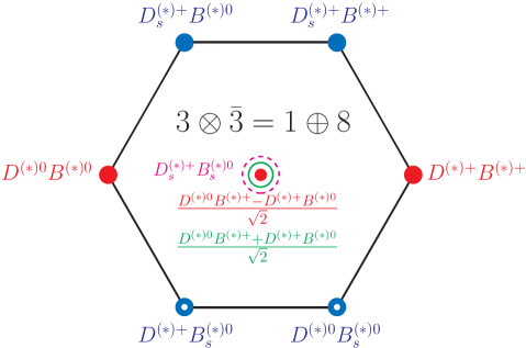
Figure 1: (color online). The flavor wave functions of these hadronic molecular states, which consist of two isosinglets ($a_{s1}=(D^{(*)0}B^{(*)+}+D^{(*)+}B^{(*)0})/\sqrt{2}$, $a_{s2}=D_{s}^{(*)+}B_{s}^{(*)0}$), an isotriplet ($a_{t}=[D^{(*)0}B^{(*)0}$, $(D^{(*)0}B^{(*)+}-D^{(*)+}B^{(*)0})/\sqrt{2}$, $D^{(*)+}B^{(*)+}$]) and two isodoublets ($a_{d1}=[D_{s}^{(*)+}B^{(*)0},D_{s}^{(*)+}B^{(*)+}]$, $a_{d2}=[D^{(*)+}B_{s}^{(*)0},D^{(*)0}B_{s}^{(*)0}]$), where the index $a$ is taken as $X$, $Y$, $Z$ and $\widetilde{Z}$ corresponding to the $\mathcal{DB}$, $\mathcal{D}^{*}\mathcal{B}^{*}$, $\mathcal{D}^{*}\mathcal{B}$ and $\mathcal{D}\mathcal{B}^{*}$ systems, respectively.

The $B_{c}$-like molecules are categorized into four groups, i.e, $\mathcal{DB}$, $\mathcal{D}^{*}\mathcal{B}^{*}$, $\mathcal{D}^{*}\mathcal{B}$ and $\mathcal{D}\mathcal{B}^{*}$. Each group contains nine states, which form an octet and a singlet. Their corresponding flavor wave functions are listed in Fig. 1. We adopt the approach developed in Refs. Tornqvist:1993vu ; Tornqvist:1993ng ; Swanson:2003tb ; Liu:2008fh ; Liu:2008tn ; Thomas:2008ja ; Lee:2009hy ; Sun:2011uh to study the interaction of the $B_{c}$-like molecules. In terms of the Breit approximation, the scattering amplitude $i\mathcal{M}({\mathcal{D}^{(*)}\mathcal{B}^{(*)}}\to{\mathcal{D}^{(*)}\mathcal{B}^{(*)}})$ is related to the interaction potential in the momentum space by the relation

$$\mathcal{V}_{E}(\mathbf{q}) = \frac{-1}{\sqrt{\prod_{i}2M_{i}\prod_{f}2M_{f}}}\mathcal{M}\textnormal{\Huge{$[$}}\raisebox{-13.0pt}{\includegraphics[width=32.52017pt]{am.eps}}\textnormal{\Huge{$]$}},$$

where $M_{i}$ and $M_{j}$ are the masses of the initial and final states, respectively. The potential in the coordinate space $\mathcal{V}(\mathbf{r})$ reads as its Fourier transformation,

$$\mathcal{V}_{E}(\mathbf{r})=\int\frac{d\mathbf{p}}{(2\pi)^{3}}\,e^{i\mathbf{p}\cdot\mathbf{r}}\;\mathcal{V}_{E}(\mathbf{q})\;\mathcal{F}^{2}(q^{2},m_{E}^{2})$$ (1)

where $m_{E}$ is the exchanged meson mass and the monopole form factor (FF) $\mathcal{F}(q^{2},m_{E}^{2})=({\Lambda^{2}-m_{E}^{2}})/({\Lambda^{2}-q^{2}})$ is introduced to depict the structure effect of the vertex of the heavy mesons interacting with the light mesons. The parameter $\Lambda$, which is about one to several GeV, not only denotes the phenomenological cutoff, but also regulates the effective potential.

According to the heavy quark limit and chiral symmetry, the interactions of the light pesudoscalar, vector and scalar mesons with the S-wave heavy flavor mesons were constructed as Cheng:1992xi ; Yan:1992gz ; Wise:1992hn ; Burdman:1992gh ; Casalbuoni:1996pg ; Falk:1992cx

$$\mathcal{L}_{HH\mathbb{P}} = ig\langle H^{(Q)}_{b}\gamma_{\mu}A_{ba}^{\mu}\gamma_{5}\bar{H}^{(Q)}_{a}\rangle$$ (2)

$$+ig\langle\bar{H}^{(\bar{Q})}_{a}\gamma_{\mu}A_{ab}^{\mu}\gamma_{5}H_{b}^{(\bar{Q})}\rangle,$$

$$\mathcal{L}_{HH\mathbb{V}} = i\beta\langle H^{(Q)}_{b}v_{\mu}(\mathcal{V}^{\mu}_{ba}-\rho^{\mu}_{ba})\bar{H}^{(Q)}_{a}\rangle$$ (3)

$$+i\lambda\langle H^{(Q)}_{b}\sigma_{\mu\nu}F^{\mu\nu}(\rho)\bar{H}^{(Q)}_{a}\rangle$$

$$-i\beta\langle\bar{H}^{(\bar{Q})}_{a}v_{\mu}(\mathcal{V}^{\mu}_{ab}-\rho^{\mu}_{ab})H^{(\bar{Q})}_{b}\rangle$$

$$+i\lambda\langle H_{b}^{(\bar{Q})}\sigma_{\mu\nu}F^{\prime\mu\nu}(\rho)\bar{H}^{(\bar{Q})}_{a}\rangle,$$

$$\mathcal{L}_{HH\sigma} = g_{s}\langle H^{(Q)}_{a}\sigma\bar{H}^{(Q)}_{a}\rangle+g_{s}\langle\bar{H}^{(\bar{Q})}_{a}\sigma H^{(\bar{Q})}_{a}\rangle,$$ (4)

where the multiplet fields are expressed as $H_{a}^{(Q)}=\frac{1+\hbox to0.0pt{/\hss}v}{2}[{\mathcal{P}}^{*}_{a\mu}\gamma^{\mu}-{\mathcal{P}}_{a}\gamma_{5}]$, $H^{(\bar{Q})}=[\widetilde{P}_{a}^{*\mu}\gamma_{\mu}-\widetilde{P}_{a}\gamma_{5}]\ \frac{1-\hbox to0.0pt{/\hss}v}{2}$, $\bar{H}=\gamma_{0}H^{\dagger}\gamma_{0}$ with $v=(1,{\mathbf{0}})$, ${\mathcal{P}}^{(*)T}=(D^{(*)0},D^{(*)+},D_{s}^{(*)+})$ or $(B^{(*)-},\bar{B}^{(*)0},\bar{B}_{s}^{(*)0})$, $\widetilde{{\mathcal{P}}}^{(*)T}=(\bar{D}^{(*)0},D^{(*)-},D_{s}^{(*)-})$ or $(B^{(*)+},{B}^{(*)0},{B}_{s}^{(*)0})$, which satisfy the normalization relations $\langle 0|{\mathcal{P}}|Q\bar{q}(0^{-})\rangle=\langle 0|\widetilde{\mathcal{P}}|\bar{Q}q(0^{-})\rangle=\sqrt{M_{\mathcal{P}}}$ and $\langle 0|{\mathcal{P}}^{*}_{\mu}|Q\bar{q}(1^{-})\rangle=\langle 0|\widetilde{\mathcal{P}}^{*}_{\mu}|\bar{Q}q(1^{-})\rangle=\epsilon_{\mu}\sqrt{M_{\mathcal{P}^{*}}}$. The axial current reads as $A^{\mu}=\frac{1}{2}(\xi^{\dagger}\partial_{\mu}\xi-\xi\partial_{\mu}\xi^{\dagger})=\frac{i}{f_{\pi}}\partial_{\mu}{\mathbb{P}}+\cdots$ with $\xi=\exp(i\mathbb{P}/f_{\pi})$ and $f_{\pi}=132$ MeV. $\rho^{\mu}_{ba}=ig_{V}\mathbb{V}^{\mu}_{ba}/\sqrt{2}$, $F_{\mu\nu}(\rho)=\partial_{\mu}\rho_{\nu}-\partial_{\nu}\rho_{\mu}+[\rho_{\mu},{\ }\rho_{\nu}]$, $F^{\prime}_{\mu\nu}(\rho)=\partial_{\mu}\rho_{\nu}-\partial_{\nu}\rho_{\mu}-[\rho_{\mu},{\ }\rho_{\nu}]$ and $g_{V}=m_{\rho}/f_{\pi}$, with $g_{V}=5.8$. In the above expressions, $\mathbb{P}$ and $\mathbb{V}$ denote the three by three pseudoscalar and vector matrices, respectively, i.e.,

$$\mathbb{P} = \left(\begin{array}[]{ccc}\frac{\pi^{0}}{\sqrt{2}}+\frac{\eta}{\sqrt{6}}&\pi^{+}&K^{+}\\ \pi^{-}&-\frac{\pi^{0}}{\sqrt{2}}+\frac{\eta}{\sqrt{6}}&K^{0}\\ K^{-}&\bar{K}^{0}&-\frac{2\eta}{\sqrt{6}}\end{array}\right),$$ (8)

$$\mathbb{V} = \left(\begin{array}[]{ccc}\frac{\rho^{0}}{\sqrt{2}}+\frac{\omega}{\sqrt{2}}&\rho^{+}&K^{*+}\\ \rho^{-}&-\frac{\rho^{0}}{\sqrt{2}}+\frac{\omega}{\sqrt{2}}&K^{*0}\\ K^{*-}&\bar{K}^{*0}&\phi\end{array}\right).$$ (12)

The coupling constants involved in Eqs. (2)-(4) include $g=0.59$ extracted from the experimental width of $D^{*+}$  Isola:2003fh , $\beta=0.9$ determined by the vector meson dominance mechanism, $\lambda=0.56$ GeV^-1 obtained by comparing the form factor calculated by light cone sum rule with the one obtained by lattice QCD. In addition, the coupling constant related to the scalar meson $\sigma$, $g_{s}=g_{\pi}/(2\sqrt{6})$ with $g_{\pi}=3.73$ was given in Ref. Falk:1992cx . In the heavy quark limit, the interactions of the $\mathcal{D}^{(*)}\mathcal{D}^{(*)}$ and $\mathcal{B}^{(*)}\mathcal{B}^{(*)}$ with light mesons are the same.

With these Lagrangians listed in Eq. (2)-(4), we can deduce the expressions of $\mathcal{V}_{E}(\mathbf{r})$. When obtaining the total effective potentials, we sandwich $\mathcal{V}_{E}(\mathbf{r})$ between the corresponding $B_{c}$-like molecular states. Thus, the general expression of the total effective potential is expressed as

$$\mathcal{V}_{Total}^{\,\,a_{\xi}}(\mathbf{r})=\Big{\langle}a_{\xi}[J]\Big{|}\sum_{E=\pi,\eta,\rho,\omega,...}\mathcal{V}_{E}(\mathbf{r})\Big{|}a_{\xi}[J]\Big{\rangle},$$ (13)

where subscript $a_{\xi}$ with $\xi=s1,s2,t,d1,d2$ and $a=X,Y,Z,\widetilde{Z}$ is introduced to distinguish the total effective potentials of the molecular systems defined in Fig. 1. $J$ denotes the total angular momentum of system ($J=0$, $J=1$, $J=0,1,2$ for the $\mathcal{DB}$, $\mathcal{D^{*}B}/\mathcal{DB}^{*}$ and $\mathcal{D^{*}B}^{*}$ systems respectively). The definitions of $\left|a_{\xi}[J]\right\rangle$ are

$$\left|X_{\xi}[0]\right\rangle = \left|\mathcal{DB}(^{1}S_{0})\right\rangle,$$

$$\left|Z_{\xi}[1]\right\rangle = \left(\left|\mathcal{D^{*}B}(^{3}S_{1})\right\rangle,\left|\mathcal{D^{*}B}(^{3}D_{1})\right\rangle\right)^{T},$$

$$\left|\widetilde{Z}_{\xi}[1]\right\rangle = \left(\left|\mathcal{DB^{*}}(^{3}S_{1})\right\rangle,\left|\mathcal{DB^{*}}(^{3}D_{1})\right\rangle\right)^{T},$$

$$\left|Y_{\xi}[0]\right\rangle = \left(\left|\mathcal{D^{*}B^{*}}(^{3}S_{0})\right\rangle,\left|\mathcal{D^{*}B^{*}}(^{5}D_{0})\right\rangle\right)^{T},$$

$$\left|Y_{\xi}[1]\right\rangle = \left(\left|\mathcal{D^{*}B^{*}}(^{3}S_{1})\right\rangle,\left|\mathcal{D^{*}B^{*}}(^{3}D_{1})\right\rangle,\left|\mathcal{D^{*}B^{*}}(^{5}D_{1})\right\rangle\right)^{T},$$

$$\left|Y_{\xi}[2]\right\rangle = \big{(}\left|\mathcal{D^{*}B^{*}}(^{5}S_{2})\right\rangle,\left|\mathcal{D^{*}B^{*}}(^{1}D_{2})\right\rangle,\left|\mathcal{D^{*}B^{*}}(^{3}D_{2})\right\rangle,$$

$$\left|\mathcal{D^{*}B^{*}}(^{5}D_{2})\right\rangle\big{)}^{T},$$

with

$$\Big{|}\mathcal{DB}^{*}/\mathcal{D}^{*}\mathcal{B}\big{(}^{2S+1}L_{J}\big{)}\Big{\rangle}=\sum_{m,m_{L},m_{S}}C_{1m,Lm_{L}}^{JM}|\epsilon^{m}_{n};L,m_{L}\rangle,$$ (14)

$$\Big{|}\mathcal{D}^{*}\mathcal{B}^{*}\big{(}^{2S+1}L_{J}\big{)}\Big{\rangle}=\sum_{m,m^{\prime},m_{L},m_{S}}C_{Sm_{S},Lm_{L}}^{JM}C_{1m,1m^{\prime}}^{Sm_{S}}|\epsilon^{m^{\prime}}_{n^{\prime}}\epsilon^{m}_{n};L,m_{L}\rangle,$$

where $C_{1m,Lm_{L}}^{JM}$, $C_{Sm_{S},Lm_{L}}^{JM}$ and $C_{1m,1m^{\prime}}^{Sm_{S}}$ denote the Clebsch-Gordan coefficients. The polarization vector for the vector heavy flavor meson is written as $\epsilon^{m}_{\pm}=\mp\frac{1}{\sqrt{2}}(\epsilon^{m}_{x}\pm i\epsilon^{m}_{y})$ and $\epsilon^{m}_{0}=\epsilon^{m}_{z}$. In the above expressions, ${}^{2S+1}L_{J}$ is applied to denote the total spin $S$, angular momentum $L$, total angular momentum $J$ of the $\mathcal{D}^{(*)}\mathcal{B}^{(*)}$ systems, while $L=S$ and $L=D$ are introduced to distinguish S-wave and D-wave interactions. Because of the S-D mixing effect, the obtained total effective potentials of the $\mathcal{D^{*}B}$, $\mathcal{DB^{*}}$ and $\mathcal{D^{*}B^{*}}$ molecular systems are in matrix form. The total effective potentials are composed of subpotentials as shown in Table. 1.

Table 1: The relation of the total effective potential $\mathcal{V}_{Total}^{\,\,a_{\xi}}(r)$ and the subpotentials. Here, $\varpi$ is taken as 3 and -1 corresponding to the states marked by the subscripts $s1$ and $t$, respectively. Since the total effective potential of the $\mathcal{DB}^{*}$ systems is the same as that of the $\mathcal{D^{*}B}$ systems, we only show the result for $\mathcal{D^{*}B}$. We use $-$ to denote the case when the OBE potential does not exist since no suitable meson exchange is allowed for these systems.

$a_{\xi}$	$X_{s1}/X_{t}$	$X_{s2}$	$X_{d1}/X_{d2}$
$\mathcal{V}_{Total}^{\,\,a_{\xi}}(r)$	$V_{\sigma}^{\mathcal{DB}}+\frac{\varpi}{2}V_{\rho}^{\mathcal{DB}}+\frac{1}{2}V_{\omega}^{\mathcal{DB}}$	$V_{\phi}^{\mathcal{DB}}$	$-$
$a_{\xi}$	$Y_{s1}/Y_{t}$	$Y_{s2}$	$Y_{d1}/Y_{d2}$
$\mathcal{V}_{Total}^{\,\,a_{\xi}}(r)$	$V_{\sigma}^{\mathcal{D^{*}B^{*}}}+\frac{\varpi}{2}V_{\rho}^{\mathcal{D^{*}B^{*}}}+\frac{1}{2}V_{\omega}^{\mathcal{D^{*}B^{*}}}$	$V_{\phi}^{\mathcal{D^{*}B^{*}}}+\frac{2}{3}V_{\eta}^{\mathcal{D^{*}B^{*}}}$	$-\frac{2}{3}V_{\eta}^{\mathcal{D^{*}B^{*}}}$
	$+\frac{\varpi}{2}V_{\pi}^{\mathcal{D^{*}B^{*}}}+\frac{1}{6}V_{\eta}^{\mathcal{D^{*}B^{*}}}$
$a_{\xi}$	$Z_{s1}/Z_{t}$	$Z_{s2}$	$Z_{d1}/Z_{d2}$
$\mathcal{V}_{Total}^{\,\,a_{\xi}}(r)$	$V_{\sigma}^{\mathcal{D^{*}B}}+\frac{\varpi}{2}V_{\rho}^{\mathcal{D^{*}B}}+\frac{1}{2}V_{\omega}^{\mathcal{D^{*}B}}$	$V_{\phi}^{\mathcal{D^{*}B}}$	$-$

The expressions of the subpotentials are

$$V^{\mathcal{DB}}_{\sigma} = -g_{s}^{2}Y(\Lambda,m_{\sigma},r),\quad V^{\mathcal{DB}}_{{}_{\mathbb{V}}}=-\frac{1}{2}\beta^{2}g_{V}^{2}Y(\Lambda,m_{{}_{\mathbb{V}}},r),$$

$$V^{\mathcal{D^{*}B}}_{\sigma} = -g_{s}^{2}Y(\Lambda,m_{\sigma},r)\,\mathrm{diag}(1,1),$$

$$V^{\mathcal{D^{*}B}}_{{}_{\mathbb{V}}} = -\frac{1}{2}\beta^{2}g_{V}^{2}Y(\Lambda,m_{{}_{\mathbb{V}}},r)\,\mathrm{diag}(1,1),$$

$$V^{\mathcal{D^{*}B^{*}}}_{\sigma} = -g_{s}^{2}\mathcal{A}[J]Y(\Lambda,m_{\sigma},r),$$

$$V^{\mathcal{D^{*}B^{*}}}_{{}_{\mathbb{V}}} = -\frac{1}{4}\bigg{\{}2\beta^{2}g_{V}^{2}\mathcal{A}[J]-8\lambda^{2}g_{V}^{2}\bigg{(}\frac{2}{3}\mathcal{B}[J]\nabla^{2}$$

$$-\frac{1}{3}\mathcal{C}[J]r\frac{\partial}{\partial r}\frac{1}{r}\frac{\partial}{\partial r}\bigg{)}\bigg{\}}Y(\Lambda,m_{{}_{\mathbb{V}}},r),$$

$$V^{\mathcal{D^{*}B^{*}}}_{{}_{\mathbb{P}}} = -\frac{g^{2}}{f_{\pi}^{2}}\bigg{[}\frac{1}{3}\mathcal{B}[J]\nabla^{2}+\frac{1}{3}\mathcal{C}[J]r\frac{\partial}{\partial r}\frac{1}{r}\frac{\partial}{\partial r}\bigg{]}Y(\Lambda,m_{{}_{\mathbb{P}}},r)$$

with $Y(\Lambda,m_{E},r)=\frac{1}{4\pi r}(e^{-m_{E}\,r}-e^{-\Lambda r})-\frac{\Lambda^{2}-m_{E}^{2}}{8\pi\Lambda}e^{-\Lambda r},$ where we use superscripts $\mathcal{D}^{(*)}\mathcal{B}^{(*)}$ to distinguish these subpotentials for the different systems while the introduced subscripts $\mathbb{P}$ and $\mathbb{V}$ denote the corresponding light pseudoscalar and vector meson exchanges respectively. $m_{E}$ denotes the mass of exchange meson. Matrices $\mathcal{A}[J]$, $\mathcal{B}[J]$ and $\mathcal{C}[J]$ are listed below with $\mathcal{A}[0]=\mathrm{diag}(1,1)$, $\mathcal{A}[1]=\mathrm{diag}(1,1,1)$, $\mathcal{A}[2]=\mathrm{diag}(1,1,1,1)$, $\mathcal{B}[0]=\mathrm{diag}(2,-1)$, $\mathcal{B}[1]=\mathrm{diag}(1,1,-1)$, $\mathcal{B}[2]=\mathrm{diag}(-1,1,1,-1)$, $\mathcal{C}[0]=\left(\begin{array}[]{cc}0&\sqrt{2}\\ \sqrt{2}&2\\ \end{array}\right)$, $\mathcal{C}[1]=\left(\begin{array}[]{ccc}0&-\sqrt{2}&0\\ -\sqrt{2}&1&0\\ 0&0&1\\ \end{array}\right)$ and $\mathcal{C}[2]=\left(\begin{array}[]{cccc}0&\sqrt{\frac{2}{5}}&0&-\sqrt{\frac{14}{5}}\\ \sqrt{\frac{2}{5}}&0&0&-\frac{2}{\sqrt{7}}\\ 0&0&-1&0\\ -\sqrt{\frac{14}{5}}&-\frac{2}{\sqrt{7}}&0&-\frac{3}{7}\\ \end{array}\right)$. In addition, the kinetic terms for the $\mathcal{B^{(*)}D^{(*)}}$ systems are

$$K_{\mathcal{DB}} = -\frac{\triangle}{2\tilde{m}_{1}},$$

$$K_{\mathcal{D^{*}B}/\mathcal{DB^{*}}} = \mathrm{diag}\Bigg{(}-\frac{\triangle}{2\tilde{m}_{2}},~{}-\frac{\triangle_{2}}{2\tilde{m}_{2}}\Bigg{)},$$

$$K_{\mathcal{B^{*}D^{*}}[J=0]} = \mathrm{diag}\Bigg{(}-\frac{\triangle}{2\tilde{m}_{3}},~{}-\frac{\triangle_{2}}{2\tilde{m}_{3}}\Bigg{)},$$

$$K_{\mathcal{B^{*}D^{*}}[J=1]} = \mathrm{diag}\Bigg{(}-\frac{\triangle}{2\tilde{m}_{3}},~{}-\frac{\triangle_{2}}{2\tilde{m}_{3}},~{}-\frac{\triangle_{2}}{2\tilde{m}_{3}}\Bigg{)},$$

$$K_{\mathcal{B^{*}D^{*}}[J=2]} = \mathrm{diag}\Bigg{(}-\frac{\triangle}{2\tilde{m}_{3}},~{}-\frac{\triangle_{2}}{2\tilde{m}_{3}},~{}-\frac{\triangle_{2}}{2\tilde{m}_{3}},~{}-\frac{\triangle_{2}}{2\tilde{m}_{3}}\Bigg{)},$$

where $\triangle=\frac{1}{r^{2}}\frac{\partial}{\partial r}r^{2}~{}\frac{\partial}{\partial r}$, $\triangle_{2}=\triangle-{6\over{r^{2}}}$. $\tilde{m}_{1}$, $\tilde{m}_{2}$ and $\tilde{m}_{3}$ are the reduced masses of the corresponding systems.

III numerical result

With the above preparation, in the following we illustrate the numerical results for the $B_{c}$-like molecular systems. In order to obtain the information of the bound-state solutions (binding energy and root-mean-square radius) of systems listed in Fig. 1, we need to solve the coupled channel Schrödinger equation with the deduced effective potentials, which can answer whether these $B_{c}$-like molecular states exist or not. Here, we adopt FESSDE, a Fortran program for solving the coupled channel Schrödinger equation Abrashkevich1995 ; Abrashkevich1998 , to numerically obtain the binding energy and the corresponding root-mean-square radius. Additionally we also use a MATLAB package MATSCE matscs to do a cross-check. Usually the OBE potential is suitable to describe the interaction of a loosely bound state. Thus, we require the obtained binding energy in the range of $0\sim-20$ MeV and the cutoff in the range of $1\sim 5$ GeV when presenting the result.

Table 2: The typical values of the obtained bound-state solutions for the $\mathcal{D^{(*)}B^{(*)}}$ systems. Here, $\Lambda$, $E$, and $r_{\mathrm{RMS}}$ are in units of GeV, MeV, and fm, respectively.

System	State	$\Lambda/E/r_{\mathrm{RMS}}$	State	$\Lambda/E/r_{\mathrm{RMS}}$	System	State	$\Lambda/E/r_{\mathrm{RMS}}$
$\mathcal{DB}$	$X_{s1}$	1.3/-1.28/2.58	$X_{s2}$	3.2/-2.03/1.99	$\mathcal{D^{*}B}$	$Z_{s1}$	1.3/-2.10/2.07
		1.4/-6.14/1.35		4.0/-10.87/0.94			1.4/-7.92/1.19
		1.5/-13.91/0.98		4.8/-21.90/0.69			1.5/-16.69/0.89
$\mathcal{DB^{*}}$	$\tilde{Z}_{s1}$	1.3/-1.32/2.60	$\tilde{Z}_{s2}$	3.0/-0.76/3.12		$Z_{s2}$	3.0/-1.83/2.04
		1.4/-6.21/1.34		3.5/-4.96/1.32			3.5/-7.55/1.08
		1.5/-14.02/0.97		4.0/-11.06/0.93			4.0/-15.08/0.80

System	State	$\Lambda/E/r_{\mathrm{RMS}}$	State	$\Lambda/E/r_{\mathrm{RMS}}$	State	$\Lambda/E/r_{\mathrm{RMS}}$	State	$\Lambda/E/r_{\mathrm{RMS}}$	State	$\Lambda/E/r_{\mathrm{RMS}}$
$\mathcal{D^{*}B^{*}}$	$Y_{s1}^{J=0}$	1.25/-2.70/2.00	$Y_{s2}^{J=0}$	1.9/-1.66/2.12	$Y_{t}^{J=0}$	2.5/-2.23/1.82	$Y_{d1}^{J=0}$	3.3/-0.94/2.61	$Y_{d2}^{J=0}$	3.4/-1.62/2.03
		1.30/-8.82/1.25		1.95/-6.65/1.13		2.7/-8.04/1.01		3.4/-5.10/1.14		3.5/-6.53/1.03
		1.35/-19.47/0.94		2.00/-17.77/0.74		2.9/-18.64/0.69		3.5/-12.41/0.75		3.6/-14.64/0.70
	$Y_{s1}^{J=1}$	1.25/-3.59/1.76	$Y_{s2}^{J=1}$	1.96/-1.05/2.64	$Y_{t}^{J=1}$	4.27/-3.20/1.53	$Y_{d1}^{J=1}$	4.98/-1.08/2.46
		1.30/-8.98/1.22		2.05/-6.92/1.13		4.54/-10.85/0.87		4.99/-1.27/2.26
		1.35/-17.40/0.95		2.14/-18.81/0.74		4.81/-24.74/0.60		5.00/-1.49/2.10
	$Y_{s1}^{J=2}$	0.96/-1.28/2.59	$Y_{s2}^{J=2}$	2.0/-2.50/1.80
		1.05/-7.99/1.25		2.1/-7.25/1.14
		1.14/-20.12/0.90		2.2/-14.63/0.87

In Table 2, we list the obtained typical values of the bound-state solution of these $B_{c}$-like molecular systems, while the dependence of the results on $\Lambda$ is given in Fig. 2. Among the 24 cases shown in Table. 1, we find that there exist the bound-state solutions only for 17 states:

1. $\mathcal{DB}$: We find the bound-state solution only for the $X_{s1}$ and $X_{s2}$ states. Both of these states are of the same quantum number, i.e., $I(J^{P})=0(0^{+})$. The values of the cutoff $\Lambda$ is close to 1 GeV for the $X_{s1}$ state. For the other isosinglet $X_{s2}$, the bound-state solution appears when taking $\Lambda\sim 3.2$ GeV.

2. $\mathcal{D^{*}B}/\mathcal{DB^{*}}$: The bound-state solution exists only for the four isosinglets $Z_{s1}$, $Z_{s2}$, $\tilde{Z}_{s1}$ and $\tilde{Z}_{s2}$ with $0(1^{+})$. Since the effective potentials of the $\mathcal{D^{*}B}$ and $\mathcal{DB^{*}}$ systems are the same, the dependence of the bound solutions on $\Lambda$ for $Z_{s1}$ and $Z_{s2}$ are almost similar to those of $\tilde{Z}_{s1}$ and $\tilde{Z}_{s1}$ respectively (see Fig. 2). The small difference of the reduced masses also results in the difference of the typical values listed in Table. 2 when comparing the results of the states marked by the same subscript $s1$ or $s2$.

3. $\mathcal{D^{*}B^{*}}$: For the $\mathcal{D^{*}B^{*}}$ systems, there are 15 states. Among them we find 11 states with bound-state solutions, which include the isosinglets $Y_{s1}^{J=0}$, $Y_{s2}^{J=0}$, $Y_{s1}^{J=1}$, $Y_{s2}^{J=1}$, $Y_{s1}^{J=2}$, $Y_{s2}^{J=2}$, isodoublets $Y_{d1}^{J=0}$, $Y_{d2}^{J=0}$, $Y_{d1}^{J=1}$, and isodoublets $Y_{t}^{J=0}$, $Y_{t}^{J=1}$.

We use a hand-waving notation, i.e., five-star, four-star, three-star and two-star etc to mark the states in order to indicate that the bound-state solutions exist when the cutoff parameter $\Lambda$ corresponds to the different values: $\Lambda<1.5$ GeV, $1.5<\Lambda<2.5$ GeV, $2.5<\Lambda<3.5$ GeV, $3.5<\Lambda<5$ GeV respectively. In this way we categorize these states according to the numerical results listed in Fig. 2 and Table 2 (see Table 3 for more details). Usually the cutoff $\Lambda$ is taken around 1 GeV, which is a reasonable value, especially in the deuteron case. Thus, a five-star state implies that a loosely molecular state probably exists. The mass spectra of the $B\bar{D}$, $B\bar{D}^{*}$, $B^{*}\bar{D}$, and $B^{*}\bar{D}^{*}$ molecular states with the $\{Q\bar{q}\}\{\bar{Q}^{(\prime)}q\}$ configuration were studied with the QCD sum rule approach Zhang:2009vs , which correspond to the above six five-star $B_{c}$-like molecular states obtained in this work.

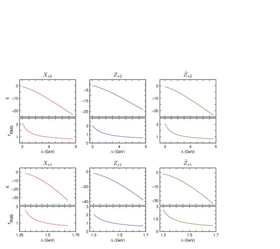
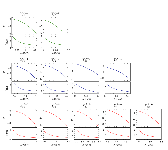
Figure 2: (color online). The variation of the binding energy $E$ and root-mean-square radius $r_{RMS}$ with $\Lambda$ for the $\mathcal{D}^{(*)}\mathcal{B}^{(*)}$ system. Here $E$ and $r_{RMS}$ are in units of MeV and fm. The superscript $J=0$, $J=1$, $J=2$ denotes the total angular momentum $J$.

Table 3: Summary of the $B_{c}$-like systems.

	State	$I(J^{P})$	Remark		State	$I(J^{P})$	Remark	State	$I(J^{P})$	Remark
$\mathcal{DB}$	$X_{s1}$	$0(0^{+})$	$\star\star\star\star\star$		$Y^{J=0}_{s1}$	$0(0^{+})$	$\star\star\star\star\star$	$Y^{J=1}_{s2}$	$0(1^{+})$	$\star\star\star\star$
	$X_{s2}$	$0(0^{+})$	$\star\star\star$		$Y^{J=0}_{s2}$	$0(0^{+})$	$\star\star\star\star$	$Y^{J=1}_{s1}$	$1(1^{+})$	$\star\star$
$\mathcal{D^{*}B}$	$Z_{s1}$	$0(1^{+})$	$\star\star\star\star\star$	$\mathcal{D^{*}B^{*}}$	$Y^{J=0}_{t}$	$1(0^{+})$	$\star\star\star\star$	$Y^{J=1}_{d1}$	$\frac{1}{2}(1^{+})$	$\star\star$
	$Z_{s2}$	$0(1^{+})$	$\star\star\star$		$Y^{J=0}_{d1}$	$\frac{1}{2}(0^{+})$	$\star\star\star$	$Y^{J=2}_{s1}$	$0(2^{+})$	$\star\star\star\star\star$
$\mathcal{DB^{*}}$	$\tilde{Z}_{s1}$	$0(1^{+})$	$\star\star\star\star\star$		$Y^{J=0}_{d2}$	$\frac{1}{2}(0^{+})$	$\star\star\star$	$Y^{J=2}_{s2}$	$0(2^{+})$	$\star\star\star\star$
	$\tilde{Z}_{s2}$	$0(1^{+})$	$\star\star\star$		$Y^{J=1}_{s1}$	$0(1^{+})$	$\star\star\star\star\star$

In the following, we will discuss the allowed decay modes of these predicted $B_{c}$-like molecular states that may be helpful to the future experimental search. All the five-star states $X_{s1}$, $Z_{s1}$, $\tilde{Z}_{s1}$, $Y_{s1}^{J=0}$, $Y_{s1}^{J=1}$ and $Y_{s1}^{J=2}$ are the isosinglet with subscript $s1$. Their decay modes are listed in the 2nd-7th columns of Table. 4, respectively. In addition, the decays of the four four-star states $Y_{s2}^{J=0}$, $Y_{t}^{J=0}$, $Y_{s2}^{J=1}$ and $Y_{s2}^{J=2}$ are shown in the 8th-11th columns of Table. 4, respectively. In Table. 4, we also give the decay modes of the remaining five three-star states. In these decay channels, the $B_{c}(1P_{1})$ and $B_{c}^{\prime}(1P_{1})$ mesons are the mixture of the $1^{1}P_{1}$ and $1^{3}P_{1}$ states Ebert:2011jc : $|B_{c}(1P_{1})\rangle=|B_{c}(1^{1}P_{1})\rangle\cos\theta+|B_{c}(1^{3}P_{1})\rangle\sin\theta$, $|B_{c}^{\prime}(1P_{1})\rangle=-|B_{c}(1^{1}P_{1})\rangle\sin\theta+|B_{c}(1^{3}P_{1})\rangle\cos\theta$. At present only $B_{c}(1^{1}S_{0})$ was observed with a mass $m(B_{c}(1^{1}S_{0}))=6277$ MeV Nakamura:2010zzi . We adopt the theoretical values from Ref. Ebert:2011jc when giving the decay channels of these $B_{c}$-like molecular states, i.e., $M_{B_{c}(1^{3}S_{1})}=6333$ MeV, $M_{B_{c}(2^{1}S_{0})}=6842$ MeV, $M_{B_{c}(2^{3}S_{1})}=6882$ MeV, $M_{B_{c}(1^{3}P_{0})}=6699$ MeV, $M_{B_{c}(1P_{1})}=6743$ MeV, $M_{B_{c}^{\prime}(1P_{1})}=6750$ MeV and $M_{B_{c}(1^{3}P_{2})}=6761$ MeV Ebert:2011jc . In obtaining these decay channels, we have only considered the ground state of the light meson.

Table 4: The decay modes of the predicted $B_{c}$ like molecular states. Here, $\checkmark$ denotes that the corresponding decay mode is allowed.

channels

$X_{s1}$

$Z_{s1}$

$\widetilde{Z}_{s1}$

$Y^{J=0}_{s1}$

$Y^{J=1}_{s1}$

$Y^{J=2}_{s1}$

$Y_{s2}^{J=2}$

$Y_{t}^{J=0}$

$Y_{s2}^{J=1}$

$Y_{s2}^{J=2}$

$X_{s2}$

$Z_{s2}$

$\widetilde{Z}_{s2}$

$Y^{J=0}_{d1}$

$Y^{J=0}_{d2}$

$BD$

✓

✓

✓

$BD^{*}$

✓

✓

$B^{*}D$

✓

✓

✓

$BD_{s}$

✓

✓

$B_{s}D$

✓

✓

$B_{s}^{*}D^{*}$

✓

$B_{s}D_{s}$

✓

✓

$B_{s}D_{s}^{*}$

✓

✓

$B_{s}^{*}D_{s}$

✓

✓

✓

$B_{c}(1^{1}S_{0})\omega$

✓

✓

✓

✓

✓

$B_{c}(1^{3}S_{1})\omega$

✓

✓

✓

✓

✓

✓

$B_{c}(1^{1}S_{0})\eta^{(\prime)}$

✓

✓

✓

✓

✓

$B_{c}(1^{3}S_{1})\eta$

✓

✓

✓

✓

✓

✓

✓

✓

$B_{c}(1^{3}S_{1})\eta^{\prime}$

✓

✓

✓

✓

✓

✓

$B_{c}(1^{3}P_{0})\eta$

✓

✓

✓

✓

✓

$B_{c}(1P_{1})\eta$

✓

✓

✓

✓

✓

✓

✓

✓

✓

$B_{c}^{\prime}(1P_{1})\eta$

✓

✓

✓

✓

✓

✓

✓

✓

✓

$B_{c}(1^{3}P_{2})\eta$

✓

✓

✓

✓

✓

✓

$B_{c}(2^{1}S_{0})\eta$

✓

✓

$B_{c}(2^{3}S_{1})\eta$

✓

✓

✓

$B_{c}(1^{1}S_{0})\pi$

✓

$B_{c}(2^{1}S_{0})\pi$

✓

$B_{c}(1P_{1})\pi$

✓

$B_{c}^{\prime}(1P_{1})\pi$

✓

$B_{c}(1^{3}S_{1})\rho$

✓

$B_{c}(1^{1}S_{0})\phi$

✓

✓

✓

✓

$B_{c}(1^{3}S_{1})\phi$

✓

✓

✓

✓

✓

$B_{c}(1^{1}S_{0})\pi\pi$

✓

✓

✓

$B_{c}(1^{3}S_{1})\pi\pi$

✓

✓

✓

✓

✓

✓

$B_{c}(1^{3}P_{0})\pi\pi$

✓

✓

✓

$B_{c}(1P_{1})\pi\pi$

✓

✓

✓

✓

$B_{c}^{\prime}(1P_{1})\pi\pi$

✓

✓

✓

✓

$B_{c}(1^{3}P_{2})\pi\pi$

✓

✓

✓

✓

✓

✓

$B_{c}(2^{1}S_{0})\pi\pi$

✓

✓

✓

$B_{c}(2^{3}S_{1})\pi\pi$

✓

✓

✓

✓

✓

$B_{c}(1^{1}S_{0})K\bar{K}$

✓

✓

$B_{c}(1^{3}S_{1})K\bar{K}$

✓

✓

✓

IV Discussion and conclusion

In short summary, we have studied the interaction between the S-wave $D^{(*)}/D^{(*)}_{s}$ meson and S-wave $B^{(*)}/B^{(*)}_{s}$ meson in the OBE model. With the obtained effective potentials, we predict the existence of many $B_{c}$-like molecular states where we have already included the S-D mixing effect. Besides estimating their mass spectrum, we also list their decay modes.

Table 5: The bound-state solutions of $Y_{s1}^{J=0}$, $Y_{s1}^{J=1}$ and $Y_{s1}^{J=2}$ only considering OPE potentials. Here, $E$, $\Lambda$, and $r_{\mathrm{RMS}}$ are in units of GeV, GeV, and fm, respectively.

State	$\Lambda/E/r_{\mathrm{RMS}}$	State	$\Lambda/E/r_{\mathrm{RMS}}$	State	$\Lambda/E/r_{\mathrm{RMS}}$
$Y_{s1}^{J=0}$	2.1/-2.45/2.06	$Y_{s1}^{J=1}$	2.4/-1.73/2.34	$Y_{s1}^{J=2}$	1.2/-2.96/1.77
	2.2/-6.25/1.40		2.6/-6.55/1.35		1.3/-7.78/1.18
	2.3/-12.61/1.06		2.8/-15.81/0.96		1.4/-15.53/0.89

For comparison, we list the bound-state solution for $Y_{s1}^{J=0}$, $Y_{s1}^{J=1}$ and $Y_{s1}^{J=2}$ when considering the one-pion-exchange (OPE) potential only in Table. 5. The one pion exchange force provides the main attraction in the formation of the $B_{c}$-like molecular state, which is consistent with the observation in Ref. Sun:2011uh .

For the other five-star states, we find that there does not exist the bound-state solution only considering the sigma meson exchange. Further, we notice that the $\rho$ meson exchange plays a much more important role in the case of the other five-star states. With $X_{s1}$ as an example, the typical values of its bound-state solutions with the $\rho$ meson exchange alone are $(\Lambda,E,r_{RMS})=(1.5,-1.52,2.43),(1.6,-4.60,1.50),(1.7,-8.97,1.13)$. The comparison of these results and those listed in Table 2 indeed indicates that the $\rho$ meson exchange dominates the $X_{s1}$, where $E$, $\Lambda$, and $r_{\mathrm{RMS}}$ are in units of GeV, GeV, and fm, respectively.

With $Y_{s1}^{J=0}$ as an example, we also examined the sensitivity of the results to the coupling constant in the OPE case. When adopting $g=0.885$, which is 1.5 times larger than $g=0.59$ in Ref. Isola:2003fh , we have to lower the $\Lambda$ value in order to get the similar binding energy to that in the case of taking $g=0.59$, i.e.,

$$\left\{\begin{array}[]{ccc}E=-6.61\,\mathrm{MeV},&\Lambda=1.15\,\mathrm{GeV},&g=0.885,\\ E=-6.25\,\mathrm{MeV},&\Lambda=2.20\,\mathrm{GeV},&g=0.56.\\ \end{array}\right.$$ (18)

Thus, the effect of varying the coupling constant on the bound-state solution can be compensated by changing the $\Lambda$ value.

Most of the predicted $B_{c}$-like molecular states can decay into a $B_{c}$ meson plus light mesons. It is possible to find these states in the corresponding invariant mass spectrum. Recall that the narrow resonance $X(3872)$ lies very close to the $D\bar{D}^{*}$ threshold, which was first observed in the $J/\psi\pi^{+}\pi^{-}$ invariant mass spectrum of the $B\to KJ/\psi\pi^{+}\pi^{-}$ process Choi:2003ue . Similarly, the $Z_{s1}$ and $\tilde{Z}_{s1}$ states can decay into the $B_{c}(1^{3}S_{1})\pi\pi$ mode. The $Y(3940)$ state was observed in $B\to KJ/\psi\omega$ Abe:2004zs while $Y(4140)$ in $B\to KJ/\psi\phi$ Aaltonen:2009tz . Similarly, the predicted $(Y_{s1}^{J=0}$, $Y_{s1}^{J=1}$, $Y_{s1}^{J=2})$ or $(Y_{s2}^{J=0}$, $Y_{s2}^{J=1}$, $Y_{s2}^{J=2})$ may be searched for in the $B_{c}(1^{3}S_{1})\omega$ or $B_{c}(1^{3}S_{1})\phi$ modes, respectively.

In the future, it will also be important to calculate the branching ratios of the different decay modes. Moreover, the investigation of the $B_{c}$-like molecular states in other phenomenological models is also very interesting. Hopefully the investigations presented in this work will be useful to an experimental search of them, which will be an interesting research topic.

References

• (1) B. Aubert et al. [BABAR Collaboration], Phys. Rev. Lett.  95, 142001 (2005) [hep-ex/0506081].
• (2) B. Aubert et al. [BABAR Collaboration], Phys. Rev. Lett.  98, 212001 (2007) [hep-ex/0610057].
• (3) C. Z. Yuan et al. [Belle Collaboration], Phys. Rev. Lett.  99, 182004 (2007) [arXiv:0707.2541 [hep-ex]].
• (4) S. K. Choi et al. [Belle Collaboration], Phys. Rev. Lett.  91, 262001 (2003) [hep-ex/0309032].
• (5) K. Abe et al. [Belle Collaboration], Phys. Rev. Lett.  94, 182002 (2005) [hep-ex/0408126].
• (6) S. K. Choi et al. [BELLE Collaboration], Phys. Rev. Lett.  100, 142001 (2008) [arXiv:0708.1790 [hep-ex]].
• (7) T. Aaltonen et al. [CDF Collaboration], Phys. Rev. Lett.  102, 242002 (2009) [arXiv:0903.2229 [hep-ex]].
• (8) S. Uehara et al. [Belle Collaboration], Phys. Rev. Lett.  96, 082003 (2006) [hep-ex/0512035].
• (9) S. Uehara et al. [Belle Collaboration], Phys. Rev. Lett.  104, 092001 (2010) [arXiv:0912.4451 [hep-ex]].
• (10) C. P. Shen et al. [Belle Collaboration], Phys. Rev. Lett.  104, 112004 (2010) [arXiv:0912.2383 [hep-ex]].
• (11) E. S. Swanson, Phys. Rept.  429, 243 (2006) [hep-ph/0601110].
• (12) S. L. Zhu, Int. J. Mod. Phys. E 17, 283 (2008) [hep-ph/0703225].
• (13) M. Nielsen, F. S. Navarra and S. H. Lee, Phys. Rept.  497, 41 (2010) [arXiv:0911.1958 [hep-ph]].
• (14) C. H. Chang, J. X. Wang and X. G. Wu, Sci. China G 53, 2031 (2010) [arXiv:1005.4723 [hep-ph]].
• (15) N. A. Tornqvist, Nuovo Cim. A 107, 2471 (1994) [hep-ph/9310225].
• (16) N. A. Tornqvist, Z. Phys. C 61, 525 (1994) [hep-ph/9310247].
• (17) E. S. Swanson, Phys. Lett. B 588, 189 (2004) [hep-ph/0311229].
• (18) Y. R. Liu, X. Liu, W. Z. Deng and S. L. Zhu, Eur. Phys. J. C 56, 63 (2008) [arXiv:0801.3540 [hep-ph]].
• (19) X. Liu, Z. G. Luo, Y. R. Liu and S. L. Zhu, Eur. Phys. J. C 61, 411 (2009) [arXiv:0808.0073 [hep-ph]].
• (20) C. E. Thomas and F. E. Close, Phys. Rev. D 78, 034007 (2008) [arXiv:0805.3653 [hep-ph]].
• (21) I. W. Lee, A. Faessler, T. Gutsche and V. E. Lyubovitskij, Phys. Rev. D 80, 094005 (2009) [arXiv:0910.1009 [hep-ph]].
• (22) Z. F. Sun, J. He, X. Liu, Z. G. Luo and S. L. Zhu, Phys. Rev. D 84, 054002 (2011) [arXiv:1106.2968 [hep-ph]].
• (23) H. Y. Cheng, C. Y. Cheung, G. L. Lin, Y. C. Lin, T. M. Yan and H. L. Yu, Phys. Rev.  D 47, 1030 (1993) [arXiv:hep-ph/9209262].
• (24) T. M. Yan, H. Y. Cheng, C. Y. Cheung, G. L. Lin, Y. C. Lin and H. L. Yu, Phys. Rev.  D 46, 1148 (1992) [Erratum-ibid.  D 55, 5851 (1997)].
• (25) M. B. Wise, Phys. Rev.  D 45, 2188 (1992).
• (26) G. Burdman and J. F. Donoghue, Phys. Lett.  B 280, 287 (1992).
• (27) R. Casalbuoni, A. Deandrea, N. Di Bartolomeo, R. Gatto, F. Feruglio and G. Nardulli, Phys. Rept.  281, 145 (1997) [arXiv:hep-ph/9605342].
• (28) A. F. Falk and M. E. Luke, Phys. Lett.  B 292, 119 (1992) [arXiv:hep-ph/9206241].
• (29) B. Grinstein, E. E. Jenkins, A. V. Manohar, M. J. Savage and M. B. Wise, Nucl. Phys.  B 380, 369 (1992) [arXiv:hep-ph/9204207].
• (30) C. Isola, M. Ladisa, G. Nardulli and P. Santorelli, Phys. Rev.  D 68, 114001 (2003) [arXiv:hep-ph/0307367].
• (31) A. G. Abrashkevich, D. G. Abrashkevich, M. S. Kaschiev, I. V. Puzynin, Comput. Phys. Commun.  85, 65 (1995).
• (32) A. G. Abrashkevich, D. G. Abrashkevich, M. S. Kaschiev, I. V. Puzynin, Comput. Phys. Commun.  115, 90 (1998).
• (33) V. Ledoux, M. van Daele and G. Vanden Berghe, Comput. Phys. Commun.  176, 191 (2007)
• (34) J. -R. Zhang and M. -Q. Huang, Phys. Rev. D 80, 056004 (2009) [arXiv:0906.0090 [hep-ph]].
• (35) D. Ebert, R. N. Faustov and V. O. Galkin, Eur. Phys. J. C 71, 1825 (2011) [arXiv:1111.0454 [hep-ph]].
• (36) K. Nakamura et al. [Particle Data Group], J. Phys. G 37, 075021 (2010).