The Sloan Digital Sky Survey Quasar Lens Search. VI. Constraints on Dark Energy and the Evolution of Massive Galaxies

Abstract

We present a statistical analysis of the final lens sample from the Sloan Digital Sky Survey Quasar Lens Search (SQLS). The number distribution of a complete subsample of 19 lensed quasars selected from 50,836 source quasars is compared with theoretical expectations, with particular attention to the selection function. Assuming that the velocity function of galaxies does not evolve with redshift, the SQLS sample constrains the cosmological constant to $\Omega_{\Lambda}=0.79^{+0.06}_{-0.07}({\rm stat.})^{+0.06}_{-0.06}({\rm syst.})$ for a flat universe. The dark energy equation of state is found to be consistent with $w=-1$ when the SQLS is combined with constraints from baryon acoustic oscillation (BAO) measurements or results from the Wilkinson Microwave Anisotropy Probe (WMAP). We also obtain simultaneous constraints on cosmological parameters and redshift evolution of the galaxy velocity function, finding no evidence for redshift evolution at $z\lesssim 1$ in any combinations of constraints. For instance, number density evolution quantified as $\nu_{n}\equiv d\ln\phi_{*}/d\ln(1+z)$ and the velocity dispersion evolution $\nu_{\sigma}\equiv d\ln\sigma_{*}/d\ln(1+z)$ are constrained to $\nu_{n}=1.06^{+1.36}_{-1.39}({\rm stat.}){}^{+0.33}_{-0.64}({\rm syst.})$ and $\nu_{\sigma}=-0.05^{+0.19}_{-0.16}({\rm stat.}){}^{+0.03}_{-0.03}({\rm syst.})$ respectively when the SQLS result is combined with BAO and WMAP for flat models with a cosmological constant. We find that a significant amount of dark energy is preferred even after fully marginalizing over the galaxy evolution parameters. Thus the statistics of lensed quasars robustly confirm the accelerated cosmic expansion.

1 Introduction

The statistics of gravitationally lensed quasars serve as a unique probe of cosmology (Turner et al., 1984). An advantage of gravitational lensing is the simple and robust theoretical basis, which enables solid predictions of lensing signals for a given mass distribution. For instance, the probability that a distant quasar is strongly lensed by an intervening massive galaxy is known to be sensitive to the value of the cosmological constant or dark energy (Turner, 1990; Fukugita et al., 1990). This result arises because the lensing probability is sensitive to the cosmological volume in the intermediate redshift range of $z\sim 0.2-1$ that is a sensitive function of dark energy. After many early studies based on small samples (e.g., Fukugita et al., 1992; Maoz & Rix, 1993; Kochanek, 1996; Falco et al., 1998; Chiba & Yoshii, 1999), recent results are broadly consistent with the standard $\Lambda$-dominated flat cosmological model (e.g., Chae et al., 2002; Mitchell et al., 2005; Chae, 2007; Oguri et al., 2008a). Unfortunately, small number statistics remain a significant limitation for the cosmological results.

In addition to the number of lenses, the redshift distribution of lens galaxies contains complementary information on cosmological parameters (Kochanek, 1992). The differential probability distribution of lens redshifts is fairly insensitive to both the source quasar population and magnification bias. On the other hand, the lens redshift distribution does depend sensitively on any redshift evolution in the velocity function of galaxies, and therefore it has been used to constrain both cosmological parameters and galaxy evolution (e.g., Ofek et al., 2003; Chae & Mao, 2003; Matsumoto & Futamase, 2008; Chae, 2010; Cao & Zhu, 2012). A caveat is that sample incompleteness, including biased sampling in the image separation and redshift spaces, can bias the results significantly (Capelo & Natarajan, 2007).

Statistical samples of strongly lensed quasars have been constructed at both radio and optical wavelengths. The Cosmic Lens All-Sky Survey (CLASS; Myers et al., 2003; Browne et al., 2003) represents the largest survey of strongly lensed quasars in the radio. CLASS identified 22 lens systems from a sample of $\sim 16500$ flat-spectrum radio sources, of which 13 lenses from $\sim 9000$ radio sources constitute a statistically well-defined sample. While the effects of dust extinction and foreground lens galaxies on the selection of strong lens systems are negligible in the radio, the poorly characterized redshift distribution of the source population is a major problem (e.g., Muñoz et al., 2003; McKean et al., 2007). Any uncertainties in the mean redshift of the source population directly translate into a systematic error on any dark energy constraint derived from the statistics of the CLASS lenses.

Our lens survey, the Sloan Digital Sky Survey Quasar Lens Search (SQLS; Oguri et al., 2006, 2008a; Inada et al., 2008a, 2010, 2012), is constructed at optical wavelengths and represents the largest survey for gravitationally lensed quasars to date. The SQLS is built on the spectroscopic quasar catalog of the Sloan Digital Sky Survey (SDSS; York et al., 2000). The redshifts are known for all the source quasars, allowing robust comparisons of the observed lensing probability with theoretical predictions to extract cosmological information. In addition, the spectroscopic data, and the rich color information of the 5-band SDSS imaging data, make the identification of the lens candidates quite efficient. While the relatively poor seeing of the SDSS images prevent us from discovering quasar lenses with small image separation ($\lesssim 1^{\prime\prime}$), we can make detailed simulations of lenses to characterize the selection function of our lens survey (Oguri et al., 2006, hereafter Paper I).

In this paper, we present a detailed statistical analysis of the final lens sample of the SQLS (Inada et al., 2012, hereafter Paper V) based on SDSS Data Release 7 (DR7). The statistical sample consists of 26 quasar lenses selected from 50,836 source quasars in the redshift range $0.6<z<2.2$ with Galactic extinction corrected (Schlegel et al., 1998) magnitudes brighter than $i=19.1$. Paying particular attention to selection effects, we compare the number distribution of the strong lenses with model predictions to obtain cosmological and astrophysical information. Previous studies of strong lensing statistics have focused on either constraining cosmological parameters with a fixed galaxy evolution model, or vice versa. In this paper we consider simultaneous constraints on cosmological parameters and galaxy evolution parameters with several different priors on the cosmological parameters from other cosmological probes.

This paper is organized as follow. After briefly describing the lens sample used for the statistical analysis in §2, we present our theoretical model in detail in §3. Section 4 presents our main results on cosmological constraints. Constraints on redshift evolution of the velocity function are given in §5. We discuss the results in §6 and we conclude in §7. We denote the present matter density as $\Omega_{M}$, the dark energy density as $\Omega_{\rm DE}$, the equation of state of dark energy as $w$ (which is assumed to be a constant throughout the paper), and the normalized Hubble constant as $h=H_{0}/(100{\rm km\,s^{-1}\,Mpc^{-1}})$. For the special case where dark energy is assumed to be a cosmological constant ($w=-1$), the dark energy density is denoted as $\Omega_{\Lambda}$.

2 Lensed Quasar Sample

The SDSS (SDSS-I and SDSS-II Legacy Survey; York et al., 2000) is an imaging and spectroscopic survey covering 10,000 square degrees of the sky, using a dedicated wide-field 2.5-meter telescope (Gunn et al., 2006) at the Apache Point Observatory in New Mexico, USA. Images taken in five broad-band filters ($ugriz$, Fukugita et al., 1996; Gunn et al., 1998; Doi et al., 2010) are reduced with an automated pipeline, leading to an astrometric accuracy better than about $0\farcs 1$ (Pier et al., 2003), and a photometric zeropoint accuracy of about 0.01 magnitude over the entire survey area (Hogg et al., 2001; Smith et al., 2002; Ivezić et al., 2004; Tucker et al., 2006; Padmanabhan et al., 2008). In addition to imaging, SDSS conducts spectroscopic observations with a multi-fiber spectrograph covering 3800 Å to 9200 Å, with a resolution of $R\sim 1800$ for targets selected by the imaging data (Blanton et al., 2003). All the data are now publicly available (Stoughton et al., 2002; Abazajian et al., 2003, 2004, 2005, 2009; Adelman-McCarthy et al., 2006, 2007, 2008).

The final statistical lens sample of the SQLS is based on the SDSS DR7 quasar catalog containing 105,783 spectroscopically confirmed quasars (Schneider et al., 2010). While the quasars are selected using several different selection criteria, a subsample of quasars with $0.6<z<2.2$ and Galactic extinction corrected point spread function (PSF) magnitudes of $i<19.1$ is nearly complete, with the completeness independent of the SDSS image morphology (Richards et al., 2002, 2006; Vanden Berk et al., 2005). The SQLS constructs a statistical lens sample based on this subsample of 50,836 quasars. We identify strong lens candidates from SDSS images of these sources using two selection algorithms. One examines the image morphology to select smaller separation lenses (although still with $\theta>1^{\prime\prime}$), and the other identifies companions of similar colors to select lens candidates at wider image separations out to $\theta<20^{\prime\prime}$. We also require that the magnitude difference between the lensed images is smaller than 1.25 mag, because lenses with larger magnitude differences are difficult to find in the SDSS images. Our simulations of SDSS images have shown that our selection algorithms are nearly complete over the chosen image separation ($1^{\prime\prime}<\theta<20^{\prime\prime}$) and magnitude difference ($|\Delta m|<1.25$) ranges (Paper I). The lens candidates are then observed with various facilities to determine if they are real lens systems or not. The final lens sample consists of 26 strongly-lensed quasars satisfying the criteria described above. Paper V supplies more details of the definition of the source quasar sample, the selection of lens candidates, and the subsequent observations.

The 26 quasar lenses in the final SQLS statistical lens sample are summarized in Table The Sloan Digital Sky Survey Quasar Lens Search. VI. Constraints on Dark Energy and the Evolution of Massive Galaxies. Most of the lens redshifts are measured spectroscopically, either from direct measurement of the spectrum of the lens galaxy or using strong absorption lines in the quasar spectrum in which the redshift of the absorber matches the inferred lens redshift from the color and the apparent magnitude of the lens. For lenses without spectroscopic redshifts, we adopt the lens redshifts inferred from these colors and magnitudes and include their errors as described below.

We estimate the $I$-band magnitude of the quasar components, $I_{\rm QSO}$, from the follow-up high angular-resolution imaging. We define $I_{\rm QSO}$ in analogy to the PSF magnitude in the SDSS data, but without the contribution of the flux from the lens galaxy. We derive $I_{\rm QSO}$ from the magnitude of the brightest quasar image $I_{\rm bri}$ and the total magnitude $I_{\rm tot}$ in follow-up imaging. In Paper I it was shown, using simulations of SDSS images, that the effective magnification factor of lens systems relevant for the PSF magnitude is given by

$$\mu=\bar{\mu}\mu_{\rm tot}+(1-\bar{\mu})\mu_{\rm bri},$$ (1)

where

$$\bar{\mu}=\frac{1}{2}\left[1+\tanh\left(1.76-1.78\theta\right)\right],$$ (2)

the image separation $\theta$ is in arcseconds and $\mu_{\rm tot}$ and $\mu_{\rm bri}$ are the total magnification and the magnification of the brightest image, respectively. Given this result, we can estimate $I_{\rm QSO}$ by

$$I_{\rm QSO}=-2.5\log\{\bar{\mu}10^{-0.4I_{\rm tot}}+(1-\bar{\mu})10^{-0.4I_{\rm bri}}\}.$$ (3)

Both $I_{\rm QSO}$ and the $I$-band magnitude of the lens galaxy, $I_{\rm gal}$, are summarized in Table The Sloan Digital Sky Survey Quasar Lens Search. VI. Constraints on Dark Energy and the Evolution of Massive Galaxies.

As in Oguri et al. (2008a, hereafter Paper III) and Inada et al. (2010, hereafter Paper IV), we consider a subsample of the statistical lens sample for our final analysis. First, we restrict the image separation range to $\theta_{\rm min}<\theta<\theta_{\rm max}$ with $\theta_{\rm min}=1^{\prime\prime}$ and $\theta_{\rm max}=4^{\prime\prime}$, since we are interested in galaxy-scale lensed quasars whose lens potentials are well approximated by singular isothermal distributions (e.g., Rusin & Kochanek, 2005; Koopmans et al., 2006, 2009; Sonnenfeld et al., 2012). Second, we require that the lens galaxy is fainter than the quasar images in the $I$-band, $I_{\rm QSO}<I_{\rm gal}$. This condition is necessary to ensure that emission from the lens galaxies does not affect our lens candidate selection and the quasar target selection in SDSS. We find that 19 of the 26 lenses pass these additional selection criteria.

3 Theoretical Model

We mostly follow the methodology described in Paper III to calculate the lensing probabilities for the SQLS lens sample, although we include a number of modifications and updates for making more accurate theoretical predictions.

3.1 Lens Potential

Various observations of galaxy-scale strong lenses have convincingly shown that the radial mass distribution of lens galaxies is, on average, well described by the isothermal distribution with $\rho(r)\propto r^{-2}$ (e.g., Rusin & Kochanek, 2005; Koopmans et al., 2006, 2009; Sonnenfeld et al., 2012). As in Paper III, we adopt the elliptical extension of the singular isothermal sphere, the singular isothermal ellipsoid (SIE). The convergence of the SIE is

$$\kappa(x,y)=\frac{\theta_{\rm E}\lambda(e)}{2}\left[\frac{1-e}{(1-e)^{2}x^{2}+y^{2}}\right]^{1/2},$$ (4)

where $\theta_{\rm E}$ is the Einstein radius and $e$ is the ellipticity of the mass distribution. The Einstein radius is related to the galaxy velocity dispersion $\sigma_{v}$ by

$$\theta_{\rm E}=4\pi\left(\frac{\sigma_{v}}{c}\right)^{2}\frac{D_{\rm ls}}{D_{\rm os}},$$ (5)

where $D_{\rm ls}$ and $D_{\rm os}$ are the angular diameter distances from lens to source and from observer to source, respectively.

The parameter $\lambda(e)$ is the velocity dispersion normalization factor for non-spherical galaxies. Computing $\lambda(e)$ requires assumptions about the three-dimensional shapes of lens galaxies (e.g., Keeton & Kochanek, 1998). Chae (2003) computed $\lambda(e)$ for two extreme cases, galaxies having either oblate or prolate shapes. In our calculation, we use the following fitting formulae,

$$\lambda_{\rm obl}(e)\approx\exp\left(0.108\sqrt{e}+0.180e^{2}+0.797e^{5}\right),$$ (6)

for the oblate case, and

$$\lambda_{\rm pro}(e)\approx 1-0.258e+0.827e^{6},$$ (7)

for the prolate case ($e<e_{\rm max}\approx 0.71158$). In our fiducial model we assume an equal number of prolate and oblate galaxies to compute the dynamical normalization

$$\lambda(e)=f_{\rm obl}\lambda_{\rm obl}(e)+(1-f_{\rm obl})\lambda_{\rm pro}(e),$$ (8)

with $f_{\rm obl}=0.5$ as a fiducial value. We assume that the distribution of the ellipticity is described by a Gaussian distribution with peak $\bar{e}$ and standard deviation $\sigma_{e}$, but truncated at $e=0$ and $0.9$. Based on the axis ratio distributions of early-type galaxies in the SDSS (Choi et al., 2007; Padilla & Strauss, 2008; Bernardi et al., 2010), we adopt $\bar{e}=0.25$ and $\sigma_{e}=0.2$ as our fiducial parameters, which are slightly different from the values of $\bar{e}=0.3$ and $\sigma_{e}=0.16$ adopted in Paper III.

In addition to the main lens galaxy, we include a contribution from line-of-sight density fluctuations to the lens potential in the form of a constant convergence and shear. While the effect of the external convergence and shear on the total lensing probability is small, the effect depends strongly on the image separation, such that the convergence and shear can have a large impact on lensing probabilities at larger images separations of $\theta\gtrsim 3^{\prime\prime}$ (Oguri et al., 2005b; Faure et al., 2009). In this paper we employ the probability distributions of convergence and shear presented by Takahashi et al. (2011), which have been derived from ray-tracing in high-resolution $N$-body simulations. A caveat is that the matter fluctuations toward quasar lens systems may be biased compared to the fluctuation along the random line-of-sight directions, because the massive galaxies that are typical of strong lens systems are known to reside in dense environments (e.g., Treu et al., 2009; Faure et al., 2011). Such correlated matter in the vicinity of the lens galaxy can contribute to external convergence and shear (e.g., Keeton et al., 1997; Holder & Schechter, 2003; Dalal & Watson, 2004; Momcheva et al., 2006; Suyu et al., 2010; Fassnacht et al., 2011). Thus in computing the probability distributions of the convergence $\kappa_{\rm ext}$ and shear $\gamma_{\rm ext}$ coming from the line-of-sight matter fluctuations, we assume a source redshift of $z_{s}=2$, which is higher than the mean redshift of our lens sample but is still within its redshift range.

Given the lens potential, we compute the lensing cross section $\sigma_{\rm lens}$ numerically using the public code glafic (Oguri, 2010). Specifically we randomly create many sources for each set of parameters (e.g., the ellipticity, external convergence and shear), and estimate $\sigma_{\rm lens}$ as

$$\sigma_{{\rm lens},i}=\int d{\bf u}\frac{\Phi(L/\mu)}{\mu\Phi(L)},$$ (9)

over the source plane positions ${\bf u}$ where multiple images are produced and the flux ratio of faint to bright images is larger than $10^{-0.5}$ for doubles (the flux ratio cutoff of the statistical lens sample). The index $i$ indicates the number of multiple images, with $i=2$ for two-image lenses and $i=4$ for four-image lenses. The parameter $\mu$ is the magnification factor for each source position, which is computed using Equation (1). The magnification factor and the quasar luminosity function $\Phi(L)$ (see §3.3) are needed to include the effect of the magnification bias. The cross sections are computed in units of the Einstein radius $\theta_{\rm E}$ and as a function of dimensionless image separation defined by $\hat{\theta}=\theta/\theta_{\rm E}$.

3.2 Velocity Function

The velocity function of galaxies is an essential part of the theoretical prediction of the lensing probability. In Paper III, we adopted the velocity function of early-type galaxies obtained from the SDSS DR5 data (Choi et al., 2007). In this paper, we use the velocity function for galaxies of all types (Bernardi et al., 2010), rather than that of early-type galaxies only. One of the reasons for using the all-type velocity functions for the analysis lies in the difficulty in making robust morphological classifications of the lens galaxy population. We note, however, that our sample of strong lenses is dominated by early-type galaxies because of the image separation cut of $\theta>1^{\prime\prime}$.

Our fiducial velocity function is derived from galaxies of all types with the velocity dispersion $\sigma_{v}>125\,{\rm km\,s^{-1}}$ in the SDSS DR6 data (Bernardi et al., 2010). The functional form is

$$\frac{dn}{d\sigma_{v}}=\phi_{*}\left(\frac{\sigma_{v}}{\sigma_{*}}\right)^{\alpha}\exp\left[-\left(\frac{\sigma_{v}}{\sigma_{*}}\right)^{\beta}\right]\frac{\beta}{\Gamma(\alpha/\beta)}\frac{d\sigma_{v}}{\sigma_{v}},$$ (10)

with $\phi=2.611\times 10^{-2}(h/0.7)^{3}\,{\rm Mpc^{-3}}$, $\sigma_{*}=159.6\,{\rm km\,s^{-1}}$, $\alpha=0.41$, and $\beta=2.59$. For comparison, we also consider the velocity function of galaxies of all types presented by Chae (2010), which is based on the velocity function measurements for the SDSS DR5 galaxies by Choi et al. (2007),

$$\frac{dn}{d\sigma_{v}}=\phi_{*}\left[(1-\epsilon)\left(\frac{\sigma_{v}}{\sigma_{*}}\right)^{\alpha}+\epsilon\frac{\Gamma(\alpha/\beta)}{\Gamma(\alpha^{\prime}/\beta)}\left(\frac{\sigma_{v}}{\sigma_{*}}\right)^{\alpha^{\prime}}\right]\exp\left[-\left(\frac{\sigma_{v}}{\sigma_{*}}\right)^{\beta}\right]\frac{\beta}{\Gamma(\alpha/\beta)}\frac{d\sigma_{v}}{\sigma_{v}},$$ (11)

with $\phi=7.4\times 10^{-2}h^{3}{\rm Mpc^{-3}}$, $\sigma_{*}=100.0{\rm km\,s^{-1}}$, $\alpha=0.69$, $\beta=2.01$, $\alpha^{\prime}=6.61$, and $\epsilon=0.044$.

These velocity functions were derived from the analysis of low-redshift $z\sim 0.1$ galaxies in the SDSS. We consider the possibility of redshift evolution of the velocity function by allowing $\phi_{*}$ and $\sigma_{*}$ to evolve as power-laws with redshift,

$$\phi_{*}\rightarrow\phi_{*}(1+z)^{\nu_{n}},$$ (12)

$$\sigma_{*}\rightarrow\sigma_{*}(1+z)^{\nu_{\sigma}},$$ (13)

where we approximated that values of $\phi_{*}$ and $\sigma_{*}$ for the two velocity functions given above are for $z=0$. The case with $\nu_{n}=0$ and $\nu_{\sigma}=0$ corresponds to the no evolution model that has been adopted in most of previous analyses of quasar lens statistics (e.g., Paper III). In what follows, we leave $\nu_{n}$ and $\nu_{\sigma}$ as free parameters to be constrained by the data, except in §4 where we assume no redshift evolution.

3.3 Quasar Luminosity Function

The quasar luminosity function (QLF) is needed to compute the magnification bias in Equation (9). We adopt the latest quasar luminosity function from the combined analysis of the SDSS and 2dF data (2SLAQ) presented by Croom et al. (2009). Specifically we use the pure luminosity evolution model derived in the redshift range $0.4<z<2.3$ of

$$\Phi(M_{g},z)=\frac{\Phi_{*}}{10^{0.4(1-\beta_{\rm h})(M_{g}-M_{g}^{*})}+10^{0.4(1-\beta_{\rm l})(M_{g}-M_{g}^{*})}},$$ (14)

$$M_{g}^{*}(z)=M_{g}^{*}(0)-2.5(k_{1}z+k_{2}z^{2}),$$ (15)

with parameters given by ($\beta_{\rm h}$, $\beta_{\rm l}$, $\Phi_{*}$, $M_{g}^{*}(0)$, $k_{1}$, $k_{2}$)$=$(3.33, 1.42, $1.45\times 10^{-6}(h/0.7)^{3}{\rm Mpc}^{-3}{\rm mag}^{-1}$, $-22.18+5\log(h/0.7)$, 1.44, $-0.315$). The luminosity function is given in terms of rest-frame $g$-band absolute magnitudes at $z=2$ (i.e., $M_{g}=M_{g}(z=2)$). We convert the QLF to observed $i$-band apparent magnitudes using the K-correction derived in Richards et al. (2006). Given the fact that the quasar luminosity function was derived assuming $\Omega_{M}=0.3$ and $\Omega_{\Lambda}=0.7$, we adopt these cosmological parameters for computing the absolute magnitudes used to compute the magnification bias in equation (9) no matter what values of $\Omega_{\rm M}$, $\Omega_{\rm DE}$, and $w$ we consider for the remainder of the analysis.

3.4 Number of Lensed Quasars

With the lensing cross section computed by Equation (9), we compute the differential probability that a source at $z=z_{s}$ and with the SDSS $i$-band PSF magnitude $i=i_{\rm QSO}$ is strongly lensed by a lens galaxy at $z=z_{l}$ with image separation $\theta$ as

$$\frac{d^{2}p_{i}}{d\theta dz_{l}}(z_{s},i_{\rm QSO})=C_{i}(\theta)\frac{d^{2}V}{dz_{l}d\Omega}\int\frac{d\hat{\theta}}{\hat{\theta}}\frac{d\sigma_{v}}{d\theta_{\rm E}}\frac{dn}{d\sigma_{v}}\theta_{\rm E}^{2}\frac{d\sigma_{{\rm lens},i}}{d\hat{\theta}}S(i_{\rm QSO}),$$ (16)

where $\theta_{\rm E}$ is the Einstein radius defined in Equation (5), $\hat{\theta}=\theta/\theta_{\rm E}$, $C_{i}(\theta)$ is the completeness of our lens candidate selection estimated from simulations of the SDSS images (see Paper I, note that $C_{i}(\theta)\approx 1$ for the range of $\theta$ of our sample),

$$\frac{d^{2}V}{dz_{l}d\Omega}=\frac{c\,dt}{dz_{l}}(1+z_{l})^{3}D_{\rm ol}^{2},$$ (17)

and

$$S(i_{\rm QSO})={\rm erfc}\left[\frac{i_{\rm QSO}-\bar{i}_{\rm gal}(\sigma_{v},z_{l})}{\sqrt{2}\sigma_{i}}\right].$$ (18)

The factor $S(i_{\rm QSO})$ is inserted to take into account the condition that the lens galaxy must be fainter than the PSF magnitude of the quasar. The mean galaxy $i$-band magnitude $\bar{i}_{\rm gal}$ is computed from the velocity dispersion $\sigma_{v}$ given the observed correlation (the Faber-Jackson relation) by Bernardi et al. (2003), which includes the luminosity evolution of galaxies with redshift, together with K-correction from the Coleman et al. (1980) template spectrum of an elliptical galaxy. While we consider all types of galaxies as lenses, we use this relation because early-type galaxies dominate the population of lens galaxies in our sample, especially because of the removal of small-separation lenses $\theta<1^{\prime\prime}$. A Heaviside step function was adopted for $S(i_{\rm QSO})$ in Paper III, but here we add a Gaussian scatter. We use the typical observed scatter in the Faber-Jackson relation of $\sigma_{i}=0.5$.

Given the probability distribution in Equation (16), we can easily compute probability distributions as a function of the image separation or the lens redshift as

$$\frac{dp_{i}}{d\theta}(z_{s},i_{\rm QSO})=\int_{0}^{z_{s}}dz_{l}\frac{d^{2}p_{i}}{d\theta dz_{l}},$$ (19)

$$\frac{dp_{i}}{dz_{l}}(z_{s},i_{\rm QSO})=\int_{\theta_{\rm min}}^{\theta_{\rm max}}d\theta\frac{d^{2}p_{i}}{d\theta dz_{l}},$$ (20)

and the total lensing probability is

$$p_{i}(z_{s},i_{\rm QSO})=\int_{\theta_{\rm min}}^{\theta_{\rm max}}d\theta\int_{0}^{z_{s}}dz_{l}\frac{d^{2}p_{i}}{d\theta dz_{l}}.$$ (21)

The predicted total number of lensed quasars in our quasar sample is calculated by counting the number of quasars, weighted by the lensing probability. To speed up the computation, we follow the procedure introduced in Paper III to calculate the number of lensed quasars for each redshift-magnitude bin and then sum over the bins. We define the number of source quasars in the redshift range $z_{s,j}-\Delta z_{s}/2<z_{s}<z_{s,j}+\Delta z_{s}/2$ and a magnitude range $i_{{\rm qso},k}-\Delta i/2<i_{\rm qso}<i_{{\rm qso},k}+\Delta i/2$ to be $N_{\rm qso}(z_{s,j},i_{{\rm qso},k})$. The number distributions and the total number of lensed quasars become

$$\frac{dN_{i}}{d\theta}=\sum_{z_{s,j}}\sum_{i_{{\rm qso},k}}N_{\rm qso}(z_{s,j},i_{{\rm qso},k})\frac{dp_{i}}{d\theta}(z_{s,j},i_{{\rm qso},k}),$$ (22)

$$\frac{dN_{i}}{dz_{l}}=\sum_{z_{s,j}}\sum_{i_{{\rm qso},k}}N_{\rm qso}(z_{s,j},i_{{\rm qso},k})\frac{dp_{i}}{dz_{l}}(z_{s,j},i_{{\rm qso},k}),$$ (23)

and

$$N_{i}=\sum_{z_{s,j}}\sum_{i_{{\rm qso},k}}N_{\rm qso}(z_{s,j},i_{{\rm qso},k})p_{i}(z_{s,j},i_{{\rm qso},k}).$$ (24)

Again, the index $i$ indicates the number of multiple images. The adopted bin widths of $\Delta z_{s}=0.1$ and $\Delta i=0.2$ are same as those in Paper III.

3.5 Likelihood

We use the likelihood function introduced by Kochanek (1993) to constrain model parameters,

$$\ln\mathcal{L}=\sum_{\rm lens}\ln\left(\frac{d^{2}p_{i}}{d\theta dz_{l}}\right)-(N_{2}+N_{4}),$$ (25)

where $d^{2}p_{i}/d\theta dz_{l}$ is calculated from Equation (16) and $N_{2}$ (doubles) and $N_{4}$ (quadruples) are from Equation (24). An important improvement from Paper III is that we now include the lens redshift distribution as a constraint, particularly because lens redshifts are successfully measured for most of the lenses used for the analysis. However, there are three lens systems whose lens redshifts are still not determined well (see Table The Sloan Digital Sky Survey Quasar Lens Search. VI. Constraints on Dark Energy and the Evolution of Massive Galaxies). For these lenses we include the lens redshift uncertainties assuming a Gaussian distribution,

$$\frac{d^{2}p_{i}}{d\theta dz_{l}}(z_{s},i_{\rm QSO})\rightarrow\int dz_{l}\frac{1}{\sqrt{2\pi}\sigma_{z}}\exp\left[-\frac{(z_{l}-\bar{z})^{2}}{2\sigma_{z}^{2}}\right]\frac{d^{2}p_{i}}{d\theta dz_{l}}(z_{s},i_{\rm QSO}),$$ (26)

where $\bar{z}$ and $\sigma_{z}$ are listed in Table The Sloan Digital Sky Survey Quasar Lens Search. VI. Constraints on Dark Energy and the Evolution of Massive Galaxies. We use the estimator,

$$\Delta\chi^{2}=-2\ln\left(\mathcal{L}/\mathcal{L_{\rm max}}\right),$$ (27)

to derive best-fit model parameters and confidence limits.

4 Constraints on Cosmological Parameters

In this section, we constrain cosmological parameters by comparing the observed lensed quasars in the SQLS DR7 statistical sample with theoretical model predictions. For now we assume that the velocity function of galaxies does not evolve with redshift (i.e., $\nu_{n}=0$ and $\nu_{\sigma}=0$ in Equations (12) and (13)), although redshift evolution is considered when we estimate systematic errors. When necessary, the constraints are combined with those from baryon acoustic oscillation and cosmic microwave background anisotropy measurements.

4.1 Flat Models with a Cosmological Constant

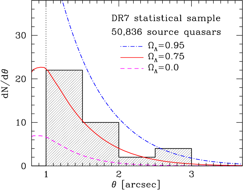
Figure 1: The histogram shows the image separation distribution of the strong lenses in the statistical lens sample used for our cosmological analyses. The subsample contains 19 lenses selected out of 50,836 source quasars, as summarized in Table The Sloan Digital Sky Survey Quasar Lens Search. VI. Constraints on Dark Energy and the Evolution of Massive Galaxies. Lines show the theoretical predictions for three different values of the cosmological constant $\Omega_{\Lambda}$ assuming a flat universe and no evolution of the galaxy velocity function. The vertical dotted line shows the $\theta_{\rm min}=1^{\prime\prime}$ lower limit for the image separations in the statistical lens sample.

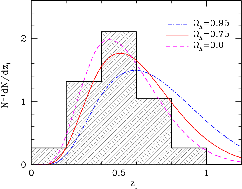
Figure 2: The histogram shows the normalized lens redshift distribution for our lens sample. Lines show theoretical predictions for three different cosmological models, as in Figure 1. For lenses with errors on the lens redshift (see Table The Sloan Digital Sky Survey Quasar Lens Search. VI. Constraints on Dark Energy and the Evolution of Massive Galaxies), we adopt the best estimated values in constructing the histogram.

We start with the simplest model, a flat universe where dark energy is described as a cosmological constant $\Omega_{\Lambda}$ (i.e., $w=-1$). This model has only one free parameter, $\Omega_{\Lambda}$. Before deriving constraints on $\Omega_{\Lambda}$, we compare the number distribution of lenses in our sample as a function of image separation with the model predictions, as shown in Figure 1. The total number of lenses is indeed sensitive to $\Omega_{\Lambda}$, and models with $\Omega_{\Lambda}\sim 0.8$ are broadly consistent with the observed number distribution. In Figure 2, we examine the normalized lens redshift distribution $N^{-1}dN/dz_{l}$. Here we see that the observed lens redshift distribution is more consistent with models with smaller $\Omega_{\Lambda}$ because of the relatively small number of lens galaxies at high lens redshifts.

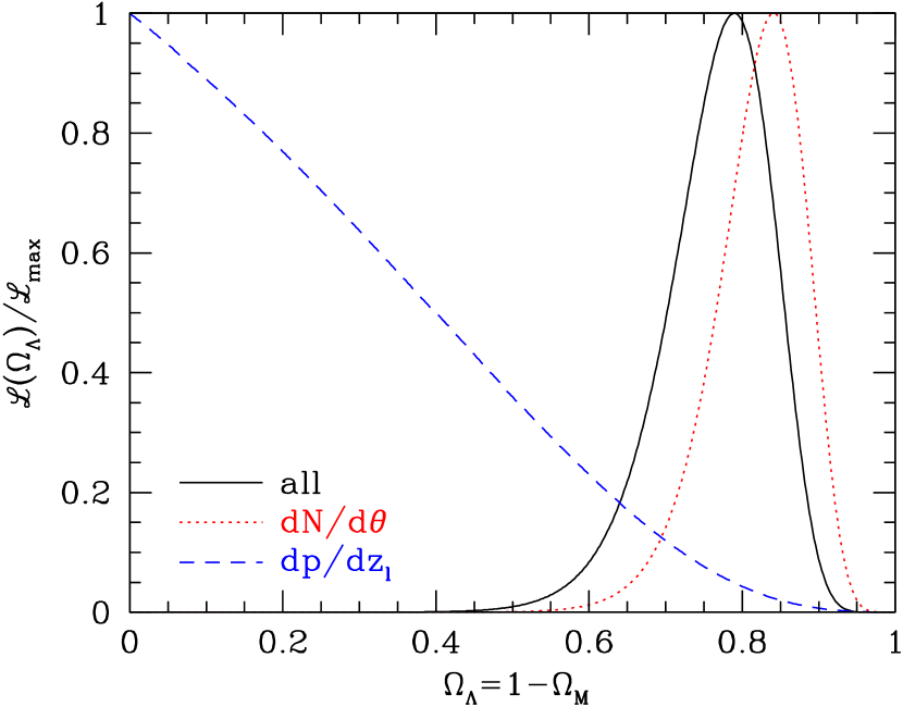
Figure 3: Likelihood distributions as a function of the cosmological constant $\Omega_{\Lambda}$ for flat universes. The dotted and dashed lines show the separate likelihood distributions for fitting the numbers and image separations alone (dotted) and lens redshifts alone (dashed).

We compute the likelihood of Equation (25) as a function of $\Omega_{\Lambda}$. The result shown in Figure 3 indicates that the SQLS DR7 sample constrains the cosmological constant to be $\Omega_{\Lambda}=0.79^{+0.06}_{-0.07}$, where the error indicates the statistical $1\sigma$ confidence limit. This is consistent with our previous results presented in Paper III and Inada et al. (2010, Paper IV). The model with $\Omega_{\Lambda}=0$ is rejected at $6\sigma$ level. Dark energy is detected at high significance by the quasar lens statistics.

If we divide the likelihood into the part contributed by the numbers and separations as compared to the lens redshifts, we see that there is some tension. The numbers and separations, which we used in our previous studies, favor somewhat higher $\Omega_{\Lambda}$ than the lens redshifts. In Figure 3, we show the resulting likelihoods as a function of $\Omega_{\Lambda}$ based only on the observed numbers and separations of lenses, as well as only on the lens redshift distribution. While the tension is only at about the $2\sigma$ level, this result may be suggestive of redshift evolution in the velocity function. This is one of the reasons that we consider simultaneous constraints on cosmological parameters and galaxy evolution in §5.

4.2 Non-Flat Models with a Cosmological Constant

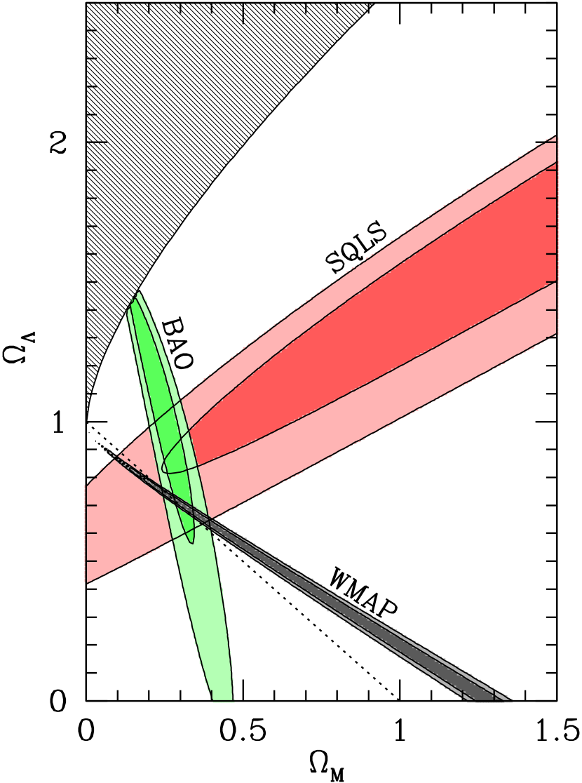
Figure 4: Constraints on $\Omega_{M}$ and $\Omega_{\Lambda}$ for the non-flat models with a cosmological constant. Contours show $1\sigma$ and $2\sigma$ confidence regions from the three different cosmological probes: SQLS strong lens statistics (this paper), baryon acoustic oscillation (BAO) measurements (Percival et al., 2010; Blake et al., 2011), and the CMB anisotropy from WMAP (Komatsu et al., 2011). The dotted line indicates a flat universe with $\Omega_{M}+\Omega_{\Lambda}=1$. The upper left shaded region indicates models with no big bang.

Next we relax the assumption of a flat universe, and consider cosmological constraints in the $\Omega_{M}$-$\Omega_{\Lambda}$ plane. Figure 4 shows the constraint from the SQLS DR7 using the full likelihood model. As already known (e.g., Kochanek, 1996; Chae et al., 2002), the degeneracy direction of lens constraints in the $\Omega_{M}$-$\Omega_{\Lambda}$ plane resembles that from Type Ia supernovae (see, e.g., Suzuki et al., 2012, for a recent result). We find that a cosmological constant is required at the $4\sigma$ level even for this non-flat case.

Because of different degeneracy directions, cosmological parameters are better constrained by combining several different cosmological probes. In this paper, we combine our constraints with either those from the baryon acoustic oscillation (BAO) measurement or from the cosmic microwave background (CMB). The former uses the baryon wiggle in the matter power spectrum as a standard ruler. We adopt results from the WiggleZ Dark Energy Survey (Blake et al., 2011), which measures the BAO scale at $z=0.6$, combined with BAO measurements in the SDSS luminous red galaxies at $z=0.2$ and $0.35$ (Percival et al., 2010). We consider the anisotropy measured by the Wilkinson Microwave Anisotropy Probe (WMAP) as the latter. Specifically we consider the seven-year WMAP result by Komatsu et al. (2011), and compute the likelihood for each cosmological parameter set by the so-called “distance prior” which encapsulates all the key information relevant for dark energy studies derived from the WMAP data. While our lensing constraints from the SQLS DR7 do not have any dependence on the Hubble constant, both the BAO and WMAP constraints are sensitive to the adopted Hubble constant. Thus, when adding the BAO and WMAP we always include the Hubble constant as an additional free parameter over which we marginalize to obtain constraints on parameters of interest.

These BAO and WMAP constraints are also shown in Figure 4. The best-fit parameters and $1\sigma$ statistical errors are $\Omega_{M}=0.28^{+0.03}_{-0.03}$ and $\Omega_{\Lambda}=0.88^{+0.09}_{-0.10}$ when the SQLS is combined with BAO, and $\Omega_{M}=0.20^{+0.08}_{-0.06}$ and $\Omega_{\Lambda}=0.78^{+0.05}_{-0.06}$ when combined with WMAP. The three constraints are complementary in the sense that their degeneracy directions are quite different from one another and the combined constraints give considerably stronger constraints in the $\Omega_{M}$-$\Omega_{\Lambda}$ plane than any of the individual constraints. That our lensing constraints are consistent with both the BAO and WMAP constraints is an important cross check of the current standard cosmological model.

4.3 Flat Dark Energy Models

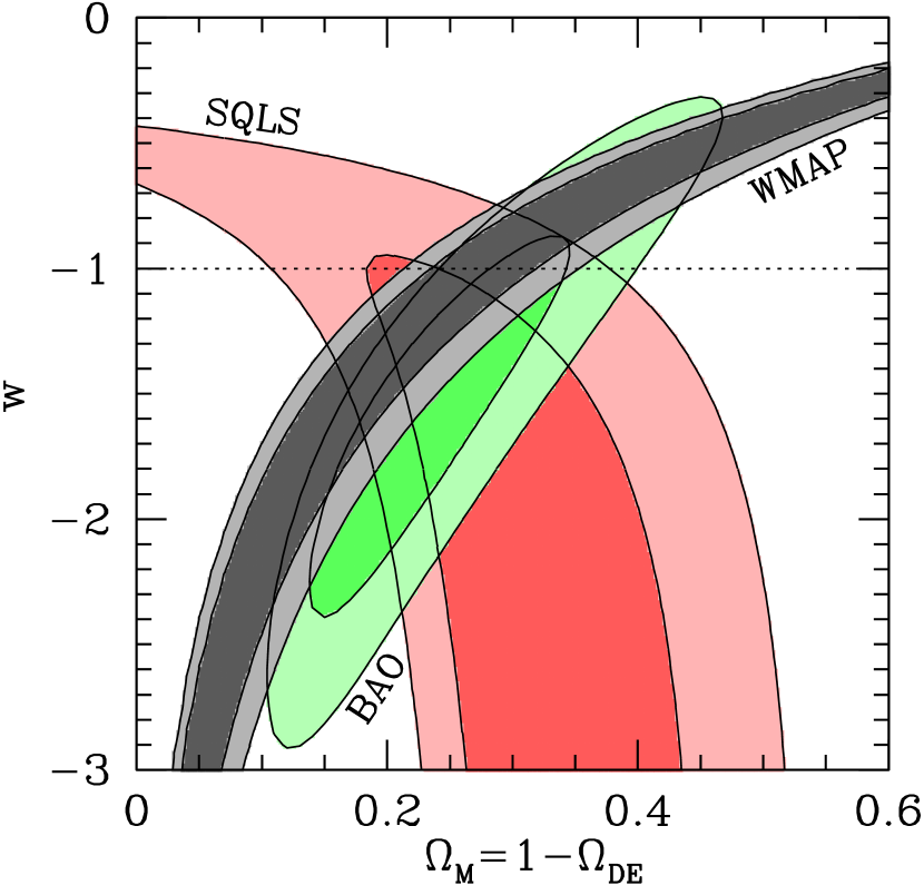
Figure 5: Constraints on $\Omega_{M}=1-\Omega_{\rm DE}$ and $w$ for the flat dark energy models. As in Figure 4, the $1\sigma$ and $2\sigma$ constraints from the three different cosmological probes are shown by contours. The horizontal dotted line indicates a cosmological constant with $w=-1$.

Next we consider flat models where the dark energy equation of state $w$ is allowed to vary. This model is parametrized by $\Omega_{M}$($=1-\Omega_{\rm DE}$) and $w$. Figure 5 shows constraints from the SQLS DR7 as well as those from BAO and WMAP. The degeneracy direction of our lensing constraint in this plane is again similar to that of Type Ia supernovae, and hence is complementary to the BAO and WMAP constraints. The combination of these constraints suggests a cosmological model with $\Omega_{M}\sim 0.3$ and $w\sim-1$.

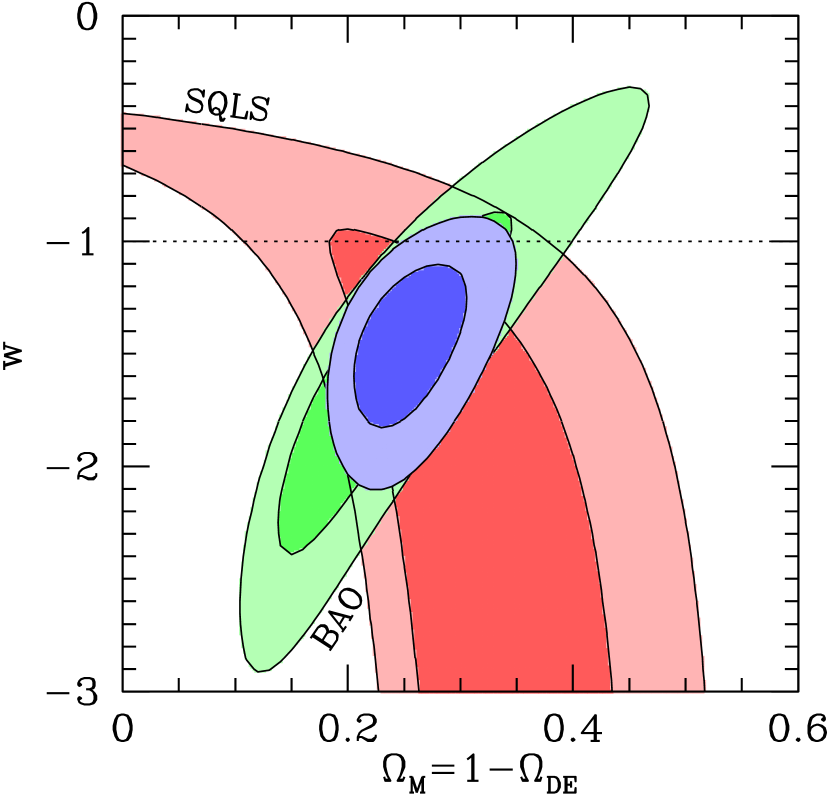
Figure 6: Similar to Figure 5, but with constraints only from the SQLS DR7 and BAO. The innermost contours show the combined constraint.

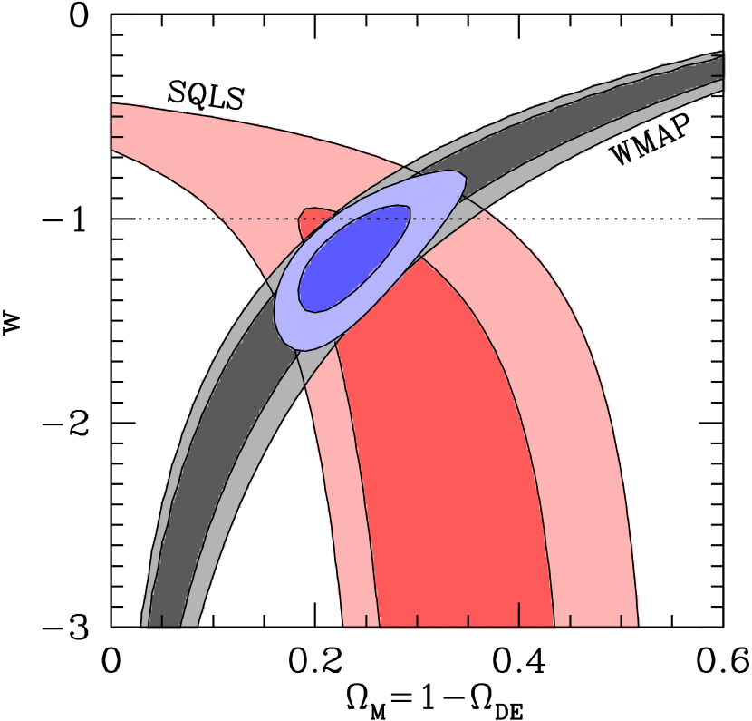
Figure 7: Similar to Figure 5, but with constraints only from the SQLS DR7 and WMAP. The innermost contours show the combined constraint.

We also show how $\Omega_{M}$ and $w$ are constrained when the lensing information is combined with either the BAO or WMAP result in Figure 6 and Figure 7, respectively. For the former case, the resulting constraints are $\Omega_{M}=0.25^{+0.03}_{-0.03}$ and $w=-1.44^{+0.22}_{-0.25}$, and for the latter case $\Omega_{M}=0.23^{+0.04}_{-0.03}$ and $w=-1.19^{+0.17}_{-0.17}$. In both cases, $\Omega_{M}$ and $w$ are reasonably well constrained thanks to the different degeneracy directions of the tests.

4.4 Systematic Errors

Thus far we have considered only statistical errors. Our model involves several uncertainties and assumptions which act as systematic errors in our cosmological analysis. Here we estimate these systematic errors in a similar way as done in Paper III. Specifically we consider the following sources of systematic errors.

• We computed the dynamical normalization $\lambda(e)$ in Equation (4) assuming galaxies consist of oblate and prolate populations with equal fractions $f_{\rm obl}=0.5$. As in Paper III, we change the fraction by $\pm 0.25$ to estimate the uncertainty associated with this assumption.

• The ellipticity distribution of lens galaxies is assumed to be a truncated Gaussian with a peak $\bar{e}=0.25$ and a width $\sigma_{e}=0.2$. We shift the peak $\bar{e}$ by $\pm 0.1$ without changing the dispersion in order to see how the ellipticity distribution affects the cosmological results.

• We included the line-of-sight convergence $\kappa_{\rm ext}$ and shear $\gamma_{\rm ext}$ using the PDFs derived from ray-tracing of $N$-body simulations (Takahashi et al., 2011) for a fixed source redshift of $z_{s}=2$. We change the assumed redshift by $\pm 1$ to estimate the systematic error.

• The faint end slope of the quasar luminosity function in Equation (14) is needed for computing the magnification bias, yet current measurements of the slope are fairly uncertain. Considering results of measurements on the quasar luminosity function (e.g., Hopkins et al., 2007), we change the faint end slope $\beta_{\rm l}$ by $\pm 0.1$ while fixing the other parameters of the quasar luminosity functions. While the range of $\beta_{\rm l}$ considered here is smaller than what was adopted in Paper III, it is still much larger than the measurement uncertainty reported in Croom et al. (2009).

• The velocity function given by Equation (10) is another important source of systematic error. While we adopted the velocity function measurement in the SDSS by Bernardi et al. (2010) as our fiducial model, we investigate how the cosmological results are altered by adopting the velocity function measurement by Chae (2010). The specific forms of both the velocity functions were given in §3.2.

• While we made the assumption that the velocity function does not evolve with redshift, i.e., $\nu_{n}=0$ and $\nu_{\sigma}=0$ in Equations (12) and (13), respectively, we check the effect of redshift evolution by adopting the evolution of $\nu_{n}=-0.229$ and $\nu_{\sigma}=-0.01$ predicted by the semi-analytic model of Kang et al. (2005). Note that we will explore the effect of letting $\nu_{n}$ and $\nu_{\sigma}$ be free parameters in § 5.

• As discussed in Paper III, the condition $i_{\rm QSO}-i_{\rm gal}<0$ is arbitrary. To estimate the systematic error, we shift the condition to $i_{\rm QSO}-i_{\rm gal}<\pm 0.25$, within which the lens sample used for the statistics does not change.

In Table 2, we show the contribution of each of these systematic errors to the systematic error on $\Omega_{\Lambda}$ for the flat models with a cosmological constant. We find that the largest sources of systemic error are the dynamical normalization $f_{\rm obl}$ and the velocity function $dn/d\sigma_{v}$, followed by the faint end slope of the quasar luminosity function. The finding is consistent with the earlier results in Paper III. The resulting final constraint on $\Omega_{\Lambda}$ from the SQLS alone including the systematic error is $\Omega_{\Lambda}=0.79^{+0.06}_{-0.07}({\rm stat.})^{+0.06}_{-0.06}({\rm syst.})$. Table 3 summarizes the cosmological constraints for the three cases studied above, including our estimates of systematic errors. All the results remain consistent with the current standard cosmological model ($\Omega_{M}\sim 0.3$, $\Omega_{\rm DE}\sim 0.7$, and $w\sim-1$).

5 Evolution of the Velocity Function

Thus far we have concentrated on the constraints on cosmological parameters from the statistics of lensed quasars. However, the lensing statistics also allow us to study the evolution and structure of the galaxies that act as lenses. In particular, the lens statistics serve as a useful probe of the velocity function of massive galaxies at intermediate redshifts, $0.2\lesssim z\lesssim 1$, which are difficult to observe directly. Indeed, the analysis in §4.4 suggests that redshift evolution of the velocity function is one of the most significant sources of systematic error. Here we relax the assumption about the absence of redshift evolution in the velocity function, and investigate redshift evolution parametrized by $\nu_{n}$ (Equation (12)) and $\nu_{\sigma}$ (Equation (13)). Unlike previous studies, however, we still allow cosmological parameters to vary and consider simultaneous constraints on the galaxy evolution and cosmological parameters with the help of external cosmological probes such as BAO and WMAP.

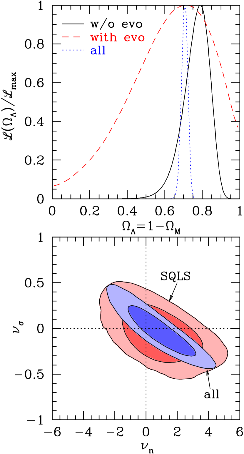
Figure 8: Simultaneous constraints on cosmological parameters and redshift evolution of the velocity function of galaxies in the flat models with a cosmological constant. Upper: Likelihood distributions as a function of cosmological constant $\Omega_{\Lambda}$. The solid line shows the likelihood from the SQLS alone with no redshift evolution as in Figure 3. The dashed line is the likelihood from the SQLS alone after marginalizing over the evolution parameters $\nu_{n}$ and $\nu_{\sigma}$. The dotted line is the likelihood distribution marginalizing over $\nu_{n}$ and $\nu_{\sigma}$ when the SQLS result is combined with the BAO and WMAP constraints. Lower: Constraints on redshift evolution in the $\nu_{n}$-$\nu_{\sigma}$ plane after marginalizing over $\Omega_{\Lambda}$. The outer contours are from the SQLS only, and the inner contours show the combined constraints from SQLS, BAO, and WMAP. Dotted lines in the lower panel indicate no redshift evolution ($\nu_{n}=0$ and $\nu_{\sigma}=0$).

First we consider the flat models with a cosmological constant. With the two additional parameters $\nu_{n}$ and $\nu_{\sigma}$, this model now has three parameters. The results using SQLS alone are shown in Figure 8. We find that a cosmological constant is still required even after the evolution parameters are left as free parameters and are fully marginalized over. Specifically, the cosmological constant is constrained to be $\Omega_{\Lambda}=0.71^{+0.20}_{-0.25}({\rm stat.}){}^{+0.12}_{-0.10}({\rm syst.})$ from the SQLS alone, which is consistent with the result assuming no redshift evolution of the velocity function shown in §4.1. The model without cosmological constant ($\Omega_{\Lambda}=0$) is still inconsistent with the data at more than $2\sigma$. The constraint projected in the $\nu_{n}$-$\nu_{\sigma}$ plane also indicates that the SQLS data are consistent with the no-redshift-evolution case ($\nu_{n}=\nu_{\sigma}=0$) at $1\sigma$. Also note that the most degenerate direction in the evolution parameters roughly corresponds to no evolution in the lensing optical depth. The additional constraints from BAO and WMAP, which significantly improve the constraint on $\Omega_{\Lambda}$, similarly improve the constraints in the $\nu_{n}$-$\nu_{\sigma}$ plane. With these additional constraints, results are still consistent with the no-redshift-evolution case. Specifically, the measured values of the two parameters are $\nu_{n}=1.06^{+1.36}_{-1.39}({\rm stat.}){}^{+0.33}_{-0.64}({\rm syst.})$ and $\nu_{\sigma}=-0.05^{+0.19}_{-0.16}({\rm stat.}){}^{+0.03}_{-0.03}({\rm syst.})$ when all three constraints are combined. The systematic errors are estimated in the same way as in §4.4, including the sources of the systematic error other than redshift evolution of the velocity function.

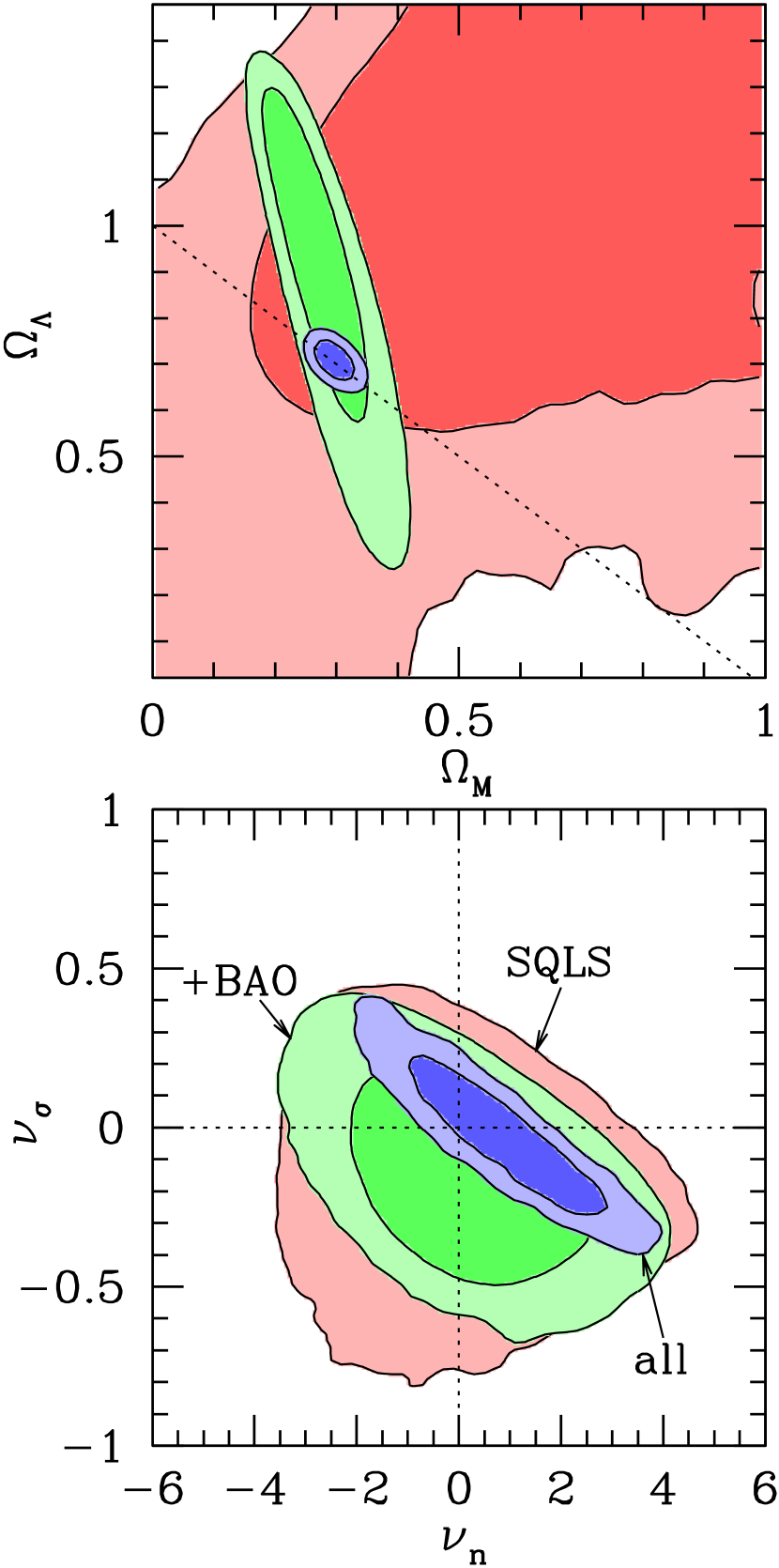
Figure 9: Simultaneous constraints on cosmological parameters and redshift evolution of the velocity function of galaxies in the non-flat models with a cosmological constant. The upper panel shows constraints in the $\Omega_{M}$-$\Omega_{\Lambda}$ plane after marginalizing over the evolution parameters $\nu_{n}$ and $\nu_{\sigma}$. The dotted line is a flat universe with $\Omega_{M}+\Omega_{\Lambda}=1$. Lower panel shows constraints in the $\nu_{n}$-$\nu_{\sigma}$ after marginalizing over the cosmological parameters. In both panels, from outer to inner contours, we show constraints from the SQLS alone, SQLS plus BAO, and the combination of all three probes (SQLS+BAO+WMAP), respectively. Dotted lines in the lower panel indicate no redshift evolution ($\nu_{n}=0$ and $\nu_{\sigma}=0$).

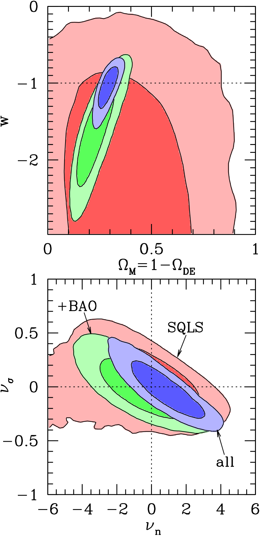
Figure 10: As in Figure 9, but for flat dark energy models with $w$ as a free parameter.

We conduct similar analyses of the simultaneous constraints in the non-flat models with a cosmological constant and in the flat dark energy models. The results, shown in Figures 9 and 10, indicate that the cosmological constraints from SQLS become much weaker when we allow the evolution parameters to vary, although some useful constraints are still obtained. For instance, in the non-flat cosmological constant case, non-zero $\Omega_{\Lambda}$ is again preferred at about $2\sigma$. On the other hand, the evolution parameters are constrained reasonably well even after marginalizing over cosmological parameters. In all the cases, the SQLS data are consistent with no redshift evolution, which supports early ($z\gtrsim 1$) formation and passive evolution of massive early-type galaxies. We give a summary of the constraints in Table 4. Note that systematic errors on the cosmological parameters appear smaller than in Table 3, because of weaker cosmological constraints from the SQLS after marginalizing over the evolution parameters.

Our non-detection of redshift evolution of the velocity function is consistent with earlier results by Mao & Kochanek (1994), Ofek et al. (2003), Chae & Mao (2003), Capelo & Natarajan (2007), and Matsumoto & Futamase (2008), although we believe our result is more robust given the carefully controlled lens sample from the SQLS and the exploration of the degeneracy with cosmological parameters. On the other hand, Chae (2010) reported that the lens data imply redshift evolution of the velocity function once a more complicated model is adopted for the evolution. To check this result, we consider the evolution of the shape of the velocity function by replacing $\alpha$ and $\beta$ in Equation (10) as Chae (2010) has suggested,

$$\alpha\rightarrow\alpha\left(1+k_{\beta}\frac{z}{1+z}\right),$$ (28)

$$\beta\rightarrow\beta\left(1+k_{\beta}\frac{z}{1+z}\right).$$ (29)

These additional parameterizations lead to differential redshift evolution in the number density of galaxies with different velocity dispersions. In particular, redshift evolution naively expected from the redshift dependence of the halo mass function, which predicts stronger redshift evolution for larger velocity dispersions (Mitchell et al., 2005; Matsumoto & Futamase, 2008), can well be described by this parametrization (Chae, 2010).

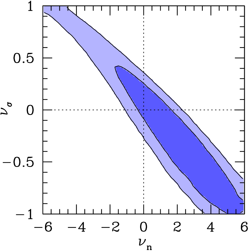
Figure 11: Constraints on redshift evolution of the velocity function. Here we include the additional parameter $k_{\beta}$ which describes redshift evolution of the shape of the velocity function as proposed by Chae (2010). We consider the flat models with a cosmological constant. The SQLS constraint is combined with BAO and WMAP. We show constraints in the $\nu_{n}$-$\nu_{\sigma}$ after marginalizing over the other parameters $\Omega_{\Lambda}$ and $k_{\beta}$. Dotted lines in the lower panel indicate no redshift evolution ($\nu_{n}=0$ and $\nu_{\sigma}=0$). The marginalized constraint on $k_{\beta}$ is $k_{\beta}=-0.35^{+0.67}_{-0.35}$.

Figure 11 shows constraints in the $\nu_{n}$-$\nu_{\sigma}$ plane in the flat models with a cosmological constant using all three cosmological constraints and marginalizing over the additional evolution parameter $k_{\beta}$ as well as the cosmological constant $\Omega_{\Lambda}$. We find no redshift evolution even in this case. The constraints on the individual evolution parameters are $\nu_{n}=2.47^{+2.27}_{-2.77}$, $\nu_{\sigma}=-0.35^{+0.52}_{-0.49}$, and $k_{\beta}=-0.35^{+0.67}_{-0.35}$ (statistical errors only), which are fully consistent with the fiducial no-redshift-evolution case of $\nu_{n}=\nu_{\sigma}=k_{\beta}=0$. Our different conclusion might be due to the fact that our source quasar sample is restricted to $z_{s}<2.2$ and therefore probes relatively low lens redshifts of $z_{l}\lesssim 1$, whereas the lens sample used by Chae (2010) extends to lens redshifts of $z_{l}>1$. On the other hand, our SQLS sample is more complete and has a better understood selection function than the somewhat heterogeneous, incomplete sample of source and lens redshifts adopted by Chae (2010).

6 Discussions

6.1 Comparisons with Other Studies on Galaxy Evolution

While our results are consistent with no evolution, the constraints are relatively weak. In the $\nu_{n}$-$\nu_{\sigma}$ plane, the evolution is roughly constrained to keep the lensing optical depth ($\propto\phi_{*}\sigma_{*}^{4}$) constant while weakly constraining the orthogonal combination. Studies of galaxy evolution have typically found significant number and mass evolution in the early-type population from $z=0$ to $1$ with a decline in the abundance of early-type galaxies by roughly a factor of $2$ by $z=1$ (e.g., Faber et al., 2007; Brown et al., 2007), which corresponds to $\nu_{n}\simeq-1$. This change in number is consistent with our results, but it also requires an increase in the characteristic velocity dispersion of 20% (i.e., $\nu_{\sigma}=0.25$). For the numbers to decline, the mean mass as indicated by the velocity dispersion has to increase. Eliminating this degeneracy requires samples of lenses large enough to cleanly measure the evolution of the average image separation with redshift (see §6.2).

Our results on the evolution in the velocity function can also be compared with recent evolution measurements in the stellar mass function. For instance, from the examination of galaxy populations at $z\sim 1-2$ it has been shown that the stellar mass function of galaxies indeed evolves from $z=0$ to $1$, though the mass dependence on the form of redshift evolution has yet to be fully clarified (e.g., Ilbert et al., 2010; Matsuoka & Kawara, 2010; Brammer et al., 2011). These studies showed that the number density of galaxies for a given stellar mass range can evolve by a factor of $\sim 2$ from $z=0$ to $1$, which is in fact compatible with our results given the large errors on the evolution parameters for our lensing analysis. While the direct evolution measurement of the velocity function is very challenging, Bezanson et al. (2011) has recently measured the evolution of the velocity function from $z=0$ to $1.5$ by taking advantage of a scaling relation between velocity dispersion, stellar mass, and galaxy structural properties, and found weak redshift evolution up to $z\sim 1$, which is consistent with our result.

6.2 Relation between Velocity Dispersion and Image Separation

Another possible source of uncertainties inherent to our analysis is the relation between velocity dispersions and image separations. While this uncertainty is partly taken into account in our analysis via the systematic error from the dynamical normalization, the true uncertainties can potentially be larger given complexities such as velocity anisotropies and the detailed luminosity profiles of galaxies. However, with a large number of lenses we can in principle determine the relation from the data, because the ensemble average of image separations is given by $\langle\theta\rangle\propto\sigma_{*}^{2}$ with a proportionality factor that is almost independent of cosmological parameters (see Kochanek, 1993, 1996).

To explore the possibility of calibrating the relation between velocity dispersions and image separations from the lensing data, we consider a simple parametric model in which the Einstein radius given by Equation (5) is modified to be

$$\theta_{\rm E}=(1+\xi)^{2}4\pi\left(\frac{\sigma_{v}}{c}\right)^{2}\frac{D_{\rm ls}}{D_{\rm os}},$$ (30)

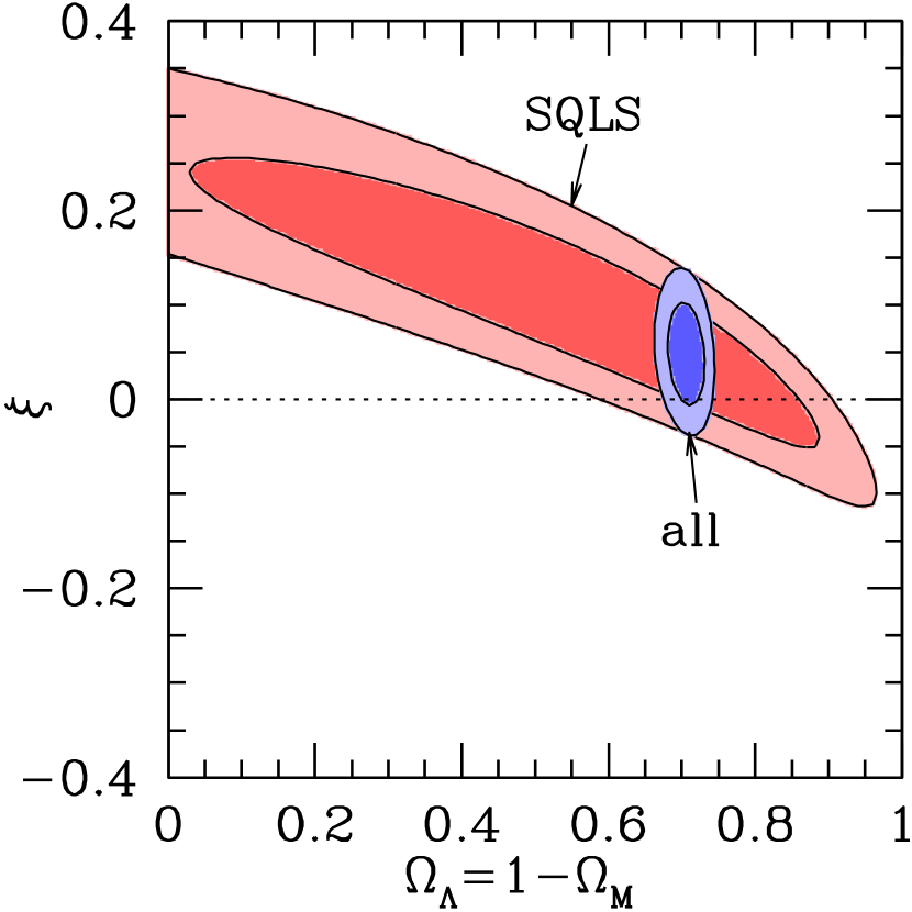
Figure 12: Constraints on the cosmological constant $\Omega_{\Lambda}$ and the parameter $\xi$ in Equation (30) that parametrizes the relation between velocity dispersions and image separations, for flat models with a cosmological constant. Outer and inner contours show constraints from the SQLS alone and from the combination of all three probes (SQLS+BAO+WMAP), respectively. The horizontal dotted line indicates the fiducial value $\xi=0$ assumed in the paper.

where the parameter $\xi$ parametrizes the relation such that $\xi=0$ if the velocity dispersion exactly matches the one used for our SIE models. We consider the flat models with a cosmological constant, and obtain simultaneous constraints on $\Omega_{\Lambda}$ and $\xi$. The result, shown in Figure 12, indicates that constraints on $\xi$ from the SQLS are degenerate with $\Omega_{\Lambda}$. The marginalized constraints on each parameter are $\xi=0.08^{+0.10}_{-0.09}$ and $\Omega_{\Lambda}=0.62^{+0.20}_{-0.33}$ (statistical errors only). Thus the cosmological constraints become much weaker, although models with a significant cosmological constant are still preferred. If we combine all three cosmological constraints, the resulting constraint is $\xi=0.05^{+0.03}_{-0.03}$. The slightly positive value reflects the fact that lens statistics with $\xi=0$ favor slightly larger $\Omega_{\Lambda}$ than the best-fit values from BAO and WMAP, and that the observed mean image separation appears to be slightly higher than the models predict (see Figure 1). Models with $\xi=0$ are consistent with the data to better than $2\sigma$.

7 Conclusion

We have conducted a statistical analysis of the final sample of strongly lensed quasars from the SQLS (Paper V). A subsample of 19 lenses selected from 50,836 quasars has been used to derive constraints on various cosmological parameters as well as the redshift evolution of the velocity function of galaxies. We have derived cosmological constraints assuming no redshift evolution of the velocity function. For the flat models with a cosmological constant, we have found $\Omega_{\Lambda}=0.79^{+0.06}_{-0.07}({\rm stat.})^{+0.06}_{-0.06}({\rm syst.})$ from the SQLS alone, which is in concord with other cosmological constraints. The model with $\Omega_{\Lambda}=0$ is rejected at $6\sigma$ (statistical errors only), which represents a significant detection of dark energy independent of Type Ia supernovae or other cosmological probes. The systematic error is comparable to the $1\sigma$ statistical error, suggesting the importance of careful studies of the systematics for robust cosmological constraints from lens statistics. We have also derived constraints on non-flat models with a cosmological constant and flat dark energy models, by combining the SQLS results with independent constraints from BAO and WMAP, and obtained results consistent with other studies (e.g., Komatsu et al., 2011). These constraints are summarized in Table 3.

We have also derived simultaneous constraints on the cosmological parameters and redshift evolution of the velocity function. We parametrize redshift evolution by two parameters $\nu_{n}$ (Equation (12)) and $\nu_{\sigma}$ (Equation (13)). The SQLS data still prefer a dark energy dominated universe even after marginalizing over the evolution parameters, with $\Omega_{\Lambda}=0.71^{+0.20}_{-0.25}({\rm stat.}){}^{+0.12}_{-0.10}({\rm syst.})$ for the flat models with a cosmological constant. We have found no significant evidence for redshift evolution in the velocity function, for example $\nu_{n}=1.06^{+1.36}_{-1.39}({\rm stat.}){}^{+0.33}_{-0.64}({\rm syst.})$ and $\nu_{\sigma}=-0.05^{+0.19}_{-0.16}({\rm stat.}){}^{+0.03}_{-0.03}({\rm syst.})$, when the SQLS results are combined with BAO and WMAP in the flat models with a cosmological constant. We summarize the simultaneous constraints in Table 4. The results remain consistent with no redshift evolution even if we consider evolution in the shape of the velocity function. A cautionary note is that because of the relatively low-redshifts of our source quasars, the SQLS sample probes galaxy evolution only at $z\lesssim 1$. It is of great importance to extend the lens statistics like the SQLS to higher quasar redshifts in order to study the number evolution of massive galaxies further, as well as for better constraints on dark energy. Future wide-field surveys such as Pan-STARRS and Large Synoptic Survey Telescope will discover thousands of lensed quasars efficiently by taking advantage of time-domain information (Oguri & Marshall, 2010), which should be helpful for advancing such applications.

Table 1: DR7 Statistical Sample from Paper V

Object	$N_{\rm img}$	$z_{s}$	$z_{l}$	$i_{\rm PSF}$	$\theta_{\rm max}$	$I_{\rm QSO}$	$I_{\rm gal}$	Ref.
SDSS J0246$-$0825	2	1.686	0.723	17.76	1.09	17.80	20.78	1,2,3
SDSS J0746+4403	2	1.998	0.513	18.71	1.08	18.71	19.62	4,5
SDSS J0806+2006	2	1.538	0.573	18.89	1.49	18.43	20.16	2,6,7
SBS 0909+523	2	1.378	0.830	16.17	1.11	15.94	18.81	3,8,9
SDSS J0924+0219	4	1.523	0.394	18.12	1.81	18.40	19.36	3,9,10,11
FBQ0951+2635	2	1.246	0.260	17.24	1.10	16.54	19.66	2,3,12
SDSS J1001+5027	2	1.841	0.415	17.32	2.86	17.32	19.63	13,14
SDSS J1021+4913	2	1.720	0.451	18.99	1.14	18.85	19.82	14,15
SDSS J1055+4628	2	1.249	0.388	18.76	1.15	18.86	19.73	5,14
PG1115+080	4	1.735	0.311	15.97	2.43	16.40	18.91	3,16,17
SDSS J1206+4332	2	1.789	0.748	18.46	2.90	18.05	19.51	13
SDSS J1216+3529	2	2.013	$0.55\pm 0.05$	19.08	1.49	18.30	20.31	18
SDSS J1226$-$0006	2	1.126	0.517	18.23	1.26	18.67	19.71	3,19,20
SDSS J1313+5151	2	1.877	0.194	17.70	1.24	17.10	17.49	21
SDSS J1335+0118	2	1.571	0.440	17.54	1.63	17.17	19.40	3,20,22
SDSS J1353+1138	2	1.624	$0.25\pm 0.05$	16.47	1.41	16.36	17.80	6
SDSS J1405+0959	2	1.810	0.66	19.05	1.98	18.70	19.70	23,24
SDSS J1455+1447	2	1.424	$0.42\pm 0.1$	18.22	1.73	18.21	18.51	5
SDSS J1515+1511	2	2.054	0.742	18.05	1.95	17.53	20.02	23
Q0957+561	2	1.413	0.36	16.68	6.17	16.69	17.11	3,25,26
SDSS J1004+4112	5	1.740	0.68	18.82	14.72	18.44	18.82	3,27,28,29,30
SDSS J1251+2935	4	0.802	0.410	18.86	1.79	19.32	18.43	31
SDSS J1320+1644	2	1.502	0.899	18.88	8.59	18.36	21.59	32
SDSS J1330+1810	4	1.393	0.373	18.35	1.76	18.34	17.84	33
SDSS J1332+0347	2	1.438	0.191	17.89	1.14	18.57	18.06	34
SDSS J1524+4409	2	1.210	0.320	18.76	1.67	19.49	18.33	18

Note. — The subsample of 19 lenses above the horizontal solid line is used for the final statistical analysis. See text for details.

References. — (1) Inada et al. 2005b; (2) Eigenbrod et al. 2007; (3) CASTLES webpage (C. S. Kochanek et al., http://cfa-www.harvard.edu/castles/.); (4) Inada et al. 2007; (5) Kayo et al. 2010; (6) Inada et al. 2006; (7) Sluse et al. 2008; (8) Oscoz et al. 1997; (9) Lubin et al. 2000; (9) Inada et al. 2003a; (10) Ofek et al. 2007; (11) Eigenbrod et al. 2006a; (12) Schechter et al. 1998; (13) Oguri et al. 2005a; (14) Paper IV (15) Pindor et al. 2006; (16) Weymann et al. 1980; (17) Kundic et al. 1997; (18) Oguri et al. 2008b; (19) Paper II (20) Eigenbrod et al. 2006b; (21) Ofek et al. 2007; (22) Oguri et al. 2004a; (23) Inada et al., in preparation; (24) Jackson et al. 2012. (25) Walsh et al. 1979; (26) Young et al. 1980; (27) Inada et al. 2003b; (28) Oguri et al. 2004b; (29) Inada et al. 2005a; (30) Inada et al. 2008b; (31) Kayo et al. 2007; (32) C. E. Rusu et al., in preparation; (33) Oguri et al. 2008c; (34) Morokuma et al. 2007.

Table 2: Breakdown of Systematic Errors for the Flat Models with a Cosmological Constant

Source	Error on $\Omega_{\Lambda}$
$f_{\rm obl}\rightarrow\pm 0.25$	${}^{+0.037}_{-0.032}$
$\bar{e}\rightarrow\pm 0.1$	${}^{+0.000}_{-0.006}$
$z_{s}$ for $\kappa_{\rm ext}$ and $\gamma_{\rm ext}$ $\rightarrow\pm 1$	${}^{+0.003}_{-0.000}$
$\beta_{\rm l}\rightarrow\pm 0.1$	${}^{+0.019}_{-0.018}$
Different $dn/d\sigma_{v}$	${}^{+0.000}_{-0.046}$
$dn/d\sigma_{v}$ evolution	${}^{+0.033}_{-0.000}$
$i_{\rm QSO}-i_{\rm gal}\rightarrow\pm 0.25$	${}^{+0.019}_{-0.011}$
Total	${}^{+0.057}_{-0.060}$

Note. — The total errors are estimated from the quadrature sum of all the systematic errors.

Table 3: Constraints on Cosmological Parameters

Model	Data	$\Omega_{M}$	$\Omega_{\rm DE}$	$w$
flat $\Omega_{\Lambda}$	SQLS	$\equiv 1-\Omega_{\Lambda}$	$0.79^{+0.06}_{-0.07}{}^{+0.06}_{-0.06}$	$\equiv-1$
non-flat $\Omega_{\Lambda}$	SQLS+BAO	$0.28^{+0.03}_{-0.03}{}^{+0.02}_{-0.02}$	$0.88^{+0.09}_{-0.10}{}^{+0.07}_{-0.09}$	$\equiv-1$
non-flat $\Omega_{\Lambda}$	SQLS+WMAP	$0.20^{+0.08}_{-0.06}{}^{+0.07}_{-0.07}$	$0.78^{+0.05}_{-0.06}{}^{+0.05}_{-0.05}$	$\equiv-1$
non-flat $\Omega_{\Lambda}$	SQLS+BAO+WMAP	$0.29^{+0.02}_{-0.02}{}^{+0.00}_{-0.00}$	$0.71^{+0.02}_{-0.02}{}^{+0.00}_{-0.00}$	$\equiv-1$
flat $\Omega_{\rm DE}$	SQLS+BAO	$0.25^{+0.03}_{-0.03}{}^{+0.03}_{-0.02}$	$\equiv 1-\Omega_{M}$	$-1.44^{+0.22}_{-0.25}{}^{+0.17}_{-0.18}$
flat $\Omega_{\rm DE}$	SQLS+WMAP	$0.23^{+0.04}_{-0.03}{}^{+0.03}_{-0.03}$	$\equiv 1-\Omega_{M}$	$-1.19^{+0.17}_{-0.17}{}^{+0.14}_{-0.15}$
flat $\Omega_{\rm DE}$	SQLS+BAO+WMAP	$0.28^{+0.02}_{-0.02}{}^{+0.01}_{-0.01}$	$\equiv 1-\Omega_{M}$	$-1.11^{+0.14}_{-0.17}{}^{+0.08}_{-0.10}$

Note. — The parameter values are followed by their statistical and systematic uncertainties, respectively. See the last paragraph of § 1 for the definitions of cosmological parameters.

Table 4: Constraints on Cosmological Parameters and the Redshift Evolution of the Velocity Function

Model	Data	$\Omega_{M}$	$\Omega_{\rm DE}$	$w$	$\nu_{n}$	$\nu_{\sigma}$
flat $\Omega_{\Lambda}$	SQLS	$\equiv 1-\Omega_{\Lambda}$	$0.71^{+0.20}_{-0.25}{}^{+0.12}_{-0.10}$	$\equiv-1$	$1.07^{+1.61}_{-1.64}{}^{+0.27}_{-0.82}$	$-0.05^{+0.20}_{-0.20}{}^{+0.04}_{-0.05}$
flat $\Omega_{\Lambda}$	SQLS+BAO	$\equiv 1-\Omega_{\Lambda}$	$0.69^{+0.03}_{-0.04}{}^{+0.00}_{-0.00}$	$\equiv-1$	$1.15^{+1.36}_{-1.43}{}^{+0.33}_{-0.72}$	$-0.05^{+0.19}_{-0.16}{}^{+0.03}_{-0.03}$
flat $\Omega_{\Lambda}$	SQLS+WMAP	$\equiv 1-\Omega_{\Lambda}$	$0.73^{+0.02}_{-0.03}{}^{+0.00}_{-0.00}$	$\equiv-1$	$1.00^{+1.35}_{-1.41}{}^{+0.30}_{-0.63}$	$-0.06^{+0.19}_{-0.16}{}^{+0.04}_{-0.03}$
flat $\Omega_{\Lambda}$	SQLS+BAO+WMAP	$\equiv 1-\Omega_{\Lambda}$	$0.71^{+0.02}_{-0.02}{}^{+0.00}_{-0.00}$	$\equiv-1$	$1.06^{+1.36}_{-1.39}{}^{+0.33}_{-0.64}$	$-0.05^{+0.19}_{-0.16}{}^{+0.03}_{-0.03}$
non-flat $\Omega_{\Lambda}$	SQLS+BAO	$0.25^{+0.06}_{-0.05}{}^{+0.01}_{-0.01}$	$1.02^{+0.20}_{-0.28}{}^{+0.06}_{-0.03}$	$\equiv-1$	$0.15^{+1.61}_{-1.39}{}^{+0.20}_{-0.34}$	$-0.14^{+0.20}_{-0.23}{}^{+0.08}_{-0.02}$
non-flat $\Omega_{\Lambda}$	SQLS+WMAP	$0.32^{+0.11}_{-0.09}{}^{+0.04}_{-0.13}$	$0.69^{+0.07}_{-0.08}{}^{+0.10}_{-0.03}$	$\equiv-1$	$1.29^{+1.24}_{-1.62}{}^{+0.38}_{-0.66}$	$-0.06^{+0.21}_{-0.16}{}^{+0.02}_{-0.06}$
non-flat $\Omega_{\Lambda}$	SQLS+BAO+WMAP	$0.30^{+0.02}_{-0.02}{}^{+0.00}_{-0.00}$	$0.71^{+0.02}_{-0.01}{}^{+0.00}_{-0.00}$	$\equiv-1$	$1.06^{+1.22}_{-1.24}{}^{+0.32}_{-0.65}$	$-0.05^{+0.15}_{-0.16}{}^{+0.04}_{-0.03}$
flat $\Omega_{\rm DE}$	SQLS+BAO	$0.21^{+0.07}_{-0.05}{}^{+0.01}_{-0.01}$	$\equiv 1-\Omega_{M}$	$-1.70^{+0.45}_{-0.40}{}^{+0.05}_{-0.10}$	$-0.48^{+1.71}_{-1.56}{}^{+0.33}_{-0.29}$	$-0.04^{+0.19}_{-0.19}{}^{+0.04}_{-0.03}$
flat $\Omega_{\rm DE}$	SQLS+WMAP	$0.17^{+0.15}_{-0.06}{}^{+0.06}_{-0.05}$	$\equiv 1-\Omega_{M}$	$-1.51^{+0.69}_{-0.60}{}^{+0.34}_{-0.32}$	$-0.51^{+2.38}_{-2.18}{}^{+0.88}_{-0.80}$	$-0.07^{+0.17}_{-0.19}{}^{+0.04}_{-0.03}$
flat $\Omega_{\rm DE}$	SQLS+BAO+WMAP	$0.29^{+0.02}_{-0.03}{}^{+0.00}_{-0.01}$	$\equiv 1-\Omega_{M}$	$-1.01^{+0.14}_{-0.18}{}^{+0.03}_{-0.03}$	$1.06^{+1.18}_{-1.39}{}^{+0.28}_{-0.66}$	$-0.05^{+0.16}_{-0.14}{}^{+0.03}_{-0.02}$

Note. — The parameter values are followed by their statistical and systematic uncertainties, respectively. See the last paragraph of § 1 for the definition of cosmological parameters.

References

- Abazajian et al. (2003) Abazajian, K., et al. 2003, AJ, 126, 2081
- Abazajian et al. (2004) Abazajian, K., et al. 2004, AJ, 128, 502
- Abazajian et al. (2005) Abazajian, K., et al. 2005, AJ, 129, 1755
- Abazajian et al. (2009) Abazajian, K. N., et al. 2009, ApJS, 182, 543
- Adelman-McCarthy et al. (2006) Adelman-McCarthy, J. K., et al. 2006, ApJS, 162, 38
- Adelman-McCarthy et al. (2007) Adelman-McCarthy, J. K., et al. 2007, ApJS, 172, 634
- Adelman-McCarthy et al. (2008) Adelman-McCarthy, J. K., et al. 2008, ApJS, 175, 297
- Bernardi et al. (2003) Bernardi, M., et al. 2003, AJ, 125, 1849
- Bernardi et al. (2010) Bernardi, M., Shankar, F., Hyde, J. B., Mei, S., Marulli, F., & Sheth, R. K. 2010, MNRAS, 404, 2087
- Bezanson et al. (2011) Bezanson, R., et al. 2011, ApJ, 737, L31
- Blake et al. (2011) Blake C., et al., 2011, MNRAS, 415, 2892
- Blanton et al. (2003) Blanton, M. R., Lin, H., Lupton, R. H., Maley, F. M., Young, N., Zehavi, I., & Loveday, J. 2003, AJ, 125, 2276
- Brammer et al. (2011) Brammer, G. B., et al. 2011, ApJ, 739, 24
- Brown et al. (2007) Brown, M. J. I., et al. 2007, ApJ, 654, 858
- Browne et al. (2003) Browne, I. W. A., et al. 2003, MNRAS, 341, 13
- Cao & Zhu (2012) Cao, S., & Zhu, Z.-H. 2012, A&A, 538, A43
- Capelo & Natarajan (2007) Capelo, P. R., & Natarajan, P. 2007, New Journal of Physics, 9, 445
- Chae (2003) Chae, K.-H. 2003, MNRAS, 346, 746
- Chae (2007) Chae, K.-H. 2007, ApJ, 658, L71
- Chae (2010) Chae, K.-H. 2010, MNRAS, 402, 2031
- Chae & Mao (2003) Chae, K.-H., & Mao, S. 2003, ApJ, 599, L61
- Chae et al. (2002) Chae, K.-H., et al. 2002, Phys. Rev. Lett., 89, 151301
- Chiba & Yoshii (1999) Chiba, M., & Yoshii, Y. 1999, ApJ, 510, 42
- Choi et al. (2007) Choi, Y.-Y., Park, C., & Vogeley, M. S. 2007, ApJ, 658, 884
- Coleman et al. (1980) Coleman, G. D., Wu, C.-C., & Weedman, D. W. 1980, ApJS, 43, 393
- Croom et al. (2009) Croom, S. M., Richards, G. T., Shanks, T., et al. 2009, MNRAS, 399, 1755
- Dalal & Watson (2004) Dalal, N., & Watson, C. R. 2004, preprint (arXiv:astro-ph/0409483)
- Doi et al. (2010) Doi, M., et al. 2010, AJ, 139, 1628
- Eigenbrod et al. (2006a) Eigenbrod, A., Courbin, F., Dye, S., Meylan, G., Sluse, D., Vuissoz, C., & Magain, P. 2006a, A&A, 451, 747
- Eigenbrod et al. (2006b) Eigenbrod, A., Courbin, F., Meylan, G., Vuissoz, C., & Magain, P. 2006b, A&A, 451, 759
- Eigenbrod et al. (2007) Eigenbrod, A., Courbin, F., & Meylan, G. 2007, A&A, 465, 51
- Faber et al. (2007) Faber, S. M., et al. 2007, ApJ, 665, 265
- Falco et al. (1998) Falco, E. E., Kochanek, C. S., & Munoz, J. A. 1998, ApJ, 494, 47
- Fassnacht et al. (2011) Fassnacht, C. D., Koopmans, L. V. E., & Wong, K. C. 2011, MNRAS, 410, 2167
- Faure et al. (2009) Faure, C., et al. 2009, ApJ, 695, 1233
- Faure et al. (2011) Faure, C., et al. 2011, A&A, 529, A72
- Fukugita et al. (1990) Fukugita, M., Futamase, T., & Kasai, M. 1990, MNRAS, 246, 24
- Fukugita et al. (1992) Fukugita, M., Futamase, T., Kasai, M., & Turner, E. L. 1992, ApJ, 393, 3
- Fukugita et al. (1996) Fukugita, M., Ichikawa, T., Gunn, J. E., Doi, M., Shimasaku, K., & Schneider, D. P. 1996, AJ, 111, 1748
- Gunn et al. (1998) Gunn, J. E., et al. 1998, AJ, 116, 3040
- Gunn et al. (2006) Gunn, J. E., et al. 2006, AJ, 131, 2332
- Hogg et al. (2001) Hogg, D. W., Finkbeiner, D. P., Schlegel, D. J., & Gunn, J. E. 2001, AJ, 122, 2129
- Holder & Schechter (2003) Holder, G. P., & Schechter, P. L. 2003, ApJ, 589, 688
- Hopkins et al. (2007) Hopkins, P. F., Richards, G. T., & Hernquist, L. 2007, ApJ, 654, 731
- Ilbert et al. (2010) Ilbert, O., et al. 2010, ApJ, 709, 644
- Inada et al. (2003a) Inada, N., et al. 2003a, AJ, 126, 666
- Inada et al. (2003b) Inada, N., et al. 2003b, Nature, 426, 810
- Inada et al. (2005a) Inada, N., et al. 2005a, PASJ, 57, L7
- Inada et al. (2005b) Inada, N., et al. 2005b, AJ, 130, 1967
- Inada et al. (2006) Inada, N., et al. 2006, AJ, 131, 1934
- Inada et al. (2007) Inada, N., et al. 2007, AJ, 133, 206
- Inada et al. (2008a) Inada, N., et al. 2008a, AJ, 135, 496 (Paper II)
- Inada et al. (2008b) Inada, N., Oguri, M., Falco, E. E., Broadhurst, T. J., Ofek, E. O., Kochanek, C. S., Sharon, K., & Smith, G. P. 2008b, PASJ, 60, L27
- Inada et al. (2010) Inada, N., et al. 2010, AJ, 140, 403 (Paper IV)
- Inada et al. (2012) Inada, N., et al. 2012, AJ, in press, arXiv:1203.1087 (Paper V)
- Ivezić et al. (2004) Ivezić, Ž., et al. 2004, Astronomische Nachrichten, 325, 583
- Jackson et al. (2012) Jackson, N., Rampadarath, H., Ofek, E. O., Oguri, M., & Shin, M.-S. 2012, MNRAS, 419, 2014
- Kang et al. (2005) Kang, X., Jing, Y. P., Mo, H. J., Börner, G. 2005, ApJ, 631, 21
- Kayo et al. (2007) Kayo, I., et al. 2007, AJ, 134, 1515
- Kayo et al. (2010) Kayo, I., Inada, N., Oguri, M., Morokuma, T., Hall, P. B., Kochanek, C. S., & Schneider, D. P. 2010, AJ, 139, 1614
- Keeton & Kochanek (1998) Keeton, C. R., & Kochanek, C. S. 1998, ApJ, 495, 157
- Keeton et al. (1997) Keeton, C. R., Kochanek, C. S., & Seljak, U. 1997, ApJ, 482, 604
- Kochanek (1992) Kochanek, C. S. 1992, ApJ, 384, 1
- Kochanek (1993) Kochanek, C. S. 1993, ApJ, 419, 12
- Kochanek (1996) Kochanek, C. S. 1996, ApJ, 466, 638
- Komatsu et al. (2011) Komatsu, E., et al. 2011, ApJS, 192, 18
- Koopmans et al. (2006) Koopmans, L. V. E., Treu, T., Bolton, A. S., Burles, S., & Moustakas, L. A. 2006, ApJ, 649, 599
- Koopmans et al. (2009) Koopmans, L. V. E., et al. 2009, ApJ, 703, L51
- Kundic et al. (1997) Kundic, T., Cohen, J. G., Blandford, R. D., & Lubin, L. M. 1997, AJ, 114, 507
- Lubin et al. (2000) Lubin, L. M., Fassnacht, C. D., Readhead, A. C. S., Blandford, R. D., & Kundić, T. 2000, AJ, 119, 451
- Mao & Kochanek (1994) Mao, S. D., & Kochanek, C. S. 1994, MNRAS, 268, 569
- Maoz & Rix (1993) Maoz, D., & Rix, H.-W. 1993, ApJ, 416, 425
- Matsumoto & Futamase (2008) Matsumoto, A., & Futamase, T. 2008, MNRAS, 384, 843
- Matsuoka & Kawara (2010) Matsuoka Y., Kawara K., 2010, MNRAS, 405, 100
- Momcheva et al. (2006) Momcheva, I., Williams, K., Keeton, C., & Zabludoff, A. 2006, ApJ, 641, 169
- McKean et al. (2007) McKean, J. P., Browne, I. W. A., Jackson, N. J., Fassnacht, C. D., & Helbig, P. 2007, MNRAS, 377, 430
- Mitchell et al. (2005) Mitchell, J. L., Keeton, C. R., Frieman, J. A., & Sheth, R. K. 2005, ApJ, 622, 81
- Morokuma et al. (2007) Morokuma, T., et al. 2007, AJ, 133, 214
- Muñoz et al. (2003) Muñoz, J. A., Falco, E. E., Kochanek, C. S., Lehár, J., & Mediavilla, E. 2003, ApJ, 594, 684
- Myers et al. (2003) Myers, S. T., et al. 2003, MNRAS, 341, 1
- Ofek et al. (2003) Ofek, E. O., Rix, H.-W., & Maoz, D. 2003, MNRAS, 343, 639
- Ofek et al. (2007) Ofek, E. O., Oguri, M., Jackson, N., Inada, N., & Kayo, I. 2007, MNRAS, 382, 412
- Oguri (2010) Oguri, M. 2010, PASJ, 62, 1017
- Oguri & Marshall (2010) Oguri, M., & Marshall, P. J. 2010, MNRAS, 405, 2579
- Oguri et al. (2004a) Oguri, M., et al. 2004a, PASJ, 56, 399
- Oguri et al. (2004b) Oguri, M., et al. 2004b, ApJ, 605, 78
- Oguri et al. (2005a) Oguri, M., et al. 2005a, ApJ, 622, 106
- Oguri et al. (2005b) Oguri, M., Keeton, C. R., & Dalal, N. 2005b, MNRAS, 364, 1451
- Oguri et al. (2006) Oguri, M., et al. 2006, AJ, 132, 999 (Paper I)
- Oguri et al. (2008a) Oguri, M., et al. 2008a, AJ, 135, 512 (Paper III)
- Oguri et al. (2008b) Oguri, M., et al. 2008b, AJ, 135, 520
- Oguri et al. (2008c) Oguri, M., Inada, N., Blackburne, J. A., Shin, M.-S., Kayo, I., Strauss, M. A., Schneider, D. P., & York, D. G. 2008c, MNRAS, 391, 1973
- Oscoz et al. (1997) Oscoz, A., Serra-Ricart, M., Mediavilla, E., Buitrago, J., & Goicoechea, L. J. 1997, ApJ, 491, L7
- Padmanabhan et al. (2008) Padmanabhan, N., et al. 2008, ApJ, 674, 1217
- Percival et al. (2010) Percival, W. J., et al. 2010, MNRAS, 401, 2148
- Pier et al. (2003) Pier, J. R., Munn, J. A., Hindsley, R. B., Hennessy, G. S., Kent, S. M., Lupton, R. H., & Ivezić, Ž. 2003, AJ, 125, 1559
- Pindor et al. (2006) Pindor, B., et al. 2006, AJ, 131, 41
- Padilla & Strauss (2008) Padilla, N. D., & Strauss, M. A. 2008, MNRAS, 388, 1321
- Richards et al. (2002) Richards, G. T., et al. 2002, AJ, 123, 2945
- Richards et al. (2006) Richards, G. T., et al. 2006, AJ, 131, 2766
- Rusin & Kochanek (2005) Rusin, D., & Kochanek, C. S. 2005, ApJ, 623, 666
- Schechter et al. (1998) Schechter, P. L., Gregg, M. D., Becker, R. H., Helfand, D. J., & White, R. L. 1998, AJ, 115, 1371
- Schlegel et al. (1998) Schlegel, D. J., Finkbeiner, D. P., & Davis, M. 1998, ApJ, 500, 525
- Schneider et al. (2010) Schneider, D. P., et al. 2010, AJ, 139, 2360
- Sluse et al. (2008) Sluse, D., Courbin, F., Eigenbrod, A., & Meylan, G. 2008, A&A, 492, L39
- Smith et al. (2002) Smith, J. A., et al. 2002, AJ, 123, 2121
- Sonnenfeld et al. (2012) Sonnenfeld, A., et al. 2012, arXiv:1111.4215
- Stoughton et al. (2002) Stoughton, C., et al. 2002, AJ, 123, 485
- Suyu et al. (2010) Suyu, S. H., Marshall, P. J., Auger, M. W., Hilbert, S., Blandford, R. D., Koopmans, L. V. E., Fassnacht, C. D., & Treu, T. 2010, ApJ, 711, 201
- Suzuki et al. (2012) Suzuki, N., et al. 2012, ApJ, 746, 85
- Takahashi et al. (2011) Takahashi, R., Oguri, M., Sato, M., & Hamana, T. 2011, ApJ, 742, 15
- Treu et al. (2009) Treu, T., et al. 2009, ApJ, 690, 670
- Tucker et al. (2006) Tucker, D. L., et al. 2006, Astronomische Nachrichten, 327, 821
- Turner (1990) Turner, E. L. 1990, ApJ, 365, L43
- Turner et al. (1984) Turner, E. L., Ostriker, J. P., & Gott, J. R., III 1984, ApJ, 284, 1
- Vanden Berk et al. (2005) Vanden Berk, D. E., et al. 2005, AJ, 129, 2047
- Walsh et al. (1979) Walsh, D., Carswell, R. F., & Weymann, R. J. 1979, Nature, 279, 381
- Weymann et al. (1980) Weymann, R. J., et al. 1980, Nature, 285, 641
- York et al. (2000) York, D. G., et al. 2000, AJ, 120, 1579
- Young et al. (1980) Young, P., Gunn, J. E., Oke, J. B., Westphal, J. A., & Kristian, J. 1980, ApJ, 241, 507