Irregular singularities in Liouville theory
and Argyres-Douglas type gauge theories, I

Abstract

Motivated by problems arising in the study of N=2 supersymmetric gauge theories we introduce and study irregular singularities in two-dimensional conformal field theory, here Liouville theory. Irregular singularities are associated to representations of the Virasoro algebra in which a subset of the annihilation part of the algebra act diagonally. In this paper we define natural bases for the space of conformal blocks in the presence of irregular singularities, describe how to calculate their series expansions, and how such conformal blocks can be constructed by some delicate limiting procedure from ordinary conformal blocks. This leads us to a proposal for the structure functions appearing in the decomposition of physical correlation functions with irregular singularities into conformal blocks. Taken together, we get a precise prediction for the partition functions of some Argyres-Douglas type theories on $S^{4}$.

1 Introduction

In this paper we answer a question which arises from the interplay [AGT] of four-dimensional ${\cal N}=2$ gauge theory and two-dimensional CFT. In the gauge-theory language, the question can be stated as: how can we compute the $S^{4}$ partition function [P07] of an Argyres-Douglas theory [AD, APSW]? In the 2d CFT language, the question becomes: how can we compute Liouville theory correlation functions in the presence of an irregular vertex operator [G09b]? The equivalence of these two questions follows from two facts. First, the $S^{4}$ partition function of a certain class of $SU(2)$ gauge theories coincides with standard Liouville theory correlation functions. Second, a limiting procedure which defines Argyres-Douglas theories from $SU(2)$ gauge theories [GMN] has a simple interpretation as a collision limit in Liouville theory, which produces irregular vertex operators from the collision of several standard vertex operators.

The existence of a well-defined collision limit for Liouville theory correlation functions is far from obvious from a two-dimensional perspective. The connection to gauge theory is a crucial source of inspiration in defining the notion of irregular vertex operator in Liouville theory. Once we have a solid two-dimensional definition of our objective, the 2d CFT perspective is best suited for the actual calculation of the answer. The calculation proceeds in two stages. First, we define and compute a basis of conformal blocks with irregular singularities which has properties analogous to the standard BPZ conformal blocks [BPZ]. Then we identify a measure which combines holomorphic and anti-holomorphic conformal blocks into a well-defined Liouville theory correlation function. A posteriori, the various stages of the 2d CFT calculation can then be given an intuitive gauge-theory interpretation.

The relations between N=2 supersymmetric gauge theories and Liouville theory referred to above appear to be part of a larger story that has started unfolding, relating supersymmetric gauge theories, conformal field theories, (quantized) moduli spaces of flat connections, various integrable models and the geometric Langlands program, see [KW, GMN, NS, AT, T10, NRS] for an incomplete list of relevant references. A common theme in these developments are relations with the Hitchin integrable system and with moduli spaces of flat connections on Riemann surfaces. The consideration of irregular singularities appears to be a very natural generalization in this context. From this point of view it seemed overdue from this point of view to have a Liouville theory with irregular singularities.

This paper is meant to be the first of a series of papers on this subject. While we here focus on more algebraic aspects like the construction of the conformal blocks, subsequent publications will in particular discuss analogs of the modular transformations relating different bases for spaces of conformal blocks, and relations with a generalization of the quantum Teichmüller theory to cases with irregular singularities.

The structure of the paper mirrors this logical structure. In section 2 we define the notion of an irregular conformal block. In sections 3 and 5 we describe two different, natural ways to define the same BPZ-like basis of irregular conformal blocks and clarify the nature of collision limits. In section 6 we use the collision limit to derive the correct integration measure for a Liouville correlation function. Finally, in section 7 we provide the gauge theory interpretation of the various ingredients of the 2d CFT answer. We refer the reader to the introductory part of each section for further details.

While this paper was being written, reference [BMT] appeared which has partial overlap with the discussion in Sections 2 and 7.

Acknowledgements: The work of DG is supported in part by NSF grant NSF PHY-0969448 and in part by the Roger Dashen membership in the Institute for Advanced Study. Opinions and conclusions expressed here are those of the authors and do not necessarily reflect the views of funding agencies.

JT would like to thank the Institute for Advanced Study for where part of this work was carried out for hospitality.

2 Irregular singularities in conformal field theory

2.1 Irregular vectors

A primary field $\Psi_{\Delta}(z)$ in conformal field theory is defined by the operator product expansion

$$T(y)\Psi_{\Delta}(z)\,\sim\,\frac{\Delta}{(y-z)^{2}}+\frac{1}{y-z}\frac{\partial}{\partial z}\Psi_{\Delta}(z)\,,$$ (2.1)

which is closely related to the statement the the state $|\Delta\rangle$ created as

$$|\Delta\rangle\,:=\,\lim_{z\to 0}\Psi_{\Delta}(z)|0\rangle$$ (2.2)

satisfies the highest weight property

$$L_{n}|\Delta\rangle\,=\,0\,,\quad n>0\,,\qquad L_{0}|\Delta\rangle\,=\,\Delta\,|\Delta\rangle\,.$$ (2.3)

Interpreting the Virasoro generators $L_{n}$ with $n>0$ as generalizations of “annihilation” operators may lead one to consider analogs of the coherent states where some subset of the generators $L_{n}$ with $n>0$ acts diagonally as

$$L_{k}|\,I\,\rangle\,=\,\Lambda_{k}|\,I\,\rangle\,.$$ (2.4)

From a mathematical perspective one may regard such vectors as analogs of the so-called Whittaker vectors in the representation theory of real reductive groups.

The Virasoro algebra, in particular the relations $[L_{k},L_{k^{\prime}}]=(k-k^{\prime})L_{k+k^{\prime}}$ for $k,k^{\prime}\geq 0$, imply that $\Lambda_{k+k^{\prime}}=0$ if both $L_{k}$ and $L_{k^{\prime}}$ are contained in the set of generators which act diagonally as in (2.4). Based on this observation it is easy to see that the values of the indices $k$ for which the eigenvector property (2.4) can hold with $\Lambda_{k}\neq 0$ must be taken from one of the sets $\{n,n+1,\dots,2n\}$, where $n$ is a positive integer. We will say that $|I_{n}\rangle$ is an irregular vectors of order $n$ if it satisfies

$$L_{k}|\,I\,\rangle\,=\,\Lambda_{k}|\,I\,\rangle\,,\quad k=n,\dots,2n\,,$$ (2.5a)

$$L_{k}|\,I\,\rangle\,=\,0\,,\quad k>2n\,.$$ (2.5b)

The collection $\Lambda=\{\Lambda_{n},\dots,\Lambda_{2n}\}$ of eigenvalues parameterizes the irregular vectors of order $n$, which may be expressed by using the notation $|I_{n},\Lambda\rangle$.

The representation of the generators $L_{k}$, $k=0,\dots,n-1$, is severely restricted by the relations $[L_{k},L_{k^{\prime}}]=(k-k^{\prime})L_{k+k^{\prime}}$ for $k,k^{\prime}\geq 0$. A convenient way to satisfy these relations can be introduced by using the parameterization

$$\Lambda_{k}\,=\,((k+1)Q-2\alpha)c_{k}-\sum_{l=1}^{k-1}c_{l}c_{k-l}\,,\qquad k=n,\dots,2n\,.$$ (2.6)

This expresses the $n+1$ parameters $\Lambda=\{\Lambda_{n},\dots,\Lambda_{2n}\}$ in terms of the parameter $\alpha$ and the collection of parameters ${\mathbf{c}}=(c_{1},\dots,c_{n})$. It is then elementary to check that the definitions

$$L_{k}|\,I_{n}\,\rangle\,:=\,{\mathcal{L}}_{k}|\,I_{n}\,\rangle\,,\qquad\begin{aligned} &{\mathcal{L}}_{k}\equiv{\mathcal{L}}_{k}({\mathbf{c}},\alpha):=\Lambda_{k}+\sum_{l=k+1}^{n-1}(l-k)c_{l}\frac{\partial}{\partial c_{l-k}}\,,\\ &{\mathcal{L}}_{0}\equiv{\mathcal{L}}_{0}({\mathbf{c}},\alpha):=\alpha(Q-\alpha)+\sum_{k=1}^{n}k\,c_{k}\frac{\partial}{\partial c_{k}}\,,\end{aligned}$$ (2.7)

are compatible with the algebraic relations $[L_{k},L_{k^{\prime}}]=(k-k^{\prime})L_{k+k^{\prime}}$, where $k,k^{\prime}\geq 0$.

It will often be convenient to summarize the conditions (2.5) and (2.7) in the form

$$T_{>}(y)|\,I_{n}\,\rangle\,=\,\Biggl{[}\;\sum_{k=n}^{2n}\frac{\Lambda_{k}}{y^{k+2}}+\sum_{k=0}^{n-1}\frac{{\mathcal{L}}_{k}}{y^{k+2}}+\frac{1}{y}L_{-1}\,\Biggr{]}|\,I_{n}\,\rangle\,,$$ (2.8)

where $T_{>}(y):=\sum_{k\geq-1}y^{-n-2}L_{n}$. The formula (2.8) encodes the singular behavior of the energy-momentum tensor $T(y)$ in the vicinity of an irregular singularity at $y=0$.

A more invariant point of view is to regard the conditions (2.5b) as natural generalization of the highest weight conditions (2.3). The highest weigth condition (2.3) says that $|\Delta\rangle$ is fixed by the algebra of holomorphic vector fields ${{\mathsf{V}}{\mathsf{e}}{\mathsf{c}}{\mathsf{t}}}_{{\mathbb{D}}}$ on the unit disc ${\mathbb{D}}=\{z\in{\mathbb{C}};|z|<1\}$ with generators $L_{k}\simeq z^{k}(z\partial_{z}+\Delta(k+1))$, $k\geq 0$. The space of all vectors which satisfy (2.5b) must then be a representation of the truncated algebra ${{\mathsf{V}}{\mathsf{e}}{\mathsf{c}}{\mathsf{t}}}_{{\mathbb{D}}}^{(n)}$ of holomorphic vector fields on a disc which has generators $l_{k}$, $k=0,\dots,2n$ and relations

$$\begin{aligned} &[\,l_{k}\,,\,l_{k^{\prime}}\,]\,=\,(k-k^{\prime})l_{k+k^{\prime}}\,,\quad{\rm if}\;\;k+k^{\prime}\leq 2n\,,\\ &[\,l_{k}\,,l_{k^{\prime}}\,]\,=\,0\,,\quad{\rm if}\;\;k+k^{\prime}>2n\,,\end{aligned}\qquad 0\leq k,k^{\prime}\leq 2n\,.$$

The equations (2.5a), (2.6) and (2.7) define representations of ${{\mathsf{V}}{\mathsf{e}}{\mathsf{c}}{\mathsf{t}}}_{{\mathbb{D}}}^{(n)}$ on spaces of functions of the $n+1$ variables $\alpha$ and ${\mathbf{c}}=(c_{1},\dots,c_{n})$.

2.1.1 Comparison to free-field representation

Let us introduce the (left-moving) chiral free field $\varphi(z)$, with mode-expansion given by

$$\phi(z)=q-\alpha_{p}\log z+\sum_{k\neq 0}\frac{i}{n}a_{n}z^{-n}\,,\qquad\alpha_{p}:=ip+\frac{Q}{2}\,.$$ (2.9)

The modes are postulated to have the following commutation and hermiticity relations

$$[q,p]=\frac{i}{2},\quad\begin{aligned} q^{\dagger}=&q,\\ p^{\dagger}=&p,\end{aligned}\qquad[a_{n},a_{m}]=\frac{n}{2}\delta_{n+m},\quad a_{n}^{\dagger}=a_{-n},$$ (2.10)

which are realized in the Hilbert-space

$${\mathcal{H}}^{\rm\scriptscriptstyle F}_{\rm\scriptscriptstyle L}\;\equiv\;L^{2}({\mathbb{R}})\otimes{\mathcal{F}},$$ (2.11)

where ${\mathcal{F}}$ is the Fock-space generated by acting with the modes $a_{n}$, $n<0$ on the Fock-vacuum $\Omega$ that satisfies $a_{n}\Omega=0$, $n>0$. We will mainly work in a representation where $p$ is diagonal.

The action of the Virasoro algebra on ${\mathcal{H}}^{\rm\scriptscriptstyle F}_{\rm\scriptscriptstyle L}$ can be defined in terms of the generators $L_{n}\equiv L_{n}(p)$, where

$$L_{n}(p)\;= (2p+inQ)a_{n}+\sum_{k\neq 0,n}a_{k}a_{n-k},\qquad n\neq 0,$$ (2.12)

$$L_{0}(p)\;= p^{2}+\frac{Q^{2}}{4}+2\sum_{k>0}a_{-k}a_{k}.$$

Equations (2.12) yield a representation of the Virasoro algebra with central charge

$$c\;=\;1+6Q^{2}.$$ (2.13)

Let us consider coherent states $|{\mathbf{c}};\alpha\rangle^{(n)}$ that satisfy

$$\begin{aligned} &a_{k}\,|{\mathbf{c}};\alpha\rangle^{(n)}\,=\,-ic_{k}\,|{\mathbf{c}};\alpha\rangle^{(n)}\,,\\ &a_{k}\,|{\mathbf{c}};\alpha\rangle^{(n)}\,=\,0\,,\end{aligned}\qquad\begin{aligned} &{\rm for}\;\;0<k\leq n\,,\\ &{\rm for}\;\;k>n\,.\end{aligned}$$ (2.14)

It follows directly (2.14) that the coherent states $|{\mathbf{c}};\alpha\rangle^{(n)}$ represent a very special example of irregular vector of degree $n$ within the Fock space representation (2.12) of the Virasoro algebra. In a sense, the Ward identities for general irregular vectors are modeled on this specific example.

We will discuss in a later section 4 how to give a free-field description of more general irregular vectors by dressing such bare coherent state with screening charges.

2.1.2 Irregular modules

From a given irregular vector we may generate infinitely many other vectors by acting with the Virasoro generators. It will be useful for us to formalize the point of view that this leads to the definition of new types of Virasoro modules.

To this aim, let us first note that the space ${\rm DO}^{(n)}$ of algebraic differential operators in $n$ variables ${\mathbf{c}}=(c_{1},\dots,c_{n})$ is naturally a module for the subalgebra ${\rm Vir}_{+}$ isomorphic to ${{\mathsf{V}}{\mathsf{e}}{\mathsf{c}}{\mathsf{t}}}_{{\mathbb{D}}}$ generated by $L_{k}$, $k\geq 0$. Identifying the trivial differential operator $1$ with the irregular vector $I^{(n)}_{{\mathbf{c}};\alpha}$ corresponds to defining the action of ${\rm Vir}_{+}$ on ${\rm DO}^{(n)}$ via

$$L_{k}\cdot{\mathcal{D}}\,=\,{\mathcal{D}}\,{\mathcal{L}}_{k}({\mathbf{c}};\alpha)\,,\qquad\forall\;\,{\mathcal{D}}\in{\rm DO}^{(n)}\,.$$ (2.15)

From this representation of ${\rm Vir}_{+}$ one may then naturally induce a representation ${\mathcal{V}}_{{\mathbf{c}};\alpha}^{(n)}$ of the full Virasoro algebra. As a vector space ${\mathcal{V}}_{{\mathbf{c}};\alpha}^{(n)}$ is spanned by expressions of the form

$${\mathbb{L}}_{-I}\,{\mathcal{D}}\,:=\,L_{-k}^{l_{k}}\,L_{-(k-1)}^{l_{k-1}}\,\cdots\,L_{-1}^{l_{1}}\,{\mathcal{D}}\,,$$ (2.16)

where ${\mathcal{D}}$ is any element of a basis for ${\rm DO}^{(n)}$. The action of the Virasoro algebra is defined in the usual way: Writing

$$L_{k}\,{\mathbb{L}}_{-I}\,=\,\sum_{k^{\prime}=0}^{k}\sum_{I^{\prime}}R_{kk}^{II^{\prime}}\;{\mathbb{L}}_{-I^{\prime}}\,L_{k^{\prime}}\,,$$ (2.17)

with the help of the Virasoro algebra, we may apply (2.15) with $k$ replaced by $k^{\prime}$ to define the action of $L_{k}$ on any basis element of the form ${\mathbb{L}}_{-I}\,{\mathcal{D}}$.

Irregular vectors and the associated modules were recently discussed from a similar point of view in [FJK].

2.2 Irregular singularities from collision of primary fields

Further motivation for the definitions above can be obtained from the consideration of certain collision limits of usual primary fields. Let us consider vectors

$$|\,R_{n}(z)\,\rangle\,\,\equiv\,|R_{n}(z_{1},\dots,z_{n})\rangle:=\prod_{r=1}^{n+1}\Psi_{\Delta_{r}}(z_{r})|\,0\,\rangle\,,$$

that are created by acting with a product of primary fields $\Psi_{\Delta_{r}}(z_{r})$ on the vacuum $|0\rangle$. The vectors $|\,R_{n}(z)\,\rangle$ satisfy the conditions

$$L_{k}|\,R_{n}(z)\,\rangle\,=\,\sum_{r=1}^{n+1}z_{r}^{k}\left(z_{r}\frac{\partial}{\partial z_{r}}+\Delta_{r}(k+1)\right)|\,R_{n}(z)\,\rangle\,,\quad k\geq-1\,,$$ (2.18)

which are summarized in

$$T_{>}(y)|\,R_{n}(z)\,\rangle\,=\,\sum_{r=1}^{n+1}\left(\frac{\Delta_{\alpha_{r}}}{(y-z_{r})^{2}}+\frac{1}{y-z_{r}}\frac{\partial}{\partial z_{r}}\right)|R_{n}(z)\rangle\,.$$ (2.19)

We are going to argue that the constraints (2.8) characteristic for irregular vectors follow from (2.19) in a suitable limit which is defined by sending $z_{r}\to 0$ and $\Delta_{r}\to\infty$ in a correlated way.

2.2.1 Irregular puncture of degree $n=1$

Let us now consider a limit which creates an irregular puncture of degree $n=1$ in the collision of two regular punctures. Let us study the behavior of $T(y)|\,R_{1}\,\rangle$

$$|\,R_{1}\,\rangle:=\,\Psi_{\Delta_{z}}(z)\,|\,\Delta_{i}\,\rangle$$ (2.20)

in a suitable limit where $\Delta_{z},\Delta_{i}\to\infty$, $z\to 0$, to be defined more precisely in the following. We have

$$T_{>}(y)\,|\,R_{1}\,\rangle\,=\,\bigg{(} \frac{\Delta_{z}}{(y-z)^{2}}+\frac{\Delta_{i}}{y^{2}}+$$

$$\hskip 28.45274pt+\frac{1}{y-z}\frac{z}{y}\frac{\partial}{\partial z_{1}}+\frac{1}{y}L_{-1}\bigg{)}|\,R_{1}\,\rangle$$

It will be useful to rewrite this using $\Delta_{r}=\alpha_{r}(Q-\alpha_{r})$ as

$$T_{>}(y)\,|\,R_{1}\,\rangle=\bigg{[} T_{\rm sing}(y)+\frac{2\alpha_{z}\alpha_{i}}{y(y-z)}$$

$$+\frac{1}{y(y-z)}{z}\frac{\partial}{\partial z}+\frac{L_{-1}}{y}\bigg{)}\bigg{]}|\,R_{1}\,\rangle\,,$$ (2.21)

where we introduced $T_{\rm sing}(y):=-(\partial_{y}{\phi_{\rm sing}}(y))^{2}+Q\partial_{y}^{2}{\phi_{\rm sing}}(y)$ with

$$\partial_{y}{\phi_{\rm sing}}(y)\,=\,-\frac{\alpha_{z}}{y-z}-\frac{\alpha_{i}}{y}\,.$$ (2.22)

In order to simplify the following discussions let us consider the vector $|\,R_{1}^{\prime}\,\rangle$ defined by

$$|\,R_{1}\,\rangle\,=\,z^{-2\alpha_{z}\alpha_{i}}\,|\,R_{1}^{\prime}\,\rangle\,.$$ (2.23)

In terms of $|\,R_{1}^{\prime}\,\rangle$ the equations (2.21) simplify to

$$T(y)\,|\,R_{1}^{\prime}\,\rangle=\bigg{[}T_{\rm sing}(y)+\frac{1}{y(y-z)}{z}\frac{\partial}{\partial z}+\frac{1}{y}L_{-1}\bigg{]}|\,R_{1}^{\prime}\,\rangle$$ (2.24)

Note that $\partial_{y}{\phi_{\rm sing}}(y)$ may be rewritten as

$$\partial_{y}{\phi_{\rm sing}}(y)\,=\,-\frac{c_{1}+y\alpha^{\prime}}{y(y-z_{1})}\,,$$ (2.25)

where

$$c_{1}:=-z\alpha_{i}\,,\qquad\alpha^{\prime}:=\alpha_{z}+\alpha_{i}\,.$$

In the limit to be taken, we will send $\alpha_{z},\alpha_{i}\to\infty$, $z\to 0$ keeping $c_{1}$ and $\alpha^{\prime}$ finite. This implies that ${\phi_{\rm sing}}(y)$ and $T_{\rm sing}(y)$ have a finite limit.

In the limit of interest we reproduce the operator appearing on the right hand side of

$$T_{>}(y)\,|\,I_{1}(c_{1})\,\rangle\,=\,\bigg{[} \;\frac{\Lambda_{2}}{y^{4}}+\frac{\Lambda_{1}}{y^{3}}+\frac{1}{y^{2}}\bigg{(}c_{1}\frac{\partial}{\partial c_{1}}+\Delta_{\alpha^{\prime}}\bigg{)}+\frac{1}{y}L_{-1}\bigg{]}|\,I_{1}(c_{1})\,\rangle$$

which are the constraints characterizing an irregular vector of order 1.

2.2.2 Irregular puncture of degree $n=2$

Let us now consider a limit which creates an irregular puncture of degree $n=2$ in the collision of three regular punctures. Let us study the behavior of $T(y)|\,R_{2}\,\rangle$

$$|\,R_{2}\,\rangle:=\,\Psi_{\Delta_{1}}(z_{1})\Psi_{\Delta_{2}}(z_{2})\,|\,\Delta_{3}\,\rangle$$ (2.26)

in a suitable limit where $\Delta_{i}\to\infty$, $i=1,2,3$, $z_{j}\to 0$, $j=1,2$ to be defined more precisely in the following. We have

$$T_{>}(y)\,|\,R_{2}\,\rangle\,=\,\bigg{(} \frac{\Delta_{1}}{(y-z_{1})^{2}}+\frac{\Delta_{2}}{(y-z_{2})^{2}}+\frac{\Delta_{3}}{y^{2}}+$$

$$\hskip 28.45274pt+\frac{1}{y-z_{1}}\frac{z_{1}}{y}\frac{\partial}{\partial z_{1}}+\frac{1}{y-z_{2}}\frac{z_{2}}{y}\frac{\partial}{\partial z_{2}}+\frac{1}{y}L_{-1}\bigg{)}|\,R_{2}\,\rangle$$

It will be useful to rewrite this using $\Delta_{r}=\alpha_{r}(Q-\alpha_{r})$ as

$$T_{>}(y)\,|\,R_{2}\,\rangle=\bigg{[} T_{\rm sing}(y)+\frac{2\alpha_{1}\alpha_{2}}{(y-z_{1})(y-z_{2})}+\frac{2\alpha_{1}\alpha_{3}}{y(y-z_{1})}+\frac{2\alpha_{2}\alpha_{3}}{y(y-z_{2})}$$

$$+\frac{1}{y(y-z_{1})}{z_{1}}\frac{\partial}{\partial z_{1}}+\frac{1}{y(y-z_{2})}{z_{2}}\frac{\partial}{\partial z_{2}}+\frac{L_{-1}}{y}\bigg{)}\bigg{]}|\,R_{2}\,\rangle\,,$$ (2.27)

where we introduced $T_{\rm sing}(y):=-(\partial_{y}{\phi_{\rm sing}}(y))^{2}+Q\partial_{y}^{2}{\phi_{\rm sing}}(y)$ with

$$\partial_{y}{\phi_{\rm sing}}(y)\,=\,-\frac{\alpha_{1}}{y-z_{1}}-\frac{\alpha_{2}}{y-z_{2}}-\frac{\alpha_{3}}{y}\,.$$ (2.28)

In order to simplify the following discussions let us consider the vector $|\,R_{2}^{\prime}\,\rangle$ defined by

$$|\,R_{2}\,\rangle\,=\,z_{1}^{-2\alpha_{1}\alpha_{3}}z_{2}^{-2\alpha_{2}\alpha_{3}}(z_{1}-z_{2})^{-2\alpha_{2}\alpha_{1}}\,|\,R_{2}^{\prime}\,\rangle\,.$$ (2.29)

In terms of $|\,R_{2}^{\prime}\,\rangle$ the equations (2.27) simplify to

$$T(y)\,|\,R_{2}^{\prime}\,\rangle=\bigg{[}T_{\rm sing}(y)+\frac{1}{y(y-z_{1})}{z_{1}}\frac{\partial}{\partial z_{1}}+\frac{1}{y(y-z_{2})}{z_{2}}\frac{\partial}{\partial z_{2}}+\frac{1}{y}L_{-1}\bigg{]}|\,R_{2}^{\prime}\,\rangle$$ (2.30)

Note that $\partial_{y}{\phi_{\rm sing}}(y)$ may be rewritten as

$$\partial_{y}{\phi_{\rm sing}}(y)\,=\,-\frac{c_{2}+yc_{1}+y^{2}\alpha}{y(y-z_{1})(y-z_{2})}\,,$$ (2.31)

where

$$c_{2}:=z_{1}z_{2}\alpha_{3}\,,\qquad c_{1}:=-z_{1}(\alpha_{2}+\alpha_{3})-z_{2}(\alpha_{1}+\alpha_{3})\,,\qquad\alpha:=\alpha_{1}+\alpha_{2}+\alpha_{3}\,.$$

In the limit to be taken, we will send $\alpha_{i}\to\infty$ for $i=1,2,3$, $z_{j}\to 0$ for $j=1,2$ keeping $c_{2}$, $c_{1}$ and $\alpha$ finite. This implies that ${\phi_{\rm sing}}(y)$and $T_{\rm sing}(y)$ have a finite limit.

The derivative terms in (2.30) may be rewritten using

$$z_{i}\frac{\partial}{\partial z_{i}}\,=\,z_{i}\left(\frac{\partial c_{1}}{\partial z_{i}}\frac{\partial}{\partial c_{1}}+\frac{\partial c_{2}}{\partial z_{i}}\frac{\partial}{\partial c_{2}}\right)\,=\,z_{i}(\alpha_{i}-\alpha)\frac{\partial}{\partial c_{1}}+c_{2}\frac{\partial}{\partial c_{2}}\,,$$ (2.32)

as

$$\frac{1}{y(y-z_{1})}{z_{1}}\frac{\partial}{\partial z_{1}} +\frac{1}{y(y-z_{2})}{z_{2}}\frac{\partial}{\partial z_{2}}=$$ (2.33)

$$=\frac{2y-z_{1}-z_{2}}{y(y-z_{1})(y-z_{2})}c_{2}\frac{\partial}{\partial c_{2}}+\frac{c_{2}+\alpha z_{1}z_{2}+yc_{1}}{y(y-z_{1})(y-z_{2})}\frac{\partial}{\partial c_{1}}\,.$$

In the limit of interest we reproduce the operator appearing on the right hand side of

$$T_{>}(y)\,|\,I_{2}(c_{1},c_{2})\,\rangle\,=\,\bigg{[} \;\frac{\Lambda_{4}}{y^{6}}+\frac{\Lambda_{3}}{y^{5}}+\frac{\Lambda_{2}}{y^{4}}+\frac{1}{y^{3}}\bigg{(}\Lambda_{1}+c_{2}\frac{\partial}{\partial c_{1}}\bigg{)}$$

$$+\frac{1}{y^{2}}\bigg{(}2c_{2}\frac{\partial}{\partial c_{1}}+c_{1}\frac{\partial}{\partial c_{1}}+\Delta_{\alpha}\bigg{)}+\frac{1}{y}L_{-1}\bigg{]}|\,I_{2}(c_{1},c_{2})\,\rangle$$

which are the constraints characterizing an irregular vector of order 2.

2.2.3 Colliding one after the other

It will sometimes be useful to decompose the limit above into two steps: We may, for example, first send $z_{1}\to 0$ and $\alpha_{1}\to\infty$, $\alpha_{3}\to\infty$ such that $\alpha^{\prime}:=\alpha_{1}+\alpha_{3}$ and $c_{1}^{\prime}:=-z_{1}\alpha_{3}$ are kept fixed. The constraints reduce to

$$T(y)\,|\,I_{1}(c_{1}^{\prime},z_{2})\,\rangle\,=\,\bigg{[} \;\frac{\Lambda_{2}^{\prime}}{y^{4}}+\frac{\Lambda_{1}^{\prime}}{y^{3}}+\frac{1}{y^{2}}\bigg{(}c_{1}^{\prime}\frac{\partial}{\partial c_{1}^{\prime}}+\Delta_{\alpha^{\prime}}\bigg{)}$$ (2.34)

$$\hskip 28.45274pt+\frac{\Delta_{\alpha_{2}}}{(y-z_{2})^{2}}+\frac{1}{y(y-z_{2})}{z_{2}}\frac{\partial}{\partial z_{2}}+\frac{1}{y}L_{-1}\bigg{]}|\,I_{1}(c^{\prime}_{1},z_{2})\,\rangle$$

As before we may write

$$T(y)\,|\,I_{1}(c^{\prime}_{1},z_{2})\,\rangle\,=\,\bigg{[} \;T_{\rm sing}(y)+\frac{2\alpha_{2}c_{1}^{\prime}}{y^{2}(y-z_{2})}+\frac{2\alpha^{\prime}\alpha_{2}}{y(y-z_{2})}$$ (2.35)

$$\hskip 28.45274pt+\frac{1}{y^{2}}d_{1}\frac{\partial}{\partial d_{1}}+\frac{1}{y(y-z_{2})}{z_{2}}\frac{\partial}{\partial z_{2}}+\frac{1}{y}L_{-1}\bigg{]}|\,I_{1}(c^{\prime}_{1},z_{2})\,\rangle$$

using $T_{\rm sing}(y):=-(\partial_{z}{\phi_{\rm sing}}(y))^{2}+Q\partial_{z}^{2}{\phi_{\rm sing}}(y)$ with

$$\partial_{z}{\phi_{\rm sing}}(y)\,=\,-\frac{c_{1}^{\prime}}{y^{2}}-\frac{\alpha^{\prime}}{y}-\frac{\alpha_{2}}{y-z_{2}}\,.$$ (2.36)

The part proportional to $2\alpha_{2}(c_{1}^{\prime}+y\alpha^{\prime})$ in (2.35) disappears in the constraints characterizing

$$|\,I_{1}(c^{\prime}_{1},z_{2})\,\rangle:=z_{2}^{-2\alpha_{2}\alpha^{\prime}}e^{2\frac{\alpha_{2}c_{1}^{\prime}}{z_{2}}}|\,I_{1}^{\prime}(c^{\prime}_{1},z_{2})\,\rangle\,.$$ (2.37)

The limit $z_{2}\to 0$ is performed next. ${\phi_{\rm sing}}(y)$ has a finite limit if we send $z_{2}\to 0$, $c_{1}^{\prime}\to\infty$ and $\alpha^{\prime}\to\infty$ such that

$$\alpha:=\alpha^{\prime}+\alpha_{2}\,,\qquad c_{1}:=c_{1}^{\prime}-z_{2}\alpha^{\prime}\,,\qquad c_{2}:=-c_{1}^{\prime}z_{2}\,.$$ (2.38)

are kept finite. We reproduce the constraints characterizing $|\,I_{2}(c_{1},c_{2})\,\rangle$.

2.3 Geometric interpretation

In order to prepare for the more geometric interpretation of the irregular vectors let us first revisit basic elements of the story in the regular case from a convenient point of view.

2.3.1 Conformal blocks

Conformal blocks are the holomorphic building blocks for the correlation functions in a conformal field theory. The correlation functions of a conformal field theory can be defined as vacuum expectation values $\big{\langle}0|\prod_{r=1}^{n}\Psi_{\Delta_{r}}(z_{r})|0\big{\rangle}$ of a product of vertex operators. They can be expanded as a sum of products of holomorphic and anti-holomorphic building blocks called conformal blocks as

$$\bigg{\langle}\,0\,\Big{|}\,\prod_{r=1}^{n}\Psi_{\Delta_{r}}(z_{r})\Big{|}\,0\bigg{\rangle}\,=\,\int_{{\mathcal{P}}}d\alpha(p)\;|{\mathcal{F}}_{p}(z_{1},\dots,z_{n})|^{2}.$$ (2.39)

The integration is extended over tuples $p=(p_{1},\dots,p_{n-3})\in{\mathcal{P}}:={\mathbb{R}}^{n-3}_{+}$. More generally one may consider correlation function and conformal blocks associated to Riemann surfaces $C_{P_{1},\dots,P_{n}}$ with $n$ punctures,

$$\bigg{\langle}\prod_{r=1}^{n}\Psi_{\Delta_{r}}(P_{r})\bigg{\rangle}_{C}\,=\,\int_{{\mathcal{P}}}d\alpha(p)\;|{\mathcal{F}}_{p}(C_{P_{1},\dots,P_{n}})|^{2}.$$ (2.40)

It is sometimes useful to fix a reference point $P_{0}$ on $C$, and regard the conformal block as an overlap

$$\langle\,V_{C}\,|\,R_{n}\,\rangle$$ (2.41)

between a vector $\langle\,V_{C}\,|$ characteristic for the Riemann surface $C\setminus P_{0}$ with marked point $P_{0}$ and the vector

$$|\,R_{n}(z)\rangle\,\,\equiv\,|R_{n}(z_{1},\dots,z_{n})\rangle:=\prod_{r=1}^{n+1}\Psi_{\Delta_{r}}(z_{r})|\,0\,\rangle\,\in{\mathcal{V}}_{\Delta}\,,$$ (2.42)

created by acting with $n+1$ chiral vertex operators on the vacuum vector $|0\rangle$. We will assume that the resulting vector is an element of a Verma module ${\mathcal{V}}_{\Delta}$ of the Virasoro algebra. In the case $\langle\,V_{C}\,|=\langle 0|$ we must assume $\Delta=0$, so that ${\mathcal{V}}_{\Delta}$ is the representation generated from the vacuum vector $|0\rangle$.

2.3.2 Conformal Ward identities

Let us briefly reformulate how conformal blocks are constrained by the conformal Ward identities in a language that will be convenient for us. Representing the conformal blocks as an overlap (2.41) one may encode the conformal Ward identites for Riemann surfaces of genus $0$ in the statement that the vectors $|\,R_{n}(z)\,\rangle$ satisfy the equations (2.19). The equations (2.19) are equivalent to the conditions (2.18) together with $L_{-1}|0\rangle=0$. For genus zero one immediately gets the familiar formula

$$\big{\langle}\,T(y)\,\Psi_{n}(z_{n})\dots\Psi_{1}(z_{1})\,\big{\rangle}=\sum_{i=1}^{n+1}\left(\frac{\Delta_{\alpha_{i}}}{(y-z_{i})^{2}}+\frac{1}{y-z_{i}}\frac{\partial}{\partial z_{i}}\right)\big{\langle}\,\Psi_{n}(z_{n})\dots\Psi_{1}(z_{1})\,\big{\rangle}$$ (2.43)

from (2.19) if one bears in mind that $T(y):=\sum_{k\in{\mathbb{Z}}}y^{-n-2}L_{n}$ and

$$\langle 0|L_{k}=0\,,\quad{\rm for}\;\;k\leq 1.$$ (2.44)

Equations (2.19) can be read as an infinite set of linear equations for the vectors $|R_{n}(z)\rangle$. As will be discussed in more detail below, one finds an infinite-dimensional set of solutions in general. Let us assume that we have found a complete set of solutions ${\mathfrak{B}}_{n}:=\{|R_{n,p}(z)\rangle;p\in{\mathcal{P}}_{n}\}$. Each solution defines a conformal block via

$${\mathcal{F}}_{p}(z):=\,\langle\,0\,|\,R_{n,p}(z)\,\rangle\,.$$ (2.45)

For surfaces $C$ of genus $g\geq 1$ with marked point $P_{0}$ one has to replace (2.44) by the set of equations

$$\langle\,V_{C}\,|\,T[\eta]\,=\,0\,,\qquad T[\eta]:=\int_{\gamma_{0}}dy\,\eta(y)T(y)\,,$$ (2.46)

for any vector field $\eta=\eta(y)\partial_{y}$ that extend holomorphically from a small circle $\gamma_{0}$ surrounding $P_{0}$ to the rest of the the Riemann surface $C$. We may then consider

• a basis ${\mathfrak{B}}_{n}^{p}:=\{\,|R_{n,p^{\prime\prime}}^{\;p}(z)\rangle\,;\,p^{\prime\prime}\in{\mathcal{P}}_{n}\,\}$ for the space of solutions to the equations (2.19) within the same space ${\mathcal{V}}_{\Delta(p)}$,

• a basis ${\mathfrak{B}}_{C}^{p}:=\{\,\langle V_{C,p^{\prime}}^{\,p}|\,;\,p^{\prime}\in{\mathcal{P}}_{C}\,\}$ for the space of solutions to (2.46) within ${\mathcal{V}}_{\Delta(p)}^{\dagger}$, (we are using the notation ${\mathcal{V}}_{\Delta(p)}^{\dagger}$ for the hermitian dual to the space ${\mathcal{V}}_{\Delta(p)}$),

and represent the conformal blocks as

$${\mathcal{F}}_{P}(C_{P_{1}\dots P_{n+1}})=\langle\,V_{C,p^{\prime}}^{\,p^{\prime\prime}}\,|\,R_{n,p^{\prime\prime\prime}}^{\;p^{\prime\prime}}\,\rangle\,,\quad{P}:=(p^{\prime},p^{\prime\prime},p^{\prime\prime\prime})\in{\mathcal{P}}\equiv{\mathcal{P}}_{C}\times{\mathbb{C}}\times{\mathcal{P}}_{n}\,.$$ (2.47)

The set of equations (2.46) which characterize the vector $\langle\,V_{C}\,|$ is clearly dependent on the complex struture of $C\setminus P_{0}$. We will next discuss how this dependence can be described with the help of the Virasoro algebra.

2.3.3 Complex structure dependence

In order to see how the dependence on the complex structure of $C$ is represented in this formulation let us temporarily consider the case $n=-1$. We clearly have that

$$\langle\,C\,|\,T[\eta]\,|\,0\,\rangle\,=\,0\,,$$ (2.48)

for all vector fields $\eta$ that extend holomorphically from the curve $\gamma_{0}$ to the rest of the the Riemann surface $C$. This simply follows by deforming the contour of integration and using the residue theorem. It is furthermore clear that (2.48) holds for all vector fields $\eta$ that extend holomorphically inside the disc ${\mathbb{D}}_{0}$ bounded by $\gamma_{0}$. Such vector fields $\eta=\sum_{n}\eta_{n}y^{n+1}\partial_{y}$ have $\eta_{n}=0$ for $n<-1$, so (2.48) follows from $L_{n}|0\rangle=0$, $n\geq-1$. Of particular interest are therefore the vector fields $\eta$ for which the left hand side of (2.48) is nonzero. The vector space of such vector fields may be represented as the double quotient ${{\mathsf{V}}{\mathsf{e}}{\mathsf{c}}{\mathsf{t}}}(C\!\setminus\!P_{0})\,\big{\backslash}\,{\mathbb{C}}((y))\partial_{y}\,\big{/}\,{{\mathsf{V}}{\mathsf{e}}{\mathsf{c}}{\mathsf{t}}}({\mathbb{D}}_{0})\,.$ It is a well-known mathematical result that this double quotient is naturally isomorphic to the Teichmüller space ${\mathcal{T}}(C\!\setminus\!P_{0})$ of deformations of complex structures on the Riemann surface $C\setminus P_{0}$,

$${\mathcal{T}}(C\!\setminus\!P_{0})\,\simeq\,{{\mathsf{V}}{\mathsf{e}}{\mathsf{c}}{\mathsf{t}}}(C\!\setminus\!P_{0})\,\big{\backslash}\,{\mathbb{C}}(\!(y)\!)\partial_{y}\,\big{/}\,{{\mathsf{V}}{\mathsf{e}}{\mathsf{c}}{\mathsf{t}}}({\mathbb{D}}_{0})\,.$$ (2.49)

Using the isomophism (2.49) one may associate to each vector field $\eta$ an infinitesimal variation $\partial_{\eta}$ of the complex structure on $C_{g,n}$. It is natural to require that

$$\partial_{\eta}\langle\,V_{C}\,|\,0\,\rangle\,=\,\langle\,V_{C}\,|\,T[\eta]\,|\,0\,\rangle\,,\qquad\forall\eta\,.$$ (2.50)

Turning to the case $n\geq 0$ one may note that the vector $|R_{n}(z)\rangle$ is not annihilated by $T[\eta]$ for all $\eta\in{{\mathsf{V}}{\mathsf{e}}{\mathsf{c}}{\mathsf{t}}}({\mathbb{D}}_{0})$, but only by the subalgebra ${{\mathsf{V}}{\mathsf{e}}{\mathsf{c}}{\mathsf{t}}}(\,{\mathbb{D}}_{0}\setminus\{z_{1},\dots,z_{m}\}\,)$ generated by $\eta=\eta(y)\partial_{y}$ which vanish at $z_{1},\dots,z_{m}$. The vector fields $\eta$ for which $\langle\,V_{C}\,|\,T[\eta]\,|\,R_{n}\,\rangle$ is non-vanishing are naturally identified with the variations of complex structures of surfaces $C_{g,n+1}$ obtained by gluing an $n+1$-punctured sphere ${\mathcal{P}}^{1}\setminus\{z_{1},\dots,z_{n+1},\infty\}$ to $C\setminus P_{0}$, the gluing being performed by identifying annular neighborhoods of $P_{0}$ and $\infty$, respectively. The variations of the positions $z_{1},\dots,z_{n+1}$ become part of the Teichmüller variations of $C_{g,n+1}$ in this way. Note in particular that the case $n=0$ corresponds to the insertion of a single vertex operator at $P_{0}$ into $C$.

For our aims it is useful to observe that the additional deformations that $C_{g,n}$ has compared to $C$ can be characterized more abstractly as corresponding to those vector fields $\eta\in{{\mathsf{V}}{\mathsf{e}}{\mathsf{c}}{\mathsf{t}}}({\mathbb{D}}_{0})$ such that $T[\eta]|R_{n}\rangle\neq 0$. The action of these vector fields is represented explicitly in terms of the derivatives $\partial_{z_{r}}$, $r=1,\dots,n+1$ via (2.19). Note furthermore that an overall translation of $z_{1},\dots,z_{n}$ by the same amount is equivalent to a variation of the marked point $P_{0}$ on $C$. We may therefore without loss of generality assume that $z_{n+1}=0$. The vector fields $\eta(y)\partial_{y}$ that preserve this condition must vanish at $y=0$. The set of all such vector fields will be denoted as ${{\mathsf{V}}{\mathsf{e}}{\mathsf{c}}{\mathsf{t}}}^{(0)}({\mathbb{D}}_{0})$. The remaining parameters $z_{1},\dots,z_{n}$ can be considered as variables that represent explicitly the part of the complex structure dependence of the conformal blocks coming from $|R_{n}(z)\rangle$. Variations of these parameters correspond to vector fields $\eta\in{{\mathsf{V}}{\mathsf{e}}{\mathsf{c}}{\mathsf{t}}}^{(0)}({\mathbb{D}}_{0})$ such that $T[\eta]\,|\,R_{n}(z)\,\rangle\neq 0$.

2.3.4 Moduli of the irregular vectors

Let us finally return to the discussion of irregular vectors $|I_{n}(c)\rangle$. It is natural to interpret

$$\langle\,V_{C}\,|\,I_{n}(c)\,\rangle$$ (2.51)

as a conformal block obtained by inserting into $C$ a vertex operator which creates an irregular singularity at position $P_{0}$. We note that $T[\eta]\,|\,I_{n}(c)\,\rangle$ are non-vanishing for $\eta\in{{\mathsf{V}}{\mathsf{e}}{\mathsf{c}}{\mathsf{t}}}^{(n)}({\mathbb{D}}_{0})$. The action of $T[\eta]$ on $|I_{n}\rangle$ is represented by differential operators with respect to $c_{1},\dots,c_{n}$. Having followed the discussion above it is clearly natural to regard the parameters $c_{1},\dots,c_{n}$ as generalizations of the complex structure moduli associated to an irregular singularity of order $n$ at $P_{0}$.

It may also be helpful to compare conformal blocks with insertion of an irregular vector to the conformal blocks constructed as

$$\langle\,V_{C}\,|\,I_{\infty}\,\rangle\,,\qquad|\,I_{\infty}(\chi)\,\rangle:=e^{T[\chi]}|\,\Delta\,\rangle\,,$$ (2.52)

where $T[\chi]:=\sum_{k\in{\mathbb{Z}}}\chi_{k}L_{k}$. It is clear that

$$L_{k}\,|\,I_{\infty}(\chi)\,\rangle\,=\,{\mathcal{D}}_{\chi,k}\,|\,I_{\infty}(\chi)\,\rangle\,.$$ (2.53)

where ${\mathcal{D}}_{\chi,k}$ is a linear combination of derivatives $\partial_{\chi_{k}}$ for $k>0$. The vector $|\,I_{\infty}(\chi)\,\rangle$ behaves formally as an irregular vector of infinite order.

One may, on the other hand, regard $e^{T[\chi]}$ as the operator which represents a re-parametrization of the local coordinate around $P_{0}$. Conformal blocks as $\langle\,V_{C}\,|\,I_{\infty}\,\rangle$ therefore represent functions on open subsets of an infinite dimensional generalization of the moduli space ${\mathcal{T}}(C\setminus P_{0})$ which parameterizes tuples $(C,P_{0},y)$, where $y$ denotes the choice of a local coordinate around $P_{0}$. The moduli space of all such tuples $(C,P_{0},y)$ is closely related to the moduli space of Riemann surfaces with a hole which has a parameterized boundary: To given $(C,P_{0},y)$ one may consider the surface $C\setminus{\mathbb{D}}_{\epsilon}$, where ${\mathbb{D}}_{\epsilon}$ is a disc with radius $\epsilon$ around $P_{0}$, defined using the local coordinate $y$ by the condition $|y|<\epsilon$. Changes of coordinate $y$ induce reparameterizations of the boundary of $C\setminus{\mathbb{D}}_{\epsilon}$.

As a finite, but arbitrarily large part of the reparameterizations of $y$ acts nontrivially on the irregular vectors, we may regard such vectors as an approximation to the insertion of a hole with parameterized boundary. We will make this point of view more precise in the second part of our paper. It will be shown that the irregular vectors can be used as a useful regularization in the study of the infinite-dimensional moduli spaces associated to surfaces with holes.

3 Algebraic construction of bases for spaces of irregular vectors

In order to construct physical correlation functions in a holomorphically factorized form like (2.39) or (2.40) one first needs to find useful bases for the spaces of conformal blocks. It is our next aim to define such bases in the case of conformal blocks constructed from irregular vectors as in (2.51). This is equivalent to defining bases for the space of solution to the Virasoro constraints summarized in (2.8).

3.1 The problem

It will again be useful to compare with the case of regular vectors $|\,R_{n}(z)\rangle$ defined in (2.42). For this case it is well-known how to construct useful bases for the space of solutions to the constraints characterizing the vectors $|\,R_{n}(z)\rangle$. One may, for example, introduce vertex operators $\Psi^{\alpha}_{\alpha_{f},\alpha_{i}}(z)$ that map from the Virasoro module ${\mathcal{V}}_{\alpha_{i}}$ to ${\mathcal{V}}_{\alpha_{f}}$. Such vertex operators are defined uniquely up to a constant by the intertwining property

$$L_{n}\cdot\Psi^{\alpha}_{\alpha_{f},\alpha_{i}}(z)\,=\,z^{n}(z\partial_{z}+\alpha(n+1))\Psi^{\alpha}_{\alpha_{f},\alpha_{i}}(z)+\Psi^{\alpha}_{\alpha_{f},\alpha_{i}}(z)\cdot L_{n}\,.$$ (3.1)

Out of these vertex operators one may then construct families of regular vectors defined by expression such as

$$|\,R^{(n)}(z,\beta)\,\rangle\equiv\,\Psi^{\alpha_{1}}_{\alpha_{0},\beta_{1}}(z_{1})\Psi^{\alpha_{2}}_{\beta_{1},\beta_{2}}(z_{2})\cdots\Psi^{\alpha_{n}}_{\beta_{n-1},\alpha_{n+1}}(z_{n})\,|\,\alpha_{n+1}\,\rangle\,.$$ (3.2)

Figure 1: The standard graphical representation of a conformal block. In the figure, $\Delta_{i}$ denotes $\Delta_{\alpha_{i}}$ and $\delta_{i}$ denotes $\Delta_{\beta_{i}}$.

The elements of this family are labelled by the tuple $\beta$ of intermediate dimensions, $\beta=(\beta_{1},\dots,\beta_{n-1})$. The same tuple may therefore be taken as label for a basis $|\,R^{(n)}(z,\beta)\,\rangle$ for the space of solutions to the constraints (2.19) inside the Verma module ${\mathcal{V}}_{\alpha_{0}}$. A diagrammatical representation for the conformal blocks $\langle\alpha_{0}|R^{(n)}(z,\beta)\rangle$ is given in Figure 1.

We have seen first evidence for the claim that irregular vectors can be constructed from the collision of ordinary primary fields. This suggests that one may define bases for the space of irregular vectors by taking a suitable limit of the family of vectors $|\,R^{(n)}(z,\beta)\,\rangle$. This also suggests that the set of parameters labelling bases of irregular vectors is related to the one appearing in the case of regular vectors: There will be $n-1$ parameters $\beta=(\beta_{1},\dots,\beta_{n-1})$ labelling elements $|\,I^{(n)}(z,\beta)\,\rangle$ of a basis for the space of irregular vectors of n-th order. Alternatively, one may look for more direct ways of defining such bases, for example by generalizing the construction (3.2). We’ll propose ways to realize both options, but it will turn out that none of them will be straightforward to realize.

One may begin looking for a generalization of the construction (3.2) by recalling that this definition produces a representation of the regular vector $|\,R^{(n)}(z,\beta)\,\rangle$ as a power series in $z_{1}$, $z_{2}/z_{1}$, $z_{3}/z_{2}$, etc., with a leading powers $(z_{k}/z_{k-1})^{\Delta_{\beta_{k-1}}-\Delta_{\beta_{k}}-\Delta_{\alpha_{k}}}$ controlled by the intermediate conformal dimensions. This basis therefore has a simple behavior at the boundary of the complex structure moduli space where the punctures are colliding in a specific pattern, $z_{n}\ll z_{n-1}\ll\cdots\ll z_{2}\ll z_{1}$. The role of the component of the boundary of the complex structure moduli space considered above would in the case of irregular vectors naturally be taken by regimes in which the parameters ${\mathbf{c}}=(c_{1},\dots c_{n})$ tend to zero in a specific hierarchical order. This suggests that part of the characterization of irregular counterparts of the vectors (3.2) will be a specification of their asymptotic behavior in such regimes.

It is important to notice, however, that the leading asymptotic behavior alone does not suffice to define the basis of conformal blocks uniquely: Adding arbitrary linear combinations of the vectors $|R^{(n)}(z,\beta)\rangle$ with intermediate dimensions $\Delta_{\beta_{i}}$ replaced by $\Delta_{\beta_{i}}+k_{i}$, $k_{i}\in{\mathbb{Z}}^{\geq 0}$, would yield vectors which have the same asymptotic behavior. Very similar problems will arise in overly naive attempts to characterize bases for spaces of irregular vectors in terms of their asymptotic behavior when ${\mathbf{c}}=(c_{1},\dots c_{n})$ degenerates. One therefore needs additional requirements to characterize the elements $|I^{(n)}(z,\beta)\rangle$ of a basis for the irregular vectors uniquely.

3.2 The proposed solution

To begin with, let us note that it is easy to find inside a generic Verma module ${\mathcal{V}}_{\alpha_{0}}$ a unique solution $|\,I^{(1)}(c_{1})\,\rangle$ to the Ward identities for a rank 1 irregular vector. As we review in Appendix B.1.2, this can be done either by direct solution of the Ward identities, or from the collision limit of $|\,R^{(1)}(w)\,\rangle$ [G09b]. Thus there is no problem defining a basis of conformal block with one (or more) rank $1$ punctures.

On the other hand, it is easy to see that we can find infinitely many solution $|\,I^{(2)}(c_{1},c_{2})\,\rangle$ to the Ward identities for a rank 2 irregular vector, simply by picking an arbitrary $c_{1}$ functional dependence for the coefficient of the highest weight vector in ${\mathcal{V}}_{\alpha_{0}}$.

The solution we are going to propose for the problems arising when $n>1$ may again be motivated by reconsidering the regular case. Let us look at the simplest nontrivial case, $n=2$, for example. The vector $\Psi^{\alpha_{2}}_{\beta,\alpha_{3}}(z_{2})|\alpha_{3}\rangle$ appearing in the definition (3.2) can be expanded as sum over Virasoro descendants of $|\,\beta\,\rangle$,

$$\Psi^{\alpha_{2}}_{\beta,\alpha_{3}}(z_{2})\,|\alpha_{3}\,\rangle\,=\,z_{2}^{\Delta_{\beta}-\Delta_{\alpha_{2}}-\Delta_{\alpha_{3}}}\sum_{I}z_{2}^{|I|}\,C_{I}\,{{\mathbb{L}}}_{-{I}}\,|\,\beta\,\rangle\,.$$ (3.3)

with ${{\mathbb{L}}}_{-{I}}$ being monomials in Virasoro generators, and $|{I}|$ being the $L_{0}$-weight of $L_{-{I}}$. Moving ${{\mathbb{L}}}_{-{I}}$ through $\Psi^{\alpha_{1}}_{\alpha_{0},\beta}(z_{1})$ by means of (3.1) will yield for $|R^{(n)}(z,\beta)\rangle$ an expression of the form

$$|\,R^{(2)}(z,\beta)\,\rangle\, =\,z_{2}^{\Delta_{\beta}-\Delta_{\alpha_{2}}-\Delta_{\alpha_{3}}}\sum_{I}z_{2}^{|I|}\,C_{I}\,{{\mathcal{L}}}_{-{I}}\Psi^{\alpha_{1}}_{\alpha_{0},\beta}(z_{1})\,|\,\beta\,\rangle$$

$$=:z_{2}^{\Delta_{\beta}-\Delta_{\alpha_{2}}-\Delta_{\alpha_{3}}}\sum_{I}z_{2}^{|I|}\,C_{I}\,{\mathcal{L}}_{-I}|\,R^{(1)}(z_{1},\beta)\,\rangle\,,$$ (3.4)

where ${{\mathcal{L}}}_{-{I}}$ is obtained from ${{\mathbb{L}}}_{-{I}}$ by replacing every Virasoro generator $L_{-k}$ in ${{\mathbb{L}}}_{-{I}}$ by $L_{-k}-z_{1}^{-k}(z_{1}\partial_{z_{1}}+(1-k)\Delta_{\alpha_{1}})$. We see that the vector $|R^{(2)}(z,\beta)\rangle$ can be expanded as a sum over vectors that may be called generalized descendants of the vector $|R^{(1)}(z,\beta)\rangle$.

This recursive structure can be used to characterize the vectors $|R^{(2)}(z,\beta)\rangle$ uniquely. Indeed, imposing the compatibility of the expansion (3.4) with the constraints (2.18) characterizing the vectors $|R^{(2)}(z,\beta)\rangle$ and $|\,R^{(1)}(z_{1},\beta)\,\rangle$ yields an infinite set of equations on the coefficients $C_{I}$ in (3.4) which turns out (see Appendix B) to fix them uniquely up to an overall normalization.

Anticipating that the elements $|I^{(2)}(c,\beta)\rangle$ of a basis for the space of irregular vectors can be obtained from $|R^{(2)}(z,\beta)\rangle$ in a suitable limit, suggests that the vectors $|I^{(2)}(c,\beta)\rangle$ may be characterized by a recursive relation to the vectors $|I^{(1)}(c)\rangle$ that is similar to (3.4). Indeed, we will propose that an analog of (3.4) will be given by an expansion of the form

$$|\,I^{(2)}(c,\alpha^{\prime\prime})\,\rangle\,=\,c_{2}^{\nu_{2}}c_{1}^{\nu_{1}}\,e^{(\alpha^{\prime\prime}-\beta^{\prime})\frac{c_{1}^{2}}{c_{2}}}\,\sum_{k=0}^{\infty}c_{2}^{k}\,|\,I^{(1)}_{2k}(c_{1},\beta^{\prime})\,\rangle\,,$$ (3.5)

where the vectors $|I^{(1)}_{2k}(c_{1},\beta^{\prime})\rangle$ are generalized descendants of the rank 1 irregular vector $|I^{(1)}(c_{1},\beta^{\prime})\rangle$. With the term “generalized descendant” we mean linear combinations of vectors obtained from $|I^{(1)}(c_{1},\beta^{\prime})\rangle$ by acting on it with Virasoro generators or derivatives with respect to $c_{1}$. The coefficients in this expansion are strongly constrained by the equations following from the consistency of (3.5) with the constraints characterizing the irregular vectors $|I^{(2)}(c,\alpha^{\prime\prime})\rangle$ and $|I^{(1)}(c_{1},\beta^{\prime})\rangle$, respectively.

We conjecture that there exists a solution of the resulting equations which determines the vectors $|I^{(1)}_{2k}(c_{1},\beta^{\prime})\rangle$ uniquely in terms of $|I^{(1)}(c_{1},\beta^{\prime})\rangle$. We have performed extensive checks of this conjecture by calculating low orders in the expansion above. A more detailed discussion is given in Appendix B. This conjecture is furthermore supported by our discussion of the collision limits which indicate that bases of irregular vectors characterized by expansions of the form (3.5) can be constructed by taking certain limits of regular vectors.

3.3 Generalization to higher rank irregular vectors

We furthermore conjecture that such bases of solutions can be built recursively for irregular vectors of any rank. We find it natural to denote the basis with a notation which resembles the regular case, as

$$|\,I^{(n)\,}\rangle\,=\,\Psi^{r,1}_{\alpha_{0},\beta^{\prime}}(c_{1})\Psi^{1,2}_{\beta^{\prime},\beta^{\prime\prime}}({\mathbf{c}}^{(2)})\cdots\Psi^{n-1,n}_{\beta^{(n-1)},\alpha^{(n)}}({\mathbf{c}}^{(n)})\,|\,I_{n}\,\rangle\,.$$ (3.6)

Here $\Psi^{k-1,k}_{\beta^{(k-1)},\beta^{(k)}}({\mathbf{c}}^{(k)})$ denotes the linear operation of expanding (any descendant of) a rank $k$ irregular vector of momentum $\beta^{(k)}$ as the appropriate sum over descendants of a rank $k-1$ irregular vector of momentum $\beta^{(k-1)}$, and $\Psi^{r,1}_{\alpha_{0},\beta^{\prime}}(c_{1})$ the realization of (any descendant of) a rank $1$ irregular vector of momentum $\beta^{\prime}$ inside of the Verma module ${\mathcal{V}}_{\alpha_{0}}$. The elements of such a basis are labelled by the tuple of momenta $(\beta^{\prime},\dots,\beta^{(n-1)})\in{\mathbb{C}}^{n-1}$ which label the intermediate irregular vectors used in the expansion. A diagrammatical representation for the elements of such a basis is depicted in Figure 2.

Figure 2: The graphical representation of a conformal block with two regular punctures, fused in a channel of dimension $\delta$, and a rank $2$ puncture of momentum $\alpha^{\prime\prime}$, realized inside a rank $1$ channel of momentum $\beta^{\prime}$ We denote rank $2$ channels with a double arrow. Black dots denote standard or generalized chiral vertex operators.

More formally one may consider the maps $\Psi^{k-1,k}_{\beta^{(k-1)},\beta^{(k)}}({\mathbf{c}}^{(k)})$ as intertwining operators between the irregular modules ${\mathcal{V}}_{{\mathbf{c}};\alpha}^{(k)}$ introduced in Subsection 2.1.2 as follows: We may consider $\Psi^{1,2}_{\beta,\alpha}({\mathbf{c}})$, with ${\mathbf{c}}=(c_{1},c_{2})$, for example, as an operators between the spaces

$$\Psi^{1,2}_{\beta,\alpha}({\mathbf{c}})\,:\,{\mathcal{V}}_{{\mathbf{c}};\alpha}^{(2)}\;\to\;{\mathcal{V}}_{c_{1};\beta}^{(1)}\otimes{\mathbb{C}}[\![\,c_{2}/c_{1}^{2}\,]\!]^{\prime}\,c_{2}^{\nu_{2}}c_{1}^{\nu_{1}}e^{(\alpha-\beta)\frac{c_{1}^{2}}{c_{2}}}\,,$$ (3.7)

where ${\mathbb{C}}[\![z]\!]^{\prime}$, the algebraic dual of the polynomial ring ${\mathbb{C}}[\![z]\!]$, is the space for formal Taylor series in the variable $z$. The operator $\Psi^{1,2}_{\beta,\alpha}({\mathbf{c}})$ is supposed to satisfy the intertwining property

$$L_{k}\cdot\Psi^{1,2}_{\beta,\alpha}({\mathbf{c}})\,=\,\Psi^{1,2}_{\beta,\alpha}({\mathbf{c}})\cdot L_{k}\,.$$ (3.8)

In order to describe the image of ${\mathcal{V}}_{{\mathbf{c}};\alpha}^{(2)}$ within ${\mathcal{V}}_{{\mathbf{c}};\beta}^{(1)}\otimes{\mathbb{C}}[\![\,c_{2}/c_{1}^{2}\,]\!]^{\prime}\,c_{2}^{\nu_{2}}c_{1}^{\nu_{1}}e^{(\alpha-\beta)\frac{c_{1}^{2}}{c_{2}}}$, it clearly suffices to find the vector

$$\Psi^{1,2}_{\beta,\alpha}({\mathbf{c}})\,|\,I_{{\mathbf{c}};\alpha}^{(2)}\,\rangle\,\in\,{\mathcal{V}}_{c_{1};\beta}^{(1)}\otimes{\mathbb{C}}[\![\,c_{2}/c_{1}^{2}\,]\!]^{\prime}\,c_{2}^{\nu_{2}}c_{1}^{\nu_{1}}e^{(\alpha-\beta)\frac{c_{1}^{2}}{c_{2}}}\,,$$ (3.9)

the rest being determined by (3.8). This vector must satisfy the equations following from the combination of $L_{k}|I_{{\mathbf{c}};\alpha}^{(n)}\rangle={\mathcal{L}}_{k}({\mathbf{c}};\alpha)|I_{{\mathbf{c}};\alpha}^{(n)}\rangle$ with (3.8). But these equations are easily seen to be equivalent to the equations determining the generalized descendants $|I^{(1)}_{2k}(c_{1},\beta^{\prime})\rangle$ in (3.5) above.

3.4 Other types of bases in the presence of irregular singularities

The constructions above do not exhaust the family of bases for irregular vectors that may be of interest. One may wish to study conformal blocks of mixed type containing both regular and irregular singularities like, for example $\langle\alpha_{0}|RI^{(1)}(\beta)\rangle$, where

$$|\,RI^{(1)}(\beta)\,\rangle\,=\,\Psi^{\alpha_{2}}_{\alpha_{0},\beta}(z)\Psi^{r,1}_{\beta,\alpha^{\prime}}(c_{1})|\,I_{1}\,\rangle\,.$$ (3.10)

The constructions above give a representation as a power series in $c_{1}/z$ which characterizes the conformal blocks $\langle\alpha_{0}|RI^{(1)}(\beta)\rangle$ near $c_{1}/z=0$. It is natural to ask if there exist alternative bases for the solutions to the constraints characterizing $|RI^{(1)}(\beta)\rangle$ which have a simple behavior in the opposite limit where $z/c_{1}\to 0$.

And indeed, we are going to propose that there exist solutions of the Ward identities which admit an expansion over generalized descendants of a rank $1$ irregular vector of momentum $\beta^{\prime}$,

$$|\,IR^{(1)}(\beta)\,\rangle=\,z^{\mu_{z}}c_{1}^{\mu_{1}}\,e^{(\alpha^{\prime}-\beta^{\prime})\frac{2c_{1}}{z}}\,\sum_{k=0}^{\infty}z^{k}\,|\,I^{(1)}_{k}(c_{1},\beta^{\prime})\,\rangle\,.$$ (3.11)

The vectors $|I^{(1)}_{k}(c_{1},\beta^{\prime})\rangle$ are generalized descendants of $|I^{(1)}(c_{1},\beta^{\prime})\rangle$ as introduced in (3.5) above, with coefficients which only depend on $\alpha_{2}$, $\alpha^{\prime}$ and $\beta^{\prime}$. We have again found ample evidence for the conjecture that a solution to the constraints for $|\,IR^{(1)}\,\rangle$ of the form (3.11) exists and is unique.

In order to represent the resulting new basis for the conformal blocks in a way analogous to (3.6) it may be convenient to introduce a generalization of the vertex operator $\Psi^{\alpha}_{\alpha_{f},\alpha_{i}}(z)$ that is defined in the usual way in terms of the intertwining property (3.1), but which is now mapping the irregular module ${\mathcal{V}}^{(1)}_{c_{1};\alpha_{i}}$ to ${\mathcal{V}}^{(1)}_{c_{1};\alpha_{f}}$. We will denote the resulting object as $\Psi^{(1)\alpha}_{\alpha_{f},\alpha_{i}}(z)$. The basis $|IR^{(1)}(\beta)\rangle$ defined by means of the expansions (3.11) could then be represented as

$$|\,IR^{(1)}(\beta)\,\rangle=\Psi^{r,1}_{\alpha_{0},\beta^{\prime}}(c_{1})\Psi^{(1)\alpha_{2}}_{\beta^{\prime},\alpha^{\prime}}(z)|\,I_{1}\,\rangle\,.$$ (3.12)

We have given a diagrammatical representation of the basis $|IR^{(1)}(\beta)\rangle$ in Figure 4.

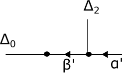
Figure 3: The graphical representation of a conformal block where a regular puncture and a rank $1$ puncture are realized inside a rank $1$ channel of momentum $\beta^{\prime}$.

This basis will also turn out to be useful as an intermediate step in the analysis of relations between the basis $|R^{(2)}(\beta)\rangle$ for regular vectors, and the basis $|I^{(2)}(\beta)\rangle$. We will indicate how vectors $|IR^{(1)}(\beta)\rangle$ can be constructed in a simple, careful collision limit from the usual $|R^{(2)}(\beta)\rangle$. Furthermore, the power series defining the vectors $|IR^{(1)}(\beta)\rangle$ is now adequate to reproduce the vectors $|I^{(2)}(\beta)\rangle$ in a careful collision limit $z_{2}\to 0$. A diagrammatical representation of this sequence of operations is given in Figure 4.

Figure 4: The sequence of collision limits which give the conformal blocks of rank $2$.

The study of the collision limits gives another way to argue that vectors $|IR^{(1)}(\beta)\rangle$ and $|I^{(2)}(\beta)\rangle$ with series expansions (3.5) and (3.11), respectively, really exist, as will be discussed from two points of view in Appendix D.

3.5 Further generalizations

In the case of regular conformal blocks, there are several other useful bases of solutions for the Ward identities with $n$ punctures. Indeed, the chiral vertex operator $\Psi^{\alpha}_{\alpha_{f},\alpha_{i}}(z)$ can be readily promoted to a map ${\mathcal{V}}_{\alpha_{i}}\to{\mathcal{V}}_{\alpha}\otimes{\mathcal{V}}_{\alpha_{f}}$, using Virasoro Ward identities in order to place descendants of the primary of dimension $\alpha$ at z. Then one can fuse the punctures in any order, forming a basis labeled by a rooted binary tree

$$|R_{n}\rangle=\Psi_{\alpha_{f},\beta_{1}}^{\beta_{2}}\left[\Psi_{\beta_{1},\beta_{3}}^{\beta_{4}}[\cdots],\Psi_{\beta_{2},\beta_{5}}^{\beta_{6}}[\cdots]\right]$$ (3.13)

In the case with irregular punctures, one can similarly promote $\Psi_{\beta^{(n)},\alpha^{(n)}}^{\alpha_{z}}(z)$ to a map ${\mathcal{V}}_{\alpha}\otimes{\mathcal{I}}_{n}\to{\mathcal{I}}^{\prime}_{n}$. Exchanging the role of $0$ and $z$, one can thus define a map $\Psi_{\beta^{(n)},\alpha}^{\alpha^{(n)}}$ which fuses a rank $n$ irregular vector at $z$ and a regular vector at the origin into a rank $n$ irregular module. Then starting from

$$\Psi_{\gamma^{(n)},\beta^{(n)}}^{\alpha_{w}}(w)\Psi_{\beta^{(n)},\alpha}^{\alpha^{(n)}}|\alpha\rangle$$ (3.14)

and colliding $w\to 0$ it may be possible to define a formal power series for $\Psi_{\beta^{(n)},\alpha^{\prime}}^{\alpha^{(n)}}(z)|I_{1}\rangle$ which fuses an irregular vector of rank $n$ and an irregular vector of rank $1$ into an irregular module of rank $n+1$. Iterating this procedure, one may arrive to the most general map $\Psi_{\beta^{(n+m)},\alpha^{(n)}}^{\alpha^{(m)}}$, fusing irregular punctures of rank $n$ and $m$ into an irregular module of rank $n+m$. These maps could be combined to produce very general bases of conformal blocks with irregular singularities, which explore more general boundary components of Teichmüller space for several irregular punctures. We leave a more detailed discussion of such possibilities to the future.

4 Free field construction

As an alternative approach to the construction of bases for spaces of irregular vectors we will now describe constructions based on the free field representation of the Virasoro algebra. This will give strong additional support for our previous claims about existence of irregular vectors with a certain structure of their expansions around the degeneration limit. It will furthermore give strong hints towards the existence of Stokes phenomena in such limits.

4.1 Primary fields

At first, we can review the free field construction of chiral vertex operators. We will mostly consider the case that $Q>2$ in the following, corresponding to central charge $c>25$. It turns out, however, that the results that we obtain for this regime have an analytic continuation w.r.t. the parameter $Q$ which allows one to cover the case $c>1$ as well. The basic building blocks of all constructions will be the following objects:
Normal ordered exponentials :

$${\mathsf{E}}^{\alpha}(z)\,\equiv\,\exp\Bigg{(}2\alpha\sum_{k<0}\frac{i}{k}a_{k}z^{-k}\Bigg{)}\,e^{2\alpha(q-\alpha_{p}\log z)}\,\exp\Bigg{(}2\alpha\sum_{k>0}\frac{i}{k}a_{k}z^{-k}\Bigg{)}\,.$$ (4.1)

Screening charges:

$${\mathsf{Q}}(z)\;\equiv\;\lim_{\epsilon\downarrow 0}\int_{{\mathcal{C}}_{z,\epsilon}}dw\;{\mathsf{E}}^{b}(w)\;,$$ (4.2)

with integration contour being the circle ${\mathcal{C}}_{z,\epsilon}=\{w\in{\mathbb{C}};|w|=e^{\epsilon}|z|\}$.

Out of these building blocks we may now construct an important class of chiral primary fields,

$${\mathsf{V}}_{s}^{\alpha}(z)\;=\;\big{(}{\mathsf{Q}}(z)\big{)}^{s}\,{\mathsf{E}}^{\alpha}(z)\;.$$ (4.3)

These objects are a priori only defined under suitable restrictions on the parameters $\alpha$, $s$ and $b$ which ensure that the short-distance singularities arising from the operator product expansions of the fields in (4.3) are all integrable. Similar objects can be defined for more general values of the parameters $\alpha$, $b$ and $s$ by analytic continuation [T04]. For explicit calculations it may also be useful to replace $({\mathsf{Q}}(z))^{s}$ in (4.3) by expressions of the form $\int_{\Gamma_{1}}dt_{1}\dots\int_{\Gamma_{s}}dt_{s}\,{\mathsf{E}}^{b}(t_{1})\cdots{\mathsf{E}}^{b}(t_{s}){\mathsf{E}}^{\alpha}(z)$ for a suitable collection of contours $\Gamma_{1},\dots,\Gamma_{n}$.

The covariant transformation law under conformal transformations,

$$[L_{k},{\mathsf{V}}_{s}^{\alpha}(z)]\,=\,z^{k}(z\partial_{z}+\Delta_{\alpha}(k+1)){\mathsf{V}}_{s}^{\alpha}(z)\,,$$ (4.4)

follows from the well-known facts that the fields $E^{\alpha}(z)\equiv{\mathsf{V}}_{0}^{\alpha}(z)$ satisfy this transformation law, and that the fields ${\mathsf{E}}^{b}(w)$ transform as total derivatives due to $\Delta_{b}=1$.

4.2 Irregular vectors

To begin with, let us introduce coherent states $|{\mathbf{c}};\alpha\rangle^{(n)}$ as before, defined by the properties

$$\begin{aligned} &a_{k}\,|\,{\mathbf{c}}\,;\alpha\,\rangle^{(n)}\,=\,-ic_{k}\,|c;\alpha\,\rangle^{(n)}\,,\\ &a_{k}\,|\,{\mathbf{c}}\,;\alpha\,\rangle^{(n)}\,=\,0\,,\end{aligned}\qquad\begin{aligned} &{\rm for}\;\;0<k\leq n\,,\\ &{\rm for}\;\;k>n\,.\end{aligned}$$ (4.5)

and thus satisfy the Ward identities for irregular vectors of degree $n$. The vectors $|{\mathbf{c}}\,;\alpha\rangle^{(n)}$ can be considered as coherent states created from the Fock vacuum $|\alpha\rangle$ as

$$|\,{\mathbf{c}}\,;\alpha\,\rangle^{(n)}\,=\,\exp\Bigg{(}\sum_{k=1}^{n}\frac{1}{n}c_{n}a_{-n}\Bigg{)}|\alpha\rangle\,.$$ (4.6)

More general irregular vectors may then be constructed by acting on the vectors $|{\mathbf{c}}\,;\alpha\rangle^{(n)}$ with powers of the operators ${\mathsf{Q}}_{\gamma}$

$${\mathsf{Q}}_{\gamma}\;\equiv\;\int_{\gamma}dw\;{\mathsf{E}}^{b}(w)\;,$$ (4.7)

where $\gamma$ is any contour that starts and ends at $w=0$ in sectors for which ${\rm Re}(c_{n}/w^{n})<0$. There are $n$ such sectors, explicitly given by

$${\mathcal{S}}_{k}^{(n)}:=\left\{\,w\in{\mathbb{C}}\,;\,-\frac{\pi}{2}+2\pi k<n\arg(w)-(\gamma_{n}-\pi)<-\frac{\pi}{2}+2\pi k\,\right\}\,,$$ (4.8)

for $k=0,\dots,n$. Vectors like

$$\left({\mathsf{Q}}_{\gamma_{1}}\right)^{s_{1}}\,\cdots\,\left({\mathsf{Q}}_{\gamma_{m}}\right)^{s_{m}}\,|\,{\mathbf{c}}\,;\alpha\,\rangle^{(n)}$$ (4.9)

will then be well-defined for collections of non-intersecting contours $\gamma_{1},\dots,\gamma_{m}$ of the type introduced above. Moreover, the operators ${\mathsf{Q}}_{\gamma}$ are easily seen to commute with the Virasoro generators. This implies that the vectors defined in (4.9) behave under conformal transformation in the same way as the vectors $|{\mathbf{c}}\,;\alpha\rangle^{(n)}$. One can consider a basis of $n$ non-intersecting contours $\gamma_{l}$ which start and end at $w=0$ in the sectors ${\mathcal{S}}_{k}^{(n)}$, and thereby generate families of irregular vectors which depend on $n$ additional positive-integer valued parameters $s_{1},\dots,s_{n}$.

Notice that there are several inequivalent choices of set of $n$ contours $\gamma_{l}$, which give distinct bases of irregular vectors. For example, one could consider the $n$ “shortest” contours, joining consecutive sectors. Alternatively, one could use nested sets of longer contours. Some examples are shown in Figure 5.

Figure 5: Examples of screening paths. From left to right, the unique rank $1$ example, a rank $2$ example with two short paths, another rank $2$ example

We can now consider collision and degeneration limits in the free field setup, in order to match the free-field bases of irregular vectors with the formal power series built from expansion over descendants of irregular vectors.

4.3 Degeneration limits

4.3.1 Saddle point analysis

In a degeneration limit the singularity of $\partial\phi(y)$ goes from $n+1$ to $n$. Correspondingly, there must be a zero $y_{{\mathbf{c}}}$ of $\partial\phi(y_{{\mathbf{c}}})$ which moves to the origin. The approximate position of the zero is $-c_{n}/c_{n-1}$ and it is easy to see that the value of $\phi(y_{{\mathbf{c}}})$ diverges as $c_{n}\to 0$. This has an interesting implication: the zero $y_{{\mathbf{c}}}$ of $\partial\phi(y)$ is a saddle for the screening charge contour integral, and the saddle point approximation is increasingly good in the degeneration limit for an integration contour corresponding to the steepest descent contour of $y_{{\mathbf{c}}}$.

This means that any screening contours which can be deformed to the steepest descent contour will collapse in the degeneration limit, and their contribution can be computed in the saddle point approximation. The position of the saddle point and the value of $\partial\phi(y)$ on the saddle are not affected much by the presence of other screening charges. The value on the saddle is controlled by the value $\phi_{\mathrm{sing}}(y_{{\mathbf{c}}})$ of

$$\phi_{\mathrm{sing}}(y)=\frac{c_{n}}{ny^{n}}+\frac{c_{n-1}}{(n-1)y^{n-1}}+\cdots+\frac{c_{1}}{y}$$ (4.10)

plus logarithmic terms which are affected by the other screening charges.

Let us apply these observations to the study of the behavior of an irregular vector of rank $n$ of the form

$$\left({\mathsf{Q}}_{\gamma_{1}}\right)^{s_{1}}\,\cdots\,\left({\mathsf{Q}}_{\gamma_{n}}\right)^{s_{n}}\,|\,{\mathbf{c}}\,;\alpha_{n}\rangle^{(n)}$$

in a degeneration limit where $c_{n}\to 0$. Let us assume that $\gamma_{n}$ can be deformed to the steepest descent contour for the saddle point which is collapsing to the origin, while the $\gamma_{1},\dots,\gamma_{n-1}$ are chosen so that they do not receive contributions from that saddle point, i.e. do not intersect the path of steepest ascent from that saddle. When $c_{n}\to 0$ we will then get an irregular vector of order $n-1$ proportional to

$$\left({\mathsf{Q}}_{\gamma_{1}^{\prime}}\right)^{s_{1}}\,\cdots\,\big{(}{\mathsf{Q}}_{\gamma_{n-1}^{\prime}}\big{)}^{s_{n-1}}\,|\,{\mathbf{c}}^{(n-1)}\,;\alpha_{n-1}\rangle^{(n-1)}\,,$$

multiplied with a prefactor which contains

$$e^{2bs_{n}\phi_{\rm sing}(y_{{\mathbf{c}}})}\,=\,e^{-2(\alpha_{n}-\alpha_{n-1})\phi_{\rm sing}(y_{{\mathbf{c}}})}\,.$$ (4.11)

The contours $\gamma_{1}^{\prime},\dots,\gamma_{n-1}^{\prime}$ are obtained from $\gamma_{1},\dots,\gamma_{n-1}$ by deforming these contours such that they start and end in the sectors ${\mathcal{S}}_{k}^{(n-1)}$. The logarithmic terms give important powers of $c_{n}$, which are harder to compute from the free field analysis.

It may be instructive to observe that the free field construction gives a rather concrete realization of the intertwining operators $\Psi^{n-1,n}_{\beta^{(n-1)},\beta^{(n)}}({\mathbf{c}})$ introduced in Section 3. Indeed, by expanding

$$|\,{\mathbf{c}}\,;\alpha_{n}\rangle^{(n)}\,=\,\sum_{m=0}^{\infty}\frac{c_{n}^{m}}{m!}(a_{-n})^{m}\,|\,{\mathbf{c}}^{(n-1)}\,;\alpha_{n-1}\rangle^{(n-1)}\,,$$ (4.12)

combined with an application of the saddle-point method as outlined above one will get a representation for $\left({\mathsf{Q}}_{\gamma_{n}}\right)^{s_{n}}|{\mathbf{c}}\,;\alpha_{n}\rangle^{(n)}$ as a formal series in powers of $c_{n}$ of the form

$$\left({\mathsf{Q}}_{\gamma_{n}}\right)^{s_{n}}\,|\,{\mathbf{c}}\,;\alpha_{n}\rangle^{(n)}\,=\,e^{-2(\alpha_{n}-\alpha_{n-1})\phi_{\rm sing}(y_{{\mathbf{c}}})}\prod_{k=1}^{n}c_{k}^{\nu_{k}}\sum_{m=0}^{\infty}c_{n}^{m}\,|\,{\mathbf{c}}^{(n-1)}\,;\alpha_{n-1};m\,\rangle^{(n-1)},$$ (4.13)

where the $|{\mathbf{c}}^{(n-1)}\,;\alpha_{n-1};m\,\rangle^{(n-1)}$ are generalized descendants of $|{\mathbf{c}}^{(n-1)}\,;\alpha_{n-1}\,\rangle^{(n-1)}$. It follows that the formal expansion in powers of $c_{n}$ of $\left({\mathsf{Q}}_{\gamma_{n}}\right)^{s_{n}}|{\mathbf{c}}\,;\alpha_{n}\rangle^{(n)}$ represents the intertwiner $\Psi^{n-1,n}_{\beta^{(n-1)},\beta^{(n)}}({\mathbf{c}})$ within the free field representation.

4.3.2 Stokes phenomena

In a degeneration limit where $c_{n}/c_{n-1}\to 0$, there will be a unique steepest descent contour $\gamma_{n}$ for the saddle point which tends to the origin in this limit. The remaining contours can always be assumed to have zero intersection with the contour of steepest ascent. Using such contours in the construction above will define irregular vectors which have an asymptotic behavior for $c_{n}/c_{n-1}\to 0$ that is well-approximated by the formal series (4.13) only in a certain sector of the complex plane parameterized by $c_{n}/c_{n-1}$. Indeed, assuming for example that for a given initial value of the parameters $c$ the steepest descent contour $\gamma_{n}$ ends in the sector ${\mathcal{S}}_{n}^{(n)}$, a variation of the phase of $c_{n-1}$ may move the phase of the saddle point $-c_{n}/c_{n-1}$ too far away from the sector ${\mathcal{S}}_{n}^{(n)}$ for having a steepest descent contour that would still end in ${\mathcal{S}}_{n}^{(n)}$. We conclude that there are Stokes phenomena in the asymptotic behavior of irregular vectors in the degeneration limit.

Figure 6: A choice of screening paths with good degeneration limit. The open circle denotes the saddle point, the dashed path is the steepest ascent path.

We may observe an analogy with the classification of different natural bases for regular conformal blocks: Different natural bases are labelled by the boundary components of the Teichmüller space of the Riemann surface one is working on. The elements of a basis associated to a given boundary component are characterized by having a simple form of the expansion in powers of the gluing parameters in the given boundary component only. They may be analytically continued to other boundary components, but will have a much more complicated behavior there. There exist, however, linear transformations between the bases associated to different boundary components that can be decomposed into the so-called fusion-, braiding- and modular transformation moves.

Considering conformal blocks in cases with irregular singularities, the considerations above strongly suggest that the data classifying boundary components of the Teichmüller spaces may include the choices of Stokes sectors. A given basis for the space of conformal blocks is characterized by having a simple asymptotic expansion only in one particular Stokes sector. The analytic continuation of the elements of a given basis associated to one Stokes sector into another sector will be shown in the second part of this series to be representable as linear combinations of the elements of the basis associated to the other sector. The chiral bootstrap is in the irregular case therefore characterized by an enlarged set of data containing analogs of the Stokes matrices in addition to the fusion-, braiding- and modular transformation matrices (or integral kernels). The second part in this series will in particular contain explicit calculations of these data.

Let us finally stress one important observation: Vectors like $\left({\mathsf{Q}}_{\gamma_{n}}\right)^{s_{n}}|c;\alpha_{n}\rangle^{(n)}$ which can be expanded as in (4.13) are perfectly well-defined objects. Identifying the expansion on the right hand side of (4.13) with the formal expansion of the intertwiner $\Psi^{k-1,k}_{\beta^{(k-1)},\beta^{(k)}}(c_{k})$ suggests that the conformal blocks constructed using this intertwiner do not only exist in the sense of formal series, but that there exist actual functions for which the algebraic constructions discussed above give the asymptotic series expansions in suitable Stokes sectors.

4.4 Collision limits

The free field representation is in many respects particularly well-suited for discussing the production of irregular vectors in collision limits. In order to illustrate some important qualitative features we will restrict attention to the case $n=2$, leaving the discussion of more general cases to the future. Let us start from

$${\mathsf{V}}^{\alpha_{1}}_{s_{1}}(z_{1}){\mathsf{V}}^{\alpha_{2}}_{s_{2}}(z_{2})|\,\alpha_{3}\,\rangle\,.$$ (4.14)

The normal ordered exponential fields satisfy exchange relations of the form

$${\mathsf{E}}^{\alpha_{1}}(z_{1}){\mathsf{E}}^{\alpha_{2}}(z_{2})\,=\,e^{-2\pi i\alpha_{1}\alpha_{2}}{\mathsf{E}}^{\alpha_{2}}(z_{2}){\mathsf{E}}^{\alpha_{1}}(z_{1})\,,$$ (4.15)

valid for $|z_{1}|=|z_{2}|$, $\arg(z_{1})>\arg(z_{2})$. Introduce the partial screening charges

$${\mathsf{Q}}_{I}:=\int_{z_{2}}^{z_{1}}dw\;{\mathsf{Q}}^{b}(w)\,,\qquad{\mathsf{Q}}_{I^{\prime}}:=\int_{z_{1}}^{\hat{z}_{2}}dw\;{\mathsf{Q}}^{b}(w)\,,$$ (4.16)

where $\hat{z}_{2}:=e^{2\pi i}z_{2}$. The exchange relation (4.15) allows us to move the normal ordered exponentials in the definition of (4.14) to the right of the screening charges. Assuming $\arg(z_{1})>\arg(z_{2})$ we thereby find

$$\big{[}{\mathsf{Q}}(z_{1})\big{]}^{s_{1}}{\mathsf{E}}^{\alpha_{1}}(z_{1})\, \big{[}{\mathsf{Q}}_{I}+{\mathsf{Q}}_{I^{\prime}}\big{]}^{s_{2}}{\mathsf{E}}^{\alpha_{1}}(z_{2})\,=$$ (4.17)

$$=\, \big{[}{\mathsf{Q}}(z_{1})\big{]}^{s_{1}}\,\big{[}e^{-2\pi ib\alpha_{1}}{\mathsf{Q}}_{I}+e^{2\pi ib\alpha_{1}}{\mathsf{Q}}_{I^{\prime}}\big{]}^{s_{2}}\,{\mathsf{E}}^{\alpha_{1}}(z_{1}){\mathsf{E}}^{\alpha_{2}}(z_{2})\,.$$

In this form it becomes straightforward to take the collision limits producing irregular vectors of degree $2$. The collision limits of ${\mathsf{E}}^{\alpha_{1}}(z_{1}){\mathsf{E}}^{\alpha_{2}}(z_{2})|\alpha_{3}\rangle$ produce vectors $|c;\alpha^{\prime\prime}\rangle^{(2)}$ with $\alpha^{\prime\prime}=\alpha_{1}+\alpha_{2}+\alpha_{3}$. It is furthermore easy to show that the partial screening charge ${\mathsf{Q}}_{I}$ becomes the operator ${\mathsf{Q}}_{\gamma}$ with contour $\gamma$ which connects sector ${\mathcal{S}}_{2}$ with ${\mathcal{S}}_{1}$, while ${\mathsf{Q}}_{I^{\prime}}$ turns into the operator ${\mathsf{Q}}_{\gamma^{\prime}}$ associated to the contour $\gamma^{\prime}$ which connects ${\mathcal{S}}_{1}$ with $e^{2\pi i}{\mathcal{S}}_{2}$. The operator ${\mathsf{Q}}(z_{1})$ becomes an operator ${\mathsf{Q}}_{\xi}$ associated to a contour $\xi$ which starts in ${\mathcal{S}}_{1}$, encircles $w=0$ and ends in $e^{2\pi i}{\mathcal{S}}_{1}$.

What is interesting to observe is the fact that there are two different ways to take the limit of (4.17) which yield either

$$\big{[}{\mathsf{Q}}_{\xi}\big{]}^{s_{1}}\big{[}{\mathsf{Q}}_{\gamma}\big{]}^{s_{2}}|\,{\mathbf{c}};\alpha^{\prime\prime}\,\rangle^{(2)}\,,\qquad{\rm or}\qquad\big{[}{\mathsf{Q}}_{\xi}\big{]}^{s_{1}}\big{[}{\mathsf{Q}}_{\gamma^{\prime}}\big{]}^{s_{2}}|\,{\mathbf{c}};\alpha^{\prime\prime}\,\rangle^{(2)}\,,$$ (4.18)

as a result, depending on whether ${\rm Im}(\alpha_{1})$ tends to $\pm\infty$ in the limit.

One of the main points to be observed here is the fact that after multiplying with some simple numerical factors we get vectors that stay finite in the collision limits.

5 Conformal blocks from solutions of null vector equations

Degenerate fields in Liouville theory satisfy differential equations. We will use these differential equations in order to get an alternative approach to the definition of bases in the space of conformal blocks, the calculation of their series expansions, and for the study of the collision limits producing irregular singularities.

This is necessarily somewhat tricky, as generic conformal blocks do not satisfy a closed system of partial differential equations. The idea may be informally described as follows: Inserting additional degenerate fields into the conformal block gives modified conformal blocks that satisfy the differential equations following from null vector decoupling. These differential equations can be used to obtain power series expansions for the modified conformal blocks. The original conformal block can be recovered in a certain limit where the additional degenerate fields fuse with some of the primary fields inserted into the modified conformal blocks. In order to calculate this limit it suffices to know the braiding transformations involving degenerate fields, which is explicitly known. We will show how this idea can be used to calculate series expansions for conformal blocks involving both regular and irregular vertex operators.

5.1 Degenerate chiral vertex operators

Let us consider the special chiral vertex operators

$$V_{\pm}(y)\,\equiv\,\Psi^{-b/2}_{\beta^{\prime},\beta}(y)\,.$$ (5.1)

It is well-known that these vertex operators satisfies the operator differential equation

$$\frac{1}{b^{2}}\frac{\partial^{2}}{\partial y^{2}}\,V_{\pm}(y)\,+:T(y)V_{\pm}(y):\,=\,0\,,$$ (5.2)

with normal ordering $:T(y)V_{\pm}(y):$ defined as

$$:T(y)V_{\pm}(y):\,\equiv\sum_{k<-1}y^{-k-2}L_{k}V_{\pm}(y)+\sum_{k\geq-1}y^{-k-2}V_{\pm}(y)L_{k}\,.$$ (5.3)

The operator differential equation (5.2) is equivalent to the decoupling of null vectors in the Verma module of descendants of $V_{\pm}(y)$. We will therefore call the equations following from (5.2) null vector equations. Note in particular that conformal blocks containing insertions of $V_{\pm}(y)$ like

$${\mathcal{F}}(y)\equiv{\mathcal{F}}(y;z_{1},z_{2}):=\big{\langle}\,\alpha_{0}\,|\,\Psi^{\alpha_{1}}_{\alpha_{0},\beta^{\prime}}(z_{1})\,V_{+}(y)\,\Psi^{\alpha_{2}}_{\beta,\alpha_{3}}(z_{2})\,|\,\alpha_{3}\,\big{\rangle}\,,$$ (5.4)

will satisfy a partial differential equation of second order in $\frac{\partial}{\partial y}$ which is obtained by moving the Virasoro generators in $:T(y)V_{\pm}(y):$ to the left or right until they hit the highest weight vectors. The resulting differential equation is of the generic form

$$\left(\frac{1}{b^{2}}\frac{\partial^{2}}{\partial y^{2}}+{\mathcal{T}}(y)\right){\mathcal{F}}(y;z_{1},z_{2})\,=\,0\,,$$ (5.5)

where ${\mathcal{T}}(y)$ is a first order differential operator which for the case (5.4) above is explicitly given as

$${\mathcal{T}}(y):= \frac{\Delta_{1}}{(y-z_{1})^{2}}+\frac{\Delta_{2}}{(y-z_{2})^{2}}+\frac{\Delta_{3}}{y^{2}}+\frac{1}{y-z_{1}}\frac{z_{1}}{y}\frac{\partial}{\partial z_{1}}+\frac{1}{y-z_{2}}\frac{z_{2}}{y}\frac{\partial}{\partial z_{2}}-\frac{1}{y}\frac{\partial}{\partial y}\,.$$

We are using the notations $\Delta_{\alpha_{r}}=\alpha_{r}(Q-\alpha_{r})$, $r=0,1,2,3$, $\delta_{b}=-\frac{1}{2}-\frac{3}{4}b^{2}$.

5.1.1 Fusion rules

The null decoupling condition can only hold if one restricts the Liouville momentum $\beta$ to jump across the degenerate field as $\beta^{\prime}=\beta\pm b/2$. Indeed, if we apply this relation to the leading term in the expansion of $V_{\pm}(z)|\Delta_{\beta}\rangle$ and denote $\delta=\Delta_{\beta^{\prime}}-\Delta_{\beta}-\Delta_{-b/2}$, we get the constraint $\delta(\delta-1-b^{2})+b^{2}\Delta_{\beta}=0$. This is solved by $\delta=b\beta$ or $\delta=b(Q-\beta)$, which means $\beta^{\prime}=\beta-b/2$ or $\beta^{\prime}=\beta+b/2$, respectively. It is known that this condition is also sufficient for $V(z)$ to satisfy the null vector equation. We will also denote the solutions with $\beta^{\prime}=\beta\mp b/2$ as

$$V_{\pm}(y)\,\equiv\,V_{\beta;\pm}(y)\,\equiv\,\Psi^{-b/2}_{\beta\mp b/2,\beta}(y)\,.$$ (5.6)

Notice that $\delta$ controls the monodromy of $V(y)$ around the origin. This fact is of crucial importance, as it represents a link between the characterization of bases for the spaces of conformal blocks in terms of the series expansions for solutions of the null vector equations on the one hand, to the characterization in terms of Verlinde line operators [AGGTV, DGOT] on the other hand. The latter is closely connected to the characterization of bases for the spaces of conformal blocks by means of the geodesic length operators in quantum Teichmüller theory.

We can easily repeat the analysis to find the constraints appropriate for the vertex operator $V^{(1)}(y)$ which represents the insertion of a degenerate field near a rank $1$ irregular vector as a sum over generalized descendants of the rank $1$ irregular vector. Thus in order for $V^{(1)}(y)$ to satisfy the null vector decoupling, it must shift the Liouville momentum of the irregular puncture by $\pm b/2$. We can thus define

$$V^{(1)}_{\pm}(y)\,\equiv\,V_{\beta^{\prime};\pm}^{(1)}(y):=\Psi^{-b/2(1)}_{\beta^{\prime}\mp b/2,\beta^{\prime}}(y)\,.$$ (5.7)

This reasoning readily extends to the vertex operators $V^{(n)}_{\pm}(y)$.

5.1.2 Monodromy and formal monodromy

Notice an important fact. Our expansion (3.11) for $V^{(1)}_{\pm}(z)$ has a prefactor $y^{\nu}c_{1}^{\nu_{1}}\,e^{(\beta^{\prime}-\alpha^{\prime})\frac{2c_{1}}{y}}$ where

$$\nu=-2\Delta_{-b/2}-2(\beta^{\prime}-Q)(\beta^{\prime}-\alpha^{\prime})=1+3/2b^{2}\mp b(\beta^{\prime}-Q)$$ (5.8)

which means either $\nu=b\alpha^{\prime}$ or $\nu=b(2Q-\alpha^{\prime})$. The parameter $\nu$ controls the formal monodromy of the asymptotic expansion. This is a rather intuitive result. If the irregular puncture arises from the collision of two regular punctures, of Liouville momenta which add to $\alpha^{\prime}$, it appears that the formal monodromy around the irregular puncture is simply the sum of the monodromy eigenvalues around each individual puncture.

The formal monodromy is a very important piece of information. We expect it to provide a link between the bases for the irregular conformal blocks constructed in this paper and the irregular generalization of the quantum Teichmüller theory.

Furthermore, this confirms the expectation that the solutions built from $V^{(1)}_{\pm}(y)$ may be well-defined beyond the formal power series definition, but depend on a choice of Stokes sector where the expansion would be valid. In the case of the degenerate insertion, the exponential prefactor $\exp\pm\frac{bc_{1}}{y}$ suggests that there are two possible choices of Stokes sector: sectors including either of the two half-lines $\frac{y}{c_{1}}\in\pm i{\mathbb{R}}^{+}$.

Finally, we can extend the formal monodromy statement to any rank $k$. We expect that for an irregular puncture of rank $k$ and momentum $\alpha_{k}$ at the origin, the degenerate insertion will shift the Liouville momentum by $\pm b/2$, and will have formal monodromy $\nu=b\alpha_{k}$ or $\nu=b((k+1)Q-\alpha_{k})$. We can test this at the leading order of the $y$ expansion for $V^{(k)}_{\pm}(y)|I_{k}\rangle$. The null decoupling constraint takes the form

$$\left(\partial_{y}^{2}-b^{2}y^{-1}\partial_{y}\right)+b^{2}T_{\gg}(y)$$ (5.9)

where with $T_{\gg}(y)$ we denote the singular part of $T(y)$ near the irregular vector, excluding the $L_{-1}$ piece. This constraint can be patiently applied to the ansatz

$$y^{\nu}\exp\pm\sum_{n=1}^{k}\frac{c_{n}}{ny^{n}}$$ (5.10)

to verify that this ansatz can be the starting point of a systematic asymptotic expansion of the solution. We refer the reader to section C.2 for an example of such systematic expansion, at rank $2$.

5.2 Construction of bases with the help of null vector equations - the regular case

We now want to explain in some more detail how to use the null vector equations in order to construct certain bases for the space of conformal blocks. As indicated above, the basic idea is to first consider conformal blocks which contain degenerate fields $V_{\pm}(y)$, exploit the information given by the differential equations that such conformal blocks satisfy, and finally remove the degenerate fields by taking some limit which produces conformal blocks without degenerate fields. We’ll here give an outline of this procedure, leaving several details to Appendix C.

Let us explain the basic idea a bit more precisely in the case $n=0$. The object of our interest is the expansion of the conformal block

$$F(z_{1},z_{2}):=\,\big{\langle}\,\alpha\,|\,\Psi^{\alpha_{1}}_{\alpha,\beta}(z_{1})\Psi^{\alpha_{2}}_{\beta,\alpha_{3}}(z_{2})\,|\,\alpha_{3}\,\big{\rangle}$$ (5.11)

in powers of $z_{2}$. The scaling properties of this conformal block imply the general form

$$F(z_{1},z_{2})\,=\,z_{1}^{\Delta_{\alpha}-\Delta_{\alpha_{1}}-\Delta_{\alpha_{2}}-\Delta_{\alpha_{3}}}\sum_{k=0}^{\infty}\left(\frac{z_{2}}{z_{1}}\right)^{\chi+k}F_{k}\,.$$ (5.12)

As a technical tool for its study we shall modify the conformal blocks by additional insertions of the special chiral vertex operators $V_{\pm}(y)$.

The differential equations satisfied by ${\mathcal{F}}(y;z_{1},z_{2})$ will turn out to have a unique solution in the form of a double power series in $z_{2}/y$ and $y/z_{1}$ such that

$${\mathcal{F}}(y;z_{2},z_{1})\,=\,\sum_{k=0}^{\infty}\left(\frac{z_{2}}{y}\right)^{\chi+k}\!\!{\mathcal{F}}_{k}(y;z_{1})\,,\quad{\mathcal{F}}_{k}(y;z_{1})\,=\,z_{1}^{\kappa}\sum_{l=0}^{\infty}\left(\frac{y}{z_{1}}\right)^{\eta+l}\!\!{\mathcal{F}}_{k,l}\,,$$ (5.13)

where

$$\kappa\,=\,\Delta_{0}-\Delta_{1}-\Delta_{2}-\Delta_{3}-\delta_{b}\,,\qquad\chi\,=\,\Delta_{\beta}-\Delta_{\alpha_{2}}-\Delta_{\alpha_{3}}\,,\qquad\eta\,=\,b\beta\,.$$ (5.14)

This form of the series as specified in (5.13) is necessary for the solution to be identified with the conformal block ${\mathcal{F}}(y;z_{1},z_{2})$. It follows from the representation theoretic construction of the conformal blocks by summing over states from fixed intermediate representations.

To avoid confusions, let us note that it is not at all straightforward to find series expansions in $z_{1}/y$ that could be identified with the conformal blocks ${\mathcal{E}}(y;z_{2},z_{1}):=\big{\langle}\alpha_{0}|V_{\pm}(y)\Psi^{\alpha_{1}}_{\alpha_{0}\pm b/2,\beta}(z_{1})\Psi^{\alpha_{2}}_{\beta,\alpha_{3}}(z_{2})\,|\,\alpha_{3}\,\big{\rangle}$. The differential equation does not give any constraints on the leading coefficients ${\mathcal{E}}_{k,0}$ of an expansion like

$${\mathcal{E}}(y;z_{2},z_{1})\,=\,\sum_{k=0}^{\infty}\left(\frac{z_{2}}{y}\right)^{\chi+k}\!\!{\mathcal{E}}_{k}(y;z_{1})\,,\quad{\mathcal{E}}_{k}(y;z_{1})\,=\,z_{1}^{\kappa}\sum_{l=0}^{\infty}\left(\frac{z_{1}}{y}\right)^{\eta^{\prime}+l}\!\!{\mathcal{E}}_{k,l}\,.$$ (5.15)

It is therefore necessary for us to start from an expansion of the form (5.13), and continue analytically to $y\to\infty$ afterwards to recover the conformal block $F(z_{1},z_{2})$ we are after. As a tool for carrying out this analytic continuation we may use the exchange relation

$$\Psi^{\alpha_{1}}_{\alpha_{0},\beta-b/2}(z_{1})\,V_{\beta;+}(y)\,=$$ (5.16)

$$\quad\,=\,B_{+}(s)\,V_{\alpha_{0}+b/2;+}(y)\Psi^{\alpha_{1}}_{\alpha_{0}+b/2,\beta}(y)+B_{-}(s)\,V_{\alpha_{0}-b/2;-}(y)\Psi^{\alpha_{1}}_{\alpha_{0}-b/2,\beta}(y)\,,$$

valid for $|z_{1}|=|y|$ furthermore allows us perform the analytic continuation to $|y|>|z_{1}|$. The coefficients $B_{\pm}(s)$ in (5.16) depend on $s:=\operatorname{sgn}(\arg(z_{1}/y))$, as usual. One may then study the limit $y\to\infty$ using the OPE

$$\big{\langle}\,\alpha_{0}\,|\,V_{\alpha_{0}+\epsilon b/2;\epsilon}(y)\,=\,\big{\langle}\,\alpha_{0}+\epsilon b/2\,|\;y^{\frac{1}{2}(2b^{2}+1)+\epsilon b(\alpha_{0}-Q/2)}\,\big{(}C_{\epsilon}+{\mathcal{O}}(y^{-1})\big{)}\,.$$ (5.17)

Assuming that $\Re(2\alpha_{0}-Q)>0$, the term with $\epsilon=1$ in (5.17) dominates for $y\to\infty$. Let us assume that $s=1$ and set $B_{+}\equiv B_{+}(1)$. Assuming furthermore that $\alpha=\alpha_{0}+b/2$, we may then calculate the sought-for coefficients $F_{k}$ as

$$F_{k}\,=\,\frac{1}{C_{+}B_{+}}\lim_{y/z_{1}\to\infty}y^{-b(\alpha_{0}+b/2)}z_{1}^{k-\kappa}{\mathcal{F}}_{k}(y;z_{1})\,.$$ (5.18)

We want to show that (5.18) leads to a purely algebraic procedure for the calculation of the expansion coefficients $F_{k}$. To this aim let us note that the representation theoretic definition of ${\mathcal{F}}(y;z_{1},z_{2})$ via (5.4) yields power series in $y/z_{1}$, $z_{2}/z_{1}$ convergent for $|z_{1}|>|y|>|z_{2}|$. The expansion in powers of $z_{2}$ can be obtained from (3.4). We thereby get an expansion for ${\mathcal{F}}(y;z_{1},z_{2})$ of the form (5.13). The coefficient functions ${\mathcal{F}}_{k}(y;z_{1})$ are proportional to the conformal blocks

$${\mathcal{F}}_{k}(y;z_{1})\,=\,y^{k}\,\langle\,\alpha_{0}\,|\,\Psi_{\alpha_{0},\beta-b/2}^{\alpha_{1}}(z_{1})\,V_{+}(y)\,|\,\beta,v_{k}\,\rangle\,,$$ (5.19)

where $|\,\beta,v_{k}\,\rangle$ is the descendant $\sum_{{I};|{I}|=k}C_{{I}}{{\mathbb{L}}}_{-{I}}|\,\beta\,\rangle$. By moving ${{\mathbb{L}}}_{-{I}}$ to the left in (5.19) above one may rewrite ${\mathcal{F}}_{k}(y;z_{1})$ in the form

$${\mathcal{F}}_{k}(y;z_{1}):=\,y^{k}{\mathcal{D}}_{k}(y,z_{1}){\mathcal{F}}_{0}(y;z_{1})\,,$$ (5.20)

where the differential operator ${\mathcal{D}}_{k}(y,z_{1}):=\sum_{{I};|{I}|=k}C_{{I}}{\mathbf{{\mathcal{L}}}}_{-{I}}(y,z_{1})$ creating ${\mathcal{G}}_{k}$ from ${\mathcal{G}}_{0}$ is obtained from $\sum_{{I};|{I}|=k}C_{{I}}{{\mathbb{L}}}_{-{I}}$ by replacing

$$L_{-k}\to-y^{-k}(y\partial_{y}+\Delta_{-b/2}(1-k))-z_{1}^{-k}(z_{1}\partial_{z_{1}}+\Delta_{1}(1-k))$$

from the left to the right. The differential operator ${\mathcal{D}}_{k}(y,z_{1})$ is of the form

$${\mathcal{D}}_{k}(y,z_{1})\,=\,\sum_{l=0}^{k}\left(\frac{z_{1}}{y}\right)^{l}\,\sum_{m=0}^{k}{\mathcal{D}}_{k;l,m}\left(y\frac{\partial}{\partial y}\right)^{m}\,,$$ (5.21)

as follows easily from its scaling behavior. The relation (5.20) will allow us to calculate the asymptotics ${\mathcal{F}}(y;z_{1},z_{2})$ in terms of the asymptotics of the lowest order term ${\mathcal{F}}_{0}(y;z_{1})$ as soon as we have determined the differential operator ${\mathcal{D}}_{k}$. Having constructed the full power series expansion (5.13) of ${\mathcal{F}}(y;z_{1},z_{2})$ one can view the relation (5.20) as a linear equation for the differential operator ${\mathcal{D}}_{k}(y,z_{1})$. It is equivalent to the linear system

$$\sum_{m=0}^{k}\,\sum_{\begin{subarray}{c}l^{\prime},l^{\prime\prime}=0\\ l^{\prime}+l^{\prime\prime}=l\end{subarray}}^{k}\,{\mathcal{D}}_{k;l^{\prime},m}\,(\eta+l^{\prime\prime})^{m}{\mathcal{F}}_{0,l^{\prime\prime}}\,=\,{\mathcal{F}}_{k,l}\,,$$ (5.22)

of equations for the coefficients ${\mathcal{D}}_{k;l,m}$ of ${\mathcal{D}}_{k}(y,z_{1})$. This is an infinite system of equations for a finite number of unknowns, so uniqueness of the solutions seems clear, while existence may not be obvious. The existence of solutions is here assured by the representation theoretic construction of the conformal blocks, as discussed in the above.

Inserting the relation (5.20) between ${\mathcal{F}}_{k}(y;z_{1})$ and ${\mathcal{F}}_{0}(y;z_{1})$ into (5.18) gives us the relation

$$F_{k}\,=\,y^{-b\alpha}\cdot{\mathcal{D}}_{k}(y;0)\cdot y^{b\alpha}=\sum_{m=0}^{k}{\mathcal{D}}_{k;0,m}\left(b\alpha\right)^{m}\,,\qquad\alpha=\alpha_{0}+b/2\,.$$ (5.23)

As the coefficients ${\mathcal{D}}_{k;l,m}$ can be calculated from the expansion coefficients ${\mathcal{F}}_{k,l}$ by solving (5.22), we thereby get a procedure to calculate the coefficients $F_{k}$ from the differential equation satisfied by the modified conformal blocks ${\mathcal{F}}(y;z_{1},z_{2})$.

5.3 The case of an irregular singularity or rank 2

We now want to consider the insertion of a degenerate vertex operator in the conformal block with a regular singularity at infinity, and a rank $2$ irregular singularity at the origin. The main idea is to use the degenerate field as a probe of the internal structure of the irregular singularity.

In order to make this idea more precise we will show that there exists a unique solution to the null vector decoupling equations that can be identified with the conformal blocks denoted as

$${\mathcal{F}}^{(2)}(y;c_{1},c_{2}):=\langle\,\alpha_{0}\,|\,\Psi^{r,1}_{\alpha_{0},\beta^{\prime}-b/2}(c_{1})V^{(1)}_{+}(y)\,\Psi^{1,2}_{\beta^{\prime},\alpha^{\prime\prime}}({\mathbf{c}})\,|\,I_{2}(\alpha^{\prime\prime})\,\rangle\,,$$ (5.24)

using the notations of Section 3. This should a priori not be confused with

$${\mathcal{E}}^{(2)}_{\pm}(y;c_{1},c_{2}):=\langle\,\alpha_{0}\,|\,V_{\pm}(y)\,\Psi^{r,1}_{\alpha_{0}\pm b/2,\beta^{\prime}}(c_{1})\Psi^{1,2}_{\beta^{\prime},\alpha^{\prime\prime}}({\mathbf{c}})\,|\,I_{2}(\alpha^{\prime\prime})\,\rangle\,.$$ (5.25)

The conformal blocks defined in (5.24) and (5.25) turn out to be closely related, however. ${\mathcal{F}}^{(2)}(y;c_{1},c_{2})$, initially being characterized near $y\to 0$ by an asymptotic double series in powers of $y/c_{1}$ and $c_{2}/yc_{1}$, can be analytically continued into the region where $y\to\infty$. As we will show later in this subsection, one may represent the result of this analytic continuation as a linear combination of the two conformal blocks ${\mathcal{E}}^{(2)}_{\pm}(y;c_{1},c_{2})$ defined in (5.25).

To begin with, let us use the expansion (3.5) to represent the conformal blocks ${\mathcal{E}}^{(2)}_{\pm}(y;c_{1},c_{2})$ as series in powers of $c_{2}$. The resulting expansion takes the form

$${\mathcal{E}}^{(2)}_{\pm}(y;c_{1},c_{2})\,=\,c_{2}^{\nu_{2}}c_{1}^{\nu_{1}}e^{(\alpha^{\prime\prime}-\beta^{\prime})\frac{c_{1}^{2}}{c_{2}}}\,\sum_{k=0}^{\infty}c_{2}^{k}\,{\mathcal{E}}^{(2)}_{k;\pm}(y;c_{1})$$ (5.26)

$${\rm where}\quad{\mathcal{E}}^{(2)}_{k;\pm}(y;c_{1}):=\langle\,\alpha_{0}\,|\,V_{\pm}(y)\,|\,I^{(1)}_{2k}(c_{1},\beta^{\prime})\,\rangle\,.$$ (5.27)

Assuming that the vectors $|\,I^{(1)}_{2k}(c_{1},\beta^{\prime})\,\rangle$ can be represented as generalized descendants of $|\,I^{(1)}(c_{1},\beta^{\prime})\,\rangle$, as we had proposed in Section 3, we may move the Virasoro generators in $|\,I^{(1)}_{2k}(c_{1},\beta^{\prime})\,\rangle$ to the left and get recursive relations of the form

$${\mathcal{E}}^{(2)}_{k;\pm}(y;c_{1})\,=\,{\mathcal{D}}_{k}(y,c_{1})\,{\mathcal{E}}^{(2)}_{0;\pm}(y;c_{1})\,.$$ (5.28)

Below we will show that ${\mathcal{E}}^{(2)}_{0;\pm}(y;c_{1})$ can be expressed in terms of the confluent hypergeometric functions. Taking into account (5.28) allows us to conclude that the coefficients ${\mathcal{E}}^{(2)}_{k;\pm}(y;c_{1})$ are analytic multivalued functions in $y$ for all values of $k$.

We can then find a linear combination of ${\mathcal{E}}^{(2)}_{0;+}(y;c_{1})$ and ${\mathcal{E}}^{(2)}_{0;-}(y;c_{1})$,

$${\mathcal{F}}^{(2)}_{0}(y;c_{1})\,=\,K_{1}^{(2)}{\mathcal{E}}^{(2)}_{0;+}(y;c_{1})+K_{2}^{(2)}{\mathcal{E}}^{(2)}_{0;-}(y;c_{1})\,,$$ (5.29)

that has the correct leading asymptotics for $y\to 0$ to be identified with the leading term of the expansion in powers of $c_{2}$ of the conformal blocks ${\mathcal{F}}^{(2)}(y;c_{1},c_{2})$ we are interested in,

$${\mathcal{F}}^{(2)}(y;c_{1},c_{2})\,=\,c_{2}^{\nu_{2}}c_{1}^{\nu_{1}}e^{(\alpha^{\prime\prime}-\beta^{\prime})\frac{c_{1}^{2}}{c_{2}}}\,\sum_{k=0}^{\infty}c_{2}^{k}\,{\mathcal{F}}^{(2)}_{k}(y;c_{1})\,.$$ (5.30)

The leading asymptotics of ${\mathcal{F}}^{(2)}_{0}(y;c_{1})$ should be proportional to $e^{-b\frac{c_{2}}{2y^{2}}-b\frac{c_{1}}{y}}y^{b\beta^{\prime}}$. Up to a normalization factor, there is going to be a unique solution which has this property. It furthermore follows from (5.28) that we have

$${\mathcal{F}}^{(2)}_{k}(y;c_{1})\,=\,K_{1}^{(2)}{\mathcal{E}}^{(2)}_{k;+}(y;c_{1})+K_{2}^{(2)}{\mathcal{E}}^{(2)}_{k;-}(y;c_{1})\,,$$ (5.31)

for all values of $k$. As in the discussion of the regular case before, we can calulate the differential operators ${\mathcal{D}}_{k}(y,c_{1})$ in (5.28) with the help of the differential equations, and ultimately recover the conformal block $\langle\,\alpha\,|\,\Psi^{r,1}_{\alpha_{0},\beta^{\prime}}(c_{1})\Psi^{1,2}_{\beta^{\prime},\alpha^{\prime\prime}}(c_{2})\,|\,I_{2}(\alpha^{\prime\prime})\,\rangle$ by sending $y\to\infty$ in the end.

The lesson we want to extract from these observations is that alternative ways to define bases for the spaces of irregular conformal blocks can be found by probing the internal structure of irregular vectors with the help of degenerate fields. The parameters labeling the elements of such bases are identified with the parameters describing the asymptotic behavior of the degenerate fields for $y\to 0$, here in particular by the parameter $\beta^{\prime}$. The details are worked out for the three main examples at hand in Appendix C.

6 Physical correlation functions

In the present section we are going to formulate our main conjectures concerning physical Liouville correlation functions with irregular singularities.

6.1 Existence of collision limits

We conjecture that the collision limits exist on the level of physical correlation functions after dividing by the corresponding free field correlator. In the case of a four-point function we conjecture in particular existence of the limit

$$\lim_{(0)\to(2)}\,\frac{\langle\!\langle\,\alpha_{0}\,|\,V_{\alpha_{1}}(z_{1},{\bar{z}}_{1})V_{\alpha_{2}}(z_{2},{\bar{z}}_{2})\,|\,\alpha_{3}\,\rangle\!\rangle_{\rm\mu}}{\langle\!\langle\,\alpha\,|\,V_{\alpha_{1}}(z_{1},{\bar{z}}_{1})V_{\alpha_{2}}(z_{2},{\bar{z}}_{2})\,|\,\alpha_{3}\,\rangle\!\rangle_{\rm 0}}\,,$$ (6.1)

where the correlator in the denominator is evaluated in the free boson theory obtained from Liouville theory by setting $\mu=0$ and $\alpha=\alpha_{1}+\alpha_{2}+\alpha_{3}$. The result represents an overlap of the form

$$\Phi^{(2)}(c_{1},c_{2};\alpha_{0},\alpha)\,=\,\langle\!\langle\,\alpha_{0}\,|\,I^{(2)}(c_{2},c_{1};\alpha)\,.\rangle\!\rangle\,,$$ (6.2)

The vector $|\,I^{(2)}(c_{2},c_{1};\alpha)\,\rangle\!\rangle$ represents the insertion of an irregular singularity of order $2$ into physical correlation functions.

The evidence we may offer in favor of this proposal is obtained from two different sources:

In Appendix D we demonstrate in two different ways that the series expansions for the conformal blocks can be rearranged in such a way that we have well-defined collsion limits order by order in the series expansions. The first argument is essentially based on the observation that the Ward identities which define the series expansions for the conformal blocks have a well-defined limit after extracting the divergent free-field parts. The second argument discussed in Appendix D uses the null vector equations. After factoring out the free field part, one obtains differential equations that have a well-defined limit. The details of these arguments turn out to be delicate, however, as one needs to consider conformal blocks constructed from intermediate representations whose highest weights diverge. We refer to Appendix D for further details.

A rather different approach to the existence of collision limits may be based on the free field representation described in Section 4. Whenever this representation can be used, it will make our claim nearly obvious. The collision limit is defined in such a way that the numbers of screening charges stay constant. A reordering as done explicitly in (4.17) above will therefore identify the operator product expansion of normal ordered exponentials as the origin of all divergencies. What needs further discussion, though, is the treatment of the cases where noninteger screening powers appear. In the regular case one may use the observation [T04] that ${\mathsf{Q}}_{\gamma}$ is a positive self-adjoint operator for $\gamma$ being any interval on the unit circle. It follows that $({\mathsf{Q}}_{\gamma})^{s}$ is well-defined even for non-integer values of $s$. It is not completely clear to us how to generalize this approach to the irregular case at the moment as the positivity may be lost.

6.2 Expansion into conformal blocks

We conjecture that the “irregular correlation function” $\Phi^{(2)}(c_{1},c_{2};\alpha_{0},\alpha)$ can be expanded into irregular conformal blocks as follows:

$$\Phi^{(2)}(c_{1},c_{2};\alpha_{0},\alpha)=\!\int\limits_{{Q}+i{\mathbb{R}}}\!d\beta\;C^{(2)}(\alpha_{0},\alpha,\beta)\,F^{(2)}_{\beta}(c_{1},c_{2};\alpha_{0},\alpha)F^{(2)}_{\beta}(\bar{c}_{1},\bar{c}_{2};\alpha_{0},\alpha)\,,$$ (6.3)

where

• $F^{(2)}_{\beta}(c_{1},c_{2};\alpha_{0},\alpha)$ are conformal blocks which have an asymptotic expansion in powers of $c_{2}/c_{1}^{2}$ of the form

  $$F^{(2)}_{\beta} (c_{1},c_{2};\alpha_{0},\alpha)\,=\,$$ (6.4)

  $$\quad=c_{1}^{\Delta_{0}-\Delta_{\alpha}}\left(\frac{c_{2}}{c_{1}^{2}}\right)^{\nu_{2}}\!e^{-(\beta-\alpha)\frac{c_{1}^{2}}{c_{2}}}\,\left(1+\sum_{k=1}^{\infty}\left(\frac{c_{2}}{c_{1}^{2}}\right)^{k}F^{(2)}_{\beta}(k;\alpha_{0},\alpha)\right)\,,$$

  where $2\nu_{2}=(\beta-\alpha)(3Q-3\beta-\alpha)$, and the higher orders in the expansion are determined by the procedures described in Sections 3 or 5, respectively,

• the conformal blocks $F^{(2)}_{\beta}(c_{2};\alpha_{0},\alpha):=F^{(2)}_{\beta}(1,c_{2};\alpha_{0},\alpha)$ are multivalued analytic functions of $c_{2}$ on ${\mathbb{P}}^{1}\setminus\{0,\infty\}$ which can be characterized uniquely by having the asymptotic expansion (6.4) for $c_{2}\to 0$ in a Stokes sector of width $\pi/2$,

• the structure constants $C^{(2)}(\alpha_{0},\alpha,\beta)$ are explicitly given by the following expression:

  $$C^{(2)}(\alpha_{0},\alpha,\beta) =\Lambda^{\frac{1}{b}(Q-\alpha_{0}-\alpha)}\frac{\Upsilon^{2}_{0}\Upsilon(2\alpha_{0})}{\Upsilon(\alpha_{0}+\beta-Q)\Upsilon(\beta-\alpha_{0})\Upsilon(\alpha-\beta)}2^{2\Delta_{0}-2\Delta_{\beta}-\Delta_{\beta-\alpha}}$$ (6.5)

  where $\Lambda:=\pi\mu\gamma(b^{2})b^{2-2b^{2}}$

• The “irregular correlation function” $\Phi^{(2)}(c_{2};\alpha_{0},\alpha)\equiv\Phi^{(2)}(1,c_{2};\alpha_{0},\alpha)$ is real analytic as function of $c_{2}$ on ${\mathbb{P}}^{1}\setminus\{0,\infty\}$, and the expansion of the correlation function into conformal blocks is independent of the choice of the Stokes sector used to characterize the conformal blocks by their asymptotic expansion (6.4).

The last property is an analog of the crossing symmetry or modular invariance of the physical Liouville correlation functions in the presence of an irregular singularity.

It is important to note that the precise form of the structure functions $C^{(2)}(\alpha_{0},\alpha,\beta)$ is linked to the precise definition of the conformal blocks $F^{(2)}_{\beta}(c_{1},c_{2};\alpha_{0},\alpha)$. By means of analytic reparameterizations of the variables $c_{1}$ and $c_{2}$ one could change the form of $C^{(2)}(\alpha_{0},\alpha,\beta)$, but the series expansion of $F^{(2)}_{\beta}(c_{1},c_{2};\alpha_{0},\alpha)$ would also be changed. We had fixed the precise definition of the series $F^{(2)}_{\beta}(c_{1},c_{2};\alpha_{0},\alpha)$ in Section 2 or, equivalently in Section 5.

This conjecture would follow from the existence of the collision limits, and the fact that the collision limits will preserve the single-valuedness of the physical correlation functions. The precise form of the structure functions $C^{(2)}(\alpha_{0},\alpha,\beta)$ proposed in (6.5) above was determined by carefully analyzing the collision limits. The details of this analysis are described in Appendix D.

7 Gauge theory perspective

7.1 Overview

The purpose of this section is to discuss a possible application of our results on 2d CFT to the study of certain four-dimensional ${\cal N}=2$ gauge theories. It can be seen as a natural generalization of the relations between expectation values of supersymmetric observables in a certain class of $SU(2)$ gauge theories and correlation functions in Liouville theory discovered in [AGT]. The gauge theories in question are associated to Riemann surfaces $C$, possibly with punctures [G09a, GMN]. In a certain limit the above-mentioned relations reduce to relations between the Seiberg-Witten geometry describing the IR physics of the relevant gauge theories and the Teichmüller theory of the surfaces $C$ [W, G09a].

We propose that similar relations exist between correlation functions in Liouville theory with irregular singularities and gauge theories of Argyres-Douglas type. Even if the lack of a Lagrangian formulation of the Argyres-Douglas theories makes it difficult to directly generalize the calculations supporting the correspondence between gauge theories and Liouville theory, we may still describe the IR physics of the Argyres-Douglas theories with the help of a variant of Seiberg-Witten theory. Our proposed relation between Argyres-Douglas theories and Liouville theory with irregular singularities will be supported by showing that it implies a relation between the IR physics of the Argyres-Douglas theories and the Teichmüller theory for Riemann surfaces with irregular singularities that naturally generalizes the previously found relations.

The link between Seiberg-Witten- and Liouville theory can be described a bit more concretely as follows. In the relevant limit the conformal blocks turn into the prepotential of the gauge theory, schematically

$${\mathcal{Z}}\;\sim\;e^{\cal F}\,.$$ (7.1)

The expectation value of the energy-momentum tensor of Liouville theory furthermore becomes the quadratic differential $\phi$ on $C$ which defines the Seiberg-Witten curve $\lambda^{2}=\phi$. The fact that insertions of the energy-momentum tensor generate derivatives $\partial_{\tau_{a}}$ of the conformal blocks with respect to the complex structure moduli of $C$ turns into the statement that the quadratic differential $\phi$ describes the behavior of the prepotential under variations of the gauge couplings,

$$u_{a}\,=\,-\partial_{\tau_{a}}{\mathcal{F}}\,,$$ (7.2)

where $u_{a}$ can be computed from $\phi$ and the Beltrami differentials $\mu_{a}$ representing $\partial_{\tau_{a}}$ by

$$u_{a}=\int_{C}\mu_{a}\phi.$$ (7.3)

The relation (7.2) generalizes well-known relations in Seiberg-Witten theory going back to [BM]. We will review the derivation of this result from Seiberg-Witten theory and extend it to the case of Argyres-Douglas theories. It will coincide with the appropriate limit of the conformal Ward identities (2.8) in the presence of irregular singularities.

In this section we will also go through the gauge theory version of our collision limits and decoupling limits, to give a four-dimensional interpretation of the results of the previous sections.

Our main example will be the behavior of the $SU(2)$ $N_{f}=4$ gauge theory, which corresponds to the four-punctured sphere, under the collision limits which reduce it to a famous Argyres-Douglas ($N_{f}=3$ in [APSW]) theory, which corresponds to the correlation function with one irregular puncture of rank $2$ and one regular puncture. We will also give a physical interpretation to the ansatz for our bases of solutions of irregular Ward identities.

Thus, we leverage the 2d CFT description in order to both probe the behavior of protected correlation functions of asymptotically free four-dimensional ${\cal N}=2$ gauge theories at strong coupling, and compute protected correlation functions for Argyres-Douglas theories.

7.2 The six-dimensional perspective

The class of four-dimensional gauge theories with ${\cal N}=2$ supersymmetry we are considering (“class ${\cal S}$”) of four dimensional gauge theories arises from the twisted compactification on a Riemann surface of six-dimensional field theories with $(2,0)$ superconformal symmetry. The six-dimensional origin represents an important source of inspiration for the study of the theories in class ${\mathcal{S}}$.

The rules of the twisted compactification allow one to insert codimension two half-BPS defects at points on the Riemann surface. The six-dimensional theory is labeled by a choice of simply-laced Lie algebra ${\mathfrak{g}}$. Thus theories in class ${\cal S}$ are labelled by the choice of Lie algebra, of Riemann surface $C$ with punctures, and of the type of punctures.

Many conventional four-dimensional ${\cal N}=2$ gauge theories admit an alternative description as theories in the class ${\cal S}$. The main advantage of the six-dimensional description of the theory is that several protected quantities in the four-dimensional theory have an hidden geometric description in six dimensions. In particular, there is an exact correspondence between certain correlation functions of the four-dimensional theory and correlation functions or conformal blocks on $C$ of two-dimensional non-rational CFTs. In some cases, both sides of the correspondence are fully computable, and match. In many cases, the two-dimensional CFT allows us to compute answers which are much harder to get at in the four-dimensional gauge theory. Sometimes, the four-dimensional gauge theory interpretation can help uncover hidden truths about two-dimensional CFTs, or forces us to ask new questions.

Much of the flexibility in the construction arises from the possibility to choose which codimension two half-BPS defects are placed at points (”punctures”) in $C$. Each of the six-dimensional theories comes with a standard array of “regular” defects whose existence can be gleaned from the basic properties of the six-dimensional theory. Theories of class ${\cal S}$ with regular defects typically have four-dimensional superconformal symmetry in the IR. Most regular defects carry flavor symmetry currents localized at the defect, in some subalgebra ${\mathfrak{h}}$ of ${\mathfrak{g}}$ which coincide with $g$ itself for a “full” regular puncture. In four-dimensional ${\cal N}=2$ supersymmetry, every flavor symmetry current is associated with a mass deformation parameter. The regular punctures typically give rise to standard highest weight vertex operators in the dual two-dimensional CFTs. The mass deformation parameters map to quantities such as the conformal dimension of the vertex operators.

Regular punctures hardly exhaust the set of possible codimension two defects in the six-dimensional theory. Indeed, the mere existence of regular punctures with a non-Abelian flavor symmetry, say ${\mathfrak{g}}$ for simplicity, on their world-volume allows one to define many more defects: add four-dimensional degrees of freedom at the defect, with flavor symmetry ${\mathfrak{g}}$, and add ${\mathfrak{g}}$ four-dimensional gauge fields coupled to both the defect flavor symmetry and the 4d degrees of freedom. As long as the $\beta$ function of the ${\mathfrak{g}}$ gauge theory is negative or zero, this is a UV-complete definition of a new type of defect. Notice that the flavor currents for a full regular puncture cancel half of the beta function from the 4d gauge fields, so there is some scope for adding extra degrees of freedom at the puncture.

This general class of defects should map to some local defect in the two-dimensional CFT side of the duality, which is not a standard highest weight operator. Following the dictionary of the duality, it is natural to expect that the procedure of weakly “gauging in” extra degrees of freedom into a regular puncture should correspond to a “sewing in” description of the new local defect, akin to an OPE: one can cut a small circle around the defect, and insert a complete set of states for the 2d CFT on the circle. The power series expansion in the sewing parameter should match the instanton expansion of the gauge theory partition function. The coefficients in the expansion depend on the choice of four-dimensional degrees of freedom which are gauged in, which affect the instanton measure.

The duality becomes useful if the new defect can be given an independent definition directly in the 2d CFT. Then CFT methods allow us to probe the properties of the system away from weak coupling, and possibly to compute the correlation functions of the four-dimensional degrees of freedom which were gauged in.

There is a useful class of non-regular defects which have a simple, if unfamiliar, independent description in the 2d CFT: they correspond to local operators at which the Ward identities for the energy-momentum tensor and the other currents of the CFT have poles of unusually high degree. We will denote such defects as “irregular defects”. Irregular defects appear naturally whenever one considers scaling limits in the four-dimensional gauge theory, where some UV parameters such as masses or other scales in the UV description are sent to infinity, but UV gauge couplings are tuned so that the IR effective gauge couplings are kept finite.

Simple scaling limits can be used to define asymptotically free theories as a limit of superconformal field theories in the class ${\cal S}$. One simply sends the mass of some hypermultiplet flavors to infinity while keeping the renormalized gauge couplings finite. More refined scaling limits give rise to situations where the extra degrees of freedom at the defect define a four-dimensional theories of the Argyres-Douglas type, which is a rather mysterious non-trivial superconformal, strongly interacting fixed point with no exactly marginal couplings. Currently, not much is known about AD theories, besides their Seiberg-Witten geometry.

We will focus on the six dimensional theory associated to the $sl(2)$ algebra, and the Liouville two-dimensional CFT, based on the Virasoro algebra. The $A_{1}$ six-dimensional theory admits a single basic codimension two half-BPS defect, the full regular defect with $su(2)$ flavor symmetry, which maps to the standard highest weight vertex operator in Liouville theory. Regular $A_{1}$ theories admit simple four-dimensional descriptions as $SU(2)$ gauge theories with exactly marginal gauge couplings. The space of gauge couplings can be identified with the space of complex structure deformations of the Riemann surface $C$.

At first, we can add asymptotically free $SU(2)$ gauge groups to the construction. This can be done by decoupling some fundamental matter in regular $A_{1}$ theories. If one follows the manipulation of parameters in detail, the result is that on the Liouville theory side of the story two standard vertex operators will collide to give a new operator in Liouville theory at which the stress tensor Ward identity has poles of degree $3$ or $4$, that is a rank $1/2$ or $1$ irregular vector. The behavior of the correlation functions when regular singularities approach irregular singularities, which we have learned to describe through new bases of irregular conformal blocks, corresponds to a strong coupling region for the asymptotically free gauge groups. This is precisely the regime which is relevant for further decoupling limits which produce AD theories.

There is a tower $AD_{n}$ of Argyres-Dougles theories with $SU(2)$ flavor symmetry which can be “gauged in” at a regular puncture to define “irregular” $A_{1}$ theories. They contribute to the beta function of the new $SU(2)$ gauge group slightly less than the amount required for conformal symmetry. Thus the “gluing” $SU(2)$ gauge group is still asymptotically free. They are expected to correspond to irregular vertex operators in Liouville theory of rank higher than $1$.

7.3 Relations between 4d gauge theory and 2d CFT - a dictionary

There is a well developed dictionary between geometric objects associated to a Riemann surface $C$ with genus $g$ and $n$ regular punctures, and protected quantities in the corresponding regular $A_{1}$ theory $T_{g,n}$. We will denote it as “the 2d dictionary” in this section.

7.3.1 Lagrangian formulation

The class of (mass deformed) ${\cal N}=2$ superconformal gauge theories which we denote as regular $A_{1}$ theories admits Lagrangian descriptions based on $SU(2)^{3g-3+g}$ gauge groups coupled to fundamental, bifundamental, trifundamental and adjoint matter hypermultiplets. It is useful to group the matter hypermultiplets in $2g-2+n$ blocks of eight complex fields, where each block carries three independent $SU(2)$ doublet indices.

Each of the $SU(2)$ gauge groups should have zero beta function. This is accomplished by requiring each $SU(2)$ gauge group to gauge the diagonal combination of two of the $SU(2)$ flavor symmetries of the matter hypermultiplets. If the two $SU(2)$ flavor symmetries belong to two distinct blocks, the two blocks behave as four fundamental flavors, and cancel the beta function. If the two $SU(2)$ flavor symmetries belong to the same block, the block behaves as the sum of an adjoint and a singlet, and again it cancels the beta function. As the beta function is zero, the complexified gauge coupling $\tau$ of the $SU(2)$ gauge theory is exactly marginal. It is useful to define the corresponding instanton factor $q_{a}=e^{\pi i\tau_{a}}$.

Clearly, the structure of the Lagrangian is captured by an unrooted binary tree, where each block of hypermultiplets is a trivalent vertex, each gauge group an internal edge, and each residual flavor group is an outer edge. Different topologies of the tree correspond to different Lagrangian descriptions of the same theory $T_{g,n}$, related by S-dualities. The parameter space of exactly marginal deformations of $T_{g,n}$ is identified with the Teichmuller space of complex structure deformations of $C$. Different Lagrangians correspond to different ways to sew the Riemann surface from a pair of pants decomposition, labelled by the corresponding unrooted binary tree. The instanton factors are mapped to the sewing parameters, so that the Lagrangian is weakly coupled and useful when the Riemann surface is almost degenerate to a collection of three-punctured spheres.

7.3.2 Seiberg-Witten theory

The Lagrangian description makes it clear that $T_{g,n}$ should have $3g-3+n$ dimension $2$ Coulomb branch order parameters $u_{r}={\mathrm{T}r}\Phi_{r}^{2}$, and $n$ dimension $2$ Casimirs $d_{i}={\mathrm{T}r}M_{i}^{2}$ for the mass parameters $M_{i}$ of the ungauged $SU(2)$ flavor symmetries. The six-dimensional description of the theory indicates that it is useful to package the $u_{a}$ and $d_{i}$ together in a single quadratic differential $\phi$ on the Riemann surface, which will allow us to describe the Coulomb branch and Seiberg-Witten geometry of $T_{g,n}$ in an S-duality covariant way. The quadratic differential has double poles at the puncture of $C$, with coefficient equal to the corresponding mass Casimir $d_{i}$. In a local sewing coordinate $z_{r}$, $\phi$ should have a local Laurent expansion

$$\phi\sim\cdots+u_{r}\frac{dz_{r}^{2}}{z_{r}^{2}}+\cdots$$ (7.4)

The basic ingredients of Seiberg-Witten theory are the central charge functions $a_{r}$, and $a_{r}^{D}$ on the Coulomb branch together with the prepotential ${\mathcal{F}}(a)$ relating them as $a_{r}^{D}=\partial_{a_{r}}{\mathcal{F}}(a)$. In order to define these objects we may first define the Seiberg-Witten curve $\Sigma$ by the equation

$$\lambda^{2}=\phi\,.$$ (7.5)

This equation defines a Riemann surface $\Sigma$ in $T^{*}C$, together with a canonical one-form $\lambda$ on $\Sigma$. The periods of $\lambda$ along a canonical set of homology cycles on $\Sigma$ give the central charges $(a,a_{D})$ of the IR theory.

We want to show that the Coulomb branch parameters $u_{r}$ represent the effect of variations of the UV gauge couplings on the prepotential, as expressed by (7.2). To this aim it is natural to consider an enlarged parameter space ${\mathcal{M}}$ which is the fibration of the Coulomb branch over the space ${\mathcal{T}}$ of UV couplings of the theory. In our case we may observe that the space ${\mathcal{M}}$ is naturally identified with the cotangent bundle $T^{*}{\mathcal{T}}(C)$ over the Teichmüller space of $C$. Indeed, let us recall that there is a natural dual pairing between quadratic differentials $\phi$ and the Beltrami-differentials $\mu$ that describe variations of the complex structure of $C$, given by $\langle\phi,\mu\rangle=\int_{C}\phi\mu$. This identifies the spaces of quadratic differentials on $C$ with the fibers of $T^{*}{\mathcal{T}}(C)$, and it may be used introduce coordinates $u_{r}$ on $T^{*}{\mathcal{T}}(C)$ which are conjugate to a given set of coordinates $\tau_{s}$ on the Teichmüller space in the sense that $\langle\phi,\mu\rangle=u_{r}\tau_{r}$.

Considering the prepotential ${\mathcal{F}}$ as a function on ${\mathcal{M}}$, i.e. a function of both $a$ and $\tau$, we may first observe that the periods $a_{k}^{D}=\partial_{a_{k}}{\mathcal{F}}=a_{k}^{D}(a,\tau)$ can be varied for fixed $a$ by varying $\tau$. At least locally, we may therefore consider the collection of $(a_{k},a_{k}^{D})$ as coordinates on ${\mathcal{M}}$. The first step in our proof of the relations (7.2) will be to observe that these relations are equivalent to the statement that the canonical symplectic form on ${\mathcal{M}}=T^{*}{\mathcal{T}}(C)$ can be rewritten in terms of the coordinates $(a_{k},a_{k}^{D})$ as

$$\sum_{r}\delta u_{r}\wedge\delta\tau_{r}=\sum_{k}\delta a_{k}\wedge\delta a_{k}^{D}\,.$$ (7.6)

Indeed, assuming that the change of variables from $(a_{k},a_{k}^{D})$ to $(u_{r},\tau_{r})$ is such that (7.6) holds, we may locally consider the difference $a_{k}^{D}\delta a_{k}-u_{r}\delta\tau_{r}$ of one-forms on ${\mathcal{M}}$ which is closed due to (7.6), therefore locally on ${\mathcal{M}}$ representable as $\delta{\mathcal{F}}(a,\tau)$ with $a_{k}^{D}=\partial_{a_{k}}{\mathcal{F}}$ and $u_{r}=-\partial_{\tau_{r}}{\mathcal{F}}$. The converse is proven by a straightforward calculation.

In order to prove relation (7.6), let us first note that the right hand side of this equation can be written in terms of the Seiberg-Witten differential $\lambda$ as $\frac{1}{2}\int_{\Sigma}\delta\lambda\wedge\delta\lambda$. This follows easily from the Riemann bilinear identity. In the expression $\frac{1}{2}\int_{\Sigma}\delta\lambda\wedge\delta\lambda$ we consider $\lambda$ as a family of closed one-forms on the same smooth manifold $\Sigma$, and define the variations $\delta\lambda$ in the integral that way. The $\wedge$ in this expression indicates the wedge operation both on $\Sigma$ and ${\mathcal{M}}$. Note that variations along the Coulomb branch give normalizable deformations of the SW curve, i.e. $\delta_{u_{r}}\lambda$ define holomorphic differentials on $\Sigma$. Thus the integral $\frac{1}{2}\int_{\Sigma}\delta\lambda\wedge\delta\lambda$ is zero when the two variations are along the Coulomb branch, as it should be. On the other hand, variations of the couplings $\tau_{r}$ give $\delta\lambda$ with crucial $(0,1)$ components.

It follows that the equation (7.2) we want to prove becomes equivalent to

$$\sum_{r}\delta u_{r}\wedge\delta\tau_{r}\,=\,\frac{1}{2}\int_{\Sigma}\delta\lambda\wedge\delta\lambda\,.$$ (7.7)

It remains to observe that this equation (7.7) has a strikingly simple proof: The $(0,1)$ part of $\delta\lambda$ only receives a contribution from the change of complex structure of $C$ under the variation $\delta\tau$. If we parameterize a complex structure deformation of $C$ by a Beltrami differential $\mu\delta\tau$, the holomorphic differential $dz$ gets deformed into $dz+\mu_{\bar{z}}^{z}d\bar{z}\delta\tau$. The $(0,1)$ part of $\delta\lambda$ is therefore just $\mu\lambda\,\delta\tau$, allowing us to calculate

$$\frac{1}{2}\int_{\Sigma}\delta\lambda\wedge\delta\lambda\,=\int_{\Sigma}\delta\lambda\wedge(\mu_{r}\lambda\delta\tau_{r})=\frac{1}{2}\int_{C}\delta\phi\wedge\mu_{r}\delta\tau_{r}=\frac{1}{2}\delta u_{r}\wedge\delta\tau_{r}\,.$$ (7.8)

A weak-coupling limit in gauge theory will correspond to a component of boundary of the Teichmüller space represented by surfaces $C$ which look like collections of three-punctured spheres glued together by identifying annuli around their punctures. One may naturally use the gluing parameters introduced in this construction as coordinates for the Teichmüller space near such a boundary component. The gluing parameters can be labelled by a collection of closed curves $\gamma_{r}$, $r=1,\dots,3g-3+n$ embedded into the annuli used in the gluing construction, $q_{r}\equiv q_{\gamma_{r}}$. We may then assume that the Beltrami differential $\mu_{r}$ describing a variation of $q_{r}$ is distributionally supported on the closed curve $\gamma_{r}$ where it defines a local vector field $v_{r}$. The coordinate $u_{r}$ on the Coulomb branch conjugate to $q_{r}$ is then given as

$$u_{r}=\int_{C}\mu_{r}\phi=\int_{\gamma}v_{r}\phi\,.$$ (7.9)

Recalling that each curve $\gamma_{r}$ also parameterizes an $SU(2)$ factor $SU(2)_{r}$ of the gauge group in the Lagrangian formulation associated to the given boundary component of ${\mathcal{T}}(C)$, we may finally identiy the geometrically defined Coulomb branch parameter $u_{r}$ with the order parameter

$$u_{r}\,=\,{\rm Tr}(\Phi_{r}^{2})\,,$$ (7.10)

where $\Phi_{r}$ is the value of the scalar field from the vector multiplet associated to the $SU(2)$ factor $SU(2)_{r}$ at infinity. We thereby arrive at the relations

$$u_{r}\,=\,-\partial_{\tau_{r}}{\mathcal{F}}\,,$$ (7.11)

relating the order parameter $u_{r}$ defined in (7.10) to the derivative of the prepotential with respect to the gauge coupling $q_{r}=e^{2\pi i\tau_{r}}$, $\tau_{r}=\frac{4\pi i}{g_{r}^{2}}+\frac{\theta_{r}}{2\pi}$.

Notice that the proof we have given for the relations (7.11) generalizes easily to higher rank gauge theories. It also remains valid for the Argyres-Douglas theories we are interested in, and the reformulation given in (7.8) will be useful for the explicit comparison between our CFT results with the Seiberg-Witten theory of these theories.

7.3.3 Supersymmetric partition functions and expectation values

There is a variety of protected correlation functions in ${\cal N}=2$ four-dimensional gauge theories which can be computed by localization techniques. They typically involve a careful definition of the theory on some four-manifold, which preserves a supercharge which squares to an isometry of the manifold. The partition function is reduced to an integral over some zeromodes of one-loop determinants and contributions localized at the fixed points of the isometry. On four-manifolds with boundary, the answer will be a function of the choice of boundary conditions.

Although the modifications are generically implemented in a concrete Lagrangian description of the theory, it is believed that they are sufficiently canonical not to actually depend on the choice of Lagrangian description. Thus one can hope that the partition function on compact manifolds will be S-duality invariant. The partition function on manifolds with boundary is more subtle, because different sets of boundary conditions will be natural and computable in different S-duality frames. The existence of Janus domain walls and duality walls, codimension one interfaces which can be used to compare boundary conditions at different values of the couplings and different S-duality frames, can be used to argue that the partition function on a manifold with boundary will live in some linear space which has a flat connection on the space of couplings, and different natural bases in different weakly coupled regions of parameter space.

The original example of partition function on a manifold with boundary is Nekrasov’s partition function on $\Omega$-deformed flat space. The $\Omega$ deformation has two deformation parameters $\epsilon_{1}=b\epsilon$ and $\epsilon_{2}=b^{-1}\epsilon$. The parameter $\epsilon$ is simply a scale. The partition function is traditionally defined with Dirichlet boundary conditions for the gauge fields, so it is a function of the vev of vectormultiplet scalars at infinity. For $b=1$, the same partition function is expected to arise for compactification on the upper hemisphere of a round $S^{4}$ of radius $\epsilon^{-1}$, with Dirichlet boundary conditions at the equator. It is conjectured that some deformation $S^{4}_{b}$ of the round sphere exists, which is related to the $\Omega$-deformed flat space at general $b$. The partition function on the full round $S^{4}$, or the conjectural $S^{4}_{b}$, are computed by Pestun’s localization as an integral over the vectormultiplet zeromodes of the square modulus of the instanton partition function. The holomorphic and anti-holomorphic halves arise from localization at the North and South pole of the sphere.

For theories of class ${\cal S}$, Nekrasov’s partition function conjecturally coincides with conformal blocks for W-algebras. The $S^{4}_{b}$ partition function combines holomorphic and anti-holomorphic conformal blocks into modular-invariant correlation functions for the Toda theory on $C$. In particular, for $A_{1}$ theories, one obtains Virasoro conformal blocks and Liouville theory correlation functions at central charge $1+6Q^{2}$, $Q=b+b^{-1}$. The Dirichlet boundary conditions for a given Lagrangian definition of the theory correspond to conformal blocks built by sewing along the corresponding pair of pants decomposition. The instanton partition function is computed by a sum over instanton sectors which coincide with the power series over sewing parameters for the conformal blocks. The tree-level gauge theory action produces the leading power of the sewing parameters, and the one-loop measure for the matter fields reproduces the specific integration measure which defines Liouville theory correlation functions out of conformal blocks.

The identification of the parameters between Liouville theory and gauge theory is straightforward. Most subtleties can be attributed to the relation between conventional flat space and $\Omega$-deformed flat space, or four-sphere. Basically, the quadratic differential $\phi$ is identified with $\epsilon^{2}T(z)$, where $T(z)$ is the energy-momentum tensor. In particular, the mass Casimirs $d_{i}$ control the conformal dimensions of primary fields $d_{i}=\epsilon^{2}\Delta_{i}$. In terms of the eigenvalues $m_{i}$ of the $SU(2)$ flavor mass matrix, we can write $m_{i}=\epsilon\mu_{i}$, in terms of the Liouville momentum $\mu_{i}$ defined by $\Delta_{i}=\mu_{i}(Q-\mu_{i})$. The insertion of a Coulomb branch order parameter $u_{r}$ at the origin (North pole of the sphere) can be traded for a derivative with respect to the corresponding gauge coupling $\tau_{r}$: $u_{r}\to\epsilon^{2}\partial_{\tau_{r}}$. This is the reason Matone-like relations [M] in $A_{1}$ theories are promoted to Virasoro Ward identities.

On the other hand, the choice of conformal dimensions $\Delta_{k}$, or better Liouville momenta $\alpha_{k}$ such that $\Delta_{k}=\alpha_{k}(Q-\alpha_{k})$, in the intermediate sewing channels of the conformal blocks is controlled by the vevs $a_{i}=\epsilon\alpha_{i}$ of vectormultiplets selected at infinity. In supersymmetric configurations, the vevs are not “read” by the expectation value of local operators. Rather, they can be related to the vev of fundamental Wilson line defects on a large circle. There are two possible locations for the circle, which give $\cos 2\pi b\alpha_{i}$ and $\cos 2\pi b^{-1}\alpha_{i}$. Supersymmetric line defects in gauge theory are associated to the vevs of Verlinde line operators in the two-dimensional CFT, defined by the insertion and transport of degenerate fields in conformal blocks. Boundary conditions in gauge theory which fix the vev of a line defect can thus be matched with conformal blocks which are eigenvectors of the corresponding Verlinde line defect.

7.4 Collision limits in $A_{1}$ theories

We are now ready to go beyond the regular $A_{1}$ theories, to irregular $A_{1}$ theories.

7.4.1 Irregular punctures of rank $1$

Consider a Lagrangian description associated to a pants decomposition where two punctures share a pair of pants. This means that the corresponding block of eight complex scalar fields is coupled to the gauge theory as two fundamental hypermultiplets to the $SU(2)$ gauge group represented by the tube which attach to the three-punctured sphere. The two fundamental hypermultiplets have an $SO(4)$ flavor symmetry, which is just the combination of the two $SU(2)_{\pm}$ flavor symmetries associated to the two punctures. It is useful to rewrite the mass parameters $m_{\pm}$ at the punctures in terms of the masses of each of the two doublets of hypermultiplets: $m_{\pm}=m_{1}\pm m_{2}$.

The simplest way to get an asymptotically free theory is to remove one of the two doublets, by sending the corresponding mass parameter $m_{2}$ to infinity. A little bit of care is needed in order to keep a finite renormalized gauge coupling below the $m_{2}$ energy scale. By dimensional transmutation, the gauge coupling of the resulting asymptotically free theory is described by a scale $\Lambda=qm_{2}$ which we want to keep fixed in the limit $m_{2}\to\infty$. Here $q$ is the usual instanton factor. In the 2d description, we can have the two punctures at positions $z=0$ and $z=q$ in a local coordinate system on the Riemann surface. We will relabel $m_{1}\to m/2$.

The quadratic differential locally behaves as

$$\phi=\frac{m_{-}^{2}}{z^{2}}+\frac{c_{-}}{z}+\frac{m_{+}^{2}}{(z-q)^{2}}+\frac{c_{+}}{z-q}+\cdots$$ (7.12)

It is interesting to see the dimensional transmutation happen in the SW curve. Suppose we want to send $q\to 0$, but keep the IR physics non-singular. That means that we do not want to make the SW curve singular. The geometry of the SW curve is controlled by the zeroes of $\phi$, which are the branch points of the double cover $\Sigma\to C_{g,n}$. The simplest thing to do is to keep the zeroes of $\phi$ away from the region where we are colliding the two singularities. In particular, $\phi$ should have a well-defined square root in the region around the two singularities.

If we write

$$\phi=\left(\frac{m_{-}}{z}+\frac{m_{+}}{z-q}\right)^{2}+\frac{u}{z(z-q)}+\frac{c}{z}+\cdots=\left(\frac{qm_{2}+mz}{z(z-q)}\right)^{2}+\frac{u}{z(z-q)}+\frac{c}{z}+\cdots$$ (7.13)

then we can readily take the limit $m_{2}\to\infty$, $qm_{2}=\Lambda$ finite to

$$\phi=\left(\frac{\Lambda}{z^{2}}+\frac{m}{z}\right)^{2}+\frac{u}{z^{2}}+\frac{c}{z}+\cdots=\frac{\Lambda^{2}}{z^{4}}+\frac{2m\Lambda}{z^{3}}+\frac{m^{2}+u}{z^{2}}+\frac{\tilde{u}}{z}+\cdots$$ (7.14)

The first form is useful to read off the behavior of the SW differential

$$\lambda=\pm\left(\frac{\Lambda}{z^{2}}+\frac{m}{z}+\cdots\right)dz$$ (7.15)

This verifies that $m$ is still a mass parameter, and $\Lambda$ a non-normalizable deformation.

Of course, we recognize the basic collision limit of two regular punctures in a Virasoro conformal block. Repeating it in the gauge theory context we have learned the physical meaning of the various ingredients. Notice that in the limit we kept $u$, $\tilde{u}$ finite. This specified the region of the Coulomb branch of the original theory which has a good limit as $q\to 0$. We can sharpen our understanding of the Coulomb branch operators if we expand $\lambda$ further:

$$\lambda=\pm\left(\frac{\Lambda}{z^{2}}+\frac{m}{z}+v+\cdots\right)dz$$ (7.16)

A straightforward calculation of $da\wedge da_{D}$ shows that the normalizable parameter $v$ is dual to the gauge coupling $\Lambda$, i.e. it can be added to the prepotential to shift $\Lambda$. Thus, expanding out $\phi=\lambda^{2}$, we find that

$$u\,=\,2\Lambda v\,,$$ (7.17)

which shows that $u$ can be added to the prepotential to rescale $\Lambda$ (i.e. shift the bare UV gauge coupling, as it should), i.e.

$$u\,\sim\,\Lambda\partial_{\Lambda}{\cal F}\,.$$ (7.18)

On the other hands, $\tilde{u}$ can be added to the prepotential to shift the location of the puncture. In an $\Omega$ background, $\Lambda$ is mapped to $c_{1}$, $m$ to $\alpha^{\prime}$, and the relation between $u$, $\tilde{u}$ and derivatives of the prepotential is the semiclassical limit of the Virasoro Ward identities we derived for a rank $1$ irregular vector!

Let’s summarize our conclusions about the construction of “rank $1$” irregular punctures where $\phi$ has a pole of degree $4$. We started from a Riemann surface $C_{g,n}$ with two close regular punctures $p^{\pm}$, and represented them as a trinion glued to a single puncture $p$ a Riemann surface $C_{g,n-1}$ by a long thin tube of sewing parameter $q$, i.e. an $SU(2)$ gauge group weakly coupled to a block of hypermultiplets and to the $SU(2)$ flavor symmetry at $p$. The decoupling limit removes half of the hypers, and leaves us with the gauge theory description of the irregular puncture: an asymptotically free $SU(2)$ gauge theory coupled to the $SU(2)$ flavor symmetry of the regular puncture at $p$ and to a single doublet of mass parameter $m$. This can be taken to be the definition of the irregular puncture in the six-dimensional $A_{1}$ theory. The mass parameter $m$ is associated to the $SO(2)$ flavor symmetry acting on the lone doublet.

It is interesting to look more closely to the parameter space of the theory. Locally, it is parameterized by the remaining sewing parameters $q_{r}$ together with $\Lambda$. But the definition of $\Lambda$ depends on the choice of local coordinate at the irregular puncture. A change in the local coordinate definition will rescale $\Lambda$. If we pick a different pair of pants decomposition of $C$, i.e. we do some S-duality at the gauge groups which still have exactly marginal couplings, we will naturally change the choice of local coordinate at the irregular puncture, and thus rescale $\Lambda$ by some function of the couplings. This simply corresponds to a relative finite renormalization of the bare UV gauge coupling in the two Lagrangian descriptions of the theory. The main consequence for us is that $\Lambda$ lives in a line bundle over the complex structure moduli space of $C$, and the parameter space of the theory is the total space of that bundle. This should be identified with the moduli space of complex structure parameters of an irregular conformal block with a rank $1$ puncture.

We should ask what are the boundaries of this new parameter space. In the regular case, all the boundaries of parameter space corresponded to weakly coupled UV-complete Lagrangian descriptions of the theory. The story is more intricate in the irregular case. A simple boundary of parameter space is $\Lambda\to 0$. This corresponds to making the theory very weakly coupled, especially if we are looking at the Nekrasov partition function, or sphere partition function, which have a natural IR cutoff. This boundary is akin to the usual $q_{i}\to 0$ boundaries of parameter space.

But we can also ask what happens to the theory if we send $\Lambda\to\infty$. Let’s pick some Lagrangian description of the theory. We have the asymptotically free $SU(2)$ gauge group, coupled to the lone doublet of mass $m$ and to another block of hypermultiplets, which carries two more, possibly gauged, flavor symmetries $SU(2)_{1}$ and $SU(2)_{2}$. This $SU(2)$ $N_{f}=3$ theory has an $SO(6)$ flavor symmetry, inside which the $SO(2)\times SU(2)_{1}\times SU(2)_{2}$ sit as a block diagonal $SO(2)\times SO(4)$. At strong coupling $\Lambda$, the theory looks like an Abelian gauge theory, with BPS particles formed as bound states of a dyonic particle with no flavor symmetry, and a quartet of monopoles in a spinor representation of $SO(6)$. Under the $SO(2)\times SU(2)_{1}\times SU(2)_{2}$ subgroup of flavor symmetry, the monopoles split into a doublet of $SU(2)_{1}$, of positive $SO(2)$ charge, and a doublet of $SU(2)_{2}$ of negative $SO(2)$ charge. In most of the Coulomb branch, all BPS particles are massive, but there is a region where the monopoles are light, and all other particles have masses which scale with $\Lambda$. In an electric-magnetic duality frame where the monopoles are electrically charged, the only light degrees of freedom are the two doublets of monopoles, and a photon under which the monopoles have charge $1$.

If the $SU(2)_{1}$ and/or $SU(2)_{2}$ groups are gauged, at scales smaller than $\Lambda$ they will be coupled not to the original block of hypermultiplets, but only to the single light monopole doublets. Thus we should renormalize their gauge couplings to new finite scales $\Lambda_{1}=\Lambda q_{1}$ and $\Lambda_{2}=\Lambda q_{2}$. Thus the description of the theory, in the limit of large $\Lambda$ with finite $\Lambda_{1}$ and $\Lambda_{2}$, is that of two separate $A_{1}$ theories, each with a rank $1$ irregular singularity, coupled by a $U(1)$ gauge fields which gauges the diagonal combination of the two $SO(2)$ flavor symmetries at the irregular singularities. This is not a fully UV complete description of the theory, but it is a possible tool to study the large $\Lambda$ behavior. In particular, we may hope to be able to express the partition function of the theory in a form adapted to this limit, possibly as an expansion in inverse powers of $\Lambda$, representing a tower of non-renormalizable effective corrections to the Abelian gauge theory Lagrangian.

The basis of conformal blocks (3.12) which we have built, where a regular puncture (possibly part of a larger conformal block) together with a rank $1$ irregular puncture are realized in a rank $1$ irregular module is precisely adapted to this limit. The effective $U(1)$ gauge field which is weakly coupled in this description should be identified with the momentum $\beta^{\prime}$ in the intermediate rank $1$ irregular channel. The asymptotic power series expansion in $z/c_{1}$ for (3.12) should be matched to the expected asymptotic expansion in inverse powers of $\Lambda$.

The existence of such conformal blocks is presumably related to the existence of boundary conditions and line defects which have a simple behavior in the $\Lambda\to\infty$ limit, and tend to Dirichlet boundary conditions and Wilson loops in the effective Abelian description we gave. Basic line defects in regular $A_{1}$ theories are labelled by closed, non-self-intersecting paths on $C$. Under the collision limit which gives rise to a rank $1$ irregular singularity, line defects labelled by curves which are not pinched between the colliding punctures have a finite limit. They have no monopole charge under the asymptotically free gauge group. Line defects labelled by curves which are pinched between the colliding punctures require some renormalization in the limit, and give rise to line defects with ’t Hooft charge under the asymptotically free gauge group. They are labelled by “laminations”, collections of curves which can end in specific ways at the irregular puncture. The basic ’t Hooft monopole operator for the asymptotically free gauge group, in a given Lagrangian description of the theory, is labelled by a curve which starts at the irregular puncture, goes around the trinion and comes back to the irregular puncture. It arises from the collision limit of the basic ’t Hooft loop for the same gauge group.

It is easy to argue, say by looking at the vev of line defects on circle compactifications of the theory, that the basic ’t Hooft loop has a finite vev in the above-defined $\Lambda\to\infty$ limit, and becomes a Wilson loop for the Abelian gauge field. We can use this intuition to sketch how one could produce a boundary condition for the theory with a rank $1$ irregular singularity, which would go in the $\Lambda\to\infty$ to a Dirichlet boundary condition for the Abelian gauge field. We can start from a boundary condition in the regular $A_{1}$ theory which fixes the vev of the ’t Hooft loop: this is just the S-duality image of a standard Dirichlet boundary condition. Then we can carry the boundary condition through the collision limit, and tentatively define a boundary condition which fixes the vev of the basic ’t Hooft loop in the asymptotically free theory.

Notice that although $\Lambda\to e^{2\pi i}\Lambda$ is a symmetry of the theory, it is not a symmetry of the ’t Hooft loop, which by Witten’s effect is mapped to a ’t Hooft-Wilson loop of electric charge $n$ by $\Lambda\to e^{2\pi in}\Lambda$. Thus, it is not a symmetry of the boundary condition adapted to the $\Lambda\to\infty$ limit. This is the first piece of evidence of the fact that some sort of Stokes phenomenon happens in the $\Lambda\to\infty$ limit: the analytic continuation in $\Lambda$ and the $\Lambda\to\infty$ limit do not commute. Later, this will suggest that the expansion in inverse powers of $\Lambda$ of correlation functions is really an asymptotic series, which approximates well the correct answer in a given Stokes sector around $\Lambda\to\infty$.

7.4.2 Irregular puncture of rank $1/2$

We can readily decouple the remaining doublet, if we send $m\to\infty$ but leave the new gauge coupling scale $\tilde{\Lambda}^{2}=2m\Lambda$ finite in the limit. We get a behavior

$$\phi=\frac{\tilde{\Lambda}^{2}}{z^{3}}+\frac{u}{z^{2}}+\frac{c}{z}+\cdots$$ (7.19)

and

$$\lambda=\pm\left(\frac{\tilde{\Lambda}}{z^{\frac{3}{2}}}+\cdots\right)dz$$ (7.20)

Hence the irregular puncture where $\phi$ has a pole of degree $3$ can be defined in the $A_{1}$ theory by coupling an asymptotically free four-dimensional $SU(2)$ gauge group to the flavor symmetry of a regular puncture. We denote such a puncture as a “rank $1/2$” irregular puncture. We have not studied this puncture in the conformal field theory analysis.

7.4.3 Irregular puncture of rank $2$

Now, we are ready for more interesting limits. For example, suppose we want to collide one more regular puncture with the irregular puncture where $\phi$ has a degree four pole. We can write again

$$\phi=\left(\frac{\Lambda}{z^{2}}+\frac{m}{z}+\frac{m^{\prime}}{z-q}\right)^{2}+\frac{u^{\prime}}{z^{2}(z-q)}+\frac{u}{z^{2}}+\frac{\tilde{u}}{z}+\cdots$$ (7.21)

in order to keep the zeroes of $\phi$ away from the collision region. Then we can renormalize the three parameters $\Lambda$,$m$, $m^{\prime}$ as $q\to 0$

$$m+m^{\prime}=\tilde{m}\qquad\Lambda+m^{\prime}q=\Lambda_{1}\qquad m^{\prime}q^{2}=\Lambda_{2}$$ (7.22)

in order to get a finite limit

$$\phi=\left(\frac{\Lambda_{2}}{z^{3}}+\frac{\Lambda_{1}}{z^{2}}+\frac{\tilde{m}}{z}\right)^{2}+\frac{\tilde{u}}{z^{3}}+\frac{u}{z^{2}}+\frac{c}{z}+\cdots$$ (7.23)

Again, we picked a form of the answer which makes manifest the behavior of the SW differential

$$\lambda=\pm\left(\frac{\Lambda_{2}}{z^{3}}+\frac{\Lambda_{1}}{z^{2}}+\frac{\tilde{m}}{z}\cdots\right)dz$$ (7.24)

Clearly, this is the field theory version of the collision limit to a rank $2$ irregular singularity.

The physical meaning of this limiting procedure is actually rather transparent: we sent some mass parameters to infinity, removing degrees of freedom, but we kept the periods of $\lambda$, which encode the low energy Lagrangian, all finite. In particular, the dimension of the Coulomb branch did not change. In order to explore the physics further, we can cut the tube which connects this new “irregular puncture” to the rest of the Riemann surface, i.e. turn off the gauge couplings of the $SU(2)$ gauge group whose order parameter is $u$, and whose gauge coupling controls the sewing parameter which glues the pair of punctures to the rest of the surface.

Notice that a shift of that gauge coupling corresponds to a rescaling of the $z$ coordinate. It is easy to see that $\Lambda_{2}^{1/2}$ is playing the tole of the renormalized gauge coupling of the $SU(2)$ gauge group, which is now asymptotically free, with a peculiar beta function, which would naively correspond to a coupling to three and a half hypermultiplet doublets. If we turn off the gauge coupling, we are left with an irreducible theory, described by the quadratic differential

$$\phi=\left(\frac{1}{z^{3}}+\frac{\Lambda_{1}}{z^{2}}+\frac{\tilde{m}}{z}\right)^{2}+\frac{\tilde{u}}{z^{3}}+\frac{m^{2}-\tilde{m}^{2}}{z^{2}}$$ (7.25)

We replaced the $u$ order parameter by the mass parameter $m^{2}$ of the now ungauged $SU(2)$ flavor symmetry, which controls the residue of $\lambda$ at infinity . The limiting procedure we followed is well-known for this irreducible theory: we went from $SU(2)$ $N_{f}=3$ to an Argyres-Douglas theory with an $SU(3)$ flavor symmetry, by giving all three doublet flavors the same large mass, but adjusting the Coulomb branch parameters and gauge coupling to keep them light, and have simultaneously a light monopole. In the current context, we will only consider an $SU(2)\times U(1)$ subgroup of that $SU(3)$ flavor symmetry. The full theory corresponding to the Riemann surface with such an irregular singularity can be described by gauging the diagonal combination of that $SU(2)$ flavor group and the flavor group of a regular singularity. The AD theory appears to contribute to the beta function of the $SU(2)$ theory as one and a half doublet of free fields.

The Argyres Dougles theory has a Coulomb branch parameter, and a coupling. Gauging the $SU(2)$ flavor symmetry adds a new Coulomb branch parameter, and a new coupling. If we expand $\lambda$ further,

$$\lambda=\pm\left(\frac{\Lambda_{2}}{z^{3}}+\frac{\Lambda_{1}}{z^{2}}+\frac{\tilde{m}}{z}+v_{1}+v_{2}z+\cdots\right)dz$$ (7.26)

it is easy to see that $\Lambda_{2}$ can be shifted by adding $v_{2}$ to the prepotential, and the same is true for $\Lambda_{1}$ and $v_{1}$. In this parameterization, $\phi$ becomes

$$\phi=\frac{\Lambda^{2}_{2}}{z^{6}}+\frac{2\Lambda_{2}\Lambda_{1}}{z^{5}}+\frac{2\Lambda_{2}\tilde{m}+\Lambda_{1}^{2}}{z^{4}}+\frac{2\Lambda_{2}v_{1}+2\Lambda_{1}m}{z^{3}}+\frac{2\Lambda_{2}v_{2}+2\Lambda_{1}v_{1}+m^{2}}{z^{2}}+\frac{\tilde{u}}{z}+\cdots$$ (7.27)

and we see that adding $u^{\prime}$ to the prepotential shifts $\Lambda_{1}$ by a multiple of $\Lambda_{2}$, while adding $u$ rescales both $\Lambda_{2}$ and $\Lambda_{1}$. Finally, $\tilde{u}$ shifts the location of $z$. These are the semiclassical limits of the Virasoro Ward identities.

Now we have an interesting parameter space which is parameterized locally by $(\Lambda_{2},\Lambda_{1},q_{r})$, and it is a bundle over the space of complex structure deformations of the Riemann surface. We should ask about possible limits in this parameter space. We can surely consider a degeneration limit where the gauge coupling which couples the AD theory to the rest of the theory is turned off. But this limit does not probe the AD theory at all, it simply decouples it from the rest of the $A_{1}$ theory. There is a more subtle limit: $\Lambda_{2}\to 0$ for finite $\Lambda_{1}$. This limit replaces the rank $2$ puncture in $\phi$ with a rank $1$ puncture. What is the physics of this limit? At low energies, for $\Lambda_{1}\gg\Lambda_{2}$, the AD theory is roughly the theory of an $SU(3)$ triplet of monopoles and of a singlet dyonic particle. In a generic region of the Coulomb branch, both sets of particles are massive, but we can look at the region where the monopoles are light. Thus the $\Lambda_{2}\to 0$ physics is somewhat familiar: a light $SU(2)$ doublet of monopoles of unit flavor $U(1)$ charge, another monopole of charge $-2$ under the $U(1)$ flavor symmetry, all charged under an Abelian gauge field. If the AD theory is part of a larger $A_{1}$ theory, the $SU(2)$ gauge theory coupled to the doublet of monopoles will have a renormalized coupling $\Lambda=q\Lambda_{2}$, and represent the residual rank $1$ irregular singularity.

Of course, the conformal blocks which are adapted to this limit are exactly the ones where the rank $2$ puncture is built our of descendants of a rank $1$ puncture, whose Liouville momentum corresponds to the Coulomb branch parameter of the $U(1)$ gauge field. A key observation is that this Abelian description at small $\Lambda_{2}$ arises from the collision limit of a regular puncture and rank $1$ puncture in the Abelian description we gave for the rank $1$ irregular singularity. Conjecturally, the line defects of the irregular $A_{1}$ theories are still labelled by appropriate laminations. It is not difficult to identify laminations which become Abelian Wilson loops in the Abelian $\Lambda_{2}\to 0$ limit. We will come back to this point in future work

7.4.4 Irregular puncture of other rank

We can also reduce the degree of the pole of $\phi$ from $6$ to $5$ (rank $3/2$ irregular puncture) if we turn $\Lambda_{2}$ off, but keep $\Lambda_{2}\Lambda_{1}$ fixed, to get

$$\phi=\left(\frac{\Lambda_{\frac{3}{2}}}{z^{\frac{5}{2}}}+\frac{\Lambda_{\frac{1}{2}}}{z^{\frac{3}{2}}}\right)^{2}+\frac{\tilde{u}}{z^{3}}+\frac{u}{z^{2}}+\frac{c}{z}+\cdots$$ (7.28)

This can be understood as the AD theory which arises from $SU(2)$ $N_{f}=2$, and has a $SU(2)$ flavor symmetry.

It is clear that we can repeat this exercise further, and derive theories associated to Riemann surfaces with punctures where $\phi$ has poles of even degree $2d+2$

$$\phi=\left(\frac{\Lambda_{d}}{z^{d+1}}+\cdots+\frac{m}{z}\right)^{2}+\frac{u_{d-1}}{z^{d+1}}+\cdots+\frac{c\tilde{u}}{z}+\cdots$$ (7.29)

or odd degree $2d+1$

$$\phi=\left(\frac{\Lambda_{d-\frac{1}{2}}}{z^{d+\frac{1}{2}}}+\cdots+\frac{\Lambda_{\frac{1}{2}}}{z^{\frac{3}{2}}}\right)^{2}+\frac{u_{d-1}}{z^{d+1}}+\cdots+\frac{c}{z}+\cdots$$ (7.30)

If we look at the generalized AD theories which describe the physics when the UV gauge couplings are turned off, say for even degree

$$\phi=\left(\frac{1}{z^{d+1}}+\frac{\Lambda_{d-1}}{z^{d}}+\cdots+\frac{m}{z}\right)^{2}+\frac{u_{d-1}}{z^{d+1}}+\cdots+\frac{\tilde{m}^{2}-m^{2}}{z^{2}}$$ (7.31)

we can give a straightforward interpretations of the various parameters. The scaling dimension of $\phi dz^{2}$ is $[\phi]=2$, and hence $[z]=-\frac{1}{d}$. The Coulomb branch parameters $u_{i}$ have dimension $[u_{i}]=2-\frac{i}{d}$, and are vevs of operators $\hat{u}_{i}$ with the same dimension. The non-normalizable parameters $\Lambda_{i}$ have scaling dimension $[\Lambda_{i}]=1-\frac{i}{d}$. Roughly, we should be able to do a change $\delta\Lambda_{i}$ by adding a prepotential deformation $\delta\Lambda_{i}u_{d-i}$, but a more precise statement should map each $u_{i}$ to a vector field acting on the space of $\Lambda_{j}$. The 2d dictionary suggests immediately the details of the map: we can extract $u_{i}$ from $\phi$ by contracting with the vector field $v_{i}=z^{i+1}\frac{d}{dz}$ and integrating on a small loop around the irregular puncture. This Beltrami differential correspond to a specific redefinition of the local coordinate $z\to z+\epsilon_{i}z^{i+1}$, which gives $\delta\Lambda_{j-i}=-(j+1)\epsilon_{i}\Lambda_{j}$. Hence we expect that the Coulomb branch order parameter $\hat{u}_{i}$ changes the couplings $\Lambda_{i}$ according to the vector field

$$\ell_{i}=-\sum(j-i)\Lambda_{j}\frac{\partial}{\partial\Lambda_{j-i}}$$ (7.32)

This expression is also valid in the general case where the irregular singularity sits in a full Riemann surface. In that case we also have the operator $\hat{u}_{0}$, which is the Coulomb branch order parameter for the $SU(2)$ gauge group which is coupled to the AD theory, and maps to a simple rescaling of the local coordinate $z$, and hence of the $\Lambda_{i}$. The Coulomb branch parameter $\tilde{u}$ maps to a translation of the local coordinate, and maps to a Beltrami differential which moves the puncture. Finally, the parameter $m$ is simply the mass parameter of a $U(1)$ flavor symmetry.

The correspondence between the parameters $u_{i}$ and the variations of the couplings can be expressed in a suggestive fashion if we expand further

$$\lambda=\frac{\Lambda_{d}}{z^{d+1}}+\cdots+\frac{m}{z}+v_{1}+v_{2}z+\cdots+v_{d}z^{d}+\cdots$$ (7.33)

Then

$$da\wedge da_{D}=\frac{2}{\pi i}\sum_{k}\frac{1}{k}dv_{k}\wedge d\Lambda_{k}$$ (7.34)

and hence $v_{k}$ can be added to the prepotential to shift $\Lambda_{k}$.

Though this formula follows from our general analysis of the relation between Coulomb branch order parameters and Beltrami differentials, it is entertaining to re-derive it in a slightly different manner. If we want to compute the variation of the periods as we vary the $\Lambda_{k}$ parameters in $\lambda$, in terms of a normalizable $\delta\lambda$, we need to correct the naive $\delta\lambda$ in a region near the origin.

Near the origin, we can find a primitive $w(z)$ such that $\lambda=dw$. We can regularize $\lambda$ to $\tilde{\lambda}=d(fw)$, where $f$ is a smooth function which goes to zero exponentially fast at the origin, and goes to $1$ away from the origin. Then the $(0,1)$ part of $\delta\lambda$ is $\delta w\bar{\partial}f$. Notice that $\delta w$ is single-valued, as $m$ is not varied!

Thus the canonical symplectic form becomes

$$da\wedge da_{D}=\int_{\Sigma}\delta\lambda\wedge\delta w\bar{\partial}f=2\oint_{|z|=\epsilon}\delta\lambda\delta w$$ (7.35)

which coincides with 7.34 We thus recovered the semiclassical limit of the Virasoro Ward identities for a general irregular vector.

For odd degree, everything works in the same way, except that there is no $U(1)$ flavor symmetry, and the $\Lambda$ parameters have half-integral grading.

7.5 Gauge theory conclusions

Now we are ready to compare the physical properties of the $AD_{2}$ theory with the final form of the irregular correlation function $\Phi^{(2)}(c_{1},c_{2};\alpha_{0},\alpha)$. In the $\Lambda_{2}\to 0$ limit, we expect to see an Abelian gauge theory coupled to a triplet of hypermultiplets

Indeed, we recognize three $\Upsilon$ functions in the denominator of the structure constant. They correspond to the one-loop determinants on $S^{4}$ of three hypers of gauge charge $1$. We see that two hypers sit in a doublet of $SU(2)$ flavor symmetry with mass $\alpha_{0}$, and the third hyper has charge under the $U(1)$ flavor symmetry of mass $\alpha$, as expected from the gauge theory analysis.

The conformal blocks have a “tree level” prefactor which should be identified with the exponent of the prepotential of the Abelian gauge theory. The magnetic period dual to $\beta$ can be computed by taking the first $\beta$ derivative of the prepotential, and is controlled by the constant $\frac{c_{1}^{2}}{c_{2}}$ term. This controls the mass of the heavy magnetic particles in the $AD_{2}$ theory. Thus we interpret the power series in $\frac{c_{2}}{c_{1}^{2}}$ as an expansion in inverse powers of the mass of the heavy particles, which have apparently been integrated out.

We expect that the physical interpretation of correlation functions written in a general basis of irregular conformal blocks will follow the same general pattern. Standard regular internal legs of the conformal block will correspond to weakly coupled UV non-Abelian gauge groups. Internal legs corresponding to irregular intermediate channels will map to Abelian gauge groups, emerging in an effective weakly coupled description valid in the appropriate corner of the space of couplings of the theory. The structure constants will keep track of the contribution of light matter hypermultiplets. The expansion of conformal blocks in power series will keep track systematically of instanton contributions for the non-Abelian gauge groups, and of the effect of integrating out heavy magnetically charged particles for the effective Abelian gauge groups. It is reasonable to expect that the effective expansion in inverse powers of the masses of magnetic particles should be only asymptotic, while the instant on expansion should have a finite radius of convergence. This expectation seems to be supported by the conformal field theory calculation.

8 Discussion and future directions

In this paper we have initiated the study of Virasoro conformal blocks and Liouville theory correlation functions in the presence of irregular singularities. Regular BPZ conformal blocks are usually defined through the sewing construction, which provides a convergent power series expansion around the corners of the complex structure moduli space where the Riemann surface degenerates. Irregular conformal blocks are functions of an enlarged complex structure moduli space, which cannot be parameterized fully by the usual sewing construction, and has a more intricate boundary structure.

Ultimately, we would like to find a straightforward, fully computable, definition of several bases of irregular conformal blocks, each adapted to a different degeneration limit in the enlarged complex structure moduli space, and equipped with explicit generalization of braiding and fusion integral kernels relating these bases. Each basis should also be equipped with an integration measure to package the holomorphic and anti-holomorphic conformal blocks into a Liouville theory correlation function, invariant under generalized fusion and braiding transformations.

In this paper we completed some basic steps towards that goal. First, we extended the familiar notion of OPE expansion, which replaces some punctures on the Riemann surface with a sum over descendants of a regular puncture, by considering formal sums over descendants of an irregular puncture. In the regular case, the OPE is an equivalent reformulation of the sewing procedure, and gives convergent power series expansions. In the irregular case, the sums over descendants of an irregular puncture are sufficiently versatile to cover all interesting corners of the extended complex structure moduli space, but appear to be formal power series only, possibly asymptotic. A crucial feature of such expansions in descendants of irregular vectors is that they commute with fusion and braiding transformations done on the rest of the Riemann surface.

Experimentally, this type of expansion appears to exits and be unique at all orders which we could test. We also devise a collision limit of regular conformal blocks which can give a solution to our ansatz at all orders of the expansion, order by order in the formal power series. Based on our analysis of the free field representation in Section 4, we conjectured that irregular conformal blocks have Stokes phenomena in the extended complex structure moduli space, and that the true bases of irregular conformal blocks could be characterized uniquely by their asymptotic expansion in appropriate Stokes sectors.

We expect that Verlinde-like line defects will be important in characterizing the properties of irregular conformal blocks. As a preparation to define them, we provide an alternative characterization of our bases of conformal blocks: they are uniquely specified by requiring the existence of certain series expansions for conformal blocks with a degenerate puncture. The series expansion is tailored to be well-behaved under transport of degenerate fields across the irregular conformal block, and seems to arise from the careful collision limit of regular conformal blocks with degenerate insertions. Indeed, in this formalism we can actually prove that such collision limits make sense, and produce well-defined formal power series.

The last step we take in this paper is to use the collision limit to predict the integration measure which gives Liouville correlation functions from conformal blocks with irregular singularities. In a future publication, we plan to use such collision limits to derive the generalized fusion and braiding transformations, transport of degenerate insertions and Verlinde line defects for irregular conformal blocks. We expect the resulting integral kernels to provide a more intrinsic definition of our bases of irregular conformal blocks: a general strategy is to define the conformal blocks through a Riemann-Hilbert problem in the extended complex structure moduli space, specifying the fusion and braiding transformations which relate bases of conformal blocks adapted to the possible degeneration limits of the Riemann surface.

Appendix A Conventions

We will write the mode expansion of the chiral free field on the cylinder as

$$\tilde{\phi}(x)=q+px+\sum_{k\neq 0}\frac{i}{n}a_{n}e^{-inx}\,,$$ (A.1)

where

$$[q,p]\,=\,\frac{i}{2}\,\qquad[a_{n},a_{m}]\,=\,\frac{n}{2}\delta_{n,-m}\,.$$ (A.2)

The corresponding expansion of the chiral free field on the plane is obtained via

$$\phi(z)=\tilde{\phi}(w(z))-\frac{Q}{2}\log\frac{\partial z}{\partial w}\,,$$

and it takes the form

$$\phi(z)=q-\alpha\log z+\sum_{k\neq 0}\frac{i}{n}a_{n}z^{-n}\,,\qquad\alpha:=ip+\frac{Q}{2}\,.$$ (A.3)

If $a_{n}|c\rangle=-ic_{n}|c\rangle$, this implies

$$\partial\phi(z)\,\sim\,-\sum_{k=1}^{n}\frac{c_{k}}{z^{k+1}}-\frac{\alpha}{z}+\dots$$ (A.4)

in the vicinity of an irregular singularity of order $n$.

Appendix B Irregular chiral vertex operators

This appendix describes the evidence that is available for the existence of the intertwining operators between irregular modules from Section 3 from the purely algebraic point of view.

B.1 The standard constructions revisited

In this section we will review some standard facts, recast in a way which is suitable to generalization.

B.1.1 The chiral vertex operator

It is useful some review the properties of the chiral vertex operator, in a way which highlights the parallelism with the irregular case, and sets up the problem for collision limits. Consider first the image under $\Psi^{\Delta_{z}}_{\Delta_{f},\Delta_{i}}(z)$ of the highest weight vector in the module ${\mathcal{V}}_{\Delta_{i}}$

$$|\,R^{(1)}(z)\,\rangle=\Psi^{\Delta_{z}}_{\Delta_{f},\Delta_{i}}(z)|\,\Delta_{i}\,\rangle\,.$$ (B.1)

This is a vector in ${\mathcal{V}}_{\Delta_{f}}$ defined by the action of raising Virasoro operators:

$$L_{k}|\,R^{(1)}(z)\,\rangle =\,z^{k}\left(z\partial_{z}+\Delta_{z}(k+1)\right)|\,R^{(1)}(z)\,\rangle\quad k>0\,,$$ (B.2)

$$L_{0}|\,R^{(1)}(z)\,\rangle =\,\left(z\partial_{z}+\Delta_{z}+\Delta_{i}\right)|\,R^{(1)}(z)\,\rangle\,.$$ (B.3)

The vector $|\,R^{(1)}(z)\,\rangle$ can be built as a unique power series in $z$ in terms of descendants of the highest weight vector $|\,\Delta_{f}\,\rangle$:

$$|\,R^{(1)}(z)\,\rangle=\,z^{\Delta_{f}-\Delta_{i}-\Delta_{z}}\sum_{k=0}^{\infty}z^{k}\,|\,\Delta_{f};k\,\rangle\,.$$ (B.4)

The Ward identities take a recursive form on the coefficients of the expansion

$$L_{0}|\,\Delta_{f};k\,\rangle\, =\,\left(\Delta_{f}+k\right)|\,\Delta_{f};k\,\rangle$$ (B.5)

$$L_{n}|\,\Delta_{f};k\,\rangle\, =\,\left(\Delta_{f}-\Delta_{i}+n\Delta_{z}+k-n\right)|\,\Delta_{f};k-n\,\rangle\quad n>0\,,$$ (B.6)

so that one can set $|\,\Delta_{f};0\,\rangle=|\,\Delta_{f}\,\rangle$ and in principle solve the recursion order-by-order in $k$.

Of course, for the standard chiral vertex operator, we can solve the Ward identities directly. We write

$$|\,\Delta_{f};k\,\rangle\,=\,\sum_{{I};|{I}|=k}C_{{I}}\,{\mathbb{L}}_{-{I}}|\,\Delta\,\rangle\,$$ (B.7)

with ${\mathbb{L}}_{-{I}}$ being a monomial in Virasoro generators, $|{I}|$ being the $L_{0}$-weight of $L_{-{I}}$. The coefficients $C_{{I}}$ can be computed right away

$$C_{I}\,=\,\sum_{{I}^{\prime}}M^{-1}_{{I}{I}^{\prime}}(\Delta_{f})\,\langle\,\Delta_{f}\,|\,{\mathbb{L}}_{{I}^{\prime}}|\,R^{(1)}(z)\,\rangle\,,$$ (B.8)

where $M^{-1}_{{I}{I}^{\prime}}(\Delta_{f})$ are defined by

$$M_{{I}{I}^{\prime}}(\Delta_{f}):=\langle\Delta_{f}|L_{{I}}L_{-{I}^{\prime}}|\Delta_{f}\rangle\,,\qquad{\rm and}\qquad\sum_{{I}^{\prime}}M_{{I}{I}^{\prime}}(\Delta_{f})M_{{I}^{\prime}{I}^{\prime\prime}}^{-1}(\Delta_{f})=\delta_{{I}{I}^{\prime\prime}}\,.$$

and $\langle\,\Delta_{f}\,|\,{\mathbb{L}}_{{I}^{\prime}}|\,R^{(1)}(z)\,\rangle$ is computed from

$$\langle\,\Delta_{f}\,|\,R^{(1)}(z)\,\rangle=z^{\Delta_{f}-\Delta_{i}-\Delta_{z}}$$ (B.9)

simply by applying the Ward identities.

Starting from $|\,R^{(1)}(z)\,\rangle$, we can define the action of the chiral vertex operator $\Psi^{\Delta}_{\Delta_{f},\Delta_{i}}(z)$ over descendants of the highest weight vector $|\,\Delta_{i}\,\rangle$ recursively by

$$\Psi^{\Delta_{z}}_{\Delta_{f},\Delta_{i}}(z)L_{k}|\,v\,\rangle=\left(L_{k}-z^{k}\left(z\partial_{z}+\Delta_{z}(k+1)\right)\right)\Psi^{\Delta_{z}}_{\Delta_{f},\Delta_{i}}(z)|\,v\,\rangle\quad k<0\,,$$ (B.10)

For the standard chiral vertex operator we can solve this recursion directly, by computing $\langle\,\Delta_{f}\,|\,{\mathbb{L}}_{{I}^{\prime}}\Psi^{\Delta}_{\Delta_{f},\Delta_{i}}(z)|\,\Delta_{i}\,\rangle$ via Ward identities and acting with $M^{-1}_{{I}{I}^{\prime}}(\Delta_{f})$.

B.1.2 The rank $1$ irregular vector

The rank $1$ irregular vector is a vector in ${\mathcal{V}}_{\Delta_{f}}$ defined by the action of raising Virasoro operators:

$$L_{0}|\,I^{(1)}(c_{1})\,\rangle =\left(\Delta_{\alpha^{\prime}}+c_{1}\partial_{c_{1}}\right)|\,I^{(1)}(c_{1})\,\rangle$$ (B.11)

$$L_{1}|\,I^{(1)}(c_{1})\,\rangle =-2c_{1}(\alpha^{\prime}-Q)|\,I^{(1)}(c_{1})\,\rangle$$ (B.12)

$$L_{2}|\,I^{(1)}(c_{1})\,\rangle =-c_{1}^{2}|\,I^{(1)}(c_{1})\,\rangle$$ (B.13)

$$L_{n}|\,I^{(1)}(c_{1})\,\rangle =0\qquad n>2$$ (B.14)

The vector $|\,I^{(1)}(c_{1})\,\rangle$ can be built as a unique power series in $c_{1}$ in terms of descendants of the highest weight vector $|\,\Delta_{f}\,\rangle$:

$$|\,I^{(1)}(z)\,\rangle=\,c_{1}^{\Delta_{f}-\Delta_{\alpha^{\prime}}}\sum_{k=0}^{\infty}c_{1}^{k}\,|\,\Delta_{f};k\,\rangle\,,$$ (B.15)

We can find the $|\,\Delta_{f};k\,\rangle$ in three ways: solving a recursion relation, by direct calculation, or by collision limit on $|\,R^{(1)}(z)\,\rangle$.

Plugging the series ansatz into the Ward identities, we get the recursive definition

$$L_{0}|\,\Delta_{f};k\,\rangle =\left(\Delta_{f}+k\right)|\,\Delta_{f};k\,\rangle$$ (B.16)

$$L_{1}|\,\Delta_{f};k\,\rangle =-2(\alpha^{\prime}-Q)|\,\Delta_{f};k-1\,\rangle$$ (B.17)

$$L_{2}|\,\Delta_{f};k\,\rangle =-|\,\Delta_{f};k-2\,\rangle$$ (B.18)

$$L_{n}|\,\Delta_{f};k\,\rangle =0\qquad n>2$$ (B.19)

which can be solved order-by-order starting from $|\,\Delta_{f};0\,\rangle=|\,\Delta_{f}\,\rangle$

The solution can also be derived by computing directly $\langle\,\Delta_{f}\,|\,{\mathbb{L}}_{{I}^{\prime}}|\,I^{(1)}(c_{1})\,\rangle$ via the Ward identities and acting with $M^{-1}_{{I}{I}^{\prime}}(\Delta_{f})$.

From this point of view, the collision limit from $|\,R^{(1)}(z)\,\rangle$ to $|\,I^{(1)}(c_{1})\,\rangle$ with constant $c_{1}=\alpha_{z}z$ and $\alpha^{\prime}=\alpha_{i}+\alpha_{z}$ is obvious: the Ward identities for $|\,R^{(1)}(c_{1})\,\rangle$ go to the Ward identities for $|\,I^{(1)}(c_{1})\,\rangle$ in the collision limit, so obviously

$$\langle\,\Delta_{f}\,|\,{\mathbb{L}}_{{I}^{\prime}}|\,R^{(1)}(z)\,\rangle\to\langle\,\Delta_{f}\,|\,{\mathbb{L}}_{{I}^{\prime}}|\,I^{(1)}(c_{1})\,\rangle$$ (B.20)

as long as

$$\langle\,\Delta_{f}\,|\,R^{(1)}(z)\,\rangle\to\langle\,\Delta_{f}\,|\,I^{(1)}(c_{1})\,\rangle$$ (B.21)

In the simple (BPZ) normalization, a rescaling is needed for this to be true. We already know that we should strip off a divergent power of $z$. But we also need to multiply $|\,R^{(1)}(z)\,\rangle$ by $\alpha_{z}^{\Delta_{f}-\Delta_{\alpha^{\prime}}}$ to convert $z^{\Delta_{f}-\Delta_{\alpha^{\prime}}}\to c_{1}^{\Delta_{f}-\Delta_{\alpha^{\prime}}}$. Thus we need to take the limit of

$$z^{2\alpha_{z}\alpha_{i}}\alpha_{z}^{\Delta_{f}-\Delta_{\alpha^{\prime}}}|\,R^{(1)}(z)\,\rangle$$ (B.22)

with constant $c_{1}=\alpha_{z}z$ and $\alpha^{\prime}=\alpha_{i}+\alpha_{z}$.

Finally, it is useful to understand the collision limit from the point of view of the recursion relation. The coefficient of $|\,\Delta_{f};k-1\,\rangle$ in the recursion B.5 grows linearly with $\alpha_{z}$, all the others grow quadratically. This means that $|\,\Delta_{f};k\,\rangle$ grows at most as $\alpha_{z}^{k}$, and the coefficient of $\alpha_{z}^{k}$ satisfies the recursion relations B.16.

In the following, we will expand various objects as sums of descendants of $|\,I^{(1)}(c_{1})\,\rangle$, defined as the vectors of the form

$${\mathbb{L}}_{-{I}}\partial_{c_{1}}^{k}|\,I^{(1)}(c_{1})\,\rangle$$ (B.23)

Crucially for us, action of a lowering Virasoro generator on a descendant of $|\,I^{(1)}(c_{1})\,\rangle$ can be rewritten as a sum over descendants in a straightforward way: one can commute the Virasoro generator through ${\mathbb{L}}_{-{I}}$ in the usual way, act on $|\,I^{(1)}(c_{1})\,\rangle$ via the Ward identities, and then bring to the left any factors of $c_{1}$, passing them through $\partial_{c_{1}}^{k}$ in the obvious way.

If we define the “weight” of the descendant B.23 as $|I|+k$, the following is true: acting with $L_{n}$ on a weight $k$ descendant gives a sum over descendants of weight $t$ in the range $k-n\leq t\leq k-n+2$, multiplied by a power $c_{1}^{t-k+n}$, with coefficients which are polynomials in $\alpha^{\prime}$. Thus the “rank 1 irregular module ${\mathcal{I}}_{1}$” defined as the space of descendants of $|\,I^{(1)}(c_{1})\,\rangle$ carries an interesting action of the Virasoro algebra.

We can give simple examples Ward identities for of weight $1$ descendants.

$$\left(L_{0}-\Delta_{\alpha^{\prime}}-c_{1}\partial_{c_{1}}\right)\partial_{c_{1}}|\,I_{1}\,\rangle =\partial_{c_{1}}|\,I_{1}\,\rangle$$ (B.24)

$$\left(L_{1}+2c_{1}(\alpha^{\prime}-Q)\right)\partial_{c_{1}}|\,I_{1}\,\rangle =-2(\alpha^{\prime}-Q)|\,I_{1}\,\rangle$$ (B.25)

$$\left(L_{2}+c_{1}^{2}\right)\partial_{c_{1}}|\,I_{1}\,\rangle =-2c_{1}|\,I_{1}\,\rangle$$ (B.26)

$$L_{n}\partial_{c_{1}}|\,I_{1}\,\rangle =0\qquad n>2$$ (B.27)

and

$$\left(L_{0}-\Delta_{\alpha^{\prime}}-c_{1}\partial_{c_{1}}\right)L_{-1}|\,I_{1}\,\rangle =L_{-1}|\,I_{1}\,\rangle$$ (B.28)

$$\left(L_{1}+2c_{1}(\alpha^{\prime}-Q)\right)L_{-1}|\,I_{1}\,\rangle =2\left(\Delta_{\alpha^{\prime}}+c_{1}\partial_{c_{1}}\right)|\,I_{1}\,\rangle$$ (B.29)

$$\left(L_{2}+c_{1}^{2}\right)L_{-1}|\,I_{1}\,\rangle =-6c_{1}(\alpha^{\prime}-Q)|\,I_{1}\,\rangle$$ (B.30)

$$L_{3}L_{-1}|\,I_{1}\,\rangle =-4c_{1}^{2}|\,I_{1}\,\rangle$$ (B.31)

$$L_{n}L_{-1}|\,I_{1}\,\rangle =0\qquad n>3$$ (B.32)

By definition, every descendant of $|\,I^{(1)}(c_{1})\,\rangle$ can be evaluated as a vector in the standard Verma module ${\mathcal{V}}_{\Delta_{f}}$. But it is important that the Virasoro action on ${\mathcal{I}}_{1}$ does not make any reference to $\Delta_{f}$. We will denote this evaluation map ${\mathcal{I}}_{1}\to{\mathcal{V}}_{\Delta_{f}}$ as $\Psi^{r,1}_{\Delta_{f},\alpha^{\prime}}(c_{1})$.

B.1.3 Direct construction of series expansions for regular vectors

It may be useful to observe that the expansion (3.4) for the regular vectors $|R^{(2)}(z,\beta)\rangle$ can be constructed in a way that is closely analogous to the procedure we will use for the irregular vectors later in this section. To this aim we will think about the $|\,R^{(1)}_{k}(w)\,\rangle$ as solutions of a recursion relation inside the space ${\mathcal{R}}_{1}$ of descendants of $|\,R^{(1)}(w)\,\rangle$. Indeed, much as it happened for the action of Virasoro generators on descendants of $|\,I^{(1)}(c_{1})\,\rangle$, the result of acting with Virasoro generators on a descendant of $|\,R^{(1)}(w)\,\rangle$ can be rewritten in terms of descendants of $|\,R^{(1)}(w)\,\rangle$, with coefficients polynomial in $w$, with no reference on the ambient module ${\mathcal{V}}_{\Delta_{0}}$.

For example, at weight $1$ (defining the weight of descendants in ${\mathcal{R}}_{1}$ as we did for the descendants in ${\mathcal{I}}_{1}$),

$$\left(L_{0}-w\partial_{w}-\Delta_{1}-\Delta_{\beta}\right)\partial_{w}|R^{(1)}\rangle =\,\partial_{w}|R^{(1)}\rangle$$ (B.33)

$$\left(L_{n}-w^{n+1}\partial_{w}-\Delta_{1}(n+1)w^{n}\right)\partial_{w}|R^{(1)}\rangle =\,(n+1)\left(w^{n}\partial_{w}+n\Delta_{1}w^{n-1}\right)|R^{(1)}\rangle\,$$ (B.34)

and

$$\left(L_{0}-w\partial_{w}-\Delta_{1}-\Delta_{\beta}\right)L_{-1}|R^{(1)}\rangle =\,L_{-1}|R^{(1)}\rangle$$ (B.35)

$$\left(L_{1}-w^{2}\partial_{w}-2\Delta_{1}w\right)L_{-1}|R^{(1)}\rangle =\,2\left(w\partial_{w}+\Delta_{1}+\Delta_{\beta}\right)|R^{(1)}\rangle$$ (B.36)

$$\left(L_{n}-w^{n+1}\partial_{w}-\Delta_{1}(n+1)w^{n}\right)L_{-1}|R^{(1)}\rangle =\,(n+1)\left(w^{n}\partial_{w}+n\Delta_{1}w^{n-1}\right)|R^{(1)}\rangle\,$$

The recursion relations which follow from

$$L_{0}|\,R^{(2)}(w,z)\,\rangle =\,\left(z\partial_{z}+\Delta_{2}+w\partial_{w}+\Delta_{1}+\Delta_{3}\right)|\,R^{(2)}(w,z)\,\rangle$$ (B.37)

$$L_{n}|\,R^{(2)}(w,z)\,\rangle =\,\left(z^{n+1}\partial_{z}+\Delta_{2}(n+1)z^{n}+w^{n+1}\partial_{w}+\Delta_{1}(n+1)w^{n}\right)|\,R^{(2)}(w,z)\,\rangle$$

take the form

$$\left(L_{0}-w\partial_{w}-\Delta_{1}-\Delta_{\beta}\right)|R^{(1)}_{k}\rangle =\,k|R^{(1)}_{k}\rangle$$ (B.38)

$$\left(L_{n}-w^{n+1}\partial_{w}-\Delta_{1}(n+1)w^{n}\right)|R^{(1)}_{k}\rangle =\,(\Delta_{\beta}+n\Delta_{2}-\Delta_{3}+k-n)|R^{(1)}_{k-n}\rangle\,.$$ (B.39)

As an example, consider $k=1$. Then the recursion relation has a source only for $n=1$. We can easily solve

$$|R^{(1)}_{1}\rangle=\frac{\Delta_{\beta}+\Delta_{2}-\Delta_{3}}{2\Delta_{\beta}}\left(L_{-1}-\partial_{w}\right)|R^{(1)}\rangle\,.$$ (B.40)

It is straightforward to generalize this procedure to higher orders in the expansion.

B.2 Maps to rank 1

Now we are ready to describe how solutions of Ward identities can be expanded recursively in descendants of a rank $1$ irregular vector.

B.2.1 Rank $2$ to rank $1$

In order to define the image $|\,I^{(2)}(c,\alpha^{\prime\prime})\,\rangle$ of a rank $2$ irregular vector of parameters $c_{2},c_{1},\alpha^{\prime\prime}$ under $\Psi^{1,2}(c_{2})$, we can start from the formal series ansatz

$$|\,I^{(2)}(c,\alpha^{\prime\prime})\,\rangle\,=\,c_{2}^{\nu_{2}}c_{1}^{\nu_{1}}\,e^{(\alpha^{\prime\prime}-\beta^{\prime})\frac{c_{1}^{2}}{c_{2}}}\,\sum_{k=0}^{\infty}c_{2}^{k}\,|\,I^{(1)}_{2k}(c_{1},\beta^{\prime})\,\rangle\,,$$ (B.41)

where the vectors $|\,I^{(1)}_{2k}(c_{1},\beta^{\prime})\,\rangle$ for $k>0$ can be represented as generalized descendants of the rank 1 irregular vector $|\,I^{(1)}_{0}(c_{1},\beta^{\prime})\,\rangle$ of parameters $c_{1},\beta^{\prime}$. Assigning weight $k$ to the Virasoro generator $L_{-k}$ and weight 1 to both $c_{1}^{-1}$ and $\partial_{c_{1}}$, the vector $|\,I^{(1)}_{2k}(c_{1},p)\,\rangle$ must be a descendant of total weight $2k$.

Let’s test this ansatz. We want

$$L_{0}|\,I^{(2)}(c,\alpha^{\prime\prime})\,\rangle =\left(\Delta_{\alpha^{\prime\prime}}+c_{1}\partial_{c_{1}}+2c_{2}\partial_{c_{2}}\right)|\,I^{(2)}(c,\alpha^{\prime\prime})\,\rangle$$ (B.42)

$$L_{1}|\,I^{(2)}(c,\alpha^{\prime\prime})\,\rangle =\left(c_{2}\partial_{1}-2c_{1}(\alpha^{\prime\prime}-Q)\right)|\,I^{(2)}(c,\alpha^{\prime\prime})\,\rangle$$ (B.43)

$$L_{2}|\,I^{(2)}(c,\alpha^{\prime\prime})\,\rangle =-\left(c_{1}^{2}+c_{2}(2\alpha^{\prime\prime}-3Q)\right)|\,I^{(2)}(c,\alpha^{\prime\prime})\,\rangle$$ (B.44)

$$L_{3}|\,I^{(2)}(c,\alpha^{\prime\prime})\,\rangle =-2c_{2}c_{1}|\,I^{(2)}(c,\alpha^{\prime\prime})\,\rangle$$ (B.45)

$$L_{4}|\,I^{(2)}(c,\alpha^{\prime\prime})\,\rangle =-c_{2}^{2}|\,I^{(2)}(c,\alpha^{\prime\prime})\,\rangle$$ (B.46)

$$L_{n}|\,I^{(2)}(c,\alpha^{\prime\prime})\,\rangle =0\qquad n>4$$ (B.47)

If we insert the ansatz into the Ward identities, the prefactor $e^{(\alpha^{\prime\prime}-\beta^{\prime})\frac{c_{1}^{2}}{c_{2}}}$ shifts $\alpha^{\prime\prime}\to\beta^{\prime}$ in the action of $L_{1}$, and we should set $\nu_{1}+2\nu_{2}=\Delta_{\beta^{\prime}}-\Delta_{\alpha^{\prime\prime}}$ in order to shift $\alpha^{\prime\prime}\to\beta^{\prime}$ in the $L_{0}$ equation.

Then the ansatz is consistent: the equations are satisfied by $|\,I_{1}\,\rangle=|\,I^{(1)}(c_{1},\beta^{\prime})\,\rangle$ at the leading order, and at higher orders we get

$$L_{0}|\,I^{(1)}_{2k}(c_{1},\beta^{\prime})\,\rangle =\left(\Delta_{\beta^{\prime}}+2k+c_{1}\partial_{c_{1}}\right)|\,I^{(1)}_{2k}(c_{1},\beta^{\prime})\,\rangle$$ (B.48)

$$\left(L_{1}+2c_{1}(\beta^{\prime}-Q)\right)|\,I^{(1)}_{2k}(c_{1},\beta^{\prime})\,\rangle =\left(\partial_{1}+\nu_{1}c_{1}^{-1}\right)|\,I^{(1)}_{2k-2}(c_{1},\beta^{\prime})\,\rangle$$ (B.49)

$$\left(L_{2}+c_{1}^{2}\right)|\,I^{(1)}_{2k}(c_{1},\beta^{\prime})\,\rangle =-(2\alpha^{\prime\prime}-3Q)|\,I^{(1)}_{2k-2}(c_{1},\beta^{\prime})\,\rangle$$ (B.50)

$$L_{3}|\,I^{(1)}_{2k}(c_{1},\beta^{\prime})\,\rangle =-2c_{1}|\,I^{(1)}_{2k-2}(c_{1},\beta^{\prime})\,\rangle$$ (B.51)

$$L_{4}|\,I^{(1)}_{2k}(c_{1},\beta^{\prime})\,\rangle =-|\,I^{(1)}_{2k-4}(c_{1},\beta^{\prime})\,\rangle$$ (B.52)

$$L_{n}|\,I^{(1)}_{2k}(c_{1},\beta^{\prime})\,\rangle =0\qquad n>4$$ (B.53)

Extensive experiments indicate that the solution to these recursion equations exists for generic values of the parameters $c_{1}$, $c_{2}$, $\alpha^{\prime\prime}$, $\beta^{\prime}$, and is always unique. At the first stages of the calculations, $\nu_{1}$ and $\nu_{2}$ are also fixed uniquely. The solution for $|\,I^{(1)}_{2k}(c_{1},p)\,\rangle$ turns out to be a a sum over descendants at level $s$, $0\leq s\leq k$, multiplied by a power $c_{1}^{s-2k}$ . The linear equations for the coefficients of the various descendants have a triangular form: no non-trivial matrix inversion appears to be needed. Indeed, the coefficients of the expansion are polynomials in $\alpha^{\prime\prime}$, $\beta^{\prime}$. This contrasts with the usual chiral vertex operator, which gives an expansion in rational functions of the Liouville momenta, with poles due to the existence of null vectors for special values of $\Delta_{f}$.

As an example, set $k=1$. We can reproduce the source in the $L_{3}$ equation by $(2c_{1})^{-1}L_{-1}|\,I_{1}\,\rangle$. Then the source in the $L_{2}$ equation by adding $(2c_{1})^{-1}(2\alpha^{\prime\prime}-3\beta^{\prime})\partial_{c_{1}}|\,I_{1}\,\rangle$ to that. Then the $L_{1}$ equation is satisfied if we set

$$\nu_{1} =2(\alpha^{\prime\prime}-\beta^{\prime})(Q-\beta^{\prime})$$ (B.54)

$$\nu_{2} =(\beta^{\prime}-\alpha^{\prime\prime})\left(\frac{3}{2}Q-\frac{3}{2}\beta^{\prime}-\frac{1}{2}\alpha^{\prime\prime}\right)\,.$$ (B.55)

Thus we will set

$$|\,I^{(1)}_{2}(c_{1},\beta^{\prime})\,\rangle=(2c_{1})^{-1}L_{-1}|\,I_{1}\,\rangle+(2c_{1})^{-1}(2\alpha^{\prime\prime}-3\beta^{\prime})\partial_{c_{1}}|\,I_{1}\,\rangle+\nu_{3}c_{1}^{-2}|\,I_{1}\,\rangle$$ (B.56)

The constant $\nu_{3}$ is undetermined at this order. At the next order of the recursion $\nu_{3}$ will be fixed, and a new undetermined multiple of $c_{1}^{-4}|\,I_{1}\,\rangle$ will appear. Etcetera.

It is useful to elaborate on why the solution, if it exists, is unique. The difference of two solutions will satisfy at each order of the expansion the same Ward identities as the irregular vector $|\,I^{(1)}(c_{1},\beta^{\prime})\,\rangle$, except for a shift of $L_{0}$. At any order we checked, we could not find any non-trivial “null irregular descendant” in ${\mathcal{I}}_{1}$ which satisfies the same Ward identities of the irregular vector $|\,I_{1}\,\rangle$ defining ${\mathcal{I}}_{1}$. Hence the only ambiguity at order $2k$ is by $\nu_{k+2}c_{1}^{-2k}|\,I_{1}\,\rangle$. The ambiguity is always fixed at the next order of the expansion.

It should not be hard to prove uniqueness at all order in the expansion, assuming a solution of this general form, by making the triangular form of the Ward identities constraints more manifest. More precisely, it should not be hard to prove that at any order, the only homogeneous solution for the Ward identities is $v_{2k}=c_{1}^{-2k}|\,I_{1}\,\rangle$, and that the equations at the next order cannot be solved with the source induced by $v_{2k}$.

Thus, at least at the level of this formal power series in $c_{2}$, we have a definition of the basis

$$\Psi^{r,1}_{\Delta_{0},\beta^{\prime}}(c_{1})\Psi^{1,2}_{\beta^{\prime},\alpha^{\prime\prime}}(c_{2})\,|\,I_{2}\,\rangle\,$$ (B.57)

labeled by the intermediate Liouville momentum $\beta^{\prime}$ of the rank 1 irregular module, at least as a power series in positive powers of $\frac{c_{2}}{c_{1}}^{2}$ and $c_{1}$. In order to make statements which go beyond this formal power series analysis, we will need more refined tools. But observe that the exponential prefactor for the power series in $c_{2}$ is suggestive of an asymptotic series, rather than a convergent power series. One may imagine that the crucial conformal block

$$\langle\Delta_{0}|\Psi^{r,1}_{\Delta_{0},\beta^{\prime}}(c_{1})\Psi^{1,2}_{\beta^{\prime},\alpha^{\prime\prime}}(c_{2})\,|\,I_{2}\,\rangle\,,$$ (B.58)

if well defined as a function, may be uniquely determined by a choice of Stokes sector at $c_{2}\to 0$, where the asymptotic expansion is valid.

B.2.2 Rank $1$ plus regular to rank $1$

In a similar fashion, we can look for a formal power series of descendants of a rank $1$ vector of parameters $c_{1}$ and $\beta^{\prime}$ which represents a regular vector at $z$ and an irregular vector of rank $1$ at the origin, of parameters $c_{1}$, $\alpha^{\prime}$. We will denote the solution of the problem as

$$|\,IR_{1}\,\rangle=\Psi^{\Delta_{2}}_{\beta^{\prime},\alpha^{\prime}}(z)|\,I_{1}\,\rangle=\,z^{\mu_{z}}c_{1}^{\mu_{1}}\,e^{(\beta^{\prime}-\alpha^{\prime})\frac{2c_{1}}{z}}\,\sum_{k=0}^{\infty}z^{k}\,|\,I^{(1)}_{k}(c_{1},\alpha_{i})\,\rangle\,,$$ (B.59)

and plugging in the Ward identities

$$L_{0}|\,IR_{1}\,\rangle =\left(\Delta_{\alpha^{\prime}}+c_{1}\partial_{c_{1}}+z{\partial_{z}}+\Delta_{2}\right)|\,IR_{1}\,\rangle$$ (B.60)

$$L_{1}|\,IR_{1}\,\rangle =\left(-2c_{1}(\alpha^{\prime}-Q)+z^{2}{\partial_{z}}+2\Delta_{2}z\right)|\,IR_{1}\,\rangle$$ (B.61)

$$L_{2}|\,IR_{1}\,\rangle =\left(-c_{1}^{2}+z^{3}{\partial_{z}}+3\Delta_{2}z^{2}\right)|\,IR_{1}\,\rangle$$ (B.62)

$$L_{n}|\,IR_{1}\,\rangle =z^{n}\left(z{\partial_{z}}+\Delta_{2}(n+1)\right)|\,IR_{1}\,\rangle\qquad n>2$$ (B.63)

we can again compute the coefficient recursively (after setting $\mu_{z}+\mu_{1}=\Delta_{\beta^{\prime}}-\Delta_{2}-\Delta_{\alpha^{\prime}}$) from

$$\left(L_{0}-\Delta_{\beta^{\prime}}-c_{1}\partial_{c_{1}}\right)|\,I^{(1)}_{k}(c_{1},\alpha^{\prime})\,\rangle =k|\,I^{(1)}_{k}(c_{1},\alpha^{\prime})\,\rangle$$ (B.64)

$$\left(L_{1}+2c_{1}(\beta^{\prime}-Q)\right)|\,I^{(1)}_{k}(c_{1},\alpha^{\prime})\,\rangle =(\mu_{z}+2\Delta_{2}+k-1)|\,I^{(1)}_{k-1}(c_{1},\alpha^{\prime})\,\rangle$$ (B.65)

$$\left(L_{2}+c_{1}^{2}\right)|\,I^{(1)}_{k}(c_{1},\alpha^{\prime})\,\rangle =(\mu_{z}+3\Delta_{2}+k-2)|\,I^{(1)}_{k-2}(c_{1},\alpha^{\prime})\,\rangle$$ (B.66)

$$\quad-2c_{1}(\beta^{\prime}-\alpha^{\prime})|\,I^{(1)}_{k-1}(c_{1},\alpha^{\prime})\,\rangle$$ (B.67)

$$L_{n}|\,I^{(1)}_{k}(c_{1},\alpha^{\prime})\,\rangle =(\mu_{z}+\Delta_{2}(n+1)+k-n)|\,I^{(1)}_{k-n}(c_{1},\alpha^{\prime})\,\rangle$$ (B.68)

$$\quad-2c_{1}(\beta^{\prime}-\alpha^{\prime})|\,I^{(1)}_{k-n+1}(c_{1},\alpha^{\prime})\,\rangle\qquad n>2$$

The solution appears to exist and be unique for generic values of the parameters $c_{1}$, $z$, $\alpha^{\prime}$, $\beta^{\prime}$, $\Delta_{2}$. At the first stages of the calculations, $\mu_{1}$ and $\mu_{z}$ are also fixed.

Let’s look at the first non-trivial level, $k=1$. We only have non-trivial sources for the $L_{2}$ equation and $L_{1}$ equation. We can satisfy both equations with $(\beta^{\prime}-\alpha^{\prime})\partial_{c_{1}}|\,I_{1}\,\rangle$, if

$$\mu_{z} =-2\Delta_{2}-2(\beta^{\prime}-Q)(\beta^{\prime}-\alpha^{\prime})$$ (B.69)

$$\mu_{1} =\Delta_{2}+(\alpha^{\prime}-\beta^{\prime}+Q)(\alpha^{\prime}-\beta^{\prime})\,.$$ (B.70)

Again, we can add to that a $\mu_{3}|\,I^{(1)}(c_{1},\alpha^{\prime})\,\rangle$, with the expectation that $\mu_{3}$ will be fixed at the next order, etc.

We expect that it should not be hard to prove uniqueness at all order in the expansion, assuming a solution of this general form, by making the triangular form of the Ward identities constraints more manifest. More precisely, it should not be hard to prove that at any order, the only homogeneous solution for the Ward identities is $v_{k}=c_{1}^{-k}|\,I_{1}\,\rangle$, and that the equations at the next order cannot be solved with the source induced by $v_{k}$.

We take it to define, as a formal power series, the basis

$$\Psi^{r,1}_{\Delta_{0},\beta^{\prime}}(c_{1})\Psi^{(1)\Delta_{2}}_{\beta^{\prime},\alpha^{\prime}}(z)|\,I_{1}\,\rangle$$ (B.71)

Again, this expansion has the form of an asymptotic expansion in $z$, and the conformal blocks $\langle\Delta_{0}|\Psi^{r,1}_{\Delta_{0},\beta^{\prime}}(c_{1})\Psi^{(1)\Delta_{2}}_{\beta^{\prime},\alpha^{\prime}}(z)|\,I_{1}\,\rangle$, if they exist as actual functions, may be labeled by the extra data of a Stokes sector as $z\to 0$.

B.2.3 More general maps

It should be clear how one can pursue this strategy further, given sufficient amount of patience. At the next stage, we can define an irregular module ${\mathcal{I}}_{2}$ of descendants of an irregular vector of rank $2$ $|I_{2}\rangle$. For later convenience, we define ${\mathcal{I}}_{2}$ as the span (with coefficients which are function of $c_{1},c_{2}$) of vectors of the form

$$\tilde{\mathbb{L}}_{-{I}}\partial_{c_{1}}^{k_{1}}\partial_{c_{2}}^{k_{2}}|\,I_{2}\,\rangle$$ (B.72)

where the symbols $\partial_{c_{1}}$ and $\partial_{c_{2}}$ are taken to commute with the Virasoro generators, and $\tilde{L}_{-n}=L_{-n}$ for $n>1$, but we find convenient in our explicit calculations to define

$$\tilde{L}_{-1}=L_{-1}-2c_{1}\partial_{c_{2}}.$$ (B.73)

We say that such a vector is a descendant of weight $|I|+k_{1}+2k_{2}$. We define an action of the Virasoro algebra on ${\mathcal{I}}_{2}$ in the obvious way: commute raising operators through to hit $|\,I_{2}\,\rangle$, apply the Ward identities for the rank $2$ irregular vector and then act with the derivatives.

The irregular module depends on the choice of Liouville momentum $\alpha^{\prime\prime}$ in the Ward identities, not of the specific choice of ambient Verma module or of the specific realization of the rank $2$ irregular vector

It is straightforward, if tedious, to seek formal power series solutions for various useful maps. The most important for our purposes is of course the image $\Psi^{2,3}_{\beta^{\prime\prime},\alpha^{\prime\prime\prime}}(c_{3})\,|\,I_{3}\,\rangle$ of a rank $3$ irregular vector in ${\mathcal{I}}_{2}$. This can be built as a power series in $c_{3}$,

$$|\,I^{(3)}(c,\alpha^{(3)})\,\rangle\,=\,c_{3}^{\rho_{3}}c_{2}^{\rho_{2}}\,e^{(\alpha^{(3)}-\alpha^{\prime\prime})S_{3}(c)}\,\sum_{k=0}^{\infty}c_{3}^{k}\,|\,I^{(2)}_{3k}(c_{2},c_{1},\alpha^{\prime\prime})\,\rangle\,,$$ (B.74)

It takes some work to find the correct prefactor exponent

$$S_{3}(c)=\frac{2c_{1}c_{2}}{c_{3}}-\frac{c_{2}^{3}}{3c_{3}^{2}}-\frac{c_{1}^{2}}{c_{2}}$$ (B.75)

so that the ansatz works at the leading order. The vectors $|\,I^{(2)}_{3k}(c_{2},c_{1},\alpha^{\prime})\,\rangle$ are expanded as a sum of level $s$ descendants, $s\leq k$, multiplied by positive powers of $c_{1}^{t}$, $0\leq t\leq 3(k-s)$, and by $c_{2}^{-(3k-s+t)/2}$. The Liouville momenta appear polynomially.

This allows a definition of a basis of the form

$$\Psi^{r,1}_{\Delta_{0},\beta^{\prime}}(c_{1})\Psi^{1,2}_{\beta^{\prime},\beta^{\prime\prime}}(c_{2})\Psi^{2,3}_{\beta^{\prime\prime},\alpha^{\prime\prime\prime}}(c_{3})\,|\,I_{3}\,\rangle\,,$$ (B.76)

at least as a formal power series. The series involves positive powers of $\frac{c_{3}c_{1}^{3}}{c_{2}^{3}}$, $\frac{c_{2}}{c_{1}^{2}}$ and $c_{1}$.

Appendix C Bases of conformal blocks of null vector equations

We here describe in detail how the null vector equations can be used to define certain bases for the space of conformal blocks, and to construct the series expansions of their elements.

C.1 Solutions to the null vector equations - the regular case

We’ll now describe how to realize this program in detail before we apply the same method to calculate series expansions for conformal blocks containing irregular singularities.

C.1.1 Power series solutions

For future work with the differential equation (5.5) it will be useful to factor out the corresponding conformal block of the Gaussian free field,

$${\mathcal{F}}(y):=e^{-b\phi_{s}(y)}{\mathcal{G}}(y)\,,$$ (C.1)

where

$$e^{-b\phi_{s}(y)}= \,y^{b\alpha_{3}}(z_{1}-y)^{b\alpha_{1}}(y-z_{2})^{b\alpha_{2}}z_{1}^{-2\alpha_{1}\alpha_{3}}z_{2}^{-2\alpha_{2}\alpha_{3}}(z_{1}-z_{2})^{-2\alpha_{1}\alpha_{2}}\,.$$

We find that the functions ${\mathcal{G}}(y;z_{1},z_{2})$, satisfy the equations

$$0\,=\,\bigg{[}\,\frac{1}{b^{2}}\frac{\partial^{2}}{\partial y^{2}}+\frac{1}{y-z_{1}}\frac{z_{1}}{y}\frac{\partial}{\partial z_{1}}+\frac{1}{y-z_{2}}\frac{z_{2}}{y}\frac{\partial}{\partial z_{2}}+$$ (C.2a)

$$\hskip 99.58464pt+\frac{2}{b}\bigg{(}\frac{\alpha_{1}}{y-z_{1}}+\frac{\alpha_{2}}{y-z_{2}}+\frac{\alpha_{3}}{y}\bigg{)}\frac{\partial}{\partial y}-\frac{1}{y}\frac{\partial}{\partial y}\,\bigg{]}{\mathcal{G}}(y)\,,$$

$$0\,=\,\bigg{[}\,y\frac{\partial}{\partial y}+{z_{1}}\frac{\partial}{\partial z_{1}}+{z_{2}}\frac{\partial}{\partial z_{2}}-\lambda\,\bigg{]}{\mathcal{G}}(y)\,,$$ (C.2b)

where $\lambda$ is defined as

$$\lambda:=\Delta_{0}-\Delta_{\alpha_{1}+\alpha_{2}+\alpha_{3}-b/2}\,.$$ (C.3)

It will furthermore be useful to factorize the relevant solutions ${\mathcal{G}}(y;z_{1},z_{2})$ to (C.2) into a part that is singular when $z_{2}\to 0$, $y\to 0$, and a regular part,

$${\mathcal{G}}(y;z_{1},z_{2})\,=\,{\mathcal{G}}_{s}(y;z_{1},z_{2}){\mathcal{G}}_{r}({y}/{z_{1}},{z_{2}}/{y})\,,$$ (C.4)

where

• ${\mathcal{G}}_{s}(y;z_{2},z_{1})$ is the function defined as

  $${\mathcal{G}}_{s}\,:=\,G_{0}\;z_{1}^{\lambda}\left(\frac{z_{2}}{z_{1}}\right)^{\mu}\left(\frac{y}{z_{1}}\right)^{\nu}\,,$$ (C.5)

  where $G_{0}$ is constant with respect to $y$, $z_{1}$ and $z_{2}$, but may depend on $\alpha_{1}$, $\alpha_{2}$, $\alpha_{3}$, $\alpha_{0}$ and $\beta$, the constant $\lambda$ is defined in (C.3), and $\mu$ and $\nu$ are defined as

  $$\mu\,=\,\Delta_{\beta}-\Delta_{\alpha_{2}+\alpha_{3}}\,,\qquad\nu\,=\,b(\beta-\alpha_{2}-\alpha_{3})\,.$$ (C.6)

• ${\mathcal{G}}_{r}(u,v)$ is a power series of the form

  $${\mathcal{G}}_{r}(u,v)\,=\,\sum_{k=0}^{\infty}v^{k}\sum_{l=0}^{\infty}u^{l}{\mathcal{G}}_{k,l}\,,\qquad{\mathcal{G}}_{0,0}\,=\,1\,.$$ (C.7)

The equation (C.2b) is automatically satisfied by the ansatz (C.4), while differential equation (C.2a) is equivalent to

$${{\mathcal{D}}_{{\mathcal{G}}_{s}}}\cdot{\mathcal{G}}_{r}\left({y}/{z_{1}},{z_{2}}/{z_{1}}\right)\,=\,0\,,\qquad{{\mathcal{D}}_{{\mathcal{G}}_{s}}}:={\mathcal{G}}_{s}^{-1}\cdot\left({\mathcal{D}}_{0}-\frac{z_{2}}{y}{\mathcal{D}}_{1}\right)\cdot{\mathcal{G}}_{s}\,,$$ (C.8)

where

$${\mathcal{D}}_{0}:= \;\frac{1}{b^{2}}y^{2}\frac{\partial^{2}}{\partial y^{2}}+z_{1}\frac{\partial}{\partial z_{1}}+z_{2}\frac{\partial}{\partial z_{2}}+\frac{2}{b}\left(\alpha_{1}+\alpha_{2}+\alpha_{3}-\frac{b}{2}\right)y\frac{\partial}{\partial y}$$

$$\qquad-\frac{z_{1}}{y}\left[\frac{1}{b^{2}}y^{2}\frac{\partial^{2}}{\partial y^{2}}+\frac{2}{b}\left(\alpha_{2}+\alpha_{3}-\frac{b}{2}\right)y\frac{\partial}{\partial y}+z_{2}\frac{\partial}{\partial z_{2}}\right]\,,$$ (C.9a)

$${\mathcal{D}}_{1}:= \frac{1}{b^{2}}y^{2}\frac{\partial^{2}}{\partial y^{2}}+\frac{2}{b}\left(\alpha_{1}+\alpha_{3}-\frac{b}{2}\right)y\frac{\partial}{\partial y}+z_{1}\frac{\partial}{\partial z_{1}}$$

$$\qquad-\frac{z_{1}}{y}\left[\frac{1}{b^{2}}y^{2}\frac{\partial^{2}}{\partial y^{2}}+\frac{2}{b}\left(\alpha_{3}-\frac{b}{2}\right)y\frac{\partial}{\partial y}\right]\,.$$ (C.9b)

We may construct solutions to (C.8) in the form of a double series expansion simlar to (5.13). The recursion relations resulting from (C.8) take the form

$$A_{l}\,{\mathcal{G}}_{k,l}-B_{k,l}\,{\mathcal{G}}_{k,l+1}\,=\,C_{k,l}\,{\mathcal{G}}_{k-1,l}-D_{l}\,{\mathcal{G}}_{k-1,l+1}\,.$$ (C.10)

We are looking for a solution with ${\mathcal{G}}_{k,l}=0$ for $k<0$ and ${\mathcal{G}}_{k,l}=0$ for $l<0$. A solution with ${\mathcal{G}}_{0,0}\neq 0$ will exist only if $\mu$ and $\nu$ satisfy the relation $B_{0,-1}=0$, which is equivalent to the equation ${\mathcal{D}}_{s}{\mathcal{G}}_{s}=0$, where ${\mathcal{D}}_{s}$ is the differential operator proportional to $z_{1}$ in (C.9a). It is easy to check that $B_{0,-1}=0$ follows from our definitions (C.6). The recursion relations (C.10) will then determine ${\mathcal{G}}_{k,l}$ uniquely in terms of the first term ${\mathcal{G}}_{0,0}$.

C.1.2 Lowest order term

The term of lowest order in the expansion of ${\mathcal{G}}(y;z_{1},z_{2})$ in powers of $z_{2}$, defined by

$${\mathcal{G}}(y;z_{1},z_{2})\,=\,z_{1}^{\lambda}\,\sum_{k=0}^{\infty}\left(\frac{z_{2}}{y}\right)^{\mu+k}{\mathcal{G}}_{k}(y;z_{1})\,,$$ (C.11)

can be calculated explicitly. Indeed, it is clear that ${\mathcal{G}}_{0}(y;z_{1})$ must satisfy

$$\left({\mathcal{D}}_{0}+\lambda-\mu\frac{z_{1}}{y}\right){\mathcal{G}}_{0}(y;z_{1})=0\,.$$ (C.12)

Writing ${\mathcal{G}}_{0}(y;z_{1})=y^{b(\alpha_{0}+b/2-\alpha_{1}-\alpha_{2}-\alpha_{3})}{\mathcal{H}}_{0}(y;z_{1})$, we find that ${\mathcal{H}}_{0}(y;z_{1})$ must satisfy

$$\bigg{[}\,(y-{1})y^{2}\frac{\partial^{2}}{\partial y^{2}}-[(C-2)y-{A+B-1}]\frac{\partial}{\partial y}-{AB}\bigg{]}{\mathcal{H}}_{0}(y;z_{1})=0\,,$$ (C.13)

where $A,B,C$ are given as

$$\begin{aligned} &A=b(\beta+\alpha_{1}-\alpha_{0}-b/2)\,,\\ &B=1-b(\beta+\alpha_{0}-\alpha_{1}-b/2)\,,\end{aligned}\qquad C=2-b(2\alpha_{0}-b)\,.$$ (C.14)

The equation (C.13) is satisfied by the hypergeometric function $F(A,B;C;1/y)$. Picking the solution which has the required behavior for $y\to 0$ gives us

$${\mathcal{G}}_{0}(y;z_{1})\,=\,G_{0}^{(0)}\,w^{b(\beta-\alpha_{2}-\alpha_{3})}F(A,1-C+A;1-B+A;w)\,.\qquad w:=\frac{y}{z_{1}}\,.$$ (C.15)

The constant prefactor $G_{0}^{(0)}$ is dependent on the normalization of the chiral vertex operators $\Psi_{\alpha_{1}\alpha_{3}}^{\alpha_{2}}(y)$ and will be specified when it becomes relevant.

The behavior of the lowest order term ${\mathcal{F}}_{0}(y;z_{1})$ of the $z_{2}$-expansion for $y\to\infty$ follows from the well-known formula

$$F(A,B,C;z)\,=\, K_{1}\,(-z)^{-A}F(A,1-C+A;1-B+A;1/z)$$ (C.16)

$$+K_{2}\,(-z)^{-B}K_{1}F(B,1-C+B;1-A+B;1/z)\,,$$

which implies the braid relation (5.16). The coefficients are explicitly given as

$$K_{1}\,=\,\frac{\Gamma(C)\Gamma(A-B)}{\Gamma(B)\Gamma(C-A)}\,,\qquad K_{2}\,=\,\frac{\Gamma(C)\Gamma(B-A)}{\Gamma(A)\Gamma(C-B)}\,.$$

For $\Re(2\alpha_{0}-Q)>0$ we will therefore get a relation of the form (5.18) which allows us to calculate the coefficients $F_{k}$ from ${\mathcal{F}}_{k}(y;z_{1})$ as described in the main text.

C.2 Case $n=2$

C.2.1 Differential equations

The function ${\mathcal{F}}^{(2)}(y;c_{1},c_{2})$ defined in (5.24) satisfies the differential equations

$$\bigg{[}\,\frac{1}{b^{2}}\frac{\partial^{2}}{\partial y^{2}}+{\mathcal{T}}^{(2)}\,\bigg{]}{\mathcal{F}}^{(2)}(y;z_{1},z_{2})=0\,,$$ (C.17a)

$$\bigg{[}\,y\frac{\partial}{\partial y}+{c_{1}}\frac{\partial}{\partial c_{1}}+2{c_{2}}\frac{\partial}{\partial c_{2}}+\Delta_{\alpha^{\prime\prime}}+\delta_{b}-\Delta_{\alpha_{0}}\,\bigg{]}{\mathcal{F}}^{(2)}(y;c_{1},c_{2})=0\,,$$ (C.17b)

where $\Delta_{\alpha}=\alpha(Q-\alpha)$, $\delta_{b}=-\frac{1}{2}-\frac{3}{4}b^{2}$,

$${\mathcal{T}}^{(2)}:= -\frac{1}{y}\frac{\partial}{\partial y}+\frac{\Lambda_{4}}{y^{6}}+\frac{\Lambda_{3}}{y^{5}}+\frac{\Lambda_{2}}{y^{4}}+\frac{1}{y^{3}}\bigg{(}\Lambda_{1}+c_{2}\frac{\partial}{\partial c_{1}}\bigg{)}+\frac{1}{y^{2}}\bigg{(}2c_{2}\frac{\partial}{\partial c_{1}}+c_{1}\frac{\partial}{\partial c_{1}}+\Delta_{\alpha^{\prime\prime}}\bigg{)}\,.$$

Stripping off the free field part as above,

$${\mathcal{F}}^{(2)}(y;c_{1},c_{2}):=e^{-b\phi_{s}(y)}{\mathcal{G}}^{(2)}(y;c_{1},c_{2})\,,$$ (C.18)

where

$$\phi_{s}(y)=\,\frac{c_{2}}{2y^{2}}+\frac{c_{1}}{y}-\alpha^{\prime\prime}\log y\,.$$ (C.19)

the functions ${\mathcal{G}}^{(2)}(y;c_{1},c_{2})$ satisfy the equations

$$0\,=\,\bigg{[}\,\frac{1}{b^{2}}\frac{\partial^{2}}{\partial y^{2}}+\frac{1}{y^{3}}c_{2}\frac{\partial}{\partial c_{1}}+\frac{1}{y^{2}}\bigg{(}2c_{2}\frac{\partial}{\partial c_{2}}+{c_{1}}\frac{\partial}{\partial c_{1}}\bigg{)}+$$ (C.20a)

$$\hskip 142.26378pt+\frac{2}{b}\bigg{(}\frac{c_{2}}{y^{3}}+\frac{c_{1}}{y^{2}}+\frac{\alpha^{\prime\prime}}{y}\bigg{)}\frac{\partial}{\partial y}-\frac{1}{y}\frac{\partial}{\partial y}\,\bigg{]}{\mathcal{G}}(y)\,,$$

$$0\,=\,\bigg{[}\,y\frac{\partial}{\partial y}+{c_{1}}\frac{\partial}{\partial c_{1}}+2c_{2}\frac{\partial}{\partial c_{2}}-\lambda\,\bigg{]}{\mathcal{G}}(y)\,,$$ (C.20b)

where $\lambda=\Delta_{\alpha_{0}}-\Delta_{\alpha^{\prime\prime}-b/2}$. The first of these equations can be written as ${\mathcal{D}}^{(2)}{\mathcal{G}}^{(2)}(y;c_{1},c_{2})=0$

$${\mathcal{D}}^{(2)}:=\,\,y^{2}\frac{\partial^{2}}{\partial y^{2}}+ \bigg{(}\frac{2bc_{1}}{y}+2b\alpha^{\prime\prime}-b^{2}\bigg{)}y\frac{\partial}{\partial y}+b^{2}\left(2c_{2}\frac{\partial}{\partial c_{2}}+c_{1}\frac{\partial}{\partial c_{1}}\right)$$ (C.21)

$$\qquad\quad+\frac{c_{2}}{c_{1}y}\,\bigg{(}b^{2}c_{1}\frac{\partial}{\partial c_{1}}+\frac{2bc_{1}}{y}\,y\frac{\partial}{\partial y}\bigg{)}\,.$$

C.2.2 Series solutions

We will look for a solution to (C.20) in the form

$${\mathcal{G}}^{(2)}(y;c_{1},c_{2})\,=\,{\mathcal{G}}_{s}^{(2)}(y;c_{1},c_{2}){\mathcal{G}}_{r}^{(2)}\left({y}/{2bc_{1}},{c_{2}}/{c_{1}y}\right)\,,$$ (C.22)

where

• ${\mathcal{G}}_{s}^{(2)}(y;c_{1},c_{2})$ is the function defined as

  $${\mathcal{G}}_{s}^{(2)}(y;c_{1},c_{2})\,:=\,G_{0}^{(2)}\;c_{1}^{\mu_{0}+\nu_{1}}\,c_{2}^{\nu_{2}}\,\left(\frac{y}{2bc_{1}}\right)^{\nu}\,e^{-\sigma\frac{c_{1}^{2}}{c_{2}}}\,,$$ (C.23)

  where $G_{0}^{(2)}$ is constant with respect to $c$, $c_{1}$ and $c_{2}$. We will set

  $$\sigma_{2}\,=\,\beta^{\prime}-\alpha^{\prime\prime}\,,\qquad\nu\,=\,b\sigma_{2}\,,\qquad\mu_{0}+\nu_{1}+\nu_{2}=\lambda\,,$$ (C.24)

  to get the asymptotic behavior for $c_{2}\to 0$ characteristic for an irregular singularity with $n=2$ as discussed in the previous sections. The exponents $\nu$, $\nu_{2}$ will be determined with the help of the differential equation below.

• ${\mathcal{G}}_{r}^{(2)}(u,v)$ is a power series of the form

  $${\mathcal{G}}_{r}^{(2)}(u,v)\,=\,\sum_{k=0}^{\infty}v^{k}\sum_{l=k}^{\infty}u^{l}{\mathcal{G}}^{(2)}_{k,l}\,,\qquad{\mathcal{G}}^{(2)}_{0,0}\,=\,1\,.$$ (C.25)

The recursion relations resulting from (C.20) take the form

$$a_{k,l}{\mathcal{G}}^{(2)}_{k,l}+b_{k,l}{\mathcal{G}}^{(2)}_{k,l+1}+c_{k,l}{\mathcal{G}}^{(2)}_{k-1,l}+d_{k,l}{\mathcal{G}}^{(2)}_{k-1,l+1}=0\,,$$ (C.26)

where

$$a_{k,l}=(\nu+l-k)(\nu+l-k+b(2\alpha^{\prime\prime}-Q)+b^{2}(\lambda-\nu+k-l)\,,\quad b_{k,l}=\nu-\sigma+l+1-k\,,$$

$$c_{k,l}=b^{2}(\lambda-\nu_{2}-\nu-(k-1)-l)\,,\qquad\qquad d_{k,l}=\nu-(k-1)+l+1\,.$$ (C.27)

We are again looking for a solution with ${\mathcal{G}}^{(2)}_{k,l}=0$ for $k<0$ and ${\mathcal{G}}^{(2)}_{k,l}=0$ for $l<0$. This requires the relation $B_{0,-1}=0$, again. It is then easily found that

$${\mathcal{G}}^{(2)}_{0,1}\,=\,-A_{0,0}{\mathcal{G}}^{(2)}_{0,0}\,,$$ (C.28a)

$${\mathcal{G}}^{(2)}_{1,0}\,=\,\nu{\mathcal{G}}^{(2)}_{0,0}\,.$$ (C.28b)

For $k=1$, $l=0$ we observe that $B_{1,0}=0$. Instead of determining ${\mathcal{G}}^{(2)}_{1,1}$ we therefore get a constraint on the exponents $\lambda$, $\nu_{2}$, $\nu$:

$$A_{1,0}{\mathcal{G}}^{(2)}_{1,0}+(\lambda-\nu_{2}-\nu){\mathcal{G}}^{(2)}_{0,0}+(\nu+1){\mathcal{G}}^{(2)}_{0,1}\,=\,0\,.$$ (C.29)

Inserting (C.28) and (C.2.2) yields the equation

$$\nu_{2}\,=\,\frac{\nu}{2b^{2}}(3bQ-3\nu-4\alpha^{\prime\prime})\,.$$ (C.30)

Then the subsequent equations fix the other ${\mathcal{G}}^{(2)}_{1,l}$ in terms of ${\mathcal{G}}^{(2)}_{1,1}$. At $k=2$, similarly, ${\mathcal{G}}^{(2)}_{2,0}$ and ${\mathcal{G}}^{(2)}_{2,1}$ are solved for in terms of ${\mathcal{G}}^{(2)}_{1,1}$. In the next equation, ${\mathcal{G}}^{(2)}_{2,2}$ does not appear, and instead the equation fixes ${\mathcal{G}}^{(2)}_{1,1}$. Then the subsequent equations fix ${\mathcal{G}}^{(2)}_{2,l}$ in terms of ${\mathcal{G}}^{(2)}_{2,2}$ The equations for $k=3$ will fix ${\mathcal{G}}^{(2)}_{2,2}$ but leave ${\mathcal{G}}^{(2)}_{3,3}$ undetermined. This pattern continues when we go to higher values of $k$. The recursion relations (C.10) will therefore determine ${\mathcal{G}}^{(2)}_{k,l}$ uniquely in terms of the first term ${\mathcal{G}}^{(2)}_{0,0}$.

C.2.3 Lowest order terms

We are looking for solutions of (C.20) which take the form of a power series expansion of the form

$${\mathcal{G}}^{(2)}(y;c_{1},c_{2})\,=\,G_{0}^{(2)}\;c_{1}^{\lambda}\left(\frac{c_{2}}{c_{1}^{2}}\right)^{\nu_{2}}\,e^{-\sigma\frac{c_{1}^{2}}{c_{2}}}\,\big{(}\,{\mathcal{G}}^{(2)}_{0}(y;c_{1})\,+{\mathcal{O}}(c_{2}/c_{1}y)\,\big{)}\,.$$

The behavior for $y\to\infty$ is of the form ${\mathcal{G}}^{(2)}_{0}(y;c_{1})=Ny^{b(\alpha_{0}+b/2-\alpha^{\prime\prime})}(1+{\mathcal{O}}(y))$, where $N$ does not depend on $y$. Writing ${\mathcal{G}}^{(2)}_{0}(y;c_{1})=y^{b(\alpha_{0}+b/2-\alpha^{\prime\prime})}{\mathcal{H}}_{0}(y;c_{1})$, we find that ${\mathcal{H}}^{(2)}_{0}(y;c_{1})$ must satisfy the differential equation

$$\bigg{[}\,y^{3}\frac{\partial^{2}}{\partial y^{2}}+\big{[}1-(C-2)y\big{]}y\frac{\partial}{\partial y}-A\bigg{]}{\mathcal{H}}^{(2)}_{0}(y;c_{1})=0\,,$$ (C.31)

where $A$ and $C$ are now given as

$$A=b(\beta^{\prime}-\alpha_{0}-b/2)\,,\qquad C=2-b(2\alpha_{0}-b)\,.$$ (C.32)

Equation (C.31) is the equation satisfied by the confluent hypergeometric function $F(A;C;1/y)$.

The function ${\mathcal{G}}^{(2)}_{0}(y;c_{1})$ can be represented as

$${\mathcal{G}}^{(2)}_{0}(y;c_{1})\,=\,w^{b\sigma_{2}}\Psi(A;C;1/w)\,,\qquad w:=\frac{y}{2bc_{1}}\,,$$ (C.33)

where $\Psi(A;C;z)$ is the function defined by the integral representation

$$\Psi(A;C;z)=\frac{1}{\Gamma(A)}\int_{0}^{\infty}d\tau\;\tau^{A-1}(1+\tau)^{C-A-1}e^{-z\tau}\,.$$ (C.34)

This function is the unique solution to the confluent hypergeometric equation which behaves at infinity as $\Psi(A;C;z)=z^{-A}(1+{\mathcal{O}}(z^{-1}))$.

C.2.4 Reconstructing the conformal blocks

Assuming that $|\,I_{2}(c_{2},c_{1},\alpha^{\prime\prime})\,\rangle$ has an expansion of the form (B.41) leads us to the claim that ${\mathcal{F}}(y)$ must have an expansion of the form

$${\mathcal{F}}^{(2)}(y;c_{1},c_{2})\,=\,e^{\frac{c_{1}^{2}}{c_{2}}(\alpha^{\prime\prime}-\beta^{\prime})}\sum_{k=0}^{\infty}\left(\frac{c_{2}}{yc_{1}}\right)^{\nu_{2}+k}{\mathcal{F}}^{(2)}_{k}(y;c_{1})\,,$$ (C.35)

where the higher order terms ${\mathcal{G}}_{k}(y;c_{1})$, $k>0$ are obtained from ${\mathcal{G}}_{0}(y;c_{1})$ by acting with differential operators ${\mathcal{D}}_{k}(y,c_{1})$,

$${\mathcal{F}}^{(2)}_{k}(y;c_{1}):=\,{\mathcal{D}}_{k}^{(2)}(y,c_{1}){\mathcal{F}}^{(2)}_{0}(y;c_{1})\,.$$ (C.36)

The differential operators ${\mathcal{D}}_{k}^{(2)}(y,c_{1})$ are again of the form

$${\mathcal{D}}_{k}^{(2)}(y,c_{1})\,=\,\sum_{l=-k}^{k}\left(\frac{c_{1}}{y}\right)^{l}\,\sum_{m=0}^{k}{\mathcal{D}}_{k;l,m}^{(2)}\left(y\frac{\partial}{\partial y}\right)^{m}\,,$$ (C.37)

and can be calculated from (C.35) as soon as the power series expansions of ${\mathcal{F}}_{k}(y;c_{1})$ have been calculated from the differential equation.

The rest of the analysis proceeds as in the case $n=0$ above. We thereby get another useful algorithm for computing the power series expansion of conformal blocks with irregular singularities with the help of the null vector equations.

C.3 Case $n=1$

Let us now consider conformal blocks with a degenerate insertion, two regular punctures and a rank $1$ irregular puncture. We will look at a solution which could be written as

$${\mathcal{F}}^{(1)}(y;c_{1}^{\prime},z_{2}):=\langle\,\alpha_{0}\,|\,\Psi^{r,1}_{\alpha_{0},\beta^{\prime}-b/2}(c_{1})V^{(1)}_{+}(y)\,\Psi_{\beta^{\prime},\alpha^{\prime}}^{(1)\alpha_{2}}(z_{2})|\,I_{1}(\alpha^{\prime})\,\rangle$$ (C.38)

in the notations of 5.1, which will turn out to be unique.

C.3.1 Differential equations

This function satisfies the differential equations

$$\bigg{[}\,\frac{1}{b^{2}}\frac{\partial^{2}}{\partial y^{2}}+{\mathcal{T}}^{(1)}\bigg{]}{\mathcal{F}}^{(1)}(y;z_{1},z_{2})=0\,,$$ (C.39)

$$\bigg{[}\,y\frac{\partial}{\partial y}+{c_{1}^{\prime}}\frac{\partial}{\partial c_{1}^{\prime}}+{z_{2}}\frac{\partial}{\partial z_{2}}+\Delta_{\alpha_{2}}+\Delta_{\alpha^{\prime}}-\Delta_{\alpha_{0}}\,\bigg{]}{\mathcal{F}}^{(0)}(y)=0\,,$$ (C.40)

where

$${\mathcal{T}}^{(1)}:=\frac{\Lambda_{2}^{\prime}}{y^{4}}+\frac{\Lambda_{1}^{\prime}}{y^{3}}+\frac{1}{y^{2}}\bigg{(}c_{1}^{\prime}\frac{\partial}{\partial c_{1}^{\prime}}+\Delta_{\alpha^{\prime}}\bigg{)}+\frac{\Delta_{\alpha_{2}}}{(y-z_{2})^{2}}+\frac{1}{y(y-z_{2})}{z_{2}}\frac{\partial}{\partial z_{2}}-\frac{1}{y}\frac{\partial}{\partial y}\,.$$

It will again be useful to factor out the free field part:

$${\mathcal{F}}^{(1)}(y):=e^{-b\phi_{s}(y)}{\mathcal{G}}^{(1)}(y)\,,$$ (C.41)

where

$$e^{-b\phi_{s}(y)}= \,e^{-b\frac{c_{1}^{\prime}}{y}}(y-z_{2})^{b\alpha_{2}}z_{2}^{-2\alpha_{2}\alpha^{\prime}}e^{2\alpha_{2}\frac{c_{1}^{\prime}}{z_{2}}}\,.$$ (C.42)

We find that the functions ${\mathcal{G}}^{(1)}(y;c_{1}^{\prime},z_{2})$, $n=0,1,2$ satisfy the equations

$$0\,=\,\bigg{[}\,\frac{1}{b^{2}}\frac{\partial^{2}}{\partial y^{2}}+\frac{1}{y^{2}}{c_{1}^{\prime}}\frac{\partial}{\partial c_{1}^{\prime}}+\frac{1}{y-z_{2}}\frac{z_{2}}{y}\frac{\partial}{\partial z_{2}}+$$ (C.43a)

$$\hskip 142.26378pt+\frac{2}{b}\bigg{(}\frac{\alpha_{2}}{y-z_{2}}+\frac{c_{1}^{\prime}}{y^{2}}+\frac{\alpha^{\prime}}{y}\bigg{)}\frac{\partial}{\partial y}-\frac{1}{y}\frac{\partial}{\partial y}\,\bigg{]}{\mathcal{G}}^{(1)}(y)\,,$$

$$0\,=\,\bigg{[}\,y\frac{\partial}{\partial y}+{c_{1}^{\prime}}\frac{\partial}{\partial c_{1}^{\prime}}+{z_{2}}\frac{\partial}{\partial z_{2}}-\lambda\,\bigg{]}{\mathcal{G}}^{(1)}(y)\,,$$ (C.43b)

where $\lambda$ is defined in (C.3).

C.3.2 Series solutions

We will look for a solution to (C.43) in the form

$${\mathcal{G}}(y;c_{1}^{\prime},z_{2})\,=\,{\mathcal{G}}_{s}(y;c_{1}^{\prime},z_{2})\,{\mathcal{G}}_{r}({y}/{2bc_{1}^{\prime}},{z_{2}}/y)\,,$$ (C.44)

where

• ${\mathcal{G}}_{s}(y;c_{1}^{\prime},z_{2})$ is the function defined as

  $${\mathcal{G}}_{s}(y;c_{1}^{\prime},z_{2})\,:=\,G_{0}\;(c_{1}^{\prime})^{\mu_{0}+\mu_{1}}(c_{2})^{\mu_{2}^{\prime}}\left(\frac{y}{2bc_{1}^{\prime}}\right)^{\nu}\,e^{2(\beta^{\prime}-\alpha^{\prime}-\alpha_{2})\frac{c_{1}^{\prime}}{z_{2}}}\,,$$ (C.45)

  where $G_{0}$ is constant with respect to $c$, $c_{1}$ and $c_{2}$, and

  $$\nu=b(\beta^{\prime}-\alpha^{\prime}-\alpha_{2})\equiv b\sigma_{2}\,,\qquad\mu_{0}+\mu_{1}+\mu_{2}^{\prime}=\lambda\,.$$ (C.46)

  The coefficient $\mu^{\prime}$ will be determined by the differential equation.

• ${\mathcal{G}}_{r}(u,v)$ is a power series of the form

  $${\mathcal{G}}_{r}(u,v)\,=\,\sum_{k=0}^{\infty}v^{k}\sum_{l=k}^{\infty}u^{l}H_{k,l}\,,\qquad H_{0,0}\,=\,1\,.$$ (C.47)

In order to calculate the series expansion it is useful to rewrite equation (C.43a) as

$$\left({\mathcal{D}}_{0}^{(1)}-\frac{z_{2}}{y}{\mathcal{D}}_{1}^{(1)}\right){\mathcal{G}}^{(1)}(y;c_{1}^{\prime},z_{2})\,=\,0\,,$$ (C.48)

where

$${\mathcal{D}}_{0}^{(1)}:= \,\frac{1}{b^{2}}y^{2}\frac{\partial^{2}}{\partial y^{2}}+\frac{2}{b}\left(\alpha^{\prime}+\alpha_{2}-\frac{b}{2}\right)y\frac{\partial}{\partial y}+c_{1}^{\prime}\frac{\partial}{\partial c_{1}^{\prime}}+z_{2}\frac{\partial}{\partial z_{2}}+\frac{1}{b^{2}}\frac{2bc_{1}^{\prime}}{y}\,y\frac{\partial}{\partial y}\,,$$ (C.49)

$${\mathcal{D}}_{1}^{(1)}:= \,\frac{1}{b^{2}}y^{2}\frac{\partial^{2}}{\partial y^{2}}+\frac{2}{b}\left(\alpha^{\prime}-\frac{b}{2}\right)\frac{\partial}{\partial y}+c_{1}^{\prime}\frac{\partial}{\partial c_{1}^{\prime}}+\frac{1}{b^{2}}\frac{2bc_{1}^{\prime}}{y}\frac{\partial}{\partial y}\,.$$

The recursion relations will take the same form (C.26) as in the case $n=2$ above, with coefficients now given as

$$a_{k,l}=(\nu+l-k)(\nu+l-k+b(2\alpha^{\prime}+2\alpha_{2}-Q)+b^{2}(\lambda-\nu+k-l)\,,$$

$$b_{k,l}=\nu-\sigma+l+1-k\,,$$

$$c_{k,l}=(\nu+l-k+1)(\nu+l-k+1-bQ+2b\alpha^{\prime})+b^{2}(\lambda-\nu_{2}-\nu-(k-1)-l)\,,$$

$$d_{k,l}=\nu-(k-1)+l+1\,.$$ (C.50)

The following discussion is very similar to the discussion we gave in the case $n=2$ after equation (C.2.2). It is found, in particular, that the exponent $\mu^{\prime}_{2}$ equals

$$\mu^{\prime}_{2}=\nu_{2}+\frac{1}{b^{2}}\nu(\nu-bQ+2b\alpha^{\prime})=\frac{2}{b^{2}}\nu(bQ-\nu-b\alpha^{\prime}-2b\alpha_{2})\,,$$ (C.51)

which is exactly as required by our representation-theoretic analysis in the previous section.

It is worth noting that the lowest order term is given by the same confluent hypergeometric function we found in the case $n=2$.

Appendix D Existence of collision limits

In this appendix we’ll describe two approaches to prove the existence of the collision limits in the sense of formal series expansions. To be more precise, we’ll show that the series expansions for the conformal blocks can be rearranged in such a way that the collision limits exist order by order in the series expansion.

These results provide further evidence for our conjectures on the existence of irregular vertex operators. They are also used in order to support our conjectures on physical correlation function in Section 6.

D.1 Warmup

It is useful to look first at the most basic collision limit, of two regular vectors into a rank $1$ irregular vector. Remember that the collision limit at the level of conformal blocks, from $|\,R^{(1)}(z)\,\rangle$ to $|\,I^{(1)}(c_{1})\,\rangle$ with constant $c_{1}=\alpha_{z}z$ and $\alpha^{\prime}=\alpha_{i}+\alpha_{z}$, requires a rescaling both by an uninteresting power of $z$, but also a much more important $\alpha_{z}^{\Delta_{f}-\Delta_{\alpha^{\prime}}}$. Inside a correlation function, $\alpha_{f}$ will be integrated over, and thus such a divergent factor would be troublesome. On the other hand, in correlation functions, $|\,R^{(1)}(z)\,\rangle$ will be accompanied by a normalization factor

$$G_{0}\,=\,\sqrt{C_{0}}\,,\qquad C_{0}:=C(\alpha_{f},\alpha_{z},\alpha_{i})$$ (D.1)

where $C(\alpha_{1},\alpha_{2},\alpha_{3})$ is the function proposed in [DO92, ZZ96]

$$C(\alpha_{1},\alpha_{2},\alpha_{3}) =(\mu_{0})^{\frac{1}{b}(Q-\alpha_{1}-\alpha_{2}-\alpha_{3})}\times$$ (D.2)

$$\times\frac{\Upsilon_{0}\Upsilon(2\alpha_{1})\Upsilon(2\alpha_{2})\Upsilon(2\alpha_{3})}{\Upsilon(\alpha_{1}+\alpha_{2}+\alpha_{3}-Q)\Upsilon(\alpha_{1}+\alpha_{3}-\alpha_{2})\Upsilon(\alpha_{1}+\alpha_{2}-\alpha_{3})\Upsilon(\alpha_{2}+\alpha_{3}-\alpha_{1})}\,,$$

which was later shown [T01, T04] to represent the three point function of Liouville theory. Here $\mu_{0}=\pi\mu\gamma(b^{2})b^{2-2b^{2}}$.

The Barnes double Gamma function $\Gamma_{b}(x)$ is known to have the following asymptotic behavior [Sp]:

$$\log\Gamma_{b}(x)=\frac{1}{2}x(Q-x)\log x-\frac{1}{12}(1+Q^{2})\log x+\frac{3}{4}x^{2}-\frac{Q}{2}x+{\mathcal{O}}(x^{0})\,.$$ (D.3)

This implies the following asymptotic behavior of the function $\Upsilon(x)$

$$\log\Upsilon(x)=-\frac{1}{2}\Delta_{x}\log\Delta_{x}+\frac{1}{12}(1+Q^{2})\log\Delta_{x}+\frac{3}{2}\Delta_{x}+{\mathcal{O}}(x^{0})\,,$$ (D.4)

using the notation $\Delta_{x}=x(Q-x)$. This expansion is valid for large imaginary $x$.

If we take the limit of large $\alpha_{z}$ with fixed $\alpha^{\prime}$, we have a neat asymptotic behavior

$$C(\alpha_{f},\alpha_{z},\alpha^{\prime}-\alpha_{z}) =(\mu_{0})^{\frac{1}{b}(Q-\alpha_{f}-\alpha^{\prime})}\times\frac{\Upsilon_{0}\Upsilon(2\alpha_{f})}{\Upsilon(\alpha_{f}+\alpha^{\prime}-Q)\Upsilon(\alpha^{\prime}-\alpha_{f})}(2\alpha_{z})^{2\Delta_{f}-2\Delta_{\alpha^{\prime}}}\,,$$

Thus the normalization factor produces exactly the divergent rescaling required for the proper limit $\alpha_{z}^{\Delta_{f}-\Delta_{\alpha^{\prime}}}|\,R^{(1)}(z)\,\rangle\to|\,I^{(1)}(c_{1})\,\rangle$. We are left with the proper normalization factor for the $\Psi^{r,1}_{\alpha_{f},\alpha^{\prime}}$ map:

$$G_{r,1}\,=\,\sqrt{C_{r,1}}\,,\qquad C_{r,1}:=(\mu_{0})^{\frac{1}{b}(Q-\alpha_{f}-\alpha^{\prime})} \times\frac{\Upsilon_{0}\Upsilon(2\alpha_{f})}{\Upsilon(\alpha_{f}+\alpha^{\prime}-Q)\Upsilon(\alpha^{\prime}-\alpha_{f})}2^{2\Delta_{f}-2\Delta_{\alpha^{\prime}}}$$ (D.5)

This result is consistent with the AGT relation.

D.2 Direct approach

The existence of a solution to the Virasoro constraints in the form of a formal series like (B.41) is far from obvious. The corresponding statement (3.4) about the vectors $|\,R^{(2)}(z)\,\rangle$ was obtained from well-known results in Subsection 3.2. We are now going to argue that there exists a limit of $|\,R^{(2)}(z)\,\rangle$ in which the formal series (B.41) can be obtained from a rearrangement of the series (3.4).

D.2.1 First collision limit

The recursion relations (B.38) do not have a good collision limit as $w\to 0$, $\beta+\alpha_{1}=\beta^{\prime}$, $\alpha_{1}w=c_{1}$. Although the differential operator in $w$ does, the $\Delta_{\beta}$ term blows up. As we aim to derive the expansion for $|\,RI_{1}\,\rangle$, representing an irregular vector at the origin and a regular vector at $z$, it is actually natural to keep $\alpha_{3}+\alpha_{1}=\alpha^{\prime}$ fixed in the collision limit. This means that $\Delta_{\beta}-\Delta_{3}=(Q-\beta-\alpha_{3})(\beta^{\prime}-\alpha^{\prime})$ only blows up linearly in the limit, but still blows up.

There is a useful reorganization of this sum which does have a good limit. Let’s modify the ansatz to

$$|\,R^{(2)}(z)\,\rangle=z^{\Delta_{\beta}-\Delta_{2}-\Delta_{3}}\bigg{(}1-\frac{z}{w}\bigg{)}^{A}\sum_{k=0}^{\infty}z^{k}|R^{(1)}_{k}\rangle$$ (D.6)

for some constant $A$. This amounts to a redefinition of $|R^{(1)}_{k}\rangle$ by multiples of $w^{-s}|R^{(1)}_{k-s}\rangle$, with $s>0$. The action of $z^{k+1}\frac{\partial}{\partial z}+w^{k+1}\frac{\partial}{\partial w}$ on the new prefactor is easy to compute, and we get a modified recursion relation

$$\left(L_{0}-w\partial_{w}-\Delta_{1}-\Delta_{\beta}\right)|R^{(1)}_{k}\rangle =\,k|R^{(1)}_{k}\rangle$$ (D.7)

$$\left(L_{n}-w^{n+1}\partial_{w}-\Delta_{1}(n+1)w^{k}\right)|R^{(1)}_{k}\rangle =\,(\Delta_{\beta}+n\Delta_{2}-\Delta_{3}+k-n)|R^{(1)}_{k-n}\rangle+$$ (D.8)

$$\quad+A\sum_{s=1}^{n}w^{n-s}|R^{(1)}_{k-s}\rangle\quad n>0\,,$$

Now we are in a good shape to take a collision limit. At order $s=n$, we have now the combination $\Delta_{\beta}-\Delta_{3}+A$, which can be finite if $A$ grows as $2\alpha_{1}(\alpha^{\prime}-\beta^{\prime})$. Then the term $s=n-1$ is also finite, controlled by $Aw$, and all other terms in the sum drop out. The recursion relations take exactly the form of (B.64) as long as $Aw\to 2c_{1}(\alpha^{\prime}-\beta^{\prime})$, and $A=\mu_{z}+\Delta_{2}-\Delta_{\beta}+\Delta_{3}=2\alpha_{1}(\alpha^{\prime}-\beta^{\prime})-\Delta_{z}-(Q-\beta^{\prime}+\alpha^{\prime})(\alpha^{\prime}-\beta^{\prime})$.

Thus we have the following situation. We have certain descendants $|R^{(1)}_{k}\rangle$ which satisfy the recursion relations, are built our of $|R^{(1)}\rangle$ by acting with Virsoro generators, and powers of $\partial_{w}$ and $w^{-1}$, with coefficients which are rational functions of the Liouville momenta. The denominators of the rational functions are the usual Kac determinants for $\Delta_{\beta}$.

In the collision limit, $|R^{(1)}\rangle\sim w^{-2\alpha_{1}\beta}|I^{(1)}\rangle$. We can just write $|R^{(1)}\rangle=w^{-2\alpha_{1}\beta}|\tilde{R}^{(1)}\rangle$, and for any descendant $|R^{(1)}_{k}\rangle=w^{-2\alpha_{1}\beta}|\tilde{R}^{(1)}_{k}\rangle$ for some descendant $|\tilde{R}^{(1)}_{k}\rangle$ of $|\tilde{R}^{(1)}\rangle$, and replace $w=c_{1}/\alpha_{1}$. The coefficients will be rational functions of the Liouville momenta, and we can ask if these rational functions have a finite collision limit.

If so, the collision limit of $|\tilde{R}^{(1)}_{k}\rangle$ will give us some $|I^{(1)}_{k}\rangle$ which automatically satisfy the recursion relation for the coefficients of the expansion of $|RI^{(1)}\rangle$! For example

$$|\tilde{R}^{(1)}_{1}\rangle=\left(\frac{\Delta_{\beta}+\Delta_{2}-\Delta_{3}}{2\Delta_{\beta}}L_{-1}-\frac{\Delta_{\beta}+\Delta_{2}-\Delta_{3}}{2\Delta_{\beta}}\alpha_{1}\partial_{c_{1}}-\frac{\Delta_{\beta}+\Delta_{2}-\Delta_{3}}{2\Delta_{\beta}}\frac{2\alpha_{1}\beta}{w}+\frac{A}{w}\right)|\tilde{R}^{(1)}\rangle$$ (D.9)

has a finite limit

$$|I^{(1)}_{1}\rangle=\left((\alpha^{\prime}-\beta^{\prime})\partial_{c_{1}}+\frac{(\beta^{\prime}-Q)(\Delta_{2}+(\alpha^{\prime}-\beta^{\prime})(Q+\alpha^{\prime}-\beta^{\prime})}{c_{1}}\right)|\tilde{R}^{(1)}\rangle\,.$$ (D.10)

Crucially, the action of the left hand side of the Ward identities on descendants of $|\tilde{R}^{(1)}\rangle$ goes smoothly to the action on the corresponding descendants of $|I^{(1)}\rangle$. The coefficients on the right hand sides of the Ward identities are finite. So the only way the coefficients of the descendants in $|\tilde{R}^{(1)}_{k}\rangle$ could start blowing in the collision limit up at some order $t$ of the recursion, rather than having a finite limit, is if the left hand side of the Ward identities annihilates the part of the answer which is blowing up.

If we assume the uniqueness property for $|I^{(1)}_{k}\rangle$, then the divergent piece at order $t$ must be a multiple of $v_{k}=c_{1}^{-k}|\,I_{1}\,\rangle$, but then the equations at the next order cannot be solved because the source at the leading order in $\alpha_{1}$ is the one induced by $v_{k}$. Thus the collision limit $|R^{(2)}\rangle\sim w^{2\alpha_{1}\alpha_{3}}|IR^{(1)}\rangle$ will give us a solution for $|IR^{(1)}\rangle$, as long as the uniqueness assumption is true.

Notice that the prefactor also behaves reasonably well in the limit. We should remember that in order to have a good collision limit for the Ward identities, $|\,R^{(2)}(z)\,\rangle$ is multiplied by $(-w)^{2\alpha_{1}\alpha_{3}}$, and use $|R^{(1)}\rangle=(-w)^{-2\alpha_{1}\beta}|\tilde{R}^{(1)}\rangle$ (we inserted the minus signs for convenience), so that the overall prefactor of the expansion of $(-w)^{2\alpha_{1}\alpha_{3}}|\,R^{(2)}(z)\,\rangle$ in $|\tilde{R}^{(1)}_{k}\rangle$ is

$$w^{-2\alpha_{1}\beta+2\alpha_{1}\alpha_{3}}z^{\Delta_{\beta}-\Delta_{2}-\Delta_{3}}\bigg{(}1-\frac{z}{w}\bigg{)}^{A} =(-w)^{-2\alpha_{1}(\beta^{\prime}-\alpha^{\prime})-A}z^{\nu}\bigg{(}1-\frac{w}{z}\bigg{)}^{A}$$ (D.11)

$$\qquad\to(-w)^{\Delta_{z}-\Delta_{\beta^{\prime}-\alpha^{\prime}}}z^{\nu}e^{\frac{2c_{1}}{z}(\beta^{\prime}-\alpha^{\prime})}\,,$$

so that we have almost recovered the prefactor in $|IR^{(1)}\rangle$. We dropped some phase which cancels against the anti-holomorphic conformal blocks.

This is not enough to convert $(-w)^{\Delta_{z}-\Delta_{\beta^{\prime}-\alpha^{\prime}}}$ to $c_{1}^{\Delta_{z}-\Delta_{\beta^{\prime}-\alpha^{\prime}}}$ and reproduce $|IR^{(1)}\rangle$. For that, we need an extra power $\alpha_{1}^{\Delta_{z}-\Delta_{\beta^{\prime}-\alpha^{\prime}}}$. Furthermore, we need a rescaling factor to convert $|\tilde{R}^{(1)}\rangle$ to $|I^{(1)}\rangle$, as in section D.1. We will find both momentarily in the collision limit of the normalization factors.

D.2.2 Normalization

The original vector $|\,R^{(2)}(z)\,\rangle$ is normalized by the square root of $C(\alpha_{0},\alpha_{1},\beta)C(Q-\beta,\alpha_{2},\alpha_{3})$. In the collision limit, $C(\alpha_{0},\alpha_{1},\beta)$ behaves as in section D.1 and goes to $C_{r,1}(\alpha_{0},\beta^{\prime})\alpha_{1}^{2\Delta_{0}-2\Delta_{\beta^{\prime}}}$. That divergence cancels out as in section D.1 and leaves the correct normalization for $\Psi^{r,1}_{\alpha_{0},\beta^{\prime}}$.

On the other hand,

$$C(Q-\beta^{\prime}+\alpha_{1},\alpha_{2},\alpha^{\prime}-\alpha_{1})\sim$$ (D.12)

$$\sim(\mu_{0})^{\frac{1}{b}(\beta^{\prime}-\alpha_{2}-\alpha^{\prime})}\times\frac{\Upsilon_{0}\Upsilon(2\alpha_{2})}{\Upsilon(\alpha^{\prime}-\beta^{\prime}+\alpha_{2})\Upsilon(\alpha^{\prime}-\beta^{\prime}+Q-\alpha_{2})}(2\alpha_{1})^{2\Delta_{z}-2\Delta_{\beta^{\prime}-\alpha^{\prime}}}\,,$$

and thus produces exactly the other required normalization factor.

We are left with the proper normalization factor for $\Psi^{(1)\Delta_{2}}_{\beta^{\prime},\alpha^{\prime}}$: the square root of

$$C^{(1)\Delta_{2}}_{\beta^{\prime},\alpha^{\prime}}=(\mu_{0})^{\frac{1}{b}(\beta^{\prime}-\alpha_{2}-\alpha^{\prime})}\times\frac{\Upsilon_{0}\Upsilon(2\alpha_{2})}{\Upsilon(\alpha^{\prime}-\beta^{\prime}+\alpha_{2})\Upsilon(\alpha^{\prime}-\beta^{\prime}+Q-\alpha_{2})}2^{2\Delta_{z}-2\Delta_{\beta^{\prime}-\alpha^{\prime}}}\,,$$

D.2.3 Second collision limit

Next, we would like to take a limit from $|IR^{(1)}\rangle$ to the vector $|\,I^{(2)}(c,\alpha)\,\rangle$ representing an irregular vector of rank $2$ in the irregular module of rank $1$. We know the appropriate collision limit: $z\to 0$ with finite $\alpha_{2}z^{2}=c_{2}$, $\alpha_{2}z+c_{1}$, $\alpha_{2}+\alpha^{\prime}=\alpha^{\prime\prime}$. All that we need to find out is how to reorganize the ansatz for $|IR^{(1)}\rangle$ so that it has a finite limit.

Notice that the resulting rank $2$ irregular vector has parameters $c_{2},\alpha_{2}z+c_{1}$, but we are working in a rank 1 module of parameter $c_{1}$. In our original ansatz for $|\,I^{(2)}(c,\alpha)\,\rangle$ we kept for simplicity the same $c_{1}$ both in the rank 2 irregular vector, and in the rank 1 irregular module.

It is much more natural to take a different starting point: rather than $|IR^{(1)}\rangle$ we can start from a $|\tilde{I}R^{(1)}\rangle$ which represents inside a rank 1 module of parameter $c_{1}$ a regular puncture at $z$ and an irregular vector of parameters $c_{1}^{\prime}=c_{1}-\alpha_{2}z$ and $\alpha^{\prime}$ at the origin. Then the collision limit will give back a rank $2$ vector of parameters $c_{2}$,$c_{1}$.

The vector $|\tilde{I}R^{(1)}\rangle$ is simply produced by acting on $|IR^{(1)}\rangle$ by $\exp\left(-\alpha_{2}z\partial_{c_{1}}\right)$. This produces an expression of the form

$$|\,\tilde{I}R_{1}\,\rangle=\,z^{\mu_{z}}(c_{1}-\alpha_{2}z)^{\mu_{1}}\,e^{(\beta^{\prime}-\alpha^{\prime})\frac{2c_{1}}{z}}\,\sum_{k=0}^{\infty}z^{k}\,|\,\tilde{I}^{(1)}_{k}(c_{1})\,\rangle\,,$$ (D.13)

up to an overall factor $e^{-2\alpha_{2}(\beta^{\prime}-\alpha^{\prime})}$ which we will deal with momentarily.

In order to have a good, term-by-term collision limit we need to further rearrange the sum, by pulling out an overall factor of $(1-\frac{\alpha_{2}z}{c_{1}})^{-\nu_{1}}$. Thus we re-define the $|\,\tilde{I}^{(1)}_{k}(c_{1})\,\rangle$ appropriately, and write

$$|\,\tilde{I}R_{1}\,\rangle=\,z^{\mu_{z}}c_{1}^{\nu_{1}}(c_{1}-\alpha_{2}z)^{\mu_{1}-\nu_{1}}\,e^{(\beta^{\prime}-\alpha^{\prime})\frac{2(c_{1}-\alpha_{2}z)}{z}}\,\sum_{k=0}^{\infty}z^{k}\,|\,\tilde{I}^{(1)}_{k}(c_{1})\,\rangle\,,$$ (D.14)

The Ward identities satisfied by $|\,\tilde{I}R_{1}\,\rangle$ are

$$L_{0}|\,\tilde{I}R_{1}\,\rangle =\left(\Delta_{\alpha^{\prime}}+c_{1}\partial_{c_{1}}+z\partial_{z}+\Delta_{2}\right)|\,\tilde{I}R_{1}\,\rangle$$ (D.15)

$$L_{1}|\,\tilde{I}R_{1}\,\rangle =\left(-2(c_{1}-\alpha_{2}z)(\alpha^{\prime}-Q)+z^{2}\left(\partial_{z}+\alpha_{2}\partial_{c_{1}}\right)+2\Delta_{2}z\right)|\,\tilde{I}R_{1}\,\rangle$$ (D.16)

$$L_{2}|\,\tilde{I}R_{1}\,\rangle =\left(-(c_{1}-\alpha_{2}z)^{2}+z^{3}\left(\partial_{z}+\alpha_{2}\partial_{c_{1}}\right)+3\Delta_{2}z^{2}\right)|\,\tilde{I}R_{1}\,\rangle$$ (D.17)

$$L_{n}|\,\tilde{I}R_{1}\,\rangle =z^{n}\left(z\left(\partial_{z}+\alpha_{2}{\partial}_{c_{1}}\right)+\Delta_{z}(n+1)\right)|\,\tilde{I}R_{1}\,\rangle\qquad n>2$$ (D.18)

This gives a recursion for the $|\,\tilde{I}^{(1)}_{k}(c_{1})\,\rangle$:

$$L_{0}|\,\tilde{I}^{(1)}_{k}(c_{1})\,\rangle =\left(\Delta_{\beta^{\prime}}+c_{1}\partial_{c_{1}}\right)|\,\tilde{I}^{(1)}_{k}(c_{1})\,\rangle$$ (D.19)

$$L_{1}|\,\tilde{I}^{(1)}_{k}(c_{1})\,\rangle =-2c_{1}(\beta^{\prime}-Q)|\,\tilde{I}^{(1)}_{k}(c_{1})\,\rangle+(\mu_{z}+2\Delta_{2}+k-1+2\alpha(\beta^{\prime}-Q))|\,\tilde{I}^{(1)}_{k-1}(c_{1})\,\rangle$$ (D.20)

$$\quad+\alpha_{2}(\partial_{c_{1}}+\nu_{1}/c_{1})|\,\tilde{I}^{(1)}_{k-2}(c_{1})\,\rangle$$ (D.21)

$$L_{2}|\,\tilde{I}^{(1)}_{k}(c_{1})\,\rangle =-c_{1}^{2}|\,\tilde{I}^{(1)}_{k}(c_{1})\,\rangle+(\mu_{z}+3\Delta_{2}+k-2-\alpha_{2}^{2}+2\alpha_{2}(\beta^{\prime}-\alpha^{\prime}))|\,\tilde{I}^{(1)}_{k-2}(c_{1})\,\rangle$$ (D.22)

$$\quad-2c_{1}(\beta^{\prime}-\alpha^{\prime}-\alpha_{z})|\,\tilde{I}^{(1)}_{k-1}(c_{1})\,\rangle+\alpha_{2}(\partial_{c_{1}}+\nu_{1}/c_{1})|\,\tilde{I}^{(1)}_{k-3}(c_{1})\,\rangle$$ (D.23)

$$L_{n}|\,\tilde{I}^{(1)}_{k}(c_{1})\,\rangle =(\mu_{z}+\Delta_{2}(n+1)+k-n+2\alpha_{2}(\beta^{\prime}-\alpha^{\prime}))|\,\tilde{I}^{(1)}_{k-n}(c_{1})\,\rangle$$ (D.24)

$$\quad-2c_{1}(\beta^{\prime}-\alpha^{\prime})|\,\tilde{I}^{(1)}_{k-n+1}(c_{1})\,\rangle+\alpha_{2}(\partial_{c_{1}}+\nu_{1}/c_{1})|\,\tilde{I}^{(1)}_{k-n-1}(c_{1})\,\rangle\qquad n>2$$

We want to obtain a power expansion in $c_{2}$, so it is OK to scale $|\,\tilde{I}^{(1)}_{k}(c_{1})\,\rangle\to\alpha^{k/2}|\,\tilde{I}^{(1)}_{k}(c_{1})\,\rangle$. As we have a finite $\mu_{z}+2\Delta_{2}+2\alpha_{2}(\beta^{\prime}-Q)=2(\alpha^{\prime\prime}-\beta^{\prime})(\beta^{\prime}-Q)$ then the Ward identities for the rescaled vectors have a neat limit to the Ward identities we are after

$$L_{0}|\,\tilde{I}^{(1)}_{k}(c_{1})\,\rangle =\left(\Delta_{\beta^{\prime}}+k+c_{1}\partial_{c_{1}}\right)|\,\tilde{I}^{(1)}_{k}(c_{1})\,\rangle$$ (D.25)

$$L_{1}|\,\tilde{I}^{(1)}_{k}(c_{1})\,\rangle =-2c_{1}(\beta^{\prime}-Q)|\,\tilde{I}^{(1)}_{k}(c_{1})\,\rangle+(\partial_{c_{1}}+\nu_{1}/c_{1})|\,\tilde{I}^{(1)}_{k-2}(c_{1})\,\rangle$$ (D.26)

$$L_{2}|\,\tilde{I}^{(1)}_{k}(c_{1})\,\rangle =-c_{1}^{2}|\,\tilde{I}^{(1)}_{k}(c_{1})\,\rangle+(3Q-2\alpha^{\prime\prime})|\,\tilde{I}^{(1)}_{k-2}(c_{1})\,\rangle$$ (D.27)

$$L_{3}|\,\tilde{I}^{(1)}_{k}(c_{1})\,\rangle =-2c_{1}|\,\tilde{I}^{(1)}_{k-2}(c_{1})\,\rangle$$ (D.28)

$$L_{4}|\,\tilde{I}^{(1)}_{k}(c_{1})\,\rangle =-|\,\tilde{I}^{(1)}_{k-4}(c_{1})\,\rangle$$ (D.29)

$$L_{n}|\,\tilde{I}^{(1)}_{k}(c_{1})\,\rangle =0\qquad n>4$$ (D.30)

Thus, using the assumption of uniqueness, through the collision limit we have verifies the existence of a solution to this recursion, and of $\Psi^{1,2}$ as a formal power series.

Finally, we should look at the prefactor, remembering from section $2$ that we expect $z^{2\alpha_{2}\alpha^{\prime}}e^{-\frac{2\alpha_{2}(c_{1}-z\alpha_{2})}{z}}|\,\tilde{I}R_{1}\,\rangle$ to have a good collision limit

$$z^{\mu_{z}+2\alpha_{a}\alpha^{\prime}}c_{1}^{\nu_{1}}(c_{1}-\alpha_{2}z)^{\mu_{1}-\nu_{1}}\,e^{(\beta^{\prime}-\alpha^{\prime})\frac{2(c_{1}-\alpha_{2}z)}{z}}e^{-\frac{2\alpha_{2}(c_{1}-\alpha_{2}z)}{z}}=$$ (D.31)

$$c_{1}^{\nu_{1}}z^{\mu_{z}+\mu_{1}+2\alpha_{2}\alpha^{\prime}-\nu_{1}}\alpha_{2}^{\mu_{1}-\nu_{1}}(1-\frac{c_{1}}{\alpha_{2}z})^{\mu_{1}-\nu_{1}}\,e^{(\beta^{\prime}-\alpha^{\prime\prime})\frac{2(c_{1}-\alpha_{2}z)}{z}}\sim$$ (D.32)

$$c_{1}^{\nu_{1}}c_{2}^{\nu_{2}}\alpha_{2}^{\mu_{1}-\nu_{1}-\nu_{2}}e^{(\alpha^{\prime\prime}-\beta^{\prime})\frac{c_{1}^{2}}{c_{2}}}\,e^{-2\alpha_{2}(\beta^{\prime}-\alpha^{\prime\prime})}$$ (D.33)

Hence we find the desired rank $2$ irregular vector ansatz, with a spurious power prefactor $\alpha_{2}^{2\alpha_{2}(\beta^{\prime}-\alpha^{\prime\prime})-1/2\Delta_{\beta^{\prime}-\alpha^{\prime\prime}}}$ and an exponential $e^{-2\alpha_{2}(\beta^{\prime}-\alpha^{\prime\prime})}$.

D.2.4 Normalization

The effect of the second collision limit on the normalization of $\Psi^{(1)}$ is simple:

$$C^{(1)\Delta_{2}}_{\beta^{\prime},\alpha^{\prime\prime}-\alpha_{2}}=(\mu_{0})^{\frac{1}{b}(\beta^{\prime}-\alpha^{\prime\prime})}\times\frac{\Upsilon_{0}\Upsilon(2\alpha_{2})}{\Upsilon(\alpha^{\prime\prime}-\beta^{\prime})\Upsilon(\alpha^{\prime\prime}-\beta^{\prime}+Q-2\alpha_{2})}2^{2\Delta_{z}-2\Delta_{\beta^{\prime}-\alpha^{\prime}}}\,,$$

has a single divergent factor, which we can decompose into

$$(2\alpha_{2})^{\Delta_{\beta^{\prime}-\alpha^{\prime\prime}}-4\alpha_{2}(\beta^{\prime}-\alpha^{\prime\prime})}e^{4\alpha_{2}(\beta^{\prime}-\alpha^{\prime\prime})}$$ (D.34)

This fully cancels the spurious prefactors we found in the collision limit.

We are left with the normalization for $\Psi^{1,2}$

$$C^{1,2}_{\beta^{\prime},\alpha^{\prime\prime}}=(\mu_{0})^{\frac{1}{b}(\beta^{\prime}-\alpha^{\prime\prime})}\times\frac{\Upsilon_{0}}{\Upsilon(\alpha^{\prime\prime}-\beta^{\prime})}2^{-\Delta_{\beta^{\prime}-\alpha^{\prime\prime}}}\,,$$

D.2.5 Generalizations

There is no obvious reason for which this limit procedure cannot be iterated. Starting from

$$\Psi_{\gamma^{\prime},\beta^{\prime}}^{(1)\Delta_{1}}(w)\Psi_{\beta^{\prime},\alpha^{\prime}}^{(1)\Delta_{2}}(z)|I_{1}\rangle$$ (D.35)

expanded in powers of $z$ and pulling the Virasoro generators and $c_{1}$ derivatives through $\Psi_{\gamma^{\prime},\beta^{\prime}}^{(1)\Delta_{1}}(w)$ we can write it as a sum of descendants of the formal module $|IR_{1}\rangle$ representing an irregular puncture at the origin and a regular puncture at $w$. Then a collision limit $|IR_{1}\rangle\to|I_{2}\rangle$ sending $w\to 0$ to produce an irregular puncture of rank two should give us the formal series for

$$\Psi_{\beta^{\prime\prime},\alpha^{\prime\prime}}^{(2)\Delta_{2}}(z)|I_{2}\rangle$$ (D.36)

expanded in positive powers of $z$. Then a further limit $z\to 0$ should give us the formal power series expansion of $\Psi^{2,3}_{\beta^{\prime\prime},\alpha^{\prime\prime\prime}}|I_{3}\rangle$, and so on.

D.3 Existence of the collision limit $(n=0)\to(n=1)$ from null vector equations

We want to study the behavior of ${\mathcal{G}}^{(0)}(y;z_{1},z_{2})$ in the limit $z_{1}\to 0$, $\alpha_{1}\to\infty$, $\alpha_{3}\to\infty$ such that $\alpha^{\prime}:=\alpha_{1}+\alpha_{3}$ and $c_{1}^{\prime}:=\alpha_{1}z_{1}$ are kept fixed. In order to get a well-defined limit we will furthermore send the intermediate representation label $\beta\to\infty$ such that $\beta^{\prime}:=\beta+\alpha_{1}$ stays finite. We will use the notation $\lim_{(0)\to(1)}$ for the limit defined in this way.

The key observation is that the differential operator ${\mathcal{D}}$ has a finite limit ${\mathcal{D}}^{(1)}$ in the collision limit $\lim_{(0)\to(1)}$. However, it is not straightforward to analyze the behavior of ${\mathcal{G}}(y;z_{1},z_{2})$ in the collision limit using the factorization (C.4) due to the divergence of $\mu^{\prime}$ in the limit under considertation. This divergence yields divergent behavior both in the prefactor ${\mathcal{G}}_{s}$ and in the power series ${\mathcal{G}}_{r}(y/z_{1},z_{2}/z_{1})$ appearing in (C.4). We are going to show that the divergence in ${\mathcal{G}}_{r}(y/z_{1},z_{2}/z_{1})$ can be factored out, and that it essentially cancels the divergence in ${\mathcal{G}}_{s}$.

D.3.1 Existence of $\lim_{(0)\to(1)}{\mathcal{G}}_{r}(y/z_{1},z_{2}/z_{1})$

The trick is to replace the factorization (C.4) by

$${\mathcal{G}}(y;z_{1},z_{2})\,=\,{\mathcal{G}}_{s}^{\prime}(y;z_{1},z_{2}){\mathcal{G}}_{r}^{\prime}\left({y}/{z_{1}},{z_{2}}/{z_{1}}\right)\,,$$ (D.37)

where ${\mathcal{G}}_{s}^{\prime}(y;z_{2},z_{1})$ is the function defined as

$${\mathcal{G}}_{s}^{\prime}(y;z_{1},z_{2})\,:=\,G_{0}\;z_{1}^{\lambda}\left(\frac{z_{2}}{z_{1}}\right)^{\mu}\left(\frac{y}{z_{1}}\right)^{\nu}\left(1-\frac{z_{2}}{z_{1}}\right)^{\rho}\,.$$ (D.38)

The exponent $\rho$ has to be chosen appropriately. The function ${\mathcal{G}}_{r}^{\prime}\equiv\big{(}1-\frac{z_{2}}{z_{1}}\big{)}^{-\rho}{\mathcal{G}}_{r}$ in (D.37) is a convergent power series in $z_{2}/z_{1}$, $y/z_{1}$, allowing us to interpret the relation between ${\mathcal{G}}_{r}(y/z_{1},z_{2}/z_{1})$ and ${\mathcal{G}}_{r}^{\prime}(y/z_{1},z_{2}/z_{1})$ as a relation between power series.

In order to cancel the divergence from $\mu$ in ${\mathcal{G}}_{r}^{(0)}(y/z_{1},z_{2}/z_{1})$, we will choose $\rho$ such that

$$\mu^{\prime}:=\,\mu+\rho$$ (D.39)

stays finite. Indeed, we then have

$${\mathcal{G}}_{s}^{\prime}(y;z_{1},z_{2})\,=\,e^{\pm\pi\rho}G_{0}\,z_{1}^{\lambda}\,\left(\frac{z_{2}}{z_{1}}\right)^{\mu^{\prime}}\left(\frac{y}{z_{1}}\right)^{\nu}\left(1-\frac{z_{1}}{z_{2}}\right)^{\rho}\,.$$ (D.40)

This function has a simple behavior in the collision limit

$${\mathcal{G}}_{s}^{\prime}(y;z_{1},z_{2})\sim e^{\pm\pi\rho}G_{0}\,\alpha_{1}^{\lambda-\mu^{\prime}-\nu}(c_{1}^{\prime})^{\lambda}\,\left(\frac{z_{2}}{c_{1}^{\prime}}\right)^{\mu^{\prime}}\left(\frac{y}{c_{1}^{\prime}}\right)^{\nu}e^{2\sigma_{2}\frac{c_{1}^{\prime}}{z_{2}}}\,\big{(}1+{\mathcal{O}}(\alpha_{1}^{-1})\big{)}\,.$$ (D.41)

On the right hand side of (D.41) we identify the function that was denoted ${\mathcal{G}}_{s}^{(1)}(y;c_{1}^{\prime},z_{2})$ in Subsection C.3 provided that we adopt the choice for $\mu^{\prime}$ given in (C.46). The prefactor $e^{\pm\pi\rho}$ drops out when one forms physical correlation functions by combining holomorphic and anti-holomorphic conformal blocks. Choosing the normalization constant $G_{0}$ as $\sqrt{C(\alpha_{0},\alpha_{1},\beta)C(Q-\beta,\alpha_{2},\alpha_{3})}$, we find as in Subsection D.2 that the constant prefactor $G_{0}\,\alpha_{1}^{\lambda-\mu^{\prime}-\nu}$ stays finite in this limit. We may finally conclude that $\lim_{(0)\to(1)}{{\mathcal{D}}_{{\mathcal{G}}_{s}}}$ exists, which implies that $\lim_{(0)\to(1)}{\mathcal{G}}_{r}(y/z_{1},z_{2}/z_{1})$ exists, as we wanted to show.

D.3.2 Asymptotics of lowest order terms

We had previously seen that the differential equation (C.8) determines the higher order terms of the expansion in powers of $z_{2}/z_{1}$ in terms of the lowest order term ${\mathcal{G}}_{0}(y;z_{1})$, for which we had found the expression (C.15). It is therefore interesting to understand what happens in the limit of interest to ${\mathcal{G}}_{0}(y,z_{1})$. To this end we shall employ the the integral representation

$$F(A,1-C+A;1-B+A;w)=\frac{\Gamma(1-B+A)}{\Gamma(A)\Gamma(1-B)}\int_{0}^{1}dt\;t^{A-1}(1-t)^{-B}(1-tw)^{C-A-1}\,.$$ (D.42)

In the limit in question we have $w\to\infty$, $B\to\infty$ such that $w/B\to u:=y/2bc_{1}^{\prime}$. In order to study this limit we may use the substitution $\tau:=-tz$ to rewrite the integral (D.42) as

$$F (A,1-C+A;1-B+A;w)\,=\,$$ (D.43)

$$=\,\frac{\Gamma(1-B+A)}{\Gamma(A)\Gamma(1-B)}(-w)^{-A}\int_{0}^{-z}d\tau\;\tau^{A-1}(1+\tau)^{C-A-1}\left(1+\frac{\tau}{w}\right)^{-B}\,.$$

The behavior of the prefactor in (D.42) is found by using Stirling’s formula:

$$\frac{\Gamma(1-B+A)}{\Gamma(1-B)}\,\underset{B\to\infty}{\sim}\,(-B)^{A}\,,$$ (D.44)

while the behavior of the integrand in (D.43) follows from

$$\left(1+\frac{\tau}{w}\right)^{-B}\,=\,\left(1+\frac{\tau}{uB}\right)^{-B}\,\underset{B\to\infty}{\sim}\,e^{-\frac{\tau}{u}}\,.$$ (D.45)

By combining these ingredients we are lead to the conclusion that

$$\lim_{\begin{subarray}{c}B,w\to\infty\\ u=w/B\;{\rm fixed}\end{subarray}}F(A,1-C+A;1-B+A;w)\,=\,u^{-A}\,\Psi(A;C;1/u)\,,$$ (D.46)

where the function $\Psi(A;C;z)$ is defined by the integral representation (C.34). We may thereby conclude that the following limit exists:

$$\lim_{(0)\to(1)}{\alpha_{1}}^{b(\alpha_{2}+\alpha_{3}-\beta)}{\mathcal{G}}_{0}^{(0)}(y;z_{1})\,=\,{\mathcal{G}}_{0}^{(1)}(y;c_{1}^{\prime})\,.$$ (D.47)

D.4 Existence of the collision limit $(n=1)\to(n=2)$ from null vector equations

We want to study the behavior of ${\mathcal{G}}^{(1)}(y;c_{1}^{\prime},z_{2})$ in the limit $z_{2}\to 0$, $c_{1}^{\prime}\to\infty$, $\alpha_{2}\to\infty$, $\alpha^{\prime}\to\infty$ such that

$$\alpha^{\prime\prime}:=\alpha_{2}+\alpha^{\prime},\quad c_{1}:=c_{1}^{\prime}+z_{2}\alpha_{2},\;\;{\rm and}\quad d_{2}:=\sqrt{\alpha_{2}}\,z_{2}\,,$$ (D.48)

are kept fixed. We will use the notation $\lim_{(1)\to(2)}$ for the limit defined in this way.

The existence of this limit will again be based on the fact that the differential operator ${\mathcal{D}}^{(1)}$ turns into ${\mathcal{D}}^{(2)}$. Our goal will be to rewrite ${\mathcal{G}}^{(1)}\big{(}y;c_{1}^{\prime},z_{2}\big{)}$ in the form

$${\mathcal{G}}^{(1)}\big{(}y;c_{1}^{\prime},z_{2}\big{)}\,=\,\tilde{\mathcal{G}}_{s}^{(1)}\big{(}y;c_{1},d_{2}\big{)}\,\tilde{\mathcal{G}}_{r}^{(1)}\big{(}{y}/{2bc_{1}},{d_{2}}/{c_{1}}\big{)}\,,$$ (D.49)

where $\tilde{\mathcal{G}}_{r}^{(1)}\big{(}{y}/{2bc_{1}},{d_{2}}/{c_{1}}\big{)}$ is a power series in the indicated variables. If $\tilde{\mathcal{G}}_{s}^{(1)}\big{(}y;c_{1},d_{2}\big{)}$ turns out to have a finite collision limit, the existence of a limit for $\big{(}\tilde{{\mathcal{G}}}_{s}^{(1)}\big{)}^{-1}\cdot{\mathcal{D}}^{(1)}\cdot\tilde{\mathcal{G}}_{s}^{(1)}$ will imply the existence of the limits for the expansion coefficients of $\tilde{\mathcal{G}}_{r}^{(1)}\big{(}{y}/{2bc_{1}},{d_{2}}/{c_{1}}\big{)}$. In order to take the limit $\lim_{(1)\to(2)}$ we will need to rearrange the series expansion of ${\mathcal{G}}^{(1)}(y;c_{1}^{\prime},z_{2})$ in two steps:

Step 1: First, let us invert the relations (D.48),

$$\alpha^{\prime}=\alpha^{\prime\prime}-\alpha_{2},\quad c_{1}^{\prime}=c_{1}-{\sqrt{\alpha_{2}}}d_{2},\;\;{\rm and}\quad z_{2}=\frac{d_{2}}{\sqrt{\alpha_{2}}}\,,$$ (D.50)

and rewrite the formal series solution ${\mathcal{G}}^{(1)}(y;c_{1}^{\prime},z_{2})$ of ${\mathcal{D}}^{(1)}{\mathcal{G}}^{(1)}(y;c_{1}^{\prime},z_{2})=0$ as a formal expansion in powers of $d_{2}/c_{1}$ which is denoted as ${\mathcal{G}}^{(1)}(y;c_{1},d_{2})$. This expansion may be constructed by rewriting the differential equations (C.43) in terms of the variables $d_{2}$ and $c_{1}$. We find

$$0\,=\,\bigg{[}\,\frac{1}{b^{2}}y^{3}\frac{\partial^{2}}{\partial y^{2}}+\frac{2}{b}(c_{1}+y(\alpha-b))y\frac{\partial}{\partial y}+\kappa y$$ (D.51a)

$$\hskip 42.67912pt-\frac{d_{2}}{\sqrt{\alpha_{2}}}\left(c_{1}\frac{\partial}{\partial c_{1}}+\frac{1}{b^{2}}y^{2}\frac{\partial^{2}}{\partial y^{2}}+\left(\frac{2}{b}c_{1}-y\right)\frac{\partial}{\partial y}\right)+d_{2}^{2}\left(\frac{\partial}{\partial c_{1}}+\frac{2}{b}\frac{\partial}{\partial y}\right)\bigg{]}{\mathcal{G}}(y;c_{1},d_{2})\,,$$

$$0\,=\,\bigg{[}\,y\frac{\partial}{\partial y}+{c_{1}}\frac{\partial}{\partial c_{1}}+{d_{2}}\frac{\partial}{\partial d_{2}}-\kappa\,\bigg{]}{\mathcal{G}}(y;c_{1},d_{2})\,.$$ (D.51b)

Observe that the differential equations (D.51) become the differential equations satisfied by ${\mathcal{G}}^{(2)}(y;c_{1},c_{2})$ with $c_{2}=d_{2}^{2}$ in the limit $\lim_{(1)\to(2)}$.

Step 2: Let us finally modify the factorization (C.44) into (D.49), where $\tilde{\mathcal{G}}_{s}^{(1)}(y;c_{1},d_{2})$ is the function defined as

$$\tilde{\mathcal{G}}_{s}^{(1)}\big{(}y;c_{1},d_{2}\big{)}:=G_{0}^{(1)}\,e^{2(\beta^{\prime}-\alpha^{\prime}-\alpha_{2})\frac{c_{1}^{\prime}}{z_{2}}}\,(c_{1}^{\prime})^{\mu_{0}+\mu_{1}}\,z_{2}^{\mu_{2}^{\prime}}\,\left(\frac{y}{2bc_{1}^{\prime}}\right)^{\nu}\left(\frac{c_{1}}{c_{1}^{\prime}}\right)^{\mu_{0}+\nu_{1}-\nu}$$ (D.52)

$$\quad=G_{0}^{(1)}\,e^{2(\beta^{\prime}-\alpha^{\prime\prime})\frac{c_{1}^{\prime}}{z_{2}}}\,c_{1}^{\mu_{0}+\nu_{1}}\,z_{2}^{\mu_{1}+\mu_{2}^{\prime}-\nu_{1}}(-\alpha_{2})^{\mu_{1}-\nu_{1}}\left(1-\frac{c_{1}}{\alpha_{2}z_{2}}\right)^{\mu_{1}-\nu_{1}}\left(\frac{y}{2bc_{1}}\right)^{\nu}\,,$$

where $\nu_{1}$ is given in (B.54). Note that

$$\tilde{\mathcal{G}}_{r}^{(1)}\big{(}{y}/{2bc_{1}},{d_{2}}/{c_{1}}\big{)}\,=\,\left(\frac{c_{1}^{\prime}}{c_{1}}\right)^{\mu_{0}+\nu_{1}-\nu}{\mathcal{G}}_{r}^{(1)}\big{(}{y}/{2bc_{1}},{d_{2}}/{c_{1}}\big{)}\,.$$ (D.53)

Before taking the limit $\lim_{(1)\to(2)}$ we may use the expression for $c_{1}^{\prime}$ in (D.50) and expand the factor $(c_{1}^{\prime}/c_{1})^{\mu_{0}+\nu_{1}-\nu}$ appearing in the relation (D.53) as a power series in $d_{2}/c_{1}$. The relation (D.53) may therefore be understood as a relation between formal power series in $d_{2}/c_{1}$.

Having reorganized the formal series expansion of ${\mathcal{G}}(y;c_{1},d_{2})$ in this way finally allows us to take the limit $\lim_{(1)\to(2)}$.

$$\left(1-\frac{c_{1}}{\alpha_{2}z_{2}}\right)^{\mu_{2}^{\prime}-\nu_{1}}=e^{-2\sigma_{2}\sqrt{\alpha_{2}}\frac{c_{1}}{d_{2}}}\,e^{-\sigma_{2}\frac{c_{1}^{2}}{c_{2}}}\,\Big{(}1+{\mathcal{O}}\big{(}\alpha_{2}^{-\frac{1}{2}}\big{)}\Big{)}\,.$$ (D.54)

Using this and keeping in mind that $\mu_{1}+\mu_{2}^{\prime}=\nu_{1}+\nu_{2}$ we find that $\tilde{\mathcal{G}}_{s}^{(1)}\big{(}y;c_{1},d_{2}\big{)}$ behaves in the collision limit as

$$\tilde{\mathcal{G}}_{s}^{(1)}\big{(}y;c_{1},d_{2}\big{)}\sim e^{\pm\pi i(\mu_{1}-\nu_{1})}G_{0}^{(2)}c_{1}^{\mu_{0}+\nu_{1}}\,c_{2}^{\nu_{2}}\,e^{-\sigma_{2}\frac{c_{1}^{2}}{c_{2}}}\left(\frac{y}{2bc_{1}}\right)^{\nu}\,,$$ (D.55)

where $G_{0}^{(2)}:=G_{0}^{(1)}e^{-2\sigma_{2}\alpha_{2}}\alpha^{\mu_{1}-\nu_{1}-\nu_{2}}$. This combination has a finite limit as was observed in Subsection D.2.

Combining these observations with the fact that ${\mathcal{D}}^{(1)}$ turns into ${\mathcal{D}}^{(2)}$ in this limit, we may argue as before in the case of the limit $\lim_{(0)\to(1)}$ that the formal expansion of $\tilde{\mathcal{G}}_{r}^{(1)}(y;c_{1},d_{2})$ in powers of $d_{2}$ approaches the expansion of ${\mathcal{G}}_{r}^{(2)}(y;c_{1},c_{2})$, order by order in $c_{2}$.

References

- [AGT] L. F. Alday, D. Gaiotto and Y. Tachikawa, Liouville Correlation Functions from Four-dimensional Gauge Theories, Lett. Math. Phys. 91, 167 (2010) [arXiv:0906.3219 [hep-th]].
- [AD] P. C. Argyres and M. R. Douglas, New phenomena in SU(3) supersymmetric gauge theory, Nucl. Phys. B 448, 93 (1995) [hep-th/9505062].
- [APSW] P. C. Argyres, M. R. Plesser, N. Seiberg and E. Witten, New N=2 superconformal field theories in four-dimensions, Nucl. Phys. B 461, 71 (1996) [hep-th/9511154].
- [AGGTV] L.F. Alday, D. Gaiotto, S. Gukov, Y. Tachikawa, H. Verlinde, Loop and surface operators in N=2 gauge theory and Liouville modular geometry, JHEP 1001:113,2010
- [AT] L. Alday, Y. Tachikawa, Affine conformal blocks from 4d gauge theories, Lett. Math. Phys. 94 (2010) 87–114
- [BM] G. Bonelli and M. Matone, Nonperturbative renormalization group equation and beta function in N=2 SUSY Yang-Mills, Phys. Rev. Lett. 76, 4107 (1996) [hep-th/9602174].
- [BMT] G. Bonelli, K. Maruyoshi, A. Tanzini, Wild Quiver Gauge Theories, arXiv:1112.1691 [hep-th]
- [BPZ] A.A. Belavin, A.M. Polyakov, A.B. Zamolodchikov, Infinite conformal symmetry in two-dimensional quantum field theory, Nucl. Phys. B241 (1984) 333-380
- [DGOT] N. Drukker, J. Gomis, T. Okuda, J. Teschner, Gauge Theory Loop Operators and Liouville Theory, JHEP 1002:057,2010
- [DO92] H. Dorn, H.-J. Otto, On Correlation Functions for Non-critical Strings with but , Phys. Lett. B291 (1992) 39-43, and: Two and three-point functions in Liouville theory, Nucl. Phys. B429 (1994) 375-388
- [FJK] E. Felinska, Z. Jaskolski, M. Kosztolowicz, Whittaker pairs for the Virasoro algebra and the Gaiotto-BMT-states, arXiv:1112.4453
- [G09a] D. Gaiotto, N=2 dualities, arXiv:0904.2715 [hep-th].
- [G09b] D. Gaiotto, Asymptotically free N=2 theories and irregular conformal blocks, arXiv:0908.0307 [hep-th].
- [GMN] D. Gaiotto, G. W. Moore and A. Neitzke, Wall-crossing, Hitchin Systems, and the WKB Approximation, arXiv:0907.3987 [hep-th].
- [KW] A. Kapustin, E. Witten, Electric-Magnetic Duality And The Geometric Langlands Program, Commun. Number Theory Phys. 1 (2007) 1–236
- [M] M. Matone, Instantons and recursion relations in N=2 Susy gauge theory, Phys. Lett. B357 (1995) 342 – 348
- [NS] N.A. Nekrasov, S.L. Shatashvili, Quantization of Integrable Systems and Four Dimensional Gauge Theories. Preprint arXiv:0908.4052.
- [NRS] N.A. Nekrasov, A. Rosly, S.L. Shatashvili, Darboux coordinates, Yang-Yang functional, and gauge theory, Preprint arXiv:1103.3919.
- [NW] N.A. Nekrasov, W. Witten, The Omega Deformation, Branes, Integrability, and Liouville Theory, J. High Energy Phys. 2010, no. 9, 092, i, 82 pp.
- [P07] V. Pestun, Localization of gauge theory on a four-sphere and supersymmetric Wilson loops, arXiv:0712.2824 [hep-th].
- [Sp] M. Spreafico, On the Barnes double zeta and Gamma functions, Journal of Number Theory 129 (2009) 2035-2063
- [T01] J. Teschner, Liouville theory revisited, Class. Quant. Grav. 18 (2001) R153-R222
- [T04] J. Teschner, A lecture on the Liouville vertex operators, Int. J. Mod. Phys. A19S2 (2004) 436-458
- [T10] J. Teschner, Quantization of the Hitchin moduli spaces, Liouville theory, and the geometric Langlands correspondence I, Preprint arXiv:1102.5716, to appear in ATMP
- [W] E. Witten, Solutions of four-dimensional field theories via M theory, Nucl. Phys. B 500, 3 (1997) [hep-th/9703166].
- [ZZ96] A.B.Zamolodchikov, Al.B.Zamolodchikov, Structure Constants and Conformal Bootstrap in Liouville Field Theory, Nucl. Phys. B477 (1996) 577-605