Multi-dimensional, compressible viscous flow on a moving Voronoi mesh

Abstract

Numerous formulations of finite volume schemes for the Euler and Navier-Stokes equations exist, but in the majority of cases they have been developed for structured and stationary meshes. In many applications, more flexible mesh geometries that can dynamically adjust to the problem at hand and move with the flow in a (quasi) Lagrangian fashion would, however, be highly desirable, as this can allow a significant reduction of advection errors and an accurate realization of curved and moving boundary conditions. Here we describe a novel formulation of viscous continuum hydrodynamics that solves the equations of motion on a Voronoi mesh created by a set of mesh-generating points. The points can move in an arbitrary manner, but the most natural motion is that given by the fluid velocity itself, such that the mesh dynamically adjusts to the flow. Owing to the mathematical properties of the Voronoi tessellation, pathological mesh-twisting effects are avoided. Our implementation considers the full Navier-Stokes equations and has been realized in the AREPO code both in 2D and 3D. We propose a new approach to compute accurate viscous fluxes for a dynamic Voronoi mesh, and use this to formulate a finite volume solver of the Navier-Stokes equations. Through a number of test problems, including circular Couette flow and flow past a cylindrical obstacle, we show that our new scheme combines good accuracy with geometric flexibility, and hence promises to be competitive with other highly refined Eulerian methods. This will in particular allow astrophysical applications of the AREPO code where physical viscosity is important, such as in the hot plasma in galaxy clusters, or for viscous accretion disk models.

1 Introduction

The last two decades have seen remarkable advances in the numerical solution of the compressible Navier-Stokes (NS) equations, which lies at the heart of computational fluid dynamics (CFD) and computational aeroacoustics, but also as numerous applications in astrophysics. In particular, important progress has been made in approaches based on the finite volume method (FVM), both using structured as well as unstructured grids (see Mavriplis, 1997, for a review). Other popular techniques include finite element methods (FEM), discontinuous Galerkin schemes, and even mesh-free approaches such as smoothed particle hydrodynamics (Sijacki & Springel, 2006).

When unstructured grids have been employed, they were most most often in the form of triangular grids in two dimensions, or tetrahedral grids in three dimensions. Indeed, finite-volume implementations of the two-dimensional NS equations on triangular meshes date back to work by Mavriplis & Jameson (1990), Frink (1994) and Coirier & Powell (1996). Much recent work has also focused on developing optimum mesh-generating algorithms that require minimal human input and yield efficient representations of geometrically complex simulation domains. However, little work has been done on dynamically evolving meshes, such as those we shall consider here.

Because unstructured meshes have been demonstrated to be accurate and efficient for both steady-state and transient compressible inviscid flows (Barth, 1992; Venkatakrishnan, 1996), they are now used regularly in engineering applications. Moreover, the geometric flexibility of unstructured grids allows the use of simple coordinate systems (in the laboratory frame) without the need to work with complex coordinate transformations to describe curved surfaces (e.g. see Toro, 2009). Indeed, hard boundaries can be tailored by carefully positioning a few cell faces or mesh generating points along the surface, and creating the triangulation through Delaunay tessellation. As a result, most NS applications on unstructured meshes for industrial design make use of triangular grids, typically based on the finite element method, although finite volume schemes have also been considered. Detailed reviews and stability analysis of explicit FVM for the NS equations on Cartesian and Delaunay meshes can be found, e.g, in the doctoral theses of Coirier (1994) and Munikrishna (2009).

In this work, we present a numerical scheme that solves the NS equations on a general unstructured moving mesh that is constructed as the Voronoi tessellation of a distributed set of points that move with the local velocity field. Despite being, in the general sense, an “unstructured” mesh, the Voronoi diagram has a mathematically well-defined structure that makes the resulting schemes comparatively simple and robust (e.g. Mishev, 1998). In fact, this type of mesh is commonly adapted for the construction of finite volume methods for elliptic problems and has been in use in numerical studies of solid state physics (Sukumar et al., 1998; Sukumar, 2009) such as simulations of fractures and cracks (Sukumar & Bolander, 2009), as well as numerical simulations of oil reservoirs. Some studies (Christov, 2009) have also examined how reconstructions designed for unstructured triangulations can be extended to static Voronoi meshes.

However, Voronoi meshes have infrequently been applied to hyperbolic conservation laws such as the Euler equations, let alone moving Voronoi meshes. To our knowledge, the earliest attempts to use dynamically adaptive Voronoi tessellations for the NS equations data back to Borgers & Peskin (1987), although for very simplified, incompressible, two-dimensional problems. Around the same time, Dukowicz et al. (1989) developed the General Topology Godunov Method. This method – based on a mesh that is not quite a Voronoi tessellation, but similar in spirit – was introduced as an alternative to the Lagrangian particle methods (see, for example Brackbill & Monaghan, 1988) which gained increasing popularity in computational plasma physics and astrophysics in the following years.

Recently, a complete three-dimensional implementation of the Euler equations on a moving Voronoi mesh has been described and implemented in the AREPO code by Springel (2010) (see also Duffell & MacFadyen, 2011). The work we present here is an extension of the AREPO scheme to the NS equations, which we have realized in this code as an optional module. AREPO can be classified as an arbitrary Lagrangian/Eulerian (ALE; Hirt et al., 1974) code, in the sense that the mesh can be moved with the velocity of the flow so that quasi-Lagrangian behavior results and the mass flux between cells is minimized (although it is not strictly zero, in general). On the other hand, the mesh may also be kept stationary if desired, effectively yielding an Eulerian formulation. We note that because the mesh-generating points may also be arranged on a regular lattice and arbitrarily refined with time, the AREPO code naturally includes ordinary Eulerian techniques on a Cartesian grid and adaptive mesh refinement (AMR) algorithms as special cases.

Besides the work of Duffell & MacFadyen (2011), the new Voronoi-ALE method of Norris et al. (2010), which includes viscous terms, is the approach most closely related to that presented here, although it is restricted to the incompressible NS equations. Also, Ata et al. (2009) have applied a Voronoi-based finite volume scheme to the two-dimensional inviscid shallow water equations, in terms of an algorithm they referred to as the ‘natural volume’ method.

Although primarily designed for astrophysical fluid dynamics where self-gravity is an important ingredient (see for example Vogelsberger et al., 2011), the moving Voronoi mesh approach of AREPO offers a number of features than can be advantageous for more general problems in fluid dynamics. First, the moving mesh geometry is adaptive in a continuous manner and can naturally respond to the local flow, increasing the resolution automatically and smoothly in regions where the flow converges. (In contrast, AMR codes refine the grid discontinuously in time, which can introduce errors that are potentially difficult to assess.) Importantly, this Lagrangian character of the dynamics yields reduced advection errors and a very low numerical diffusivity of the scheme. Second, the moving mesh formulation retains the Galilean-invariance of the fluid dynamics at the discretized level of the equations (Springel, 2010). In other words, the truncation error of the scheme does not depend on the bulk velocity of the system, unlike for traditional Eulerian and AMR codes, and the quality of the solution does not degrade when high-speed flows are present. While conventional fixed-mesh Eulerian codes may, in principle, be able to suppress additional errors from large bulk velocities by using a sufficiently fine mesh (see Robertson et al., 2010, for a study of Galilean invariance in grid codes), this strategy can become computationally prohibitive, and it also depends on the magnitude of the bulk velocity involved. It is therefore desirable to construct efficient methods that yield manifestly Galilean-invariant solutions (modulo floating point round-off errors). Third, the moving mesh approach allows much larger timesteps in the case of rapidly moving flows, because it can avoid the $\Delta t<d/v$ stability constraint (where $d$ is the cell size and $v$ the bulk velocity) that augments the Courant condition in the Eulerian case.

From an astrophysical standpoint, compressible viscous flow remains a viable approximation to more complex or computationally expensive momentum transport mechanisms such as magneto-hydrodynamic turbulence or anisotropic plasma viscosity. Global simulations of cold accretion disks around protostellar objects (e.g. see de Val-Borro et al., 2006) still include shear viscosity coefficients in the form of a Shakura-Sunyaev eddy viscosity coefficient (Shakura & Sunyaev, 1973).

An even clearer case for the need of a viscous treatement of astrophysical gasdynamics is given by the interacluster medium of hot galaxy clusters. Here the Spitzer-Braginskii viscosity (Braginskii, 1965) becomes quite significant, certainly in the unmagnetized case, which has been studied both using grid (Ruszkowski et al., 2004) and SPH (Sijacki & Springel, 2006) codes. In this regime, the commonly adopted assumption of inviscid behaviour with an effectively infinite Reynolds number is in principle incorrect and should in future simulation work be replaced with a full accounting of the correct physical viscosity.

Additionally, physical viscosity can be implemented on turbulent cascades with resolved inertial range (see Bauer & Springel, 2011, for an application of our viscosity approach) in order to prescribe a well-specified Reynolds number and a physically correct shape for the dissipation range, unaffected by the details of the numerical viscosity of the hydro scheme, which would otherwise induce the dissipation of turbulence on the grid scale. This can in particular inform the ongoing debate whether artificial viscosity effects in SPH can affect the turbulent cascade above the formal resolution length (Bauer & Springel, 2011; Price, 2012).

This paper is organized as follows. In Section 2, we briefly review the basic NS equations we want to solve, and the role and meaning of the different viscosity coefficients. In Section 3, we then introduce in detail our discretization and time integration schemes, emphasizing a description of the calculation of suitable velocity gradient estimates at face centers, and of second-order derivatives of the velocity field. We then move on to discuss the performance of our new approach for a number of test problems in Section 3. Finally, we summarize our results and present our conclusions in Section 4.

2 The Navier-Stokes Equations

The compact form of the Euler equations, when written in terms of the vector of conserved quantities $\mathbf{U}$ (Toro, 2009) is

$$\partial_{t}\mathbf{U}+\nabla\cdot\mathbf{F}_{\mathrm{adv}}\left(\mathbf{U}\right)=0,$$ (1)

with

$$\mathbf{U}=\left(\begin{array}[]{c}\rho\\ \rho\mathbf{v}\\ \rho e\end{array}\right)=\left(\begin{array}[]{c}\rho\\ \rho u\\ \rho v\\ \rho w\\ \rho e\end{array}\right),$$ (2)

and where

$$\begin{array}[]{l}\mathbf{F}_{\mathrm{adv}}(\mathbf{U})=\left(\cfrac{}{}\rho\mathbf{v}\;,\;\rho\mathbf{v}^{T}\mathbf{v}+P\mathbf{I}\;,\;(\rho e+P)\mathbf{v}\cfrac{}{}\right)\\ \\ =\begin{pmatrix}\begin{array}[]{c}\rho u\\ \rho v\\ \rho w\end{array}&\left|\begin{array}[]{c}3\times 3\\ \text{{\large momentum }}\\ \text{{\large flux tensor}}\end{array}\right.&\left|\begin{array}[]{c}(\rho e+P)u\\ (\rho e+P)v\\ (\rho e+P)w\end{array}\right.\end{pmatrix}\end{array}$$ (3)

is the mass-momentum-energy flux density tensor ($3\times 5$). The operator $\nabla\cdot(\;)$ in Eq. (1) is a tensor divergence, i.e. in tensor notation we have $\left\{\nabla\cdot\mathbf{F}_{\mathrm{adv}}\right\}^{a}=\partial_{b}{F_{\mathrm{adv}}}^{\,ba}$. The momentum components in the conservative form of Equation (1) represent a transfer of momentum, owing merely to the mechanical transport of different particles of fluid from place to place and to the pressure forces acting on the fluid (e.g. Landau & Lifshitz, 1959). In Eq. (1) we have made the advective character of the fluxes explicit by denoting them $\mathbf{F}_{\rm adv}$.

The internal friction present in any real fluid causes an irreversible transfer of momentum from points where the velocity is large to those where it is small. The momentum flux density tensor is thus altered from its ideal from in Eq. (3), where it only contains an inertial and an isotropic component (described by a symmetric stress tensor due to the local pressure $P$), to a modified expression that accounts for an irreversible viscous transfer of momentum

$$\rho\mathbf{v}^{T}\mathbf{v}+P\mathbf{I}\longrightarrow\rho\mathbf{v}^{T}\mathbf{v}+P\mathbf{I}-\mathbf{\Pi},$$ (4)

where $P\mathbf{I}-\mathbf{\Pi}$ is the total stress tensor and $\mathbf{\Pi}$ is called the viscous stress tensor. The latter includes the effects of isotropic compression and expansion forces (“bulk viscosity”) as well as shearing forces (“shear viscosity”).

Similarly, the energy component of Eq. (3) is affected by the inclusion of the viscous stress tensor. Because of the dissipative nature of viscosity, a conservative formulation of the NS equations must include a contribution of $\mathbf{\Pi}$ to the energy budget, i.e. the work per unit area per unit time,

$$\left(\rho e+P\right)\mathbf{v}\longrightarrow\left(\rho e+P\right)\mathbf{v}-\mathbf{\Pi}\mathbf{v}$$ (5)

needs to explicitly account for the work done by viscous forces.

A general parametrization of the viscous stress tensor $\mathbf{\Pi}$ is given by

$$\mathbf{\Pi}=\eta\left\{\left[\nabla\mathbf{v}+\left(\nabla\mathbf{v}\right)^{T}\right]-\frac{2}{3}\mathbf{I}\left(\nabla\cdot\mathbf{v}\right)\right\}+\zeta\mathbf{I}\left(\nabla\cdot\mathbf{v}\right).$$ (6)

Often, the viscous stress tensor is decomposed into a traceless part and a diagonal part, such that the first corresponds to constant-volume shear deformations (often called the rate-of-deformation tensor) and the second to isotropic expansions/contractions. Accordingly, $\eta$ in Eq. (6) is commonly referred to as the shear viscosity and $\zeta$ as the bulk viscosity. The degree of resistance to uniform contractions/expansions is intrinsic to the molecular/chemical properties of the fluid in question, and can be understood through kinetic theory. In this picture, bulk viscosity arises because kinetic energy of molecules is transferred to internal degrees of freedom. Ideal monoatomic gases (modeled as hard spheres interacting only through elastic collisions) have no internal degrees of freedom, and are thus expected to have vanishing bulk viscosity. At one time Stokes suggested that this might in general be true (the so-called Stokes’ hypothesis of $\zeta=0$) but later wrote that he never put much faith in this relationship (Graebel, 2007). Indeed, when deviations from the ideal gas equation of state are included in a hard-sphere, Chapman-Enskog approach to kinetic theory, a non-zero value for the bulk viscosity is obtained. In an extension of the hard sphere fluid model, the Longuet-Higgins-Pople relation $\zeta=(5/3)\eta$ results (March, 2002), motivating the hypothesis that both viscosities are always related in a linear fashion (but see Meier et al., 2005). In general, we consider $\eta$ and $\zeta$ as essentially arbitrary input properties to our simulations, which may also depend on local physical parameters such as temperature or density. Although the effects of physical bulk viscosity are not harder to implement numerically than those of shear viscosity, the physical origin of bulk viscosity is often less clear. Also, we note that many numerical solvers for viscous flow focus on the incompressible regime ($\nabla\cdot\mathbf{v}=0$), where the existence of a physical bulk viscosity is in any case not of importance. However, for compressible flow, the value of $\zeta$ may still become important in certain situations.

When the effects of viscosity are included, the formerly homogeneous differential equations of the Euler form (Eq. 1) become

$$\partial_{t}\mathbf{U}+\nabla\cdot\mathbf{F}_{\mathrm{adv}}\left(\mathbf{U}\right)=\mathbf{S}(\mathbf{U})$$ (7)

where $\mathbf{S}(\mathbf{U})$ is a viscous source term given by

$$\mathbf{S}(\mathbf{U})\equiv\nabla\cdot\left(\cfrac{}{}\mathbf{0}\;,\;\mathbf{\Pi}\;,\;\mathbf{\Pi}\mathbf{v}\cfrac{}{}\right).$$ (8)

The solution of the Euler equations with source terms is often handled by operator-splitting methods (e.g. Toro, 2009; LeVeque, 2002). That is, the numerical scheme alternates between an advective step that solves the homogeneous part, and a source-term step. Thus, the solution of Eq. (7) is split into a two stage problem:

$$\left.\begin{array}[]{ll}\mathrm{PDE}:&\partial_{t}\mathbf{U}+\nabla\cdot\mathbf{F}_{\mathrm{adv}}\left(\mathbf{U}\right)=0\\ \mathrm{IC}:&\mathbf{U}(\mathbf{x},t)=\mathbf{U}^{n}\end{array}\right\}\Rightarrow\widetilde{\mathbf{U}}^{n+1}$$ (11)

$$\left.\begin{array}[]{ll}\mathrm{ODE}:&\frac{d}{dt}\mathbf{U}=\mathbf{S}(\mathbf{U})\\ \mathrm{IC}:&\widetilde{\mathbf{U}}^{n+1}\end{array}\right\}\Rightarrow\mathbf{U}^{n+1}$$ . (14)

Typically, the source terms are more easily written in the primitive variable formulation of the Euler equations. A common choice of the primitive-variable vector is $\mathbf{W}=(\rho,\mathbf{v},P)^{T}=(\rho,v_{x},v_{y},v_{z},P)^{T}$, which we also adopt here. For sources corresponding to the NS viscous terms (Eq. 8), only the $\mathbf{v}$ component of $\mathbf{W}$ is affected, thus simplifying the solution method of the source-term step. The three-dimensional Euler equations can be written in the primitive variable form as (Toro, 2009)

$$\partial_{t}\mathbf{W}+\mathbf{A}_{1}(\mathbf{W})\,\partial_{x}\mathbf{W}+\mathbf{A}_{2}(\mathbf{W})\,\partial_{y}\mathbf{W}+\mathbf{A}_{3}(\mathbf{W})\,\partial_{z}\mathbf{W}=\mathbf{0}.$$ (15)

For this choice of variables, the coefficient matrices are given by (Toro, 2009)

$$\mathbf{A}_{1}(\mathbf{W})=\begin{pmatrix}v_{x}&\rho&0&0&0\\ 0&v_{x}&0&0&1/\rho\\ 0&0&v_{x}&0&0\\ 0&0&0&v_{x}&0\\ 0&\gamma P&0&0&v_{x}\end{pmatrix},\;\;\;\;$$ (16)

$$\mathbf{A}_{2}(\mathbf{W})=\begin{pmatrix}v_{y}&0&\rho&0&0\\ 0&v_{y}&0&0&0\\ 0&0&v_{y}&0&1/\rho\\ 0&0&0&v_{y}&0\\ 0&0&\gamma P&0&v_{y}\end{pmatrix},\;\;\;\;$$ (17)

$$\mathbf{A}_{3}(\mathbf{W})=\begin{pmatrix}v_{z}&0&0&\rho&0\\ 0&v_{z}&0&0&0\\ 0&0&v_{z}&0&0\\ 0&0&0&v_{z}&1/\rho\\ 0&0&0&\gamma P&v_{z}\end{pmatrix},\;\;\;\;$$ (18)

which is exactly equivalent to the familiar equations

$$\frac{\partial\rho}{\partial t}+\frac{\left(\partial{\rho v_{i}}\right)}{\partial x_{i}}=0~{}~{}$$ (19a)

$$\frac{\partial v_{i}}{\partial t}+v_{i}\frac{\partial v_{i}}{\partial x_{i}}+\frac{1}{\rho}\frac{\partial P}{\partial x_{i}}=0~{}~{}$$ (19b)

$$\frac{\partial P}{\partial t}+\gamma P\frac{\partial v_{i}}{\partial x_{i}}+v_{i}\frac{\partial P}{\partial x_{i}}=0~{}~{}.$$ (19c)

In this formulation, the viscous terms of the NS equations, which affect only the velocity, are (e.g. Landau & Lifshitz, 1959)

$$\mathbf{S}(\mathbf{W})=\frac{1}{\rho}\begin{pmatrix}0\\ \eta\Delta\mathbf{v}+\left(\zeta+\frac{1}{3}\eta\right)\nabla\left(\nabla\cdot\mathbf{v}\right)\\ 0\end{pmatrix}.$$ (20)

An alternative to expressing the viscosity effects as source terms is to absorb them directly into the flux divergence,

$$\partial_{t}\mathbf{U}+\nabla\cdot\left[\cfrac{}{}\mathbf{F}_{\mathrm{adv}}\left(\mathbf{U}\right)-\mathbf{F}_{\mathrm{diff}}\left(\mathbf{U}\right)\right]=0,$$ (21)

which highlights the still conservative character of the NS equations. Here diffusive fluxes, defined by

$$\mathbf{F}_{\mathrm{diff}}(\mathbf{U})=\left(\cfrac{}{}\mathbf{0}\;,\;\mathbf{\Pi}\;,\;\mathbf{\Pi}\mathbf{v}\cfrac{}{}\right),$$ (22)

are responsible for the effects of viscosity. An implementation of the diffusive fluxes in this conservation-law form is clearly the preferred choice for FVM schemes, which are specifically designed for solving the integral form of these conservation laws. In fact, in this case they exactly conserve all the involved quantities to machine precision. We will therefore focus on this method in our study. The central aspect will be the numerical scheme used for estimating the velocity gradients at the cell interfaces, and hence the discretization of the diffusive fluxes. In the next section, we describe our approach for this in detail.

3 A Finite Volume Scheme with Viscous Fluxes on a Voronoi Mesh

3.1 Basic MUSCL-Hancock Finite Volume Scheme: Overview

Finite volume methods enforce the integral form of the conservation laws on discrete meshes. This approach is manifestly conservative, since fluxes of quantities that leave a cell simply enter the neighboring cell. The NS equations in finite-volume form are

$$\frac{{\rm d}\mathbf{Q}_{i}}{{\rm d}t}=-\sum_{j}A_{ij}\mathbf{F}_{ij}~{}~{}, \mathbf{Q}_{i}=\int_{V_{i}}\mathbf{U}_{i}{\rm d}V~{}~{},$$ with (23)

where, in general, the intercell fluxes contain both advective and diffusive contributions,

$$\mathbf{F}_{ij}=\mathbf{F}_{\mathrm{adv},ij}-\mathbf{F}_{\mathrm{diff},ij}.$$ (24)

The scheme used by AREPO is the finite volume MUSCL-Hancock approach, consisting of a MUSCL (Monotone Upstream-centered Schemes for Conservation Laws) linear reconstruction stage, and a Hancock two-stage time integration

$$\mathbf{Q}_{i}^{n+1}=\mathbf{Q}_{i}^{n}-\Delta t\sum_{j}A_{ij}\hat{\mathbf{F}}_{ij}^{n+1/2},$$ (25)

where the numerical fluxes $\hat{\mathbf{F}}_{ij}^{n+1/2}$ represent appropriately time-averaged approximations to the true flux $\mathbf{F}_{ij}$ across the interface shared by cells $i$ and $j$. The time label $n+1/2$ in Eq. (25) indicates that an intermediate-stage (a half time-step evolution) has been performed to obtain the numerical estimate of $\mathbf{F}_{ij}$, meaning that the time-stepping in Eq. (25) uses time-centered fluxes, giving it second-order accuracy. The Hancock part of the scheme is a two-step approach (the familiar predictor-corrector algorithm) in which the correction half-step is obtained from the solution of the 1-D Riemann problem across each face of the control volume. The general finite volume MUSCL-Hancock scheme has hence the following three steps (Toro, 2009):

(I) Gradient Estimation, Linear Data Reconstruction and Boundary Value Extrapolation

Once a local gradient estimate for the conserved quantities $\mathbf{U}_{i}=(\rho,\rho\mathbf{v},\rho e)_{i}$ of cell $i$ is available, linear data reconstruction takes the form

$$\begin{split}\mathbf{U}_{ij}^{L}&=\mathbf{U}_{i}+\nabla\mathbf{U}_{i}^{n}(\mathbf{f}_{ij}-\mathbf{s}_{i})\\ \mathbf{U}_{ij}^{R}&=\mathbf{U}_{j}+\nabla\mathbf{U}_{j}^{n}(\mathbf{f}_{ji}-\mathbf{s}_{j})\end{split}$$ (26)

where we denote by $\mathbf{U}_{ij}^{L}$ the estimated vector of conserved variables at the centroid of the $ij$-interface, obtained by linearly extrapolating the cell-centered values $\mathbf{U}_{i}$ of the $i$-th cell (on the “left” side) from $\mathbf{s}_{i}$, the cell’s center position, to $\mathbf{f}_{ij}$. Similarly, $\mathbf{U}_{ij}^{R}$ corresponds to the estimates of the face-centroid values obtained by linear extrapolation of the cell-centered values of the $j$-th cell (the “right” side), whose center position is $\mathbf{s}_{j}$. In both cases, $\mathbf{f}_{ij}=\mathbf{f}_{ji}$ is the position vector of the face centroid between the cells. The Jacobian $\nabla\mathbf{U}_{i}^{n}$ is explicitly labeled with superscript $n$ to point out that it corresponds to the estimate of spatial derivatives at the beginning of the time-step.

(II) Evolution of Boundary Extrapolated Values

This is, strictly speaking, the “predictor” half time-step. The conserved variables are evolved for $\Delta t/2$ with flux estimates obtained from the values at the beginning of the time-step:

$$\begin{split}\widehat{\mathbf{U}}_{ij}^{L}&=\mathbf{U}_{ij}^{L}-\frac{\Delta t}{2}\frac{1}{V_{i}}\sum_{j}A_{ij}\mathbf{F}_{ij}^{n}\\ \widehat{\mathbf{U}}_{ij}^{R}&=\mathbf{U}_{ij}^{R}-\frac{\Delta t}{2}\frac{1}{V_{j}}\sum_{j}A_{ij}\mathbf{F}_{ji}^{n}\end{split}$$ (27)

(III) Solution of 1-D Riemann Problems and Computation of Godunov Fluxes

This corresponds to the “corrector” half time-step in the two-stage Hancock approach. Once the values to the right and left of the interface at time $\Delta t/2$ are known, the discontinuity is treated as a one-dimensional Riemann problem. An exact or approximate Riemann solver is used to return values of $\rho$, $\rho\mathbf{v}$ and $\rho e$ at the interface, at a time corresponding to $n+1/2$. From these values, the advective fluxes can be directly computed (Eq. 3). These are time-centered fluxes ${\mathbf{F}}_{ij}^{n+1/2}$ used to update the system from the beginning of the time-step to its end,

$${\mathbf{U}}_{ij}^{n+1}=\mathbf{U}_{ij}^{n}-\Delta t\frac{1}{V_{i}}\sum_{j}A_{ij}{\mathbf{F}}_{ij}^{n+1/2}.$$ (28)

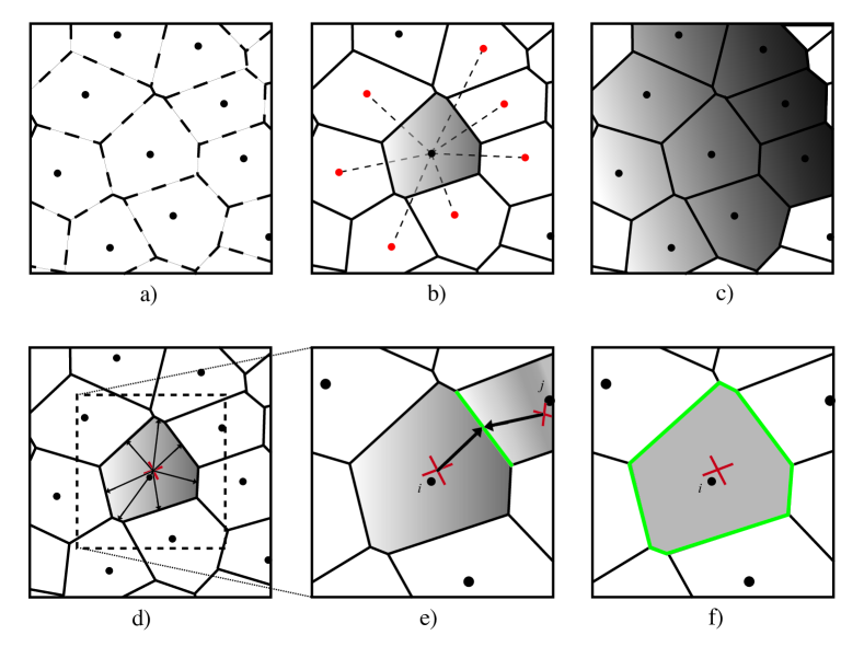
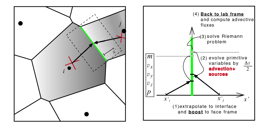
Figures 1 and 2 illustrate the mesh geometry and the basic steps of this inviscid numerical scheme implemented in AREPO. One additional point we have not explicitly discussed here for simplicity is the treatment of the mesh motion, as indicated in Fig. 2. This is incorporated into the scheme by evaluating all fluxes in the rest frame of the corresponding face, as described by Springel (2010). This requires appropriate boosts of the fluid states and the fluxes from the lab frame to the rest frame of each face, and back. For a Voronoi mesh, the face velocities are fully specified by the velocities of all the mesh generating points. The latter can be chosen freely in principle, but if they are set equal to the fluid velocities of the corresponding cells, a Lagrangian behavior and a manifestly Galilean-invariant discretization scheme is obtained in which the truncation error does not depend on the bulk velocity of the system.

Figure 1: Schematic representation of the mesh geometry and the MUSCL-Hancock integration scheme implemented in AREPO: a) TheVoronoi mesh is uniquely determined by the location of the mesh-generating points. b) A gradient estimate for all primitive variables is obtained from the immediate neighbors of a given cell. c) The gradient-estimation process is repeated for each cell in the domain and thus a piece-wise linear reconstruction is obtained for each primitive variable. d) The primitive variables are extrapolated toward each interface and evolved for half a time-step. e) For each face, a pair of extrapolated quantities for two neighboring cells $i$ and $j$ forms a local Riemann problem. f) The Riemann problem is solved for each face of a cell, yielding time-centered Godunov fluxes for the entire boundary of the control volume $V_{i}$ of cell $i$. These fluxes are used for updating the conserved quantities of the cell through Eq. (25).

Figure 2: Detailed description of the flux calculation with a Riemann solver in step e) of Fig. 1. For the case of a moving mesh, the standard MUSCL-Hancock method needs to be augmented with Galilean-boosts, as described by Springel (2010): (1) The extrapolation towards each interface is followed by a Galilean boost of the velocities to the rest frame of the face, and by a rotation of the coordinate axes. Each face is then treated as a one-dimensional discontinuity. Thus, the axes are oriented in the rotated frame such that the $x^{\prime}$-axis coincides with the normal to the face (left panel). (2) The primitive variables in the moving frame are evolved for half a time-step, including source terms if present (e.g. gravity or viscosity). (3) A one dimensional Riemann problem is solved at the interface. (4) The velocities are translated back to the lab frame and the advective fluxes are computed.

3.2 A MUSCL-Hancock Finite-Volume Scheme with Viscous Terms

A cell-centered, finite-volume solution of the NS equation can be written as

$$\mathbf{Q}_{i}^{n+1}=\mathbf{Q}_{i}^{n}-\Delta t\sum_{j}A_{ij}\hat{\mathbf{F}}_{\mathrm{adv},ij}^{n+1/2}-\Delta t\sum_{j}A_{ij}\hat{\mathbf{F}}_{\mathrm{diff},ij}^{n+1/2},$$ (29)

where we have retained the distinction between advective and viscous fluxes. As in the case of the Euler equations, the numerical method essentially consists of the problem of finding accurate time-centered numerical fluxes across each of the interfaces of a cell. How to do this in detail for the diffusive part of the fluxes has been the focus of numerous efficiency and stability analyses (see Puigt et al., 2010, for a detailed description).

Eq. (29) uses time-centered fluxes, obtained here with the two-step Hancock technique, as described above. Thus, for estimating both $\hat{\mathbf{F}}_{\mathrm{adv},ij}^{n+1/2}$ and $\hat{\mathbf{F}}_{\mathrm{diff},ij}^{n+1/2}$ a half time-step predictor stage is required. In the MUSCL-Hancock approach for inviscid flow, this step is carried out by linear reconstruction from each cell center to the interface, followed by solving a one-dimensional Riemann problem at the interface where the extrapolations meet. The traditional formulation of the Riemann problem and its solution are exclusive to hyperbolic differential equations and thus do not provide exact solutions for the NS equations. Since a general solution for the viscous Riemann problem does not exist, we will treat the viscous fluxes in Eq. (29) as a correction to the solution of an otherwise inviscid flow.

Our NS version of the MUSCL-Hancock scheme consists of the following three different stages (in addition to those described in Section. 3.1):

• Correct the MUSCL linear extrapolation of primitive variables by applying a viscous kick.

• Extrapolate the cell-centered gradients linearly and evolve them for half a time-step.

• Average the extrapolated velocity gradients at the interface and use them to estimate viscous fluxes.

To extrapolate the gradients from their cell-centered values to the interfaces, information about the higher-order derivatives of the primitive variables is needed. If gradients are assumed to vary linearly in space, an estimator for the Hessian matrix for each of the five primitive variables is sufficient. Evidently, enough information is contained in the cell-centered quantities to estimate both the local gradient $\nabla\phi$ and the Hessian $\mathbf{H}^{\phi}$ corresponding to a given scalar quantity $\phi$. However, estimating both of these simultaneously is significantly more difficult than estimating them one after the other. Therefore, we will effectively treat $\phi$ and $\nabla\phi$ as two independent fields that vary linearly in space, and this variation needs to be estimated from the mesh data through a suitably discretized differential operator.

As a simpler alternative to the gradient reconstruction approach, we briefly describe how one can use the gradients already available from the linear reconstruction step. In this approximation, a given quantity varies only linearly within the control volume, such that consistently evaluated gradients are piece-wise constant. This means that each interface represents a discontinuity in the gradient field $\nabla\phi$. Naively, one may think that the arithmetic average of both gradients that meet at a face is a good estimate for the gradient at the interface itself. However, on second thought, one realizes that both cells do no necessarily have the same weight if cells of different volume meet. Furthermore, the unweighted average of the two cell-centered values really represents the value at the midpoint of the two mesh-generating points, which, for a Voronoi mesh, can be substantially offset from the mid-point of the face. We therefore adopt the approach of Loh (2007), which consists in choosing one of the two gradients that meet at the interface, based on prior knowledge of the direction of the flow across the interface. Thus the three-stage scheme introduced above could be alternatively replaced by the simpler method:

• At the cell interface where two different gradients meet, choose the upwind gradient.

In either method, once we have an estimate of both viscous and advective fluxes, the time-step evolution of the conserved quantities $\mathbf{Q}_{i}$ is carried out as in Eq. (29). However, the approach (A-C) is preferable to the Loh (2007) scheme because it uses time-centered estimates for both $\hat{\mathbf{F}}_{\mathrm{adv},ij}^{n+1/2}$ and $\hat{\mathbf{F}}_{\mathrm{diff},ij}^{n+1/2}$, hence preserving the order of accuracy of the original inviscid scheme. We therefore now provide a more detailed description of the individual steps in this three-stage approach.

(A) Viscosity Kicks

Although Eq. (29) is written in an unsplit form, the predictor step is indeed operator split, evolving the advective and diffusive terms separately (e.g. Coirier & Powell, 1996). While our method for estimating the advective fluxes remains the MUSCL-Hancock scheme, the technique for estimating the diffusive fluxes is essentially contained in the estimation of the velocity gradients at each interface (see Coirier, 1994; Puigt et al., 2010, for a series of tests on different interface gradient estimates). Looking for better accuracy, we have chosen to couple these two otherwise independent procedures by correcting/biasing the linear extrapolation of the velocity field (stage $(I)$ in Section 3.1) with a viscous source term.

The benefit of carrying out a linear extrapolation to cell interfaces in primitive variables is the simplicity of the Galilean transformation needed to boost the quantities to the frame of a moving interface. Since the Galilean boost does not affect the mass and pressure of a given cell, only the local velocity field is transformed. In addition, adding force source terms to the equations of motion in primitive variable formulation is simpler, since these only couple to the momentum equations. Thus, a “viscous kick” can be applied to the velocity field in the half time-step evolution stage:

$$\Delta\mathbf{v}_{\mathrm{visc}}=\frac{\Delta t}{2}\left[\frac{\eta}{\rho}\nabla^{2}\mathbf{v}+\frac{\zeta+\frac{1}{3}\eta}{\rho}\nabla\left(\nabla\cdot\mathbf{v}\right)\right].$$ (30)

In this way, the subsequent linear extrapolation of primitive variables will already include viscosity effects to first order in time.

While working with numerical fluxes across interfaces requires velocity gradients, the use of cell-centered source terms in Eq. (30) calls for second order derivatives of the velocity field. Thus, in addition to the cell-centered velocity gradients $\nabla v_{x}$, $\nabla v_{y}$ and $\nabla v_{z}$, the cell-centered Hessian matrices $\mathbf{H}^{v_{x}}$, $\mathbf{H}^{v_{x}}$ and $\mathbf{H}^{v_{x}}$ are now needed. As we will see below, these matrices will be of use in more than one occasion, justifying the computational cost incurred to calculate them.

(B) Linear Extrapolation of Gradients

The linear reconstruction implemented in our MUSCL-Hancock approach essentially assumes that the gradient of a scalar quantity $\phi$ does not vary significantly across the spatial scale of a cell. For smooth flows, the gradients of two neighboring cells $\nabla\phi\Big{|}_{i}$ and $\nabla\phi\Big{|}_{j}$ will not differ significantly. Furthermore, in the presence of strong discontinuities, gradients on each side will be slope-limited, and therefore will not differ by much either. Hence, a first guess for the gradient at the interface between two cells is just the average of the cell-centered estimates at each side of the face

$$\widetilde{\nabla\phi}\Big{|}_{ij}=\frac{\langle\nabla\phi\rangle_{i}+\langle\nabla\phi\rangle_{j}}{2}.$$ (31)

However, as we pointed out earlier, the gradient average above is actually representative of the midpoint between the two cell centers $\mathbf{r}_{i}$ and $\mathbf{r}_{j}$, which in general does not lie close to the center of the face in a Voronoi mesh, and may in fact lie within a third cell. Unless gradients are assumed to vary within a cell, it will not be possible to assign the estimate to the center of the interface with any confidence.

Figure 3: Schematic representation of the double linear reconstruction proposed in this work compared to standard linear reconstruction and parabolic reconstruction.

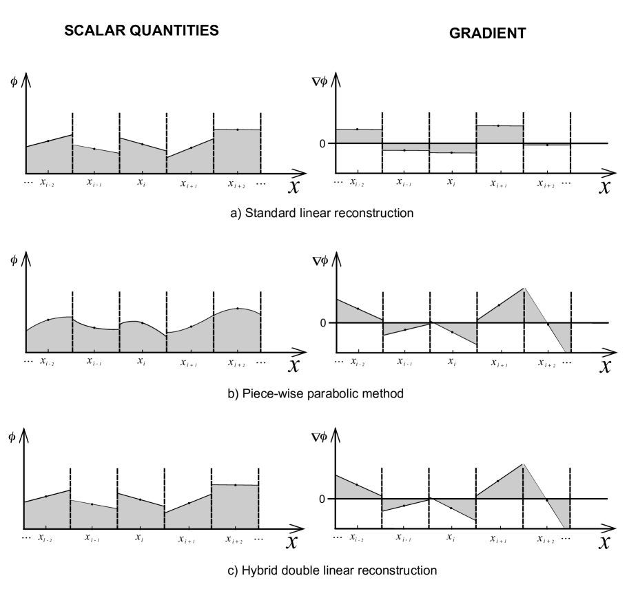
Let us assume that the scalar field $\phi(\mathbf{r})$ is infinitely differentiable and, consequently, so is its first derivative. Thus, we can Taylor expand both quantities to arbitrary order around a mesh generating point $\mathbf{r}_{0}$:

$$\begin{split}\phi(\mathbf{r})=&\phi(\mathbf{r}_{0})+\nabla\phi\Big{|}_{\mathbf{r}_{0}}(\mathbf{r}-\mathbf{r}_{0})\\ &+\frac{1}{2}(\mathbf{r}-\mathbf{r}_{0})^{T}\mathbf{H}^{\phi}\Big{|}_{\mathbf{r}_{0}}(\mathbf{r}-\mathbf{r}_{0})+\mathcal{O}(\mathbf{d}^{3})\end{split}$$ (32)

$$\begin{split}\nabla\phi(\mathbf{r})=&\nabla\phi\Big{|}_{\mathbf{r}_{0}}+\mathbf{H}^{\phi}\Big{|}_{\mathbf{r}_{0}}(\mathbf{r}-\mathbf{r}_{0})\\ &+\frac{1}{2}(\mathbf{r}-\mathbf{r}_{0})^{T}\mathbf{D}^{\phi}\Big{|}_{\mathbf{r}_{0}}(\mathbf{r}-\mathbf{r}_{0})+\mathcal{O}(\mathbf{d}^{3})\end{split}$$ (33)

where $\mathbf{H}^{\phi}$ is the Hessian matrix of the scalar quantity $\phi$ and $\mathbf{D}^{\phi}$ is a $3\times 3\times 3$ tensor containing the third-order derivatives of $\phi$ (i.e. $D_{abc}=\partial^{3}\phi/\partial x_{a}\partial x_{b}\partial x_{c}$). Truncating both Taylor expansions to first-order in $\mathbf{d}=\mathbf{r}-\mathbf{r}_{0}$, we see that we can obtain linear reconstructions for both the physical quantities and their gradients provided that we have numerical estimates for both the gradients and the Hessians at each mesh generating point.

We emphasize that a Taylor expansion is not equivalent to a polynomial data reconstruction. Indeed, it is desirable that reconstruction schemes are manifestly conservative, in the sense that the average of the reconstruction over the cell should be identical to the value of $\phi$ at the geometric center of the cell. This property of reconstruction schemes is sometimes referred to as $K$-exactness, meaning that if a polynomial reconstruction is cell-averaged over the mesh, the reconstruction procedure recovers the same polynomial. This condition is trivially satisfied for a linear reconstruction of the form $\phi(\mathbf{r})=\phi_{i}+\langle\nabla\phi\rangle_{i}(\mathbf{r}-\mathbf{s}_{0})$. However, higher-order reconstruction schemes require the use of zero-mean polynomials, which, beyond first-order, differ from the Taylor series (e.g. Colella & Woodward, 1984; Coirier & Powell, 1996).

The linear reconstruction of the scalar field $\phi$ and of the vector field $\nabla\phi$, treated as if they were independent quantities, effectively constitutes a hybrid method between standard linear reconstruction and fully K-exact second-order reconstruction, as illustrated in Figure 3. In this approximation, second derivatives are considered negligible for the spatial reconstruction of the primitive quantities, but they are still included for a more accurate estimate of the gradients near the cell interfaces. We also note, that in this way our numerical scheme reduces to that originally in AREPO (which is second-order-accurate) when the viscous fluxes are disabled.

Once an estimate for the Hessian matrix $\mathbf{H}^{\phi}\Big{|}_{\mathbf{r}_{0}}$ is available (Section 3.3), a linear extrapolation of the gradients from the cell centers to the interfaces can be obtained from

$$\widetilde{\nabla\phi}\Big{|}_{ij}=\langle\nabla\phi\rangle_{i}+\langle\mathbf{H}^{\phi}\rangle(\mathbf{f}_{ij}-\mathbf{r}_{i}),$$ (34)

which is a better approximation than Eq. (31). However, the time evolution of the gradients during a single step could be equally important as their spatial variation over the length scale of a cell, hence we also need to evolve them for half a time-step to obtain a time integration scheme that is consistent with the second-order accurate two-stage MUSCL-Hancock approach. In the latter, to extrapolate and evolve a scalar quantity $\phi$ we consider

$$\phi\Big{|}_{ij}=\phi_{i}+\nabla\phi\Big{|}_{\mathbf{r}_{0}}\left(\mathbf{f}_{ij}-\mathbf{s}_{i}\right)-\frac{\Delta t}{2}\left\langle\frac{\partial\phi}{\partial t}\right\rangle_{i}$$ (35)

where the time derivative of the quantity $\phi$ in the control volume of the $i$-th cell can be obtained from the primitive variable formulation of the Euler equations in tensor notation:

$$\partial_{t}W_{\alpha}+A_{\alpha\beta b}(\mathbf{W})\partial_{b}W_{\beta}=0.$$ (36)

Here sums over repeated indices are implied. Latin indices $a,b,c,d...$ take the values $1,2,3$ or $x,y,z$, while Greek indices $\alpha,\beta,\gamma,...$ take the values $1,2,3,4,5$ and are used to number the components of the primitive quantity vector ($W_{\alpha}=\rho,v_{x},v_{y},v_{z},P$ for $\alpha=1,2,3,4,5$, respectively). As with our previous notation, the indices $i,j$ and $k$ are reserved for labeling the mesh generating points and their associated cells.

Eq. (36) is an advection equation for the primitive variables. Analogously, to “advect” the gradients of the primitive variables from the cell center to the interface, we can ignore the viscous terms and derive an equation of motion for the spatial derivatives by differentiating Eq. (36):

$$\partial_{a}\partial_{t}W_{\alpha}+\left(\partial_{a}A_{\alpha\beta b}\right)\partial_{b}W_{\beta}+A_{\alpha\beta b}\partial_{a}\partial_{b}W_{\beta}=0,$$ (37)

where we can identify the Jacobian matrix of the primitive variables as $J_{\alpha a}\equiv\partial_{a}W_{\alpha}=W_{\alpha,a}$, and the Hessian tensor ($5\times 3\times 3$) of the primitive variables as $H_{\beta ba}\equiv\partial_{b}\partial_{a}W_{\beta}=W_{\beta,b,a}$. Therefore, the time derivative of each component of the primitive variable Jacobian matrix is

$$\partial_{t}J_{\alpha a}=B_{\alpha\beta ba}J_{\beta b}-A_{\alpha\beta b}H_{\beta ba},$$ (38)

where we introduced the rank-$4$ tensor $B_{\alpha\beta ba}\equiv\partial_{a}A_{\alpha\beta b}=A_{\alpha\beta b,a}$. Since $A_{\alpha\beta b}$ is a function of the primitive variables $W_{\alpha}$, the tensor $B_{\alpha\beta ba}$ can also be written as (see Appendix)

$$B_{\alpha\beta ba}=\frac{\partial A_{\alpha\beta b}}{\partial W_{\gamma}}\partial_{a}W_{\gamma},$$ (39)

and therefore its numerical estimate is given by the product of the exact derivatives $\partial A_{\alpha\beta b}/\partial W_{\gamma}$ (evaluated with values of the primitive variables at the center of the cell) and the (already available) numerical estimates for the gradients $\partial_{a}W_{\gamma}=J_{\gamma a}$. The second term on the right hand side of Eq. (38) is the product of the known coefficients $A_{\alpha\beta b}$ (evaluated at the center of the cell) and the numerical estimates of the Hessian tensor $H_{\beta ba}$.

Finally, with a numerical estimate of $H_{\beta ba}$ at hand (see Section 3.3), the extrapolated and half time-step evolved gradients of the velocity are (in analogy to Eq. 35):

$$\nabla v_{x}\Big{|}_{ij}=\langle\nabla v_{x}\rangle_{i}+\langle\mathbf{H}^{v_{x}}\rangle_{i}\left(\mathbf{f}_{ij}-\mathbf{s}_{i}\right)+\frac{\Delta t}{2}\left\langle\frac{\partial\nabla v_{x}}{\partial t}\right\rangle_{i},$$ (40)

with analogous expressions for $\nabla v_{y}\,|_{ij}$ and $\nabla v_{z}\,|_{ij}$. In Eq. (40), the term $\left\langle\partial\nabla v_{x}/\partial t\right\rangle_{i}$ is obtained from Eq. (38) with $\alpha=2$ and $a=1,2,3$.

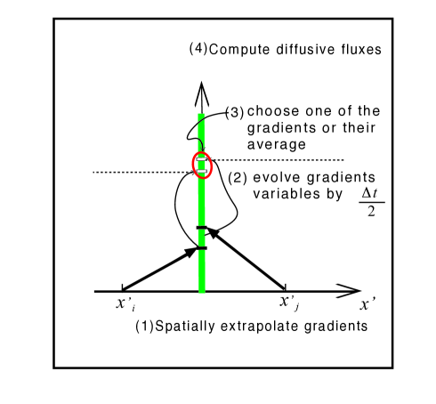
In Fig. 4, we show a sketch of the different steps involved in obtaining time-centered diffusive fluxes. We point out that taking the Hessian matrices of the velocity field to be identically zero is $not$ equivalent to the alternative scheme $(A^{\prime})$. The third term to the right hand side of Eq. (40) is still different from zero even if $H_{\beta ba}=0$ (Eq. 38) since, in general, $B_{\alpha\beta ba}J_{\beta b}\neq 0$. By advecting the gradients according to Eq. (38) we gain additional accuracy at no additional computational expense because the terms $B_{\alpha\beta ba}J_{\beta b}$ are known exactly (see Appendix), given the values of the primitive variables and their respective gradients at the center of each cell.

Figure 4: Sketch illustrating the individual steps involved in the extrapolation and half time-step evolution of the gradients, analogous to the advective flux calculation shown in Fig. 2. The different steps are: (1) spatial extrapolation of the gradients, followed by (2) a time advance by $\Delta t/2$ according to Eq. (35), and (3) an approximate evaluation right at the interface. In step (4), the viscous fluxes are determined by evaluating Eq. (22) with the values of the primitive variables and the velocity gradients at the interface.

(C) Viscous Flux Calculation

An accurate estimate of the viscous fluxes between two cells requires an accurate estimate of the velocity gradients at the interface. The gradient extrapolation method described above produces in general two different values of the velocity gradient that meet at the interface. This defines a general Riemann problem for the differential equation in Eq. (38) which is no longer a homogeneous hyperbolic differential equation. Therefore, attempting to solve this new Riemann problem for the spatial derivatives of the scalar quantities introduces a significant additional difficulty. For simplicity, we will assume that the differences between two gradient extrapolations meeting at an interface are small enough such that a simple arithmetic mean can be used. This assumption, of course, is valid only when the field of second derivatives is sufficiently smooth (see Section 3.3).

The time and area averaged flux across the face $i$-$j$ that moves with speed $\mathbf{w}$ is defined as

$$\begin{split}\hat{\mathbf{F}}_{ij}=\frac{1}{\Delta t}\frac{1}{A_{ij}}\int_{\Delta t}\int_{A_{ij}}&\left[\frac{}{}\mathbf{F}_{\mathrm{adv}}(\mathbf{U})-\mathbf{U}\mathbf{w}^{T}\right.\\ &\left.-\mathbf{F}_{\mathrm{diff}}(\mathbf{W,\partial\mathbf{W}/\partial{\mathbf{r}}})\frac{}{}\right]{\rm d}\mathbf{A}_{ij}\;{\rm d}t\\ \equiv\hat{\mathbf{F}}_{\mathrm{adv},ij}-\hat{\mathbf{F}}_{\mathrm{diff},ij}&~{}~{}.\end{split}$$ (41)

The numerical or Godunov estimate of these fluxes is chosen so that the analytic expressions for $\mathbf{F}_{\mathrm{adv}}(\mathbf{U})$ and $\mathbf{F}_{\mathrm{diff}}(\mathbf{W,\partial\mathbf{W}/\partial{\mathbf{r}}})$ are evaluated with numerical estimates of $\mathbf{U}$, $\mathbf{W}$ and $\partial\mathbf{W}/\partial\mathbf{r}$ at the centroid of the interface. The advective Godunov fluxes are

$$\hat{\mathbf{F}}_{\mathrm{adv},ij}=\left[\mathbf{F}_{\mathrm{adv}}(\mathbf{U}^{\mathrm{lab}}_{\mathrm{Riem}})-\mathbf{U}^{\mathrm{lab}}_{\mathrm{Riem}}\mathbf{w}^{T}\right]\hat{\mathbf{n}}_{ij},$$ (42)

where $\mathbf{U}^{\mathrm{lab}}_{\mathrm{Riem}}$ is the conserved variable vector at the centroid of the interface, as seen in the lab frame, obtained from the solution of a 1-D Riemann problem across the $i$-$j$ interface and along its normal. Multiplying by $\hat{\mathbf{n}}_{ij}$ is equivalent to projecting the flux matrix $\mathbf{F}_{\mathrm{adv}}$ (Eq. 3) along the normal of each face. The Godunov fluxes $\hat{\mathbf{F}}_{\mathrm{adv},ij}$ and $\hat{\mathbf{F}}_{\mathrm{diff},ij}$ are thus $5$-component vectors. The diffusive Godunov flux vector is obtained from the diffusive flux $5\times 3$ matrix

$$\begin{split}\mathbf{F}_{\mathrm{diff}}=\left[\begin{matrix}\\ 0\\ \Pi_{xx}\\ \Pi_{xy}\\ \Pi_{xz}\\ v_{x}\Pi_{xx}+v_{y}\Pi_{xy}+v_{z}\Pi_{xz}\\ \\ \end{matrix}\right.&\begin{matrix}\\ 0\\ \Pi_{yx}\\ \Pi_{yy}\\ \Pi_{yz}\\ \;\;\;v_{x}\Pi_{yx}+v_{y}\Pi_{yy}+v_{z}\Pi_{yz}\\ \\ \end{matrix}\\ \\ &\left.\begin{matrix}\\ 0\\ \Pi_{zx}\\ \Pi_{zy}\\ \Pi_{zz}\\ v_{x}\Pi_{zx}+v_{y}\Pi_{zy}+v_{z}\Pi_{zz}\\ \\ \end{matrix}\right]\\ \end{split}$$ (43)

where $\Pi_{ab}$ are the components of the viscous stress tensor $\mathbf{\Pi}$, which depend on the local value of the velocity and the velocity gradients. These components are:

$$\begin{array}[]{ccl}\Pi_{xx}&=&\cfrac{4}{3}\eta\partial_{x}v_{x}-\cfrac{2}{3}\eta\left(\partial_{y}v_{y}+\partial_{z}v_{z}\right)+\zeta\nabla\cdot\mathbf{v}\\ \Pi_{yy}&=&\cfrac{4}{3}\eta\partial_{y}v_{y}-\cfrac{2}{3}\eta(\partial_{z}v_{z}+\partial_{x}v_{x})+\zeta\nabla\cdot\mathbf{v}\\ \Pi_{zz}&=&\cfrac{4}{3}\eta\partial_{z}v_{z}-\cfrac{2}{3}\eta(\partial_{x}v_{x}+\partial_{y}v_{y})+\zeta\nabla\cdot\mathbf{v}\\ \\ \Pi_{xy}&=&\Pi_{yx}=\eta\left(\partial_{y}v_{x}+\partial_{x}v_{y}\right)\\ \\ \Pi_{yz}&=&\Pi_{zy}=\eta\left(\partial_{z}v_{y}+\partial_{y}v_{z}\right)\\ \\ \Pi_{zx}&=&\Pi_{xz}=\eta\left(\partial_{x}v_{z}+\partial_{z}v_{x}\right)\\ \end{array}$$ (44)

Just like with the advective fluxes, the flux tensor (Eq. 43) must be projected onto the normal $\hat{\mathbf{n}}_{ij}$ of each $ij$-interface to obtain the 5-component vector

$$\hat{\mathbf{F}}_{\mathrm{diff},ij}=\mathbf{F}_{\mathrm{diff}}\left(\mathbf{W}^{\mathrm{lab}}_{\mathrm{Riem}},\left(\partial\mathbf{W}/\partial\mathbf{r}\right)^{\mathrm{lab}}_{\mathrm{approx}}\right)\hat{\mathbf{n}}_{ij},$$ (45)

where $\mathbf{W}^{\mathrm{lab}}_{\mathrm{Riem}}$ is the primitive variable vector at the centroid of the interface, as seen in the lab frame (whose associated conserved variables are $\mathbf{U}^{\mathrm{lab}}_{\mathrm{Riem}}$ in Eq. 42). The spatial derivatives $\left(\partial\mathbf{W}/\partial\mathbf{r}\right)^{\mathrm{lab}}_{\mathrm{approx}}$ correspond to our extrapolate-and-average scheme for linearly varying gradients. As with $\mathbf{W}^{\mathrm{lab}}_{\mathrm{Riem}}$, we are interested in estimates of $\partial\mathbf{W}/\partial\mathbf{r}$ at the centroid of the face. For both these quantities, only the velocity and its spatial derivatives are relevant when viscous fluxes are calculated.

3.3 Hessian Estimation

In analogy to the gradient calculation for Voronoi meshes discussed by Springel (2010), here we discuss the estimates of the cell-centered Hessian matrices for each of the primitive variables $W_{\alpha}$. To this end, let us consider a vector field $\mathbf{u}$ that varies approximately linearly with distance as $\mathbf{u}\approx\mathbf{u}_{i}+\mathbf{h}\left(\mathbf{r}-\mathbf{r}_{i}\right)$ near $\mathbf{r}_{i}$. Up to linear order, the first derivative of $\mathbf{u}$ is simply $\mathbf{h}$. The volume-average of the spatial derivatives of $\mathbf{u}$ in the vicinity of $\mathbf{r}_{i}$ is

$$\begin{split}V_{i}\left\langle\frac{\partial\mathbf{u}}{\partial\mathbf{r}}\right\rangle_{i}=&\int_{V_{i}}\frac{\partial\mathbf{u}}{\partial\mathbf{r}}\,{\rm d}V\\ =&\int_{\partial V_{i}}\mathbf{u}\,{\rm d}\mathbf{A}\\ =&\sum_{j\neq i}\int_{A_{ij}}\left[\mathbf{u}_{i}+\mathbf{h}(\mathbf{r}-\mathbf{r}_{i})\right]\frac{\mathbf{r}_{j}-\mathbf{r}_{i}}{r_{ij}}\,{\rm d}A,\end{split}$$ (46)

where we have assumed that the linear approximation is valid up to all the neighboring mesh generating points $\mathbf{r}_{j}$. It is straightforward to verify that the average matrix $\langle\partial\mathbf{u}/\partial\mathbf{r}\rangle_{i}$ can be written as

$$\begin{split}\left\langle\frac{\partial\mathbf{u}}{\partial\mathbf{r}}\right\rangle_{i}=&\frac{1}{V_{i}}\sum_{j\neq i}A_{ij}\left(\frac{\mathbf{u}_{i}+\mathbf{u}_{j}}{2}\otimes\widehat{\mathbf{n}}_{ij}\right)\\ &-\frac{1}{V_{i}}\sum_{j\neq i}A_{ij}\left(\mathbf{h}\,\mathbf{c}_{ij}\otimes\frac{\mathbf{r}_{ij}}{r_{ij}}\right).\end{split}$$ (47)

Writing the vector product $\left(\mathbf{A}\,\mathbf{u}\right)\otimes\mathbf{v}$ in tensor form (where $\mathbf{A}$ is a $n\times n$ square matrix and $\mathbf{u}$ and $\mathbf{v}$ are vectors of dimension $n$), it is easy to prove the identity $A_{ac}u_{c}v_{b}=A_{ac}v_{c}u_{b}+\varepsilon_{bfc}\varepsilon_{fde}u_{d}v_{e}A_{ac}$. Equivalently, going back to vector notation, we have $\left(\mathbf{A}\,\mathbf{u}\right)\otimes\mathbf{v}=\left(\mathbf{A}\,\mathbf{v}\right)\otimes\mathbf{u}+\left(\mathbf{u}\times\mathbf{v}\right)\times\mathbf{A}$, where, for simplicity, we used vector notation to denote a “cross product” between a vector and a matrix.

Therefore, the second term on the right hand side of Eq. (47) can be written as

$$\begin{split}\sum_{j\neq i}A_{ij}\left(\mathbf{h}\,\mathbf{c}_{ij}\otimes\frac{\mathbf{r}_{ij}}{r_{ij}}\right)=&\sum_{j\neq i}A_{ij}\left(\mathbf{h}\,\mathbf{r}_{ij}\otimes\frac{\mathbf{c}_{ij}}{r_{ij}}\right)\\ &+\sum_{j\neq i}\left(A_{ij}\mathbf{c}_{ij}\times\frac{\mathbf{r}_{ij}}{r_{ij}}\right)\times\mathbf{h}~{}~{}.\end{split}$$ (48)

Here, the second term on the right hand side vanishes identically, because

$$\begin{split}\sum_{j\neq i}\left(A_{ij}\mathbf{c}_{ij}\times\frac{\mathbf{r}_{ij}}{r_{ij}}\right)\times\mathbf{h}=&\left\{\int_{\partial V_{i}}\left(\mathbf{r}-\frac{\mathbf{r}_{i}+\mathbf{r}_{j}}{2}\right)\times{\rm d}\mathbf{A}\right\}\times\mathbf{h}\\ =&\left\{\int_{V_{i}}\nabla\times\left(\mathbf{r}-\frac{\mathbf{r}_{i}+\mathbf{r}_{j}}{2}\right){\rm d}V\right\}\times\mathbf{h}\\ =&~{}0~{}~{}.\end{split}$$ (49)

On the other hand, the first term on the right hand side of Eq. (48) can be rewritten by means of the replacement $\mathbf{h}\,\mathbf{r}_{ij}=-\mathbf{h}\,(\mathbf{r}_{j}-\mathbf{r}_{i})=\mathbf{u}_{i}-\mathbf{u}_{j}$. Finally, identifying the vector $\mathbf{u}_{i}$ with the gradient $\langle\nabla\phi\rangle_{i}$ of a scalar quantity $\phi$, and the matrix $\langle\partial\mathbf{u}/\partial\mathbf{r}\rangle_{i}$ with the cell-averaged Hessian matrix $\langle\mathbf{H}^{\phi}\rangle_{i}$, Eq. (48) takes the form

$$\begin{split}\left\langle\mathbf{H}^{\phi}\right\rangle_{i}=&\frac{1}{V_{i}}\sum_{j\neq i}A_{ij}\left\{-\left(\frac{\langle\nabla\phi\rangle_{i}+\langle\nabla\phi\rangle_{j}}{2}\right)\otimes\frac{\mathbf{r}_{ij}}{r_{ij}}\right.\\ &\left.+\left(\frac{}{}\langle\nabla\phi\rangle_{j}-\langle\nabla\phi\rangle_{i}\right)\otimes\frac{\mathbf{c}_{ij}}{r_{ij}}\right\}.\end{split}$$ (50)

The most noteworthy characteristic of this expression is that it is purely algebraic and explicit in nature. That is, the Hessian matrix of $\phi$ is simply a linear combination of the neighboring gradients in which the coefficients are predetermined quantities that depend only on the local mesh geometry. Each one of those neighboring gradients is, at the same time, a linear combination of its immediate neighbors’ scalar quantities (see Eq. 21 of Springel, 2010). Therefore, the Hessian estimate of Eq. (50) is a weighted linear combination of scalars from its immediate neighbors and from its neighbors’ neighbors and, as such, it implicitly employs a larger stencil than the one used for the gradients.

3.4 Slope-Limiting the Hessians

It is well known that higher-order reconstruction schemes are prone to produce spurious oscillations in the vicinity of steep gradients, unless this is prevented by appropriate slope limiter methods (Toro, 2009). These non-linear corrections in the data reconstruction procedure prevent overshoots and allow for true discontinuities in the solutions. So far, we have discussed how to estimate second derivatives from first derivatives, which in turn are already reconstruction estimates obtained from the scalar physical quantities. Potential irregularities in the second derivative fields can lead to spurious oscillations and unphysical values of the viscous stress tensor at the cell boundaries. To alleviate this problem, we enforce local monotonicity of each component of the gradients, which is equivalent to smoothing out the Hessian estimates. In practice, this is achieved by replacing the Hessian matrix by a ‘slope limited’ version

$$\overline{\left\langle\mathbf{H}^{\phi}\right\rangle_{i}}=\mathbf{A}_{i}\left\langle\mathbf{H}^{\phi}\right\rangle_{i}$$ (51)

with

$$\mathbf{A}_{i}=\begin{pmatrix}\alpha_{i}^{x}&0&0\\ 0&\alpha_{i}^{y}&0\\ 0&0&\alpha_{i}^{z}\end{pmatrix}\;\;\;\;\;\;\;\;\;\;\;\;\;\;\;\text{and where}\;\;\;\alpha_{i}^{a}=\mathrm{min}\left(1,\psi^{a}_{ij}\right)$$ (52)

are the slope limiters $0\leq\alpha_{i}^{a}\leq 1$ for each direction $x$, $y$ and $z$. This MINMOD-type slope-limiting method is readily applicable for irregular meshes. The quantities $\psi^{a}_{ij}$ are defined as

$$\psi^{a}_{ij}=\left\{\begin{array}[]{lcr}\left(\langle\partial_{a}\phi\rangle_{i}^{\mathrm{max}}-\langle\partial_{a}\phi\rangle_{i}\right)/\Delta\left(\partial_{a}\phi\right)_{ij}&&\Delta\left(\partial_{a}\phi\right)_{ij}>0\\ \left(\langle\partial_{a}\phi\rangle_{i}^{\mathrm{min}}-\langle\partial_{a}\phi\rangle_{i}\right)/\Delta\left(\partial_{a}\phi\right)_{ij}&&\Delta\left(\partial_{a}\phi\right)_{ij}<0\\ 1&&\Delta\left(\partial_{a}\phi\right)_{ij}=0\end{array}\right.$$ (53)

where the $\Delta\left(\partial_{a}\phi\right)_{ij}$ are the components of the vector $\Delta\left(\nabla\phi\right)_{ij}=\langle\mathbf{H}^{\phi}\rangle_{i}(\mathbf{f}_{ij}-\mathbf{s}_{i})$, i.e. the estimated change in the gradient $\nabla\phi$ between the centroid $\mathbf{f}_{ij}$ of the cell and the center of cell $i$. The quantities $\langle\partial_{a}\phi\rangle_{i}^{\mathrm{max}}$ and $\langle\partial_{a}\phi\rangle_{i}^{\mathrm{min}}$ are the maximum and minimum of the $a$-th component of the cell-centered gradient estimates among all neighboring cells of cell $i$, including $i$ itself.

To our knowledge, the slope-limiting technique has not been applied to the second derivatives before. However, its purpose is equivalent to the “flattening” procedure near shocks carried out by Colella & Woodward (1984) for parabolic reconstruction. In our approach, the suppression of oscillations near shocks is exclusively handled by the limitation of the gradients, since the reconstruction of hydrodynamic quantities is only of linear order. Thus, the Hessian limitation procedure serves the sole purpose of guaranteeing a smooth variation of the gradients and avoiding spuriously large viscous fluxes. Future improvements of the present method could however also employ these second derivatives for higher-order reconstructions of the scalars.

3.5 Time integration and time-step criterion

Because of the more complex mathematical properties of the NS equations compared with the Euler equations, obtaining a rigorous analytic expression analogous to the CFL stability criterion for the allowed time step size is not possible. However, MacCormack & Baldwin (1975) obtained an approximate semi-empirical stability criterion when advective, viscous and heat diffusion terms are considered. When there is no heat flux, the time-step criterion can be written as (e.g. Kundu & Cohen, 2008)

$$\Delta t\leq\frac{\sigma\Delta t_{\mathrm{CFL}}}{1+2/\{\mathrm{Re}\}_{i}},$$ (54)

where $\Delta t_{\mathrm{CFL}}$ is the standard CFL-criterion time-step except for the Courant-Friedrichs-Levy coefficient, which is absorbed into a “safety factor” $\sigma$ (usually $\approx 0.9$). In Eq. (54), the cell Reynolds number $\{\mathrm{Re}\}_{i}$ is

$$\{\mathrm{Re}\}_{i}=\frac{\rho|\mathbf{v}_{i}^{\prime}|R_{i}}{\eta},$$ (55)

where $\mathbf{v}_{i}^{\prime}$ is the velocity of the gas relative to the motion of the grid and $R_{i}$ is the effective radius of the cell, calculated as $R_{i}=(3V_{i}/4\pi)^{1/3}$ from the volume of a cell (or as $R_{i}=(A_{i}/\pi)^{1/2}$ from the area in 2D). Similar approaches to derive an appropriate NS time-step have also been described by Mavriplis & Jameson (1990) and Coirier & Powell (1996).

The numerical integration scheme we employ is time unsplit, that is, advective and diffusive fluxes are applied simultaneously during each hydrodynamic time-step and not sequentially (Eq. 29). The prediction stage, on the other hand, is operator-split, since the advective and diffusive terms are computed almost independently of each other. This is in part due to the nature of the standard one-dimensional Riemann problem, whose solutions – strictly speaking – are only valid for the hyperbolic Euler problem, but are not solutions to the full NS equations with their additional parabolic terms. The validity of this approach ultimately relies on the assumption that the viscous terms in the NS equations are typically small perturbations to the Euler equations.

4 Numerical Test Results

To test the performance of AREPO when our new treatment of viscous fluxes is included, we have carried out a number of test simulations for physical situations with known analytic or quantitative solutions. Usually, the problems with known exact solutions are either of self-similar type or have symmetries that make the non-linear term proportional to $(\mathbf{v}\cdot\nabla)\mathbf{v}$ vanish identically. Owing to these limitations, numerical simulations of situations with experimentally well-established behavior, such as flow past a circular cylinder, have become common-place in testing the performance of NS codes. We will therefore also carry out such qualitative benchmarks, besides looking at a few simple problems with analytic solutions.

Figure 5: Diffusion of a vortex sheet. The two panels show the velocity $u$ along the $x$-axis (left panel), and the vorticity (right panel), at times $t=0$, 0.1, 0.2, 0.4, 0.8, $1.6$ and $3.2$ (from black to red), for a dynamic viscosity coefficient $\mu=\nu\rho=0.005$. The solid lines are given by the analytic solution described by Eqs. (57), while the solid circles are all 2500 cell-centered velocity and vorticity values of the initially Cartesian $50\times 50$ mesh. Note that the simulation is started with a sharp discontinuity in velocity and thus the $\delta$-function vorticity field is initially unresolved. If the mesh would remain exactly Cartesian, the diffusion of vorticity would actually be suppressed in this case. Nevertheless, the small asymmetries introduced by the moving mesh trigger the diffusion regardless of the initially unresolved setup, and the time-dependent numerical result closely follows the expected exact solution.

(a) $t=0.0$

(b) $t=0.06$

(c) $t=0.6$

(d) $t=1.8$

Figure 6: Time evolution of the mesh geometry and the velocity field for a diffusing vortex sheet test. As the vorticity spreads from the center of the domain to the upper and lower boundaries, the mesh adapts to the continuous change in velocity until its original Cartesian structure disappears entirely. The color table (from blue to red) corresponds to the range between $u=-1.0$ and $u=1.0$ in linear scale.

4.1 Diffusion of a Vortex Sheet

A simple problem of laminar flow in the presence of viscosity is given by the vortex sheet diffusion test. In this problem, the initial velocity field at $t=0$ is given by $\mathbf{v}=(u,0,0)$ with $u=1$ for $y>0$ and $u=-1$ for $y<0$. Because of the symmetry of the problem, the NS equations reduce to a 1D diffusion equation

$$\frac{\partial u}{\partial t}=\nu\frac{\partial^{2}u}{\partial^{2}y},$$ (56)

with solution (e.g. Kundu & Cohen, 2008)

$$u=\mathrm{erf}\left[\frac{y}{2\sqrt{\nu t}}\right]\;\;\;\;\;\;\;\;\;\;\omega=\frac{\partial u}{\partial y}=\frac{e^{-y^{2}/4\nu t}}{\sqrt{\pi\nu t}}.$$ (57)

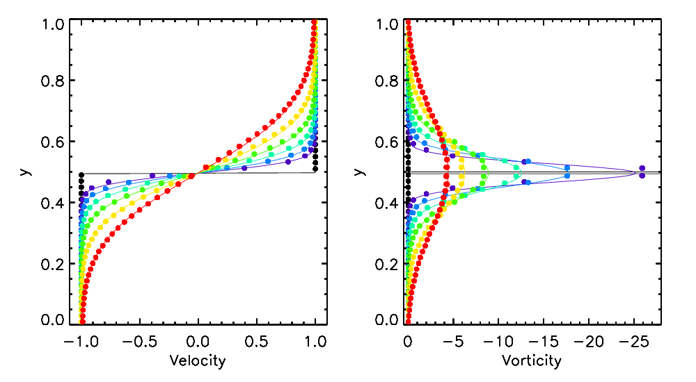
In Figure 5, we show the time evolution we obtain for a two-dimensional simulation domain with initially uniform pressure and density ($\rho=P=1$), and with a velocity field given by $\mathbf{v}=({\rm sgn}(y),0,0)$. The mesh generating points were distributed regularly at the initial time to produce a Cartesian mesh. As the system evolves, the velocity and the vorticity fields as a function of time and vertical coordinate $y$ follow the exact solution remarkably well. It is worth pointing out that the initial singularity in the vorticity field is unresolved numerically (and thus appears as being uniformly zero throughout the domain), since the system is started with an exact sharp discontinuity. Static, perfectly aligned meshes with slope limitation techniques will typically maintain this unresolved vorticity and thus no diffusion will proceed unless some numerical perturbations are seeded that break the mesh alignment of the initial state (a common way to overcome this difficulty is to start the system according to Eq. (57) at $t>0$ such that there is initial vorticity). However, the moving mesh of AREPO “sees” a non-zero velocity gradient as soon as the upper and lower halves of the domain become unaligned with respect to each other. This happens because, as soon as a cell shifts its position, the number of its neighbors that have a drastically different velocity increases and so does the “statistical weight” of the discontinuity. At this point, the slope-limiting technique, which had ignored the discontinuity in the perfectly aligned mesh, now identifies the local variation as “real” and the vorticity field is “detected”.

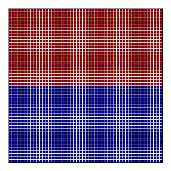
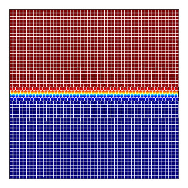
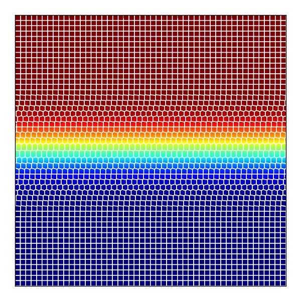
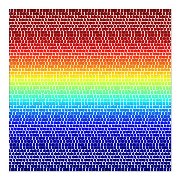
Fig. 6 shows the corresponding two-dimensional velocity field of the diffusing vortex sheet test at four different times, together with the geometry of the underlying Voronoi mesh. The mesh geometry nicely shows how the cells transform from a Cartesian configuration to an unstructured mesh, while the velocity field evolves from a piece-wise constant state with a central discontinuity to a smoothly varying shear flow due to the effects of viscosity.

4.2 Diffusion of a Gaussian Vortex

The two-dimensional circular velocity distribution corresponding to an irrotational vortex of circulation $\Gamma$ is

$$v_{\theta}=\frac{\Gamma}{2\pi R},$$ (58)

where the vorticity $\omega=|\nabla\times\mathbf{v}|=(1/R)\partial(R\,v_{\theta})/\partial R$ is zero everywhere except at the origin ($\omega=\delta(R)$, i.e. a vortex line). In a viscous fluid, this velocity profile has to be sustained by a point source of vorticity at the origin (e.g. an infinitely thin rotating cylinder) otherwise the vortex line will decay in a similar way as the vortex sheet in the previous example. If the velocity at the origin is set impulsively to zero, the subsequent evolution of the azimuthal velocity is given by

$$v_{\theta}(R,t)=\frac{\Gamma}{2\pi R}\left[1-e^{-R^{2}/4\nu t}\right]~{}~{},$$ (59)

while the vorticity $\omega=\left[\nabla\times(v_{\theta}\hat{\bm{\theta}})\right]\cdot\hat{\mathbf{z}}$ evolves as

$$\omega=-\frac{\Gamma}{4\pi\nu t}e^{-R^{2}/4\nu t}$$ (60)

and the Laplacian of the velocity field is

$$|\nabla^{2}\mathbf{v}|=\frac{\Gamma}{2\pi}\frac{R}{(2\nu t)^{2}}e^{-R^{2}/4\nu t}\hat{\bm{\theta}}~{}~{}.$$ (61)

Because of its geometry, this problem is significantly more challenging than the vortex sheet test considered above and cannot be impulsively started at precisely $t=0$. Besides the initial singularity in the vorticity field, the velocity field is divergent as we approach the origin. In addition, it is not possible to capture the azimuthal velocity field when the distance from the origin is comparable to the grid resolution. At the same time, the azimuthal velocity field is challenging for the boundary conditions, because the problem is self-similar in nature and therefore natural boundaries do not exist. These problems did not exist for the vortex-sheet problem, which is of one-dimensional nature. Nevertheless, evolving the system from an initial time $t>0$ minimizes most of these complications. In addition, we extend the computational domain far beyond the region of interest, such that boundaries become essentially irrelevant during the timespan of the numerical solution.

We setup a Cartesian mesh ($100\times 100$) with an imposed initial velocity profile of

$$v_{\theta,0}=\frac{\Gamma}{2\pi R}\left[1-\exp\left(-\frac{R^{2}}{4\nu t_{0}}\right)\right]\;\;\;\;\;\text{ with }\nu=\frac{\mu}{\rho},$$ (62)

corresponding to a Gaussian vortex that we center in the middle of the domain, which extends over the range $[0,40]\times[0,40]$, and thus accommodates a radial range from $R=0$ to $R=20$. The adopted physical parameters are $t_{0}=10$, $\mu=0.08$, $\Gamma=1.0$, and the initial density field is constant with $\rho=1$. The pressure field, however, is not uniform because the fluid is not started from rest. We obtain the correct pressure profile from the radial component of the equation of motion:

$$-\frac{v_{\theta}^{2}}{R}=-\frac{1}{\rho}\frac{{\rm d}P}{{\rm d}R},$$

and thus the initial pressure profile is

$$\begin{split}P_{\mathrm{init}}=P_{0}-\frac{\Gamma^{2}\rho}{4\pi^{2}}\left\{\frac{1}{2R^{2}}e^{-R^{2}/(2\nu t_{0})}\left[e^{R^{2}/(4\nu t_{0})}-1\right]^{2}\right.\\ \left.+\frac{1}{4\nu t_{0}}\left(\mathrm{Ei}\left(-\frac{R^{2}}{2\nu t_{0}}\right)-\mathrm{Ei}\left(-\frac{R^{2}}{4\nu t_{0}}\right)\right)\right\}~{}~{},\end{split}$$

where $P_{0}$ is an integration constant. The precise value of $P_{0}$ is irrelevant for the similarity solution presented here, because it is obtained for incompressible flow. In our numerical experiments (which are compressible), we set $P_{0}$ such that $P=1$ at $R=0$.

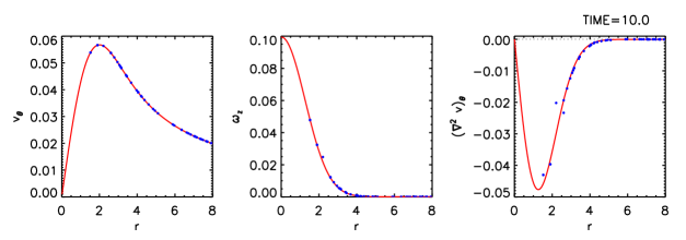
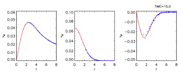
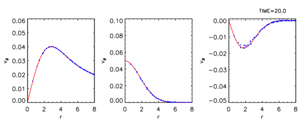
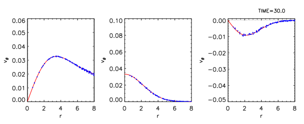
Fig. 7 shows the time evolution of the velocity field, the vorticity field and the Laplacian field for a Gaussian vortex started on an initially Cartesian mesh. We find not only that the velocity evolves as expected based on the similarity solution, but the first and second derivatives also show excellent agreement with the analytic expectations. These results validate both the space- and time-accuracy of our viscous integration scheme, as well as the accuracy with which the second derivatives are estimated.

Figure 7: Time evolution of a diffusing Gaussian vortex. For each time (as labeled), we show the azimuthal velocity profile $v_{\theta}(R)$, the vorticity profile $\omega(R)$ and the Laplacian profile $\nabla^{2}v_{\theta}$, as computed by AREPO (blue points; only a random $10\%$ of the total shown) and compare it to the corresponding analytic expressions (solid red lines).

(a) Plane Poiseuille flow

(b) Plane Couette flow

Figure 8: Impulsively started plane Poiseuille and Couette flows as a function of time. a) Time evolution of the horizontal velocity profile versus vertical distance. Solid curves represent the analytic solutions of Eqs. (63) to (65) for $U=0$ and ${\rm d}p/{\rm d}x=-0.05$, at ten different times (time increasing from black to red). The data points correspond to all the cell-centered values of velocity along $x$ for a $50\times 50$ simulation started from rest. b) Time evolution of the horizontal velocity profile versus vertical distance. Solid curves represent the analytic solutions in Eqs. (63) to (65) for $U=0.1$ and ${\rm d}p/{\rm d}x=0$ at eight different times (time increasing from black to red). The data points correspond to all the cell-centered values of velocity along $x$ for a $50\times 50$ numerical simulation started from rest.

(a) $t=0.1$

(b) $t=0.9$

(c) $t=2.5$

(d) $t=5.7$

Figure 9: Time evolution of the mesh geometry and the velocity for flow between parallel plates. The horizontal velocity field $u$ for plane Poiseuille flow is rendered at four different times. The evolution of the velocity field (see Fig 8(a)) is accompanied by the evolution of the mesh from an initially Cartesian set up (top-left panel) to a fully unstructured grid by the time the flow has reached steady state (bottom-right panel). The (linear ) color scale ranges from blue ($u=0$) to red ($u=0.12$).

4.3 Plane Poiseuille and Couette Flows

Next, we consider impulsively-started plane Poiseuille and Couette flows where a fluid between two parallel plates is initially at rest, and then, suddenly, either pressure gradients or plate motions are applied. The time-dependent solution has the form $\mathbf{v}=(u(y,t),0,0)$, where the horizontal velocity can be decomposed into steady and time-dependent parts, $u(y,t)=u_{0}(y)+\widetilde{u}(y,t)$. In the presence of a pressure gradient and an upper plate moving at constant speed $U$, the steady state solution is the well-known expression

$$u_{0}(y)=\frac{yU}{b}-\frac{y}{2\mu}\frac{{\rm d}p}{{\rm d}x}\left(b-y\right),$$ (63)

for which the special cases $U=0$ and ${\rm d}p/{\rm d}x=0$ are commonly known as plane Poiseuille flow and plane Couette flow, respectively.

The time dependent component $\widetilde{u}(y,t)$ is a solution of Eq. (56), subject to the initial condition $\widetilde{u}(y,0)=-u_{0}(y)$ and the boundary conditions $\widetilde{u}=0$ at $y=0$ and $y=b$. By separation of variables, the general solution is (e.g Graebel, 2007)

$$\widetilde{u}(y,t)=\sum_{n=1}^{\infty}A_{n}e^{-n^{2}\pi^{2}\nu t/b^{2}}\sin\frac{n\pi y}{b},$$ (64)

where the coefficients $A_{n}$ are determined by the initial condition

$$A_{n} =-\cfrac{\int_{0}^{b}u_{0}(y)\sin\frac{n\pi y}{b}{\rm d}y}{\int_{0}^{b}\sin^{2}\frac{n\pi y}{b}{\rm d}y}$$ (65)

$$=-\frac{2U(-1)^{n}}{n\pi}-\frac{2}{b\mu}\frac{{\rm d}p}{{\rm d}x}\left(\frac{b}{n\pi}\right)^{3}\left[1-(-1)^{n}\right]~{}~{}.$$ (66)

Figure 10: Schematic representation of (a) reflective and (b) non-slip boundaries within the computational domain. After the spatial and temporal extrapolation steps in the MUSCL-Hancock method (panel e) in Figure 1), the Riemann problem is solved as elsewhere in the domain but with the boundary-side cell mimicking the gas side with either one velocity component – the normal one – reversed (reflection) or all three (non-slip).

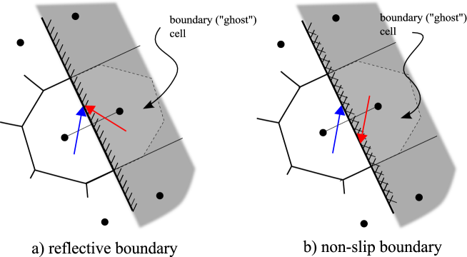
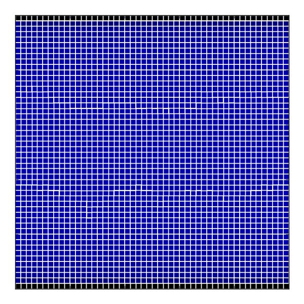
The numerical setup for this problem is straightforward. We produce a Cartesian mesh in the range $[0,1]\times[0,1]$ with a resolution of $50\times 50$. The fluid is originally at rest and its density and pressure are given by $\rho=P=1$. The equation of state is that of an ideal gas with adiabatic index $5/3$. To represent the plates, the uppermost and lowermost rows of cells are replaced by “solid boundaries“ at which the no-slip condition is enforced, i.e. $v_{x}=v_{y}=0$ (see Fig. 10). Moving solid boundaries are straightforward to implement with a Voronoi tessellation mesh. A solid surface can be constructed as a series of mesh-generating point pairs, one on each side of the surface, such that the common interface – equidistant to both points – defines the boundary locally (see Serrano & Español, 2001 and Springel, 2010). The Voronoi cell on the side of the “solid” object can regarded as “a ghost cell within the domain”. That is, this cell is part of the domain discretization process and is tessellated/updated as any other normal gas cell. However, when solving the Riemann problem at the local interface between a “solid” cell and a real gas cell, boundary conditions are imposed in the same way as boundary conditions on the outer box are imposed. For perfectly reflecting boundaries, the normal component of the velocity is reflected in the “solid side” or “outside region” of the interface. For non-slip boundaries, the entire velocity vector is reflected, such that the velocity at the interface is zero (Figure 10).

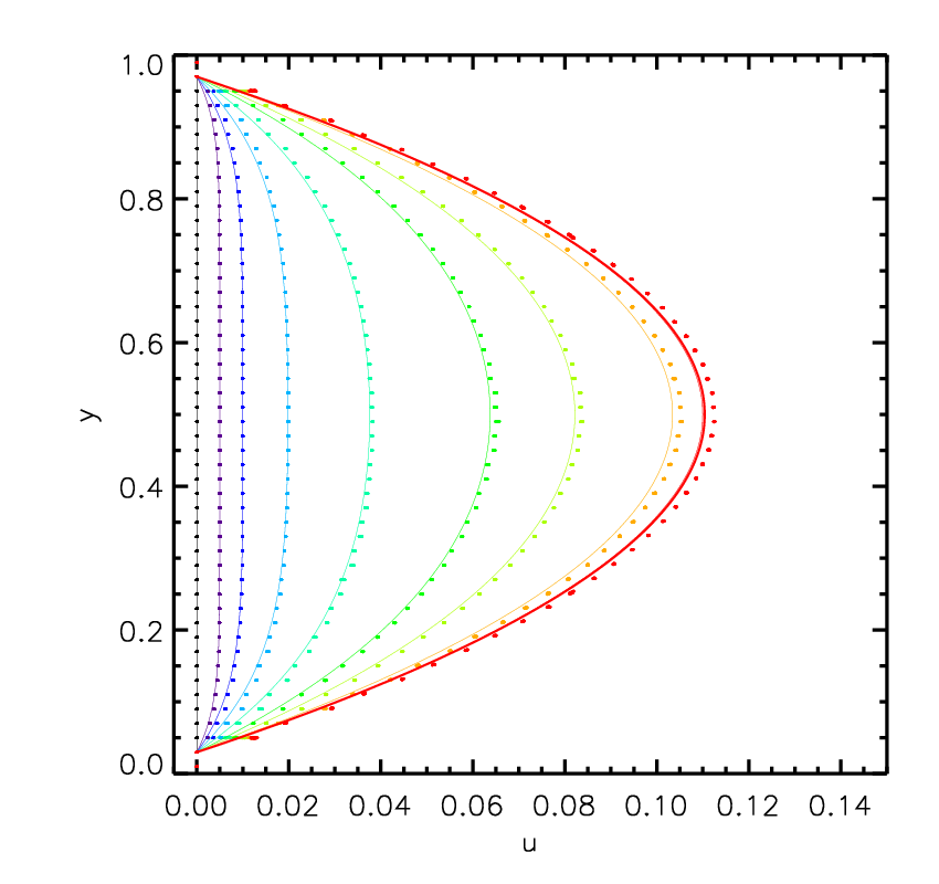
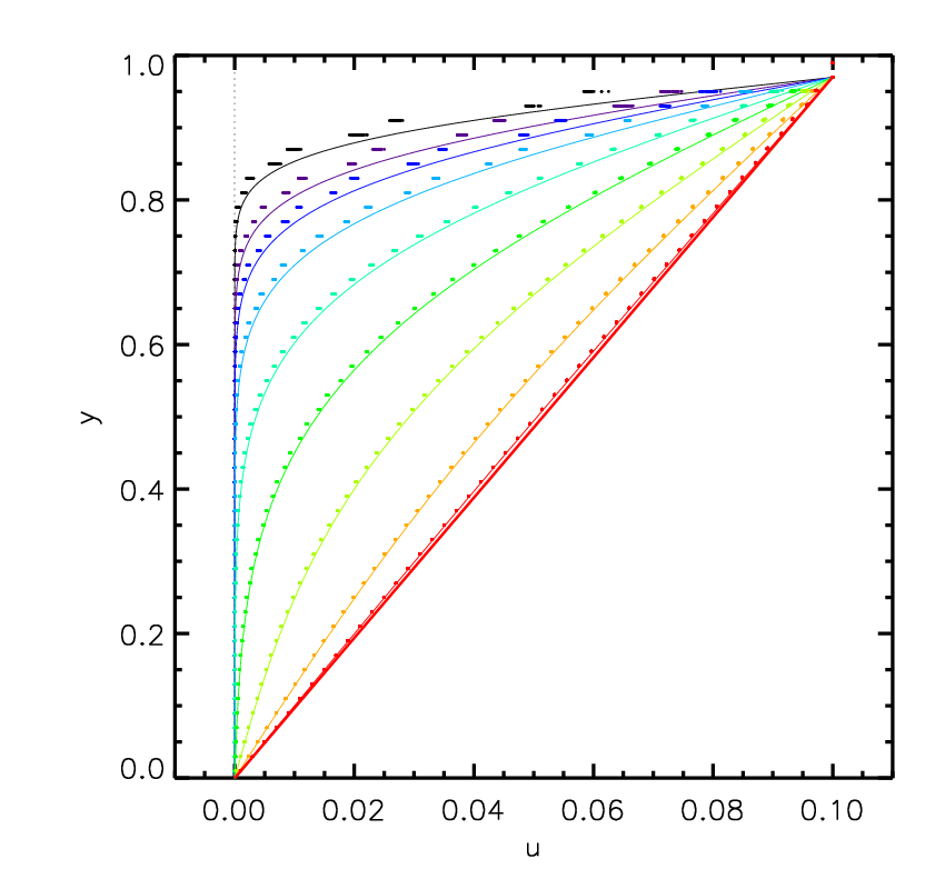
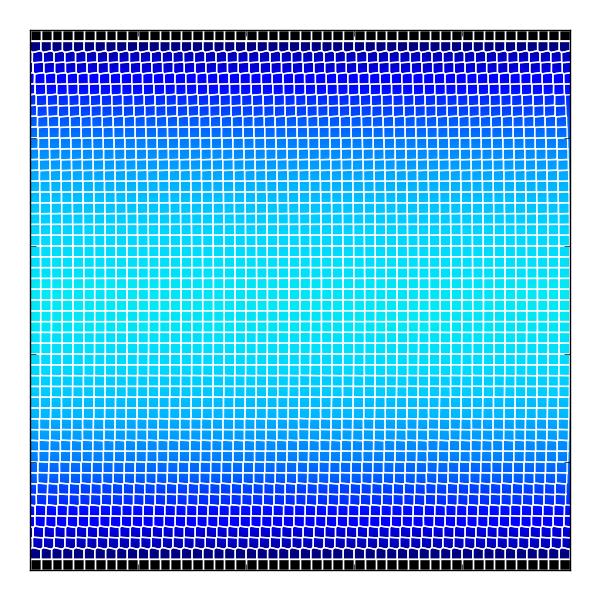
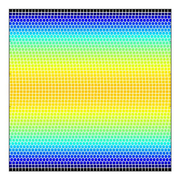
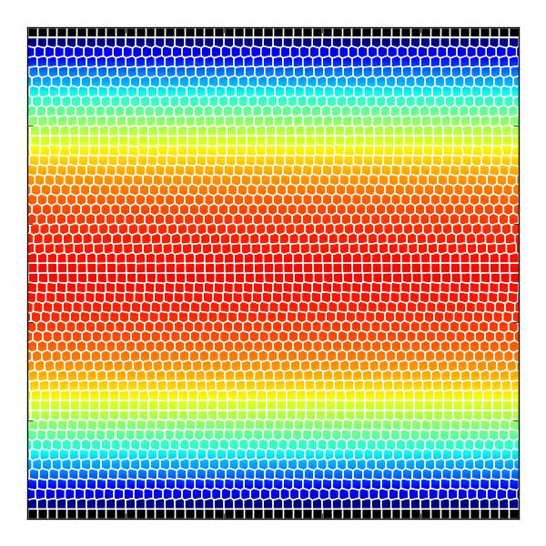
We run two different test problems. For the first one, both plates remain at rest and an external gradient of ${\rm d}p/{\rm d}x=-0.05$ is imposed. For the second test, the bottom plate is at rest and the upper plate moves at a constant speed of $U=0.1$. In both test simulations, the dynamic viscosity coefficient has been set to $\mu=0.05$. In Figure 8, we show the time evolution of the horizontal velocity profile both for the plane Poiseuille and Couette flows. In both cases, the numerical results match the analytic expectations very well. In Figures9 we also show maps of the velocity profile and the mesh geometry at different times for the Poiseuille case. The grid evolution shows how the Cartesian structure is progressively lost, but that the dynamic Voronoi mesh of AREPO successfully avoids any mesh-tangling effects.

4.4 Time-Dependent Circular Couette Flow

Figure 11: Geometry of the circular Couette flow. The left hand panel shows a schematic view of the two-dimensional problem. The right hand panel displays the actual initial mesh used in AREPO in a setup where we start the problem impulsively from rest. Each cylindrical boundary (at radii $R_{1}$ and $R_{2}$) is generated by two layers of cells, one side representing the solid cylinder and the other representing the fluid. These layers of cells are positioned along circles. The remainder of the fluid cells, originally at rest, are distributed like a Cartesian grid. The cells outside the outer cylinder are “auxiliary cells” and are only included to fill the computational domain, but do not exert any influence on the fluid inside the cylinders. The motion of the cylinders is prescribed to remain constant (with angular velocities $\Omega_{1}$ and $\Omega_{2}$), and thus represents a source of kinetic energy. The motion of the fluid in between the cylinders is induced by means of the no-slip boundary condition at the contact surface, and the momentum that is transported in the radial direction through the shear viscosity.

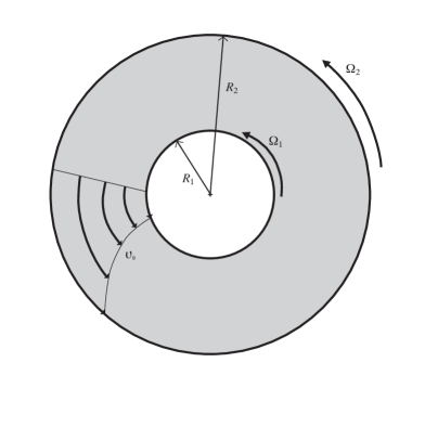
We now turn to a more challenging problem, which highlights the ability of our scheme to deal with geometrically complex boundary conditions. For purely azimuthal motion, the NS equations in the radial and tangential directions are

$$-\frac{v_{\theta}^{2}}{R} =-\frac{1}{\rho}\frac{{\rm d}P}{{\rm d}R}$$ (67a)

$$\rho\frac{\partial v_{\theta}}{\partial t} =\mu\frac{{\rm d}}{{\rm d}R}\left[\frac{1}{R}\frac{{\rm d}}{{\rm d}R}(Rv_{\theta})\right]~{}~{}.$$ (67b)

The exact solution of steady flow (i.e. $\partial v_{\theta}/\partial t=0$) between concentric cylinders with boundary conditions $v_{\theta}=\Omega_{1}R_{1}$ at $R=R_{1}$, and $v_{\theta}=\Omega_{2}R_{2}$ at $R=R_{2}$ is given by (e.g Kundu & Cohen, 2008)

$$v_{\theta,0}(R)=\frac{\frac{}{}\left(\Omega_{2}R_{2}^{2}-\Omega_{1}R_{1}^{2}\right)R^{2}-\left(\Omega_{2}-\Omega_{1}\right)R_{2}^{2}R_{1}^{2}}{R(R_{2}^{2}-R_{1}^{2})}~{}~{},$$ (68)

where $R_{i}$ and $\Omega_{i}$ ($i=1,2$) are the radii and angular velocities of the respective cylinders.

The impulsively-started version of this problem can be solved analytically by separation of variables (see Tranter, 1968; Graebel, 2007). The full solution can thus be written as $v_{\theta}(R,t)=v_{\theta,0}+\tilde{v}_{\theta}(R,t)$, where the time-dependent part has the form

$$\tilde{v}_{\theta}(R,t)=\sum\left\{C_{2}J_{1}(nR)+C_{2}Y_{1}(nR)\right\}e^{-\nu n^{2}t},$$

and $J_{1}$ and $Y_{1}$ are Bessel functions of the first and second kind, respectively. This time-dependent component is subject to the boundary conditions $\tilde{v}_{\theta}(R,t)=0$ at $R_{1}$ and $R_{2}$, thus allowing us to eliminate $C_{2}$:

$$\tilde{v}_{\theta}(R,t)=\sum_{s=1}^{\infty}\frac{A_{s}}{Y_{1}(n_{s}R_{1})}B_{1}(n_{s}R)e^{-\nu n_{s}^{2}t},$$

where the $n_{s}$ are the roots of the equation $B_{1}(nR)=0$ with $B_{1}(nR)\equiv J_{1}(nR)Y_{1}(nR_{1})-Y_{1}(nR)J_{1}(nR_{1})$.

Finally, the coefficients $A_{s}$ are determined by imposing the initial condition $\tilde{v}_{\theta}=-v_{\theta,0}$ at $t=0$. To solve for each coefficient independently, the steady state solution must be written in terms of a series expansion of $v_{\theta,0}$ in the basis functions $B_{1}(n_{s}R)$. After some algebraic manipulations, we obtain

$$\begin{split}v_{\theta,0}(R)=\pi\Omega_{2}R_{2}\sum_{s=1}^{\infty}&\frac{J_{1}(n_{s}R_{2})}{J_{1}^{2}(n_{s}R_{1})-J_{1}^{2}(n_{s}R_{2})}B_{1}(n_{s}R)\\ \times&\left[\cfrac{}{}J_{1}(n_{s}R_{1})-J_{1}(n_{s}R_{2})\frac{\Omega_{1}}{\Omega_{2}}\frac{R_{1}}{R_{2}}\right],\end{split}$$

and therefore the time-dependent component is given by

$$\begin{split}\tilde{v}_{\theta}(R,t)=-\frac{\pi}{R}\sum^{\infty}_{s=1}\frac{J_{1}(n_{s}R_{2})}{J_{1}^{2}(n_{s}R_{1})-J_{1}^{2}(n_{s}R_{2})}B_{1}(n_{s}R)e^{-\nu n_{s}^{2}t}\\ \times\left[\frac{}{}\Omega_{2}R_{2}J_{1}(n_{s}R_{1})-J_{1}(n_{s}R_{2})\Omega_{1}R_{1}\right]~{}~{}.\end{split}$$

Figure 12: A zoom showing the detailed mesh geometry around the inner boundary of the circular Couette flow, at two different times. The left hand panel shows a close-up view of the right panel of Fig. 11. The Voronoi faces that make up the cylindrical boundary are created by close pairs of points, which either lie inside the solid cylinder (red) or on the fluid side (black). The gray cells define the contact region of the fluid domain with the cylinder; here the no-slip boundary conditions are imposed. An analogous geometry applies for the outer cylinder. The panel on the right hand side shows the same region of the computational domain at a slightly later time, when the mesh filling the fluid region has started to react to the motion of the cylinder.

Collecting these results, the complete expression for the time-dependent angular velocity profile is

$$\begin{split}\Omega(R,t)=\frac{v_{\theta}}{R}-\frac{\pi}{R}\sum^{\infty}_{s=1}\frac{J_{1}(n_{s}R_{2})}{J_{1}^{2}(n_{s}R_{1})-J_{1}^{2}(n_{s}R_{2})}B_{1}(n_{s}R)e^{-\nu n_{s}^{2}t}\\ \times\left[\frac{}{}\Omega_{2}R_{2}J_{1}(n_{s}R_{1})-J_{1}(n_{s}R_{2})\Omega_{1}R_{1}\right]~{}~{}.\end{split}$$ (69)

We realize the moving boundary conditions in the present case through special Voronoi-cells with prescribed motion and boundary conditions, as described in Springel (2010). In the present case, we use two sets of mesh-generating points, each one consisting of a series of outside-inside pairs located on either side of the boundary and running parallel to it, so that two circular boundaries of radii $R_{1}$ and $R_{2}$ are defined which can be made to rotate at angular frequencies $\Omega_{1}$ and $\Omega_{2}$, respectively. Note that the only significant technical difference between this problem and the preceding examples is the way the boundary cells are prescribed to move; the rest of the numerical scheme remains unaltered.

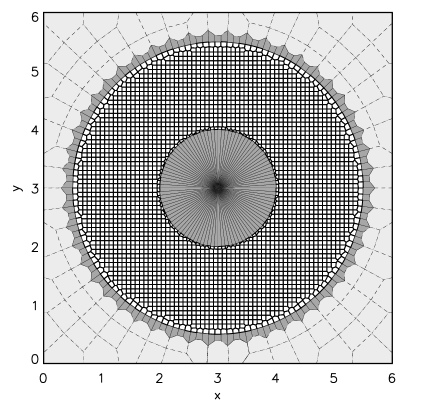
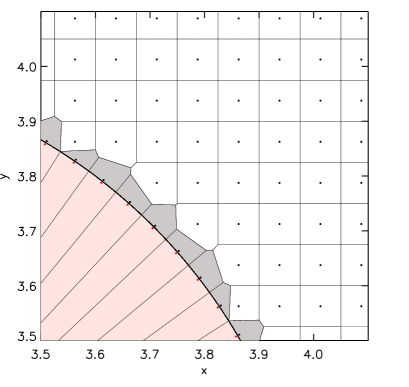
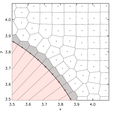
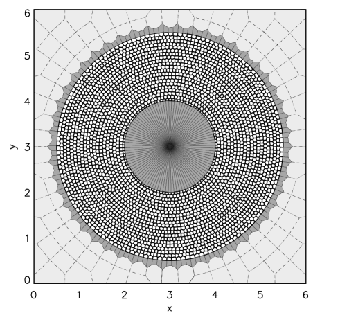
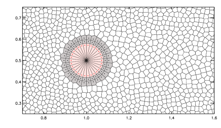
Figure 11 illustrates the geometry of the circular Couette flow, and our realization of a suitable mesh in AREPO. Since the equations of motion are always solved in the moving frame of the interfaces, there is no practical difference between stationary and moving boundaries when they are constructed as a part of the mesh. Figure 12 shows an enlargement of the mesh at the boundary corresponding to the inner cylinder, which is represented by a set of Voronoi faces that follow a circular path. Each one of these Voronoi faces is defined by two mesh generating points located on either side of the face, one of them outside the cylinder on the fluid side, the other inside the cylinder on the side that does not contain fluid. The right-hand panel of Fig. 12 shows the same region again, but at a slightly later time. This gives a sense of how the initial Cartesian mesh between the cylinders reacts to the fluid motion. Since the latter is azimuthal, the mesh eventually develops an axial geometry, independent of the initially Cartesian setup.

Our numerical experiment for this setup has the following parameters. The initial mesh as described in Figs. 11 and 12 contains 3,254 points, out of which 2,644 are regular fluid cells, 250 are boundary fluid cells, 250 are solid boundary cells and 110 are unused auxiliary cells that are only put in to fill up the total mesh area to an enclosing rectangular shape, as presently required by AREPO. The radial distance between the cylinders is spanned by 20 cells. The physical parameters of the Couette flow are $R_{1}=1$, $R_{2}=2.5$, $\Omega_{1}=0.5$, and $\Omega_{2}=0.1$, with a dynamic viscosity coefficient set to $\mu=0.005$. In addition, since the flow is started from rest, the pressure and density are taken to be uniform with values $\rho=P=1$. Figure 13 shows the time evolution of the angular velocity profile as it asymptotically converges to the steady state solution. The agreement of the numerical data points with the exact analytic solution (Eq. 69) is exceptional at all times.

Finally, we show in Fig. 14 the mesh geometry at the end of the calculation. Even though we have started the calculation with an initially Cartesian mesh, the memory of this geometry is lost during the calculation, and the mesh dynamically adapts to the azimuthal flow structure present in this problem. The transition from a Cartesian grid towards a cylindrical-like mesh can also be seen in the output sequence of the simulation shown in Fig. 13, where the values of the radial position of the cells start to segregate into a set of radial “bins”. The number of these radial clusters corresponds to the average number of cells along the radial direction.

Figure 13: Angular velocity profiles at different times for an impulsively started Taylor-Couette flow. For seven snapshots at times $t=0.5$, $20$, $40$, $60$, $80$, $100$, and $120$ we show the cell-centered values of $\Omega$, which are plotted as filled blue dots for all fluid cells in the calculation. No binning or averaging has been performed. The clustering of cell-center points as the system evolves is simply a consequence of the mesh adopting an axial symmetry in an adaptive fashion. The dashed lines give the time-dependent analytic solution of Eq. (69) at the corresponding times. The numerical results are almost indistinguishable from the exact solution. The red curve depicts the steady state solution to which the time-dependent solution eventually converges.

Figure 14: Mesh geometry for the circular Couette flow towards the end of the numerical integration. Even though we have started the calculation with an initially Cartesian mesh, this structure is quickly lost in favor of an on average azimuthal mesh geometry.

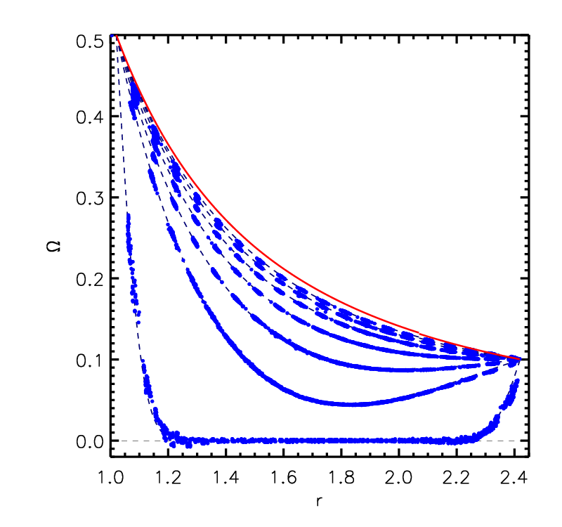
It is interesting to comment on the scatter of points – especially at the beginning of the simulation – as seen in the angular velocity profile of Figure 13. This is a reflection of the challenging initial mesh geometry. Although high-order schemes – fifth or sixth order – are not sensitive to the compliance of the mesh geometry with the flow, second order schemes are. In this particular case, an axially symmetric mesh geometry would be more suitable due to the characteristics of the flow. However, the main point of this test is to show how the mesh responds to the evolution of the problem, achieving rough axisymmetry despite the unfavorable initial setup.

As discussed by Springel (2010), our moving Voronoi mesh technique needs a “quality control” to keep cells sufficiently regular in order to avoid large errors in the spatial reconstruction. However, this modification of the mesh motion comes at a price: imagine a very strong compression along one direction (e.g. due to a very strong shock), then the mesh cells will acquire locally a high aspect ratio, which our mesh-quality control motions will try to eliminate, if needed by breaking the mesh symmetry (cell shapes are made “round” through small transverse motions). This is what happens when we start the Couette flow impulsively on a non-suitable mesh. The introduction of asymmetries in the mesh can influence the flow, in particular in situations where fluid instabilities develop (see the Kelvin Helmholtz instability test in Springel, 2010), where such asymmetric discretization errors can source growing perturbations. We note however that also on regular Cartesian meshes similar “grid-sourcing” errors exists. It appears unlikely that the poorer ability of the dynamic Voronoi mesh to maintain strict mesh symmetry is particularly detrimental for physical applications.

4.5 Flow Past a Circular Cylinder

Figure 15: Geometry of our wind tunnel set-up with a circular obstacle.

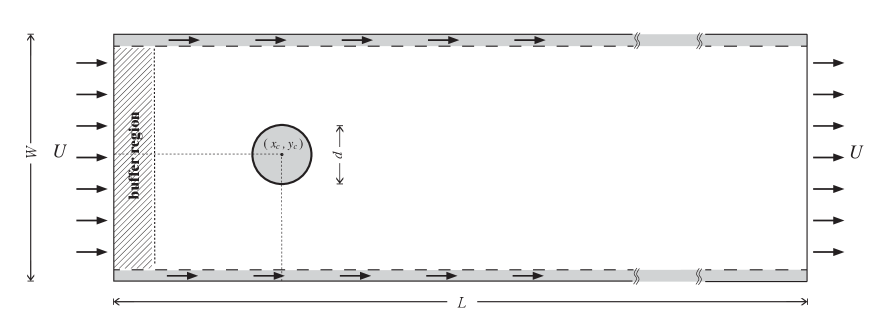
We next consider the flow over a circular cylinder immersed in a wind tunnel. The geometric setup of the problem is shown in Fig. 15. The flow comes from the left at a fixed horizontal velocity $U$. The upper and lower boundaries are also kept at constant velocity $U$. Far from the cylinder, at the right end of the computational domain, we impose again an exit velocity $U$. The injection and exit regions are forced to have the prescribed inflow and outflow mass fluxes at all times, something that we numerically impose through small “buffer” regions as labeled in Fig. 15. For static Cartesian grids, this buffer region does not need to extend more than one cell in the $x$-direction. However, moving grids require not only the injection of momentum from the left, but also the injection of new mesh-generating points, since the wind tunnel will otherwise produce a depletion of cells at the left end as the mesh generating points drift to the right in the direction of the flow. We address this issue by letting the mesh automatically generate new cells through cell splitting, as already implemented in AREPO (see examples in Springel, 2010). In doing this, some attention must however be paid to guarantee that the new cells reproduce the externally imposed inflow boundary conditions, which is most easily achieved with a sufficiently broad buffer region on the left end of the wind tunnel that covers the region where new cells are injected. Similarly, we employ the ability of AREPO to automatically remove mesh cells to prevent them from piling up on the right end of the wind tunnel. Altogether, we have created a wind tunnel that is filled with a mesh that blows with constant velocity from left to right, in a quasi-stationary state.

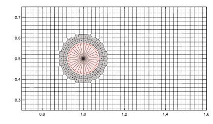
The other geometric parameters of the test problem we simulate here are the diameter $d$ of the cylindrical obstacle, the width $W$ of the tunnel and its length $L$. We have chosen $W=6.25\,d$ and $L=5\,W=31.25d\,$, and have scaled all length units such that $W=1.0$. The flexibility of the Voronoi mesh allows us to easily embed a cylindrical obstacle within the initially Cartesian background grid that fills the tunnel. Fig. 16 shows how we can tailor the mesh construction to reproduce the curved surface of the cylinder, using techniques similar to those that we used for the circular Couette flow problem.

The physical properties of the problem are primarily determined by the external velocity of the flow, $U$, and the dynamic viscosity of the fluid $\mu$. In our numerical experiments we set the external flow velocity to $U=0.5$, and combine this with constant initial pressure and density ($\rho=P=1$). We take the fluid to be described by an ideal gas equation of state with adiabatic index $\gamma=5/3$. The characteristic Reynolds number of the problem can then be defined by

$$Re=\frac{U\,d}{\nu}=\frac{U\,d\,\rho}{\mu}$$ (70)

where $\rho$ might however vary in time and space since the flow is fully compressible.

We have performed several numerical experiments of this problem using the viscous module added to AREPO. In each of these simulations, the Reynolds number is the only relevant quantity being changed. This is accomplished by changing $\mu$ exclusively, while keeping the other parameters fixed. Fig. 16 (upper panel) shows the initial setup for all the runs, which consist of a circular cylinder plus a Cartesian background grid of $250\times 50$ mesh generating points. The dynamic viscosity coefficient $\mu$ takes five different values: $2.5\times 10^{-2}$, $5\times 10^{-3}$, $2.5\times 10^{-3}$, $1.25\times 10^{-3}$ and $8.3\times 10^{-4}$. These values correspond to Reynolds numbers of 2, 10, 20, 40 and 60.

For each one of the tests, we show the resulting streamlines at time $t=9.9$ (or an equivalent dimensionless time of $\bar{t}=tU/d\approx 31.0$) in Fig. 17. Below $Re\sim 40$, the flow is steady and symmetric above and below the cylinder. As the Reynolds number increases, the size of the wake behind the cylinder grows. Although in this example the structure of the wake is poorly resolved, the increase in $Re$ is accompanied by an increase of vorticity confined within the wake.

Figure 16: Mesh near a circular cylinder inside a wind tunnel. The mesh contains both stationary mesh-generating points (defining the solid cylinder and two layers of cells used to create the cylindrical solid surface) and moving mesh-generating points (the remainder of the grid). The upper panel shows the initial setup, which highlights the cells representing the solid cylinder, and the two layers of fluid cells for which the equations of hydrodynamics are solved as in a standard stationary mesh. The total number of cells in the wind tunnel is $12,478$ (roughly $250\times 50$). The perimeter of the cylinder is outlined by 30 cells, and its diameter is equivalent to eight cells across. The Voronoi faces in between the red and grey cells define the boundary at which the no-slip condition is imposed. The lower panel shows the same region at a later time. Whereas one layer of mesh-generating points surrounding the cylinder has remained stationary, the rest of the background mesh has moved downstream and transformed to a generic unstructured Voronoi mesh as it moves along with the fluid.

(a) $Re=2$

(b) $Re=10$

(c) $Re=20$

(d) $Re=40$

(e) $Re=60$

Figure 17: Streamlines for compressible gas flow around a cylinder at five different Reynolds numbers, as labeled.

Figure 18: Density contrast of compressible flow past a cylinder at five different Reynolds numbers, corresponding to $Re=2$, $10$, $20$, $40$, $100$, from top to bottom. All five numerical experiments were computed with a static Cartesian mesh at moderately high resolution ($1000\times 250$), where the cell size is 1/32 of the cylinder’s diameter.

Above $Re\sim 40$, the wake behind the cylinder starts to become unstable. This can be clearly seen in the streamline pattern of the $Re=60$ panel. As the wake becomes unstable, the symmetry between the upper and lower portions of the domain is broken, at which point the flow becomes unsteady, such that the streamlines are no longer a valid representation of the Lagrangian trajectories of fluid parcels. This marks the onset of the von Karman vortex street, and the eventual transition to fully developed turbulence.

To further illustrate the flexibility of the mesh construction in AREPO, we can repeat this experiment with the mesh generating points set to remain static, thus recovering an Eulerian grid code. In addition, we increase the resolution by a factor of four to better resolve the wake behind the cylinder. In Fig. 18, we show the density contrast for five different Reynolds numbers. For stationary flow, the density distribution traces the streamline topology. At $Re=100$, we can appreciate how the fully developed von Karman vortex street looks for a compressible gas.

4.6 Three Dimensions: Taylor-Couette Flow

Circular Couette flow is a stable, special case of the more complex and richer three-dimensional Taylor-Couette flow (Taylor, 1923). Taylor found that when the angular velocity of the inner cylinder is increased above a certain threshold, Couette flow becomes unstable. After this transition, different states have been identified, the most famous of which is the Taylor vortex flow, characterized by axisymmetric toroidal vortices. The diversity of states for Taylor-Couette flow has been explored in the past, most notably by Coles (1965) and Andereck et al. (1986). The latter work lists up to 18 different flow regimes observed in flow between independently rotating cylinders. Its “Andereck diagram”, which explores the stability of the Taylor-Couette problem for a variety of Reynolds numbers, has become the standard benchmark for computational experiments of flow between rotating cylinders.

Figure 19: Vertical slice of the three-dimensional Voronoi tessellation in Taylor-Couette flow at the time Taylor vortices have developed. This same slice is used when visualizing the $v_{x}$,$v_{y}$ and $v_{z}$ fields (Fig. 20b and Fig. 21).

Although the computational and experimental study of three-dimensional Couette flow peaked during the 1980’s with the classical works of Andereck et al. (1986) and Marcus (1984a, b), in recent years it has regained popularity (e.g. Dong, 2007; Avila et al., 2008; Meseguer et al., 2009a, b) mainly driven by the experimental studies of magnetized and unmagnetized rotating flows of Ji et al. (2001, 2006) and Sisan et al. (2004), which have resulted in significant progress on the characterization of the magnetorotaional instability (MRI; Balbus & Hawley, 1998) in the laboratory.

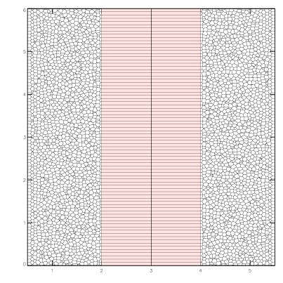
In this section, we briefly explore the evolution of Taylor-Couette flow on a moving Voronoi mesh. Although the AREPO code is not specifically designed for problems with symmetric geometries where static cylindrical meshes have proven to be more suitable, we have included this test to emphasize that our method works in three dimensions in an analogous way to the two-dimensional examples shown above. It is straightforward to extend the two-dimensional Couette flow shown above to three dimensions using AREPO. Since the mesh is obtained from a distribution of mesh-generating points, all that is needed is to replicate the initial conditions shown in Figure 13 in the vertical direction (about 80 times) to fill up a cubic box.

A standard validation for a Taylor-Couette simulation with azimuthal and axial periodicity may include, for example (Avila, private communication): obtaining perfect axial symmetry at low Reynolds number (i.e. circular Couette flow ), followed by obtaining the first bifurcation to axially symmetric Taylor vortices, and by reaching the second bifurcation to wavy vortices. These transitions occur sequentially as the angular velocity of the inner cylinder is increased while keeping the outer cylinder stationary (see the phase diagram of Andereck et al., 1986). However, it is not the purpose of this section to explore these transitions exhaustively; we only want to show that the third dimension works with our technique. We thus have focused on a particular configuration: counter-rotating Taylor-Couette flow, for which it is easy to obtain axially symmetric Taylor vortices (although these might relax back to Couette flow after several rotation periods; e.g. Liao et al., 1999). The geometry described in Fig. 11 is replicated in the vertical direction such that the computational domain is now a cube of dimensions $6\times 6\times 6$, with periodic boundary conditions in the $z$-direction. The initially Cartesian mesh will eventually relax in all directions as the flow evolves (Fig. 19). The cylinder is effectively infinite, like in the two-dimensional case, except that this time there is no imposed symmetry along the $z$-direction. We choose the cylinder radii to be $R_{1}=1.0$ and $R_{2}=2.5$, just like in the 2D example, and the respective angular velocities are $\Omega_{1}=0.8$ $\Omega_{2}=-0.5$ (counterrotating). The dynamic viscosity is $\mu=0.005$ and the fluid is started from rest with $\rho=P=1$. The inner and outer Reynolds numbers ($Re_{i}\equiv R_{i}\Omega_{i}(R_{2}-R_{1})\rho/\mu$; e.g. Liao et al., 1999) are $R_{1}=240$ and $R_{2}=-375$, respectively.

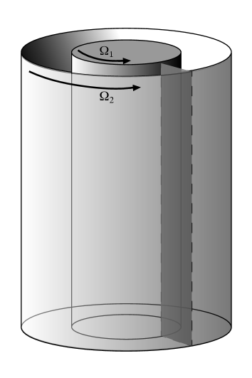
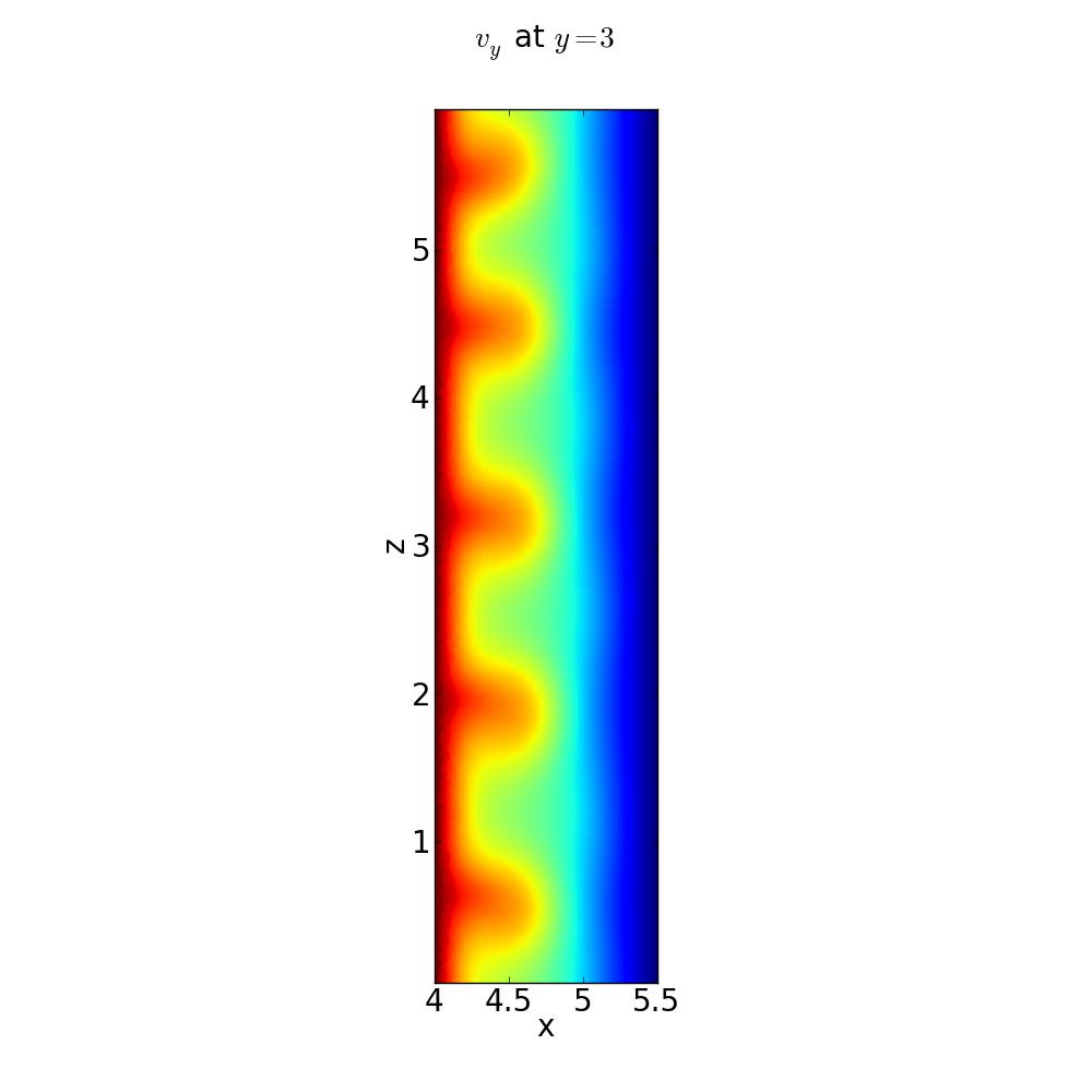
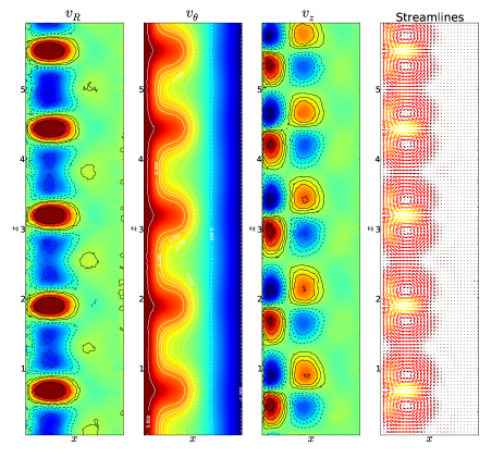
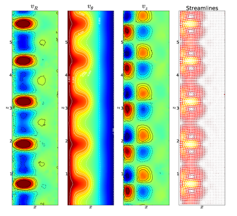
The geometry of the problem is shown in Fig. 20a. A vertical slice is taken at a time when the Taylor vortices have developed (the corresponding sliced mesh is shown in Fig. 19). The azimuthal velocity on that slice shows deviations from the symmetry in $z$ present in the circular Couette regime (Fig. 20b). Looking at the poloidal velocity field on that same slice ($v_{x}$ and $v_{z}$ in Fig. 21) one can appreciate, near the inner cylinder, the circular vertical motion characteristic of the Taylor vortices.

In Figure 21, we show the velocity field of this Taylor-Couette experiment at time $t=128$ for two different slices of the volume: (a) along the $x$-axis, and (b) along the $y$-axis (i.e. at $90^{\circ}$ from the first slice). Except for the numerical noise, the two solutions are nearly indistinguishable, evidence of a global axially symmetric Taylor vortex flow (for a very similar configuration, see Fig. 3 in Liao et al., 1999). This flow starts to develop at time $t\sim 60$ and remains essentially unaltered for several rotation periods. At much longer time scales, the flow would presumably decay back to a two-dimensional Couette flow as seen in the roughly similar test carried out by Liao et al. (1999).

Figure 20: a) Illustration of the three-dimensional flow between two independently rotating cylinders. The figure shows a plane along the radial direction where the local velocity field is evaluated. b) Velocity field in the $y$-direction between the cylinders for a slice defined by $y=3$ (i.e. along the diameter of both cylinders). For this particular plane, $v_{y}$ is equivalent to the azimuthal velocity $v_{\theta}$. The color scale goes from $v_{y}=\Omega_{2}R_{2}=-1.25$ (blue) to $v_{y}=\Omega_{1}R_{1}=0.8$ (red). This example shows that $v_{\theta}$ is no longer independent of $z$. Thus the two-dimensional solution of Eq. (69) is no longer valid.

Figure 21: Velocity structure of axisymmetric Taylor vortex flow at time $t=119$ at two different meridian planes separated by $90^{\circ}$. The poloidal velocity field ($v_{R},v_{z}$) is color mapped in the linear range [$-0.08$ (blue), $+0.08$ (red)], while the azimuthal field ($v_{\theta}$) is color mapped in the linear range [$-1.2$ (blue), $0.6$(red)]. The streamlines illustrate the vector field in the poloidal plane, showing with clarity the nature of Taylor vortices.

5 Concluding Remarks

We have presented a new numerical approach for solving the three-dimensional, compressible NS equations on a dynamic mesh using the new astrophysical code AREPO. This novel approach, an extension of the finite volume method, defines the computational mesh as a Voronoi tessellation moving with the local flow. The advantages of using a dynamic Voronoi mesh for transient and stationary flows under diverse boundary conditions has been addressed. The implicit adaptivity of the quasi-Lagrangian mesh elements, in addition to the well-behaved topological properties of the Voronoi tessellation, ensure both geometric flexibility and low numerical diffusivity. In addition, the shock capturing, second-order-accurate finite-volume scheme implemented in the rest-frame of each moving cell provides high accuracy.

We have described in detail the algorithm used to estimate the viscous diffusion of momentum across inter-cell boundaries. Our scheme produces smoothly varying estimates of the viscous terms, resulting in accurate and stable solutions. The method extends previously known finite-volume formulations of the NS equations with the introduction of a new reconstruction scheme that represents a compromise between the use of piece-wise constant gradients and fully consistent quadratic-reconstruction schemes.

For pure hydrodynamic flow, the CPU time consumption of our code per timestep is typically quite a bit higher than for structured mesh codes or SPH codes, for the same number of resolution elements. In three dimensions, the factor is close to $2$ relative to SPH (if 64 smoothing neighbors are used), and up to $\sim 3$ relative to a Cartesian mesh codes. The additional computational time goes mostly into the Voronoi mesh construction overhead, which is simply not needed by a structured mesh code, and also into an enlarged computational cost for the flux computations. The latter comes about because of a larger number of faces per cell (in 3D, there are 6 sides for a cubical cell, but for a 3D Voronoi mesh, we have of order $\sim 12$ sides for each polyhedral cell). It is however important to note that other, problem-dependent factors should be taken into account when assessing the performance in practice. For example, if large bulk velocities are present, our method can take considerably larger timesteps than a corresponding fixed mesh code. Also, because the advection errors are reduced in our scheme, fewer cells are required to reach a given accuracy, so that our code can then end up being computationally more efficient. We also note that once self-gravity is included (as in many of our primary target applications in astrophysics), the relative speed difference in the hydrodynamic part between the structured fixed mesh and our moving Voronoi mesh becomes much less of an issue, because the cost of calculating self-gravity sufficiently accurately for arbitrary geometries substantially reduces the relative importance of the hydrodynamical cost.

As part of our study, we have verified the reliability of our new method through a series of example calculations that range from simple flows with known analytic solutions to traditional experiments of well-known quantitative behavior. The demonstrated ability of the scheme to reproduce exact solutions as a function of time, even if the flow is started impulsively from rest, is reassuring. These examples also show the flexibility of the scheme in the presence of different solid surfaces moving in diverse ways. In all of these examples, the overall structure of the numerical scheme is identical, and the boundary conditions are set solely by the prescribed motion of the surfaces, which consist of controlled collections of Voronoi cells.

Although we have tested the performance of AREPO in configurations possessing a high degree of symmetry, it is in complex asymmetric problems where the moving-mesh approach would show all its power. The flexibility of the Lagrangian nature of the mesh will allow us to simulate, for example, complex astrophysical objects where viscosity is presumed to play a significant role. One such problem is the simulation of accretion disks around young stars. Although angular momentum transport in accretion disks is attributed to turbulence (most likely of magneto-hydrodynamic nature), this process is usually modeled both analytically (e.g. Shakura & Sunyaev, 1973; Lynden-Bell & Pringle, 1974; Pringle, 1981; Lin & Pringle, 1987) as well numerically (e.g. Kley & Lin, 1992; Masset, 2000; D’Angelo et al., 2002; de Val-Borro et al., 2006; Paardekooper & Mellema, 2006; Mudryk & Murray, 2009, just to name a few) by laminar flow in the presence of turbulent viscosity (Boussinesq approximation to eddy viscosity), due to the computational cost of global models of magneto-hydrodynamic disks. Another application of viscous flow is the plasma viscosity at galaxy cluster scales (e.g. Sijacki & Springel, 2006). However, it is likely that in such systems viscosity, as well as thermal conduction, is anisotropic (Braginskii, 1965; see Dong & Stone, 2009 for an example). In such a case, the viscous stress tensor in Eq. (6) can be easily generalized to include the up to seven independent viscosity coefficients (Lifshitz & Pitaevskii, 1981). It will be particularly exciting to couple the local anisotropy directly to the magnetic field topology, with the latter calculated self-consistently using a recent magnetohydrodynamics implemention in AREPO (Pakmor et al., 2011).

Its powerful flexibility will make AREPO an interesting code both for astrophysical simulations of viscous flow, but potentially also in engineering applications where the ability to cope with curved and moving boundaries is particularly attractive.

Appendix A Gradient Extrapolation Coefficients

The extrapolation of the velocity gradients (e.g. Eq. 40) requires a numerical estimate of the gradient matrix as well as an estimate for the time derivative of the gradient. For the latter, the tensors $A_{\alpha\beta b}$ and $B_{\alpha\beta ba}$ are needed (Eq. 38). Both tensors depend on the cell-centered scalar quantities as well as their gradients. The values of $A_{\alpha\beta b}$ are (e.g. Toro, 2009)

$$A_{\alpha\beta x}=A_{\alpha\beta 1}=\begin{pmatrix}v_{x}&\rho&0&0&0\\ 0&v_{x}&0&0&1/\rho\\ 0&0&v_{x}&0&0\\ 0&0&0&v_{x}&0\\ 0&\gamma P&0&0&v_{x}\\ \end{pmatrix},$$ (71)

$$A_{\alpha\beta y}=A_{\alpha\beta 2}=\begin{pmatrix}v_{y}&0&\rho&0&0\\ 0&v_{y}&0&0&0\\ 0&0&v_{y}&0&1/\rho\\ 0&0&0&v_{y}&0\\ 0&0&\gamma P&0&v_{y}\\ \end{pmatrix},$$ (72)

$$A_{\alpha\beta z}=A_{\alpha\beta 3}=\begin{pmatrix}v_{z}&0&0&\rho&0\\ 0&v_{z}&0&0&0\\ 0&0&v_{z}&0&0\\ 0&0&0&v_{z}&1/\rho\\ 0&0&0&\gamma P&v_{z}\\ \end{pmatrix}.$$ (73)

The tensor $B_{\alpha\beta ba}\equiv\partial_{a}A_{\alpha\beta b}=A_{\alpha\beta b,a}$ (with $a,b=x,y,z\;\text{or }1,2,3$ and $\alpha,\beta=0,1,2,3,4$) has components:

$$B_{\alpha 0xa} =\begin{pmatrix}\partial_{x}v_{x}&\partial_{y}v_{x}&\partial_{z}v_{x}\\ 0&0&0\\ 0&0&0\\ 0&0&0\\ 0&0&0\\ \end{pmatrix}~{}~{},$$ (74)

$$B_{\alpha 0ya} =\begin{pmatrix}\partial_{x}v_{y}&\partial_{y}v_{y}&\partial_{z}v_{y}\\ 0&0&0\\ 0&0&0\\ 0&0&0\\ 0&0&0\\ \end{pmatrix}~{}~{},$$ (75)

$$B_{\alpha 0za} =\begin{pmatrix}\partial_{x}v_{z}&\partial_{y}v_{z}&\partial_{z}v_{z}\\ 0&0&0\\ 0&0&0\\ 0&0&0\\ 0&0&0\\ \end{pmatrix}~{}~{},$$ (76)

$$B_{\alpha 1xa} =\begin{pmatrix}\partial_{x}\rho&\partial_{y}\rho&\partial_{z}\rho\\ \partial_{x}v_{x}&\partial_{y}v_{x}&\partial_{z}v_{x}\\ 0&0&0\\ 0&0&0\\ \gamma\partial_{x}P&\gamma\partial_{y}P&\gamma\partial_{z}P\\ \end{pmatrix}~{}~{},$$ (77)

$$B_{\alpha 1ya} =\begin{pmatrix}0&0&0\\ \partial_{x}v_{y}&\partial_{y}v_{y}&\partial_{z}v_{y}\\ 0&0&0\\ 0&0&0\\ 0&0&0\\ \end{pmatrix}~{}~{},$$ (78)

$$B_{\alpha 1za} =\begin{pmatrix}0&0&0\\ \partial_{x}v_{z}&\partial_{y}v_{z}&\partial_{z}v_{z}\\ 0&0&0\\ 0&0&0\\ 0&0&0\\ \end{pmatrix}~{}~{},$$ (79)

$$B_{\alpha 2xa} =\begin{pmatrix}0&0&0\\ 0&0&0\\ \partial_{x}v_{x}&\partial_{y}v_{x}&\partial_{z}v_{x}\\ 0&0&0\\ 0&0&0\\ \end{pmatrix}~{}~{},$$ (80)

$$B_{\alpha 2ya} =\begin{pmatrix}\partial_{x}\rho&\partial_{y}\rho&\partial_{z}\rho\\ 0&0&0\\ \partial_{x}v_{y}&\partial_{y}v_{y}&\partial_{z}v_{y}\\ 0&0&0\\ \gamma\partial_{x}P&\gamma\partial_{y}P&\gamma\partial_{z}P\\ \end{pmatrix}~{}~{},$$ (81)

$$B_{\alpha 2za} =\begin{pmatrix}0&0&0\\ 0&0&0\\ \partial_{x}v_{z}&\partial_{y}v_{z}&\partial_{z}v_{z}\\ 0&0&0\\ 0&0&0\\ \end{pmatrix}~{}~{},$$ (82)

$$B_{\alpha 3xa} =\begin{pmatrix}0&0&0\\ 0&0&0\\ 0&0&0\\ \partial_{x}v_{x}&\partial_{y}v_{x}&\partial_{z}v_{x}\\ 0&0&0\\ \end{pmatrix}~{}~{},$$ (83)

$$B_{\alpha 3ya} =\begin{pmatrix}0&0&0\\ 0&0&0\\ 0&0&0\\ \partial_{x}v_{y}&\partial_{y}v_{y}&\partial_{z}v_{y}\\ 0&0&0\\ \end{pmatrix}~{}~{},$$ (84)

$$B_{\alpha 3za} =\begin{pmatrix}\partial_{x}\rho&\partial_{y}\rho&\partial_{z}\rho\\ 0&0&0\\ 0&0&0\\ \partial_{x}v_{z}&\partial_{y}v_{z}&\partial_{z}v_{z}\\ \gamma\partial_{x}P&\gamma\partial_{y}P&\gamma\partial_{z}P\\ \end{pmatrix}~{}~{},$$ (85)

$$B_{\alpha 4xa} =\begin{pmatrix}0&0&0\\ -\cfrac{\partial_{x}\rho}{\rho^{2}}&-\cfrac{\partial_{y}\rho}{\rho^{2}}&-\cfrac{\partial_{z}\rho}{\rho^{2}}\\ 0&0&0\\ 0&0&0\\ \partial_{x}v_{x}&\partial_{y}v_{x}&\partial_{z}v_{x}\\ \end{pmatrix}~{}~{},$$ (86)

$$B_{\alpha 4ya} =\begin{pmatrix}0&0&0\\ 0&0&0\\ -\cfrac{\partial_{x}\rho}{\rho^{2}}&-\cfrac{\partial_{y}\rho}{\rho^{2}}&-\cfrac{\partial_{z}\rho}{\rho^{2}}\\ 0&0&0\\ \partial_{x}v_{y}&\partial_{y}v_{y}&\partial_{z}v_{y}\\ \end{pmatrix}~{}~{},$$ (87)

$$B_{\alpha 4za} =\begin{pmatrix}0&0&0\\ 0&0&0\\ 0&0&0\\ -\cfrac{\partial_{x}\rho}{\rho^{2}}&-\cfrac{\partial_{y}\rho}{\rho^{2}}&-\cfrac{\partial_{z}\rho}{\rho^{2}}\\ \partial_{x}v_{z}&\partial_{y}v_{z}&\partial_{z}v_{z}\\ \end{pmatrix}~{}~{}.$$ (88)

References

- Andereck et al. (1986) Andereck C. D., Liu S. S., Swinney H. L., 1986, Journal of Fluid Mechanics, 164, 155
- Ata et al. (2009) Ata R., Soula mani A., Chinesta F., 2009, International Journal for Numerical Methods in Fluids, 59, 19
- Avila et al. (2008) Avila M., Belisle M. J., Lopez J. M., Marques F., Saric W. S., 2008, Journal of Fluid Mechanics, 601, 381
- Balbus & Hawley (1998) Balbus S. A., Hawley J. F., 1998, Reviews of Modern Physics, 70, 1
- Barth (1992) Barth T. J., 1992, in AGARD, Special Course on Unstructured Grid Methods for Advection Dominated Flows. ed. C. Johnson
- Bauer & Springel (2011) Bauer A., Springel V., 2011, ArXiv e-prints
- Borgers & Peskin (1987) Borgers C., Peskin C. S., 1987, Journal of Computational Physics, 70, 397
- Brackbill & Monaghan (1988) Brackbill J., Monaghan J., 1988, Particle Methods in Fluid Dynamics and Plasma Physics (Computer Physics Communications, Vol. 48). Amsterdam: North-Holland
- Braginskii (1965) Braginskii S. I., 1965, Reviews of Plasma Physics, 1, 205
- Christov (2009) Christov I., 2009, in Hyperbolic Problems: Theory, Numerics and Applications. Proceedings of Symposia in Applied Mathematics. Volume 67. ed. E. Tadmor, J.-G. Liu, A. E. Tzavaras
- Coirier (1994) Coirier W. J., 1994, PhD thesis, University of Michigan
- Coirier & Powell (1996) Coirier W. J., Powell K. G., 1996, AIAA Journal, 34, 938
- Colella & Woodward (1984) Colella P., Woodward P. R., 1984, Journal of Computational Physics, 54, 174
- Coles (1965) Coles D., 1965, Journal of Fluid Mechanics, 21, 385
- D’Angelo et al. (2002) D’Angelo G., Henning T., Kley W., 2002, A&A, 385, 647
- de Val-Borro et al. (2006) de Val-Borro M., Edgar R. G., Artymowicz et al., 2006, MNRAS, 370, 529
- Dong & Stone (2009) Dong R., Stone J. M., 2009, ApJ, 704, 1309
- Dong (2007) Dong S., 2007, Journal of Fluid Mechanics, 587, 373
- Duffell & MacFadyen (2011) Duffell P. C., MacFadyen A. I., 2011, ArXiv e-prints
- Dukowicz et al. (1989) Dukowicz J. K., Cline M. C., Addessio F. L., 1989, Journal of Computational Physics, 82, 29
- Frink (1994) Frink N. T., 1994, AIAA Tech. Rep.
- Graebel (2007) Graebel W. P., 2007, Advanced fluid mechanics. Academic Press, Elsevier
- Hirt et al. (1974) Hirt C. W., Amsden A. A., Cook J. L., 1974, Journal of Computational Physics, 14, 227
- Ji et al. (2006) Ji H., Burin M., Schartman E., Goodman J., 2006, Nature, 444, 343
- Ji et al. (2001) Ji H., Goodman J., Kageyama A., 2001, MNRAS, 325, L1
- Kley & Lin (1992) Kley W., Lin D. N. C., 1992, ApJ, 397, 600
- Kundu & Cohen (2008) Kundu P. K., Cohen I. M., 2008, Fluid Mechanics: Fourth Edition. London: Academic Press, Elsevier
- Landau & Lifshitz (1959) Landau L. D., Lifshitz E. M., 1959, Fluid mechanics. Oxford: Pergamon Press
- LeVeque (2002) LeVeque R. J., 2002, Finite Volume Methods for Hyperbolic Problems. Cambridge University Press. Cambridge, UK: Cambridge University Press
- Liao et al. (1999) Liao C. B., Jane S. J., Young D. L., 1999, International Journal for Numerical Methods in Fluids, 29, 827
- Lifshitz & Pitaevskii (1981) Lifshitz E. M., Pitaevskii L. P., 1981, Physical kinetics. Oxford: Pergamon Press, 1981
- Lin & Pringle (1987) Lin D. N. C., Pringle J. E., 1987, MNRAS, 225, 607
- Loh (2007) Loh C. Y., 2007, in Cure of Pathological Behaviors, AIAA Paper, pp. 2007–4463
- Lynden-Bell & Pringle (1974) Lynden-Bell D., Pringle J. E., 1974, MNRAS, 168, 603
- MacCormack & Baldwin (1975) MacCormack R. W., Baldwin B. S., 1975, AIAA, Aerospace Sciences Meeting
- March (2002) March N. H. andTosi M. P., 2002, Introduction to Liquid State Physics. World Scientific Publishing Company
- Marcus (1984a) Marcus P. S., 1984a, Journal of Fluid Mechanics, 146, 45
- Marcus (1984b) —, 1984b, Journal of Fluid Mechanics, 146, 65
- Masset (2000) Masset F., 2000, A&As, 141, 165
- Mavriplis (1997) Mavriplis D. J., 1997, Annual Review of Fluid Mechanics, 29, 473
- Mavriplis & Jameson (1990) Mavriplis D. J., Jameson A., 1990, AIAA Journal, 28, 1415
- Meier et al. (2005) Meier K., Laesecke A., Kabelac S., 2005, J. Chem. Phys., 122, 014513
- Meseguer et al. (2009a) Meseguer A., Mellibovsky F., Avila M., Marques F., 2009a, Phys. Rev. E, 79, 036309
- Meseguer et al. (2009b) —, 2009b, Phys. Rev. E, 80, 046315
- Mishev (1998) Mishev I. D., 1998, Numerical Methods for Partial Differential Equations, 14, 193
- Mudryk & Murray (2009) Mudryk L. R., Murray N. W., 2009, New Ast., 14, 71
- Munikrishna (2009) Munikrishna N., 2009, PhD thesis, Indian Institute of Science
- Norris et al. (2010) Norris S. E., Were C. J., Richards P. J., Mallinson G. D., 2010, International Journal for Numerical Methods in Fluids
- Paardekooper & Mellema (2006) Paardekooper S.-J., Mellema G., 2006, A&A, 450, 1203
- Pakmor et al. (2011) Pakmor R., Bauer A., Springel V., 2011, MNRAS, 418, 1392
- Price (2012) Price D. J., 2012, MNRAS, 420, L33
- Pringle (1981) Pringle J. E., 1981, ARA&A, 19, 137
- Puigt et al. (2010) Puigt G., Auffray V., Müller J., 2010, Journal of Computational Physics, 229, 1425
- Robertson et al. (2010) Robertson B. E., Kravtsov A. V., Gnedin N. Y., Abel T., Rudd D. H., 2010, MNRAS, 401, 2463
- Ruszkowski et al. (2004) Ruszkowski M., Brüggen M., Begelman M. C., 2004, ApJ, 615, 675
- Serrano & Español (2001) Serrano M., Español P., 2001, Phys. Rev. E, 64, 046115
- Shakura & Sunyaev (1973) Shakura N. I., Sunyaev R. A., 1973, A&A, 24, 337
- Sijacki & Springel (2006) Sijacki D., Springel V., 2006, MNRAS, 371, 1025
- Sisan et al. (2004) Sisan D. R., Mujica N., Tillotson W. A., Huang Y.-M., Dorland W., Hassam A. B., Antonsen T. M., Lathrop D. P., 2004, Physical Review Letters, 93, 114502
- Springel (2010) Springel V., 2010, MNRAS, 401, 791
- Sukumar (2009) Sukumar N., 2009, International Journal for Numerical Methods in Engineering, 57, 1
- Sukumar & Bolander (2009) Sukumar N., Bolander J. E., 2009, in Tessellations in the Sciences: Virtues, Techniques and Applications of Geometric Tilings.
- Sukumar et al. (1998) Sukumar N., Moran B., Belytschko T., 1998, International Journal for Numerical Methods in Engineering, 43, 839
- Taylor (1923) Taylor G. I., 1923, Royal Society of London Philosophical Transactions Series A, 223, 289
- Toro (2009) Toro E. F., 2009, Riemann solvers and numerical methods for fluid dynamics. A practical introduction. 3rd Edition. Springer
- Tranter (1968) Tranter C. J., 1968, Bessel Functions with Some Physical Applications. London: English University Press, London
- Venkatakrishnan (1996) Venkatakrishnan V., 1996, AIAA Journal, 34, 533
- Vogelsberger et al. (2011) Vogelsberger M., Sijacki D., Keres D., Springel V., Hernquist L., 2011, ArXiv e-prints