3D Solar Null Point Reconnection MHD Simulations

Abstract

Numerical MHD simulations of 3D reconnection events in the solar corona have improved enormously over the last few years, not only in resolution, but also in their complexity, enabling more and more realistic modeling. Various ways to obtain the initial magnetic field, different forms of solar atmospheric models as well as diverse driving speeds and patterns have been employed. This study considers differences between simulations with stratified and non-stratified solar atmospheres, addresses the influence of the driving speed on the plasma flow and energetics, and provides quantitative formulas for mapping electric fields and dissipation levels obtained in numerical simulations to the corresponding solar quantities. The simulations start out from a potential magnetic field containing a null-point, obtained from a Solar and Heliospheric Observatory (SOHO) magnetogram extrapolation approximately 8 hours before a C-class flare was observed. The magnetic field is stressed with a boundary motion pattern similar to — although simpler than — horizontal motions observed by SOHO during the period preceding the flare. The general behavior is nearly independent of the driving speed, and is also very similar in stratified and non-stratified models, provided only that the boundary motions are slow enough. The boundary motions cause a build-up of current sheets, mainly in the fan-plane of the magnetic null-point, but do not result in a flare-like energy release. The additional free energy required for the flare could have been partly present in non-potential form in the initial state, with subsequent additions from magnetic flux emergence or from components of the boundary motion that were not represented by the idealized driving pattern.

1 Introduction

sec:introduction There have been different attempts to initialize the magnetic field of the photosphere and corona for numerical simulations; amongst others by elimination of the complex observed small scale structure by the use of several photospheric magnetic monopole sources (Priest, Bungey, and Titov, 1997), by flux emergence experiments (Archontis et al., 2004), as well as by extrapolation (e.g. Masson et al., 2009) of solar observatory magnetograms, e.g. from SOHO. The latter type has typically been used together with potential extrapolations, for simplicity reasons as well as due to the limited availability of vector magnetograms. As potential magnetic fields contain no free magnetic energy, these cannot directly be used for explaining how flare events take place and where the released energy arises from. Therefore, to use a potential magnetic field as the basis for an investigation of a flare event, the field must be stressed into a state where it contains sufficient free magnetic energy to account for the energy release event. There are different ways by which this may be accomplished. A simple approach is to impose boundary motions that resemble the ones derived from observations (Bingert and Peter, 2011; Gudiksen and Nordlund, 2002). An alternative, more challenging approach is to stress the system by allowing additional magnetic flux to enter through photospheric magnetic flux emergence (Fan and Gibson, 2003). In the solar context both of these processes take place simultaneously, while experiments typically concentrate on a single type of stressing, in order to investigate in detail its influence on the dynamical evolution of the magnetic field.

The present investigation is an extension of the work done by Masson et al. (2009). They studied the evolution preceding a specific flare event observed with SOHO, starting by taking a magnetogram from about 8 hours before the flare and deriving a potential magnetic field. Due to the presence of a ‘parasitic’ magnetic polarity, the resulting magnetic field contains a magnetic null-point. From the motions of observed magnetic fragments a schematic photospheric velocity flow was constructed, and was used to stress this initially potential magnetic field. The imposed stress distorts the magnetic field, causing electric currents to build up in the vicinity of the magnetic null-point. The magnetic dissipation associated with the electric current allows a continuous reconnection to take place. The boundary driving together with the reconnection causes the null-point to move. The locations of the magnetic dissipation agree qualitatively with the locations of flare emission in various wavelength bands, which may be seen as evidence supporting a close association between reconnection at the magnetic null-point and the observed C-class flare.

The Masson et al. (2009) paper raises many interesting questions, some of which we attempt to answer in the present paper. We therefore let the same observations provide the basis for deriving a potential initial magnetic field, and employ the same imposed boundary stressing of the magnetic field, using the setup to investigate the impact of varying the amplitude of the driving speed, as well as the impact of allowing the experiment to take place in a gravitationally stratified setting.

The paper is organized as follows: In Section sec:methods we list the equations we solve, and briefly describe the numerical methods used to solve them. In Section sec:simulations we give an overview of the different numerical experiments, in Section sec:results we present and discuss the results, and finally in Section sec:conclusions we summarize the main results and conclusions.

2 Methods

sec:methods The simulations have been performed using the fully 3D resistive and compressible Stagger MHD code (Nordlund and Galsgaard, 1997a; Kritsuk et al., 2011). The following form of the resistive MHD equations are solved in the code:

$$\frac{\partial\rho}{\partial t} = -\nabla\cdot(\rho\mathbf{u})$$ (1)

$$\frac{\partial(\rho\mathbf{u})}{\partial t} = -\nabla\cdot(\rho\mathbf{u}\mathbf{u}+\underline{\underline{\tau}})-\nabla p$$ (2)

$$+\mathbf{j}\times\mathbf{B}+\rho\mathbf{g}$$

$$\frac{\partial e}{\partial t} = -\nabla\cdot(e\mathbf{u}+\mathbf{f_{e}})-p\nabla\cdot\mathbf{u}$$ (3)

$$+Q_{J}+Q_{\nu}$$

$$\frac{\partial\mathbf{B}}{\partial t} = -\nabla\times\mathbf{E}$$ (4)

$$\mathbf{j} = \nabla\times\mathbf{B}$$ (5)

$$\mathbf{E} = -\mathbf{u}\times\mathbf{B}+\eta\mathbf{j}$$ (6)

$$Q_{J} = \eta j^{2}$$ (7)

$$\nabla\cdot\mathbf{B} = 0$$ (8)

$$p = (\gamma-1)e$$ (9)

$$\tau_{ij} = -\nu_{ij}\rho S_{ij}$$ (10)

$$S_{ij} = \frac{1}{2}\left(\frac{\partial u_{i}}{\partial x_{j}}+\frac{\partial u_{j}}{\partial x_{i}}\right)$$ (11)

$$Q_{\nu} = \rho\sum_{ij}\nu_{ij}S_{ij}^{2}$$ (12)

$$\mathbf{f_{e}} = -\nu_{e}\rho\nabla(e/\rho)$$ (13)

where $\rho$ is the mass density, $\mathbf{u}$ the bulk velocity, $p$ the pressure, $\mathbf{j}$ the current density, $\mathbf{B}$ the magnetic field, $g$ the acceleration of gravity, $e$ the thermal energy per unit volume and $\eta$ the resistivity. $S_{ij}$ is the shear tensor, $\tau_{ij}$ the viscous stress tensor and $\mathbf{f_{e}}$ is a weak diffusive flux of thermal energy needed for numerical stability. The term $Q_{v}$ represents viscous dissipation, turning kinetic energy into heat, while $Q_{J}$ is the Joule dissipation, responsible for converting magnetic energy into heat.

The solution to the MHD equations is advanced in time using an explicit 3rd order predictor-corrector procedure (Hyman, 1979).

The version of the Stagger MHD code used here assumes an ideal gas law and includes no radiative cooling and heat conduction. The variables are located on different staggered grids, which allows for conservation of various quantities to machine precision. The staggering of variables has been chosen so $\nabla\cdot\mathbf{B}$ is among the quantities conserved to machine precision. Interpolation of variables between different staggered grids is handled by using 5th order interpolation. In a similar way spatial derivatives are computed using expressions accurate to 6th order. To minimize the influence of numerical diffusion dedicated operators are used for calculating both viscosity and resistivity. The viscosity is given by

$$\ilabel{eq:nu}\nu=\Delta d\left(\nu_{1}c_{f}+\nu_{2}|\mathbf{u}|+\nu_{3}\Delta d\;|-\nabla\cdot\mathbf{u}|_{+}\right),$$ (14)

where $\Delta d$ is the mesh size and $\nu_{1}=0.005-0.02$, $\nu_{2}=0.005-0.02$, and $\nu_{3}=0.2-0.4$ are dimensionless coefficients that provide a suitable amount of dissipation of fast mode waves ($\nu_{1}$), advective motions ($\nu_{2}$), and shocks ($\nu_{3}$). The expression $|-\nabla\cdot\mathbf{u}|_{+}$ denotes the positive part of the rate of compression $-\nabla\cdot\mathbf{u}$. $c_{f}$ is the fast mode speed defined by $c_{f}=\sqrt{(B^{2}+\gamma p)/\rho}$.

The resulting grid Reynolds numbers, $\Delta d\,c_{f}/\nu$, are on the order of 50 – 200 in regions with smooth variations, while in the neighborhood of shocks they are of the order of a few. The corresponding expression for the resistivity is

$$\ilabel{eq:eta}\eta=\Delta d\left(\nu_{1}c_{f}+\nu_{2}|\mathbf{u}|+\nu_{3}\Delta d\,|-\nabla\cdot\mathbf{u}_{\perp}|_{+}\right),$$ (15)

where $\mathbf{u}_{\perp}$ is the component of the velocity perpendicular to $\mathbf{B}$, and where the expression scaled by $\nu_{3}$ prevents electric current sheets from becoming numerically unresolved. The resulting magnetic grid Reynolds numbers are of the order of a few in current sheets, as required to keep such structures marginally resolved.

The overall scaling with $\Delta d$ ensures that advection patterns, waves, shocks and current sheets remain resolved by a few grids, independent of the mesh size.

The advantage of these three-part expressions for the viscosity and the resistivity, compared to having constant viscosity and resistivity is that constant values would have to be chosen on the order of the largest of these three term, in order to handle shocks and current sheets. In the rest of the volume the viscosity and resistivity would then be orders of magnitude larger than needed. As demonstrated in (Kritsuk et al., 2011) the results are quite similar to state of the art codes that use local Riemann solvers. Such codes also have dissipative behavior on the scale of individual cells – no numerical code is ’ideal’ in the sense that it presents solutions corresponding to zero resistivity.

In this article we refer to the $-\mathbf{u}\times\textbf{B}$ term in the induction equation as the advective electric field, while its counterpart $\eta\textbf{j}$ is referred to as the diffusive electric field.

3 Simulations

sec:simulations The experimental setup is inspired by the work by Masson et al. (2009). Our study sets out from a Fast Fourier Transform potential extrapolation applied to a level 1.8 SOHO/Michelson Doppler Imager magnetogram (Scherrer et al., 1995) from November 16, 2002 at 06:27 UT, 8 hour prior to a C-class flare occurrence in the AR10191 active region. The extrapolation leads to a 3D magnetic null-point topology with a clear fan and spine structure (Green, 1989; Priest and Titov, 1996). In order to allow periodic boundary conditions in the potential field extrapolation we applied a windowing function to the SOHO cutout of the active region AR10191, which decreases the field close to the boundary towards zero. This cutout from the complete solar disk SOHO data differs slightly from the one used by Masson et al. (2009). As a result, in our case the null-point is initially located at a height of about 4 Mm above the magnetogram, while in their case the null-point is located at a height of only 1.5 Mm above the magnetogram. The change in null position places our null-point in the corona proper and allows us to perform affordable simulations with stratified atmospheres, while at the same time it does not influence the nature of the current sheet formation, and still successfully describes a typical solar-like magnetic field geometry.

Numerically, a magnetic field derived from a potential extrapolation is not necessarily divergence free, and we therefore initially apply a divergence cleaning procedure, which removes the divergence (as measured by our specific numerical stretched mesh derivative operators) by iteratively applying a correction obtained from solving the Poisson equation

$$\ilabel{eq:divb}\Delta\delta\Phi=-\nabla\cdot\mathbf{B}.$$ (16)

The structure of the resulting initial magnetic field is illustrated in Figure fig:init_MHD.epsa and fig:init_MHD.epsb, showing a strong overall magnetic field and a weaker fan-spine structure close to the photospheric boundary, which is separately illustrated in Figure fig:spine_fan_zoom.eps. Note, that the field lines of the fan-spine topology were selected specifically to show the topology, and that the density of the field lines is therefore not representative of the magnetic flux density.

We performed two types of simulation; one type in which we imposed a 1-D gravitationally stratified atmosphere profile, and a second type with constant density and temperature. The density and temperature profiles are shown in Figure fig:density_compare.ps, and a summary of the simulation runs may be found in Table tab:simulations.

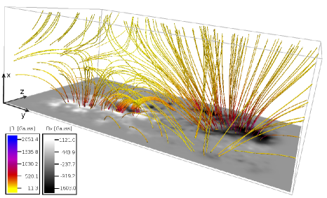
(a)

(b)

Figure 1.: Magnetic field resulting from the FFT extrapolation of the SOHO magnetogram taken on November 16, 2002. The region shown here is the entire computational box, having an extent of $60\times 175\times 100$ Mm. The slice represents the vertical component of the magnetic field. Black is the negative polarity, white is positive.fig:init˙MHD.eps

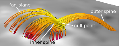
Figure 2.: Zoom in of Figure fig:init_MHD.eps (upper drawing) to the fan-spine topology, excluding the large scale field. The volume below the fan-plane is referred to as ‘the dome’.fig:spine˙fan˙zoom.eps

The magnetic fields are in all cases anchored at the vertical boundaries, which due to boundary conditions also prevent plasma from flowing in and out. The exception to this is run 1O, in which instead constant pressure is assumed at the lower boundary, and plasma flows through the boundary are allowed. Only minor differences were found between the open and closed boundary cases.

Figure 3.: Mass densities are presented in black, temperatures in gray. The solid line shows the 1D mass density and temperature profiles as a function of height $x$ [Mm] of all stratified runs. The dashed line illustrates the constant mass density and temperature of run 1, run 1O, run 2 run 3 and run 4.fig:density˙compare.ps

Run	boundary	max. driving [km s-1]	density [cm-3]	temperature [K]
1	closed	3.33	6.8$\times 10^{12}$	5.0$\times 10^{5}$
1O	open	3.33	6.8$\times 10^{12}$	5.0$\times 10^{5}$
2	closed	6.67	6.8$\times 10^{12}$	5.0$\times 10^{5}$
3	closed	10	6.8$\times 10^{12}$	5.0$\times 10^{5}$
4	closed	20	6.8$\times 10^{12}$	5.0$\times 10^{5}$
1S	closed	3.33	[4.5$\times 10^{10}$, 9.1$\times 10^{15}$]	[8000,1$\times 10^{6}$]
3S	closed	10	[4.5$\times 10^{10}$, 9.1$\times 10^{15}$]	[8000,1$\times 10^{6}$]
4S	closed	20	[4.5$\times 10^{10}$, 9.1$\times 10^{15}$]	[8000,1$\times 10^{6}$]

Table 1.: Simulation runs. In the stratified runs min and max values are given in brackets. ‘Boundary’ refers to the plasma flow boundary condition at the lower boundary. Runs with a stratified atmosphere are denoted with an ‘S’, while ‘O’ stands for open boundary.tab:simulations

An imposed horizontal velocity field is introduced at the lower boundary of the computational box. This schematic velocity field is based on the motions of magnetic fragments observed by SOHO in the active region. These fragments outline the fast relative motions observed prior to the flare in the active region as discussed by Masson et al. (2009). We used and implemented the description of the velocity pattern provided in this reference. In order not to produce initial transients the velocity field at the bottom boundary is slowly ramped up, over a period of about 100 s, by using a hyperbolic tangent function, and is afterwards kept constant. A variety of driving speeds have been employed, ranging from values similar to those used by Masson et al. (2009) to values about 6 times lower. We compare and discuss their influence in Section sec:results.

In general, it is important to keep the driver velocity well below the Alfvén velocity of the magnetic concentrations, because the magnetic structure and the plasma need to have enough time to adapt to the changing positions of the magnetic field lines at the boundary. Ideally, to allow gas pressure to equalize along magnetic fields, in response to compressions and expansions imposed by the boundary motions, the driver velocity should also be small compared to the sound speed in the coronal part of the model. This condition is generally fulfilled in all experiments, since the coronal sound speed is on the order of 100 km s^-1, while our driving speeds are considerably smaller than that.

With these conditions we ensure an almost force free state at all times in the simulation, which implies that the electric current is well aligned with the magnetic field. Nevertheless, the line-tied motions of magnetic field lines imposed by the lower boundary motions causes the creation of a current sheet in which magnetic reconnection takes place.

The maximal velocity of around 20 km s^-1 that we applied exceeds the actual velocities measured in the active region by a factor of about 40, while it is at the same time clearly sub-Alfvénic. This speed up, which is similar to the one used by Masson et al. (2009), has the desirable effect that we can cover a larger solar time interval; a simulated time interval of 12 minutes then corresponds to 8 hours of real solar time. In our slowest cases (1S, 1, and 1O), the simulated time is more than an hour, and the driving speed (3.33 km s^-1) is approaching realistic solar values.

The simulated region has a size of $62\times 175\times 100$ Mm, where our $x$ axis points in the direction normal to the solar surface. The computational box is covered by a stretched grid of dimensions $320\times 896\times 512$, with a minimum cell size of $\approx$ 80 km maintained in a relatively large region around the null-point. The grid size is smaller than 85 km over a 8 x50 x 30 Mm region, which includes the entire fan-plane and its intersection with the lower boundary. The distributions of cell sizes over grid indices are illustrated in Figure fig:grid_plot.ps. In the initial setup, the null-point is located at height index x = 50.

Figure 4.: Cell sizes in km for all three axis plotted against the grid indices. X is the height. fig:grid˙plot.ps

4 Results and Discussions

sec:results As mentioned above, the field extrapolation based on the SOHO magnetogram leads to a fan-spine topology of the magnetic field, illustrated in Figure fig:spine_fan_zoom.eps. This structure is surrounded by a stronger magnetic field, which extends to much larger heights into the corona. We concentrate in the present study on the small fan-spine structure, which forms as a consequence of a generally positive polarity in the active region AR10191 hosting a small (‘parasitic’) negative polarity region. The overlying magnetic field lines, including the ones forming the fan-plane, are anchored in the photosphere and build together with the spine a rather stable magnetic field structure, keeping the plasma from expanding into the upper corona.

We simulate the motion of magnetic field lines located between the large scale negative and positive polarities — hence outside the fan-spine structure — which on November 16, 2002 moved a large amount of magnetic flux towards the east side (left hand side in Figure fig:init_MHD.eps) of the dome, which we define as the volume confined by the fan-plane. This translational motion at the photospheric boundary is represented in our experiment by a boundary motion (‘driver’), which is applied at the lower boundary of our computational box. The boundary motions lead to an eastward directed motion of the magnetic field lines outside the dome and to magnetic plasma being pushed against the west periphery of the fan-spine structure. Especially in the stratified case, a part of this flow extends upward along the magnetic field lines toward the neighborhood of the null-point and the outer spine.

The displacement of field lines, particularly outside of the fan-plane, introduces a misalignment between the inner and outer spine (see also Figure fig:spine_fan_zoom.eps). Figure fig:fieldline_shear shows the field line shear at a nominal ‘boundary displacement’ (simulation time times the amplitude of the average applied boundary velocity), D = 2.15 Mm after the start of run 3, which has a driving speed of about 10 km s^-1. Choosing the displacement instead of the simulation time has the advantage that at a given displacement, all runs have experienced about the same energy input from the work introduced by the boundary driving and are hence comparable. The angle $\phi$, designating the difference of the direction between the inner magnetic field lines (in dark blue) and the outer magnetic field lines (in orange) with respect to the fan-plane, is still quite small. The quasi-transparent slices show the bulk speed, which is high just outside the fan-plane, where plasma is pushed up by the driver. Magnetic field lines closely approaching the null-point run just below this high bulk flow layer.

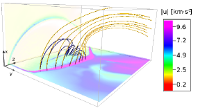
Figure 5.: Magnetic field lines connecting to the inside (dark blue) and to the outside (orange) of the fan-plane. The bottom slice shows the bulk speed at a height of about 1.4 Mm. The snapshot is taken at a displacement D = 2.15 Mm in the experiment run 3. The box size is $10\times 16\times 22$ Mm.fig:fieldline˙shear

The applied photospheric driving motion indirectly moves the fan-plane foot points at the west side of the fan-spine structure, causing a slight shear between the inner and the outer field lines of the fan-plane to arise due to a different stress level of these two flux systems. The magnetic flux system inside the dome experiences a compression of about 5 times the surrounding gas pressure when the magnetic flux system west to the dome has moved towards it. This leads to a large stress close to the null-point, on the east side of the outer spine, where the magnetic field as a consequence reconnects with the surrounding field in order to reach a lower energy state. A thin current sheet forms in the fan-plane, with the largest electric current densities occurring closest to the driver, where the shear of the field lines is largest. The magnitude of the electric current is lower in the neighborhood of the null-point. At the null-point itself the effect is to disrupt the structure of the null in such a way that the two spine axes move apart, as seen also in other single null investigations (Pontin, Bhattacharjee, and Galsgaard, 2007; Galsgaard and Pontin, 2011). Figure fig:j_fanplane shows the streamlines and direction of the highest electric current in run 3 at D = 2.68 Mm. We find that the electric current is mostly anti-parallel to the magnetic field lines in the fan-plane.

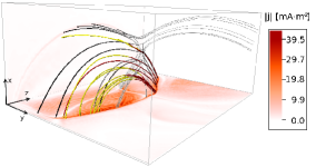
Figure 6.: The electric current (red–yellow) flowing antiparallel to the magnetic field lines (black–gray). The color gradient along the streamlines indicates the flow direction (going from red to yellow) and the magnetic field orientation (going from black to gray). The bottom slices show the electric current density of run 3. D = 2.68 Mm and the box size is $10\times 16\times 22$ Mm.fig:j˙fanplane

A partial outcome of the reconnection is seen in the motion of the inner spine, which is not being moved directly by the applied photospheric driver, but nevertheless moves at the photospheric level a significant absolute distance of about 4.5 Mm in the simulation. The motion is nearly linear in space and time. A second signature is the character of the displacement of the outer spine relative to the position of the inner spine.

The initial null-point area, connecting the inner and outer spine, stretches with increasing displacement into a ‘weak field region’, where the magnetic field strength is very low. This initiates an electric current that passes through the fan-plane, causing the ratio of the smallest to largest fan-eigenvalues to decrease (Parnell et al., 1996). In this case the null almost adopts a 2D structure. This is illustrated in Figure fig:bfield. We discuss the relation of this inner and outer spine distance to the electric field at the end of section sec:efield.

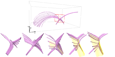
Figure 7.: Relative motion of inner and outer spine for run 3. The top panel shows the cutout region for D = 0.03 Mm and the lower panel shows approximately the same selected region for D = 0.03, 0.55, 1.08, 1.62, 2.15 Mm. The yellow volume indicates the highest electric current density, which is located in the fan-plane.fig:bfield

4.1 Time evolution of the diffusive electric fieldsec:efield

The diffusive part of the electric field ($\eta\textbf{j}$) included in the induction equation is responsible for both changing the magnetic field topology and for transforming magnetic energy into Joule dissipation in the MHD picture. In the Sun the diffusive electric field component parallel to the magnetic field is responsible for particle acceleration (Arzner and Vlahos, 2006). It is therefore of particular interest to see how this field evolves with the boundary displacement, and to find out where it concentrates and how large values it reaches. Figure fig:j_condense_strati_compare.ps illustrates the electric current accumulation in the fan-plane and along the spine axes of the magnetic null. This behavior is representative for all stratified and non-stratified runs. In the code the resistivity is not a simple constant, as specified by Equation (eq:nu), allowing diffusion to be locally increased where dissipation is needed to keep structures from becoming unresolved, while at the same time allowing a minimal amount of diffusion in regions where the magnetic field is smooth. Images of the diffusive electric field are therefore not exact replicas of images of the electric current, but since the resistivity is generally near its largest value in current sheets there is a close correspondence.

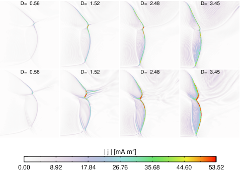
Figure 8.: Current density in y-z slice for constant density run 4 (upper row) and stratified atmosphere run 4S (lower row) at a height of x = 3.22 Mm and different displacements D.fig:j˙condense˙strati˙compare.ps

The diffusive electric field is found to be concentrated in the fan-plane and to have its local peak in the region where the fan-spine intersection is distorted. However, large values occur over a significant fraction of the fan-plane, as is the case for the electric current density.

It is only the parallel diffusive electric field that gives rise to both magnetic reconnection and particle acceleration and its magnitude indicates how violent these processes can be (Schindler, Hesse, and Birn, 1988). In our simulations the advective electric field ($-\mathbf{u}\times\textbf{B}$), associated with the bulk plasma motion in the fan-plane and along the spine axis is much stronger than its diffusive counterpart (Figure fig:electric_field_a), but since it is perpendicular to the magnetic field this component causes no magnetic dissipation, and cannot be associated with particle acceleration.

fig:electric_field_a

(a)

fig:electric_field_b

(b)

Figure 9.: Maximum advective electric field (a) and average diffusive electric field calculated over those grid points at which the electric field amplitude is within 10 % of the maximum field in a slice of 2 grid cells thickness (b) of the cutout region at the respective height of the null-point (*) and in the total cutout region $10\times 16\times 22$ Mm around the null-point, including the fan-plane (+) in run 3.fig:electric˙field

When determining the values of the diffusive electric field one finds that the peak values in the vicinity of the null-point are increasing with growing displacement (see Figure fig:electric_field_b), going from initially zero to on the order of 50 V m^-1, while in the fan-plane the diffusive electric field reaches more than 90 V m^-1 at D = 2.95 Mm. However, as shown below (cf. Equation eq:cs-efield and Equation eq:cs-efield2), to estimate the analogous solar electric field, the simulation value should be reduced with a factor equal to the power of 0.3 of the factor (about 20 for run 3) by which the boundary driving is exaggerated; here we obtain $E\approx 90/20^{0.3}$, or about 36 V m^-1. Considering our more benign conditions, this is consistent with Pudovkin et al. (1998), who find typical electric fields to be of the order of 100 – 300 V m^-1 under flaring conditions. Electrons accelerated along the entire current sheet, with an extent of about 15 Mm (see Figure fig:j_fanplane), could nevertheless gain energies of up to about 300 MeV in our case. Of interest is also the shape of the average diffusive electric field increase in the vicinity of the null-point, plotted in Figure fig:electric_field_b as a (*)-line. Its progression shows an almost identical behavior as a plot of the increasing distance between the inner and outer spine (see Figure fig:bfield) plotted against the displacement (plot not presented here).

4.2 Comparison of stratified and non-stratified simulations

Since the null-point is an essential node of the magnetic skeleton, we use it as a reference point for our investigation of the influence of the density profile on the temporal changes of the magnetic field. Here we compare simulation run 4S, which has a stratified atmosphere, with simulation run 4, which has a constant chromosphere-like density and temperature atmosphere (see, Table tab:simulations). Figure fig:nullpointpos shows the position of the null-point, connecting the fan-plane and spine magnetic field lines, in all three directions versus the boundary displacement D.

Figure 10.: Null-point position in Mm in the coordinate system of the experiment. The vertical coordinate is $x$, and the two horizontal coordinates are $y$ and $z$. The solid line shows the constant density run 4, while the dashed line represents the stratified run 4S.fig:nullpointpos

In the stratified case the very dense plasma ($9\times 10^{15}$ cm^-3) at the bottom of the box gives rise to a low Alfvén speed (v${}_{A}={B}/{\sqrt{\mu_{0}\rho_{m}}}$), meaning that the higher density impedes the propagation of the boundary disturbance into the box. But once the disturbances reach beyond the transition region the ambient density has fallen drastically, and the dense plasma from the lower atmosphere starts spreading out faster and pushes the null-point up. The velocity gradient induced by the large density change causes strong dissipation and in some regions a disruption into multiple smaller current sheets, which can also be seen in the electric current density comparison in Figure fig:j_condense_strati_compare.ps, showing $|j|$ for runs 4 and 4S.

In the non-stratified runs the amount of plasma that moves upwards along the magnetic field lines into the corona and contributes to pushing the null-point upwards is much reduced, as seen in Figure fig:nullpointpos.

For all runs we find a significant null-point motion (about 1–2 Mm in $x$, 6 Mm in $y$ and 1 Mm in $z$) due to the applied driving motion on the bottom boundary, which is comparable to the relative motion of the inner spine.

4.3 The influence of boundary conditions

The driver of the magnetic field evolution is the boundary motion. The magnetic field displacements imposed by the boundary motions have a large influence on the spatial structure of the magnetic skeleton, consisting of null-points, separatrix surfaces (such as the fan-plane), separators, sources and flux domains (e.g. Parnell, Haynes, and Galsgaard, 2008, and references therein). The skeleton itself is a very robust structure, which does not change from a topological point of view, but the detailed appearance of it changes with boundary displacement, as already shown by the analysis of the null-point motion.

In Figure fig:density_profile_b we compare the density profiles of the closed runs 1, 2, 3 and 4 and the open boundary run 1O. The figure shows that all non-stratified closed flow boundary runs develop a similar density profile: A certain expansion or compression of a region connected to the closed boundary leads to the same density profile, regardless of the driving speed.

The initial sound speed is about 83 km s^-1 for the non-stratified runs, while being much lower—on the order of 10 km s^-1—in the lower parts of the stratified runs. The sound speed influences among other things the in- and outflows at open boundaries.

fig:density_profile_a

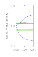
(a)

fig:density_profile_b

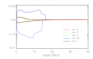
(b)

Figure 11.: Density profile min and max over each slice in height for the closed non-stratified simulations, normalized to the asymptote: run 1, run 2, run 3 and run 4 and the open non-stratified run 1O. (a) is a zoom in of the first 0.5 Mm of plot (b). The displacement of each run is taken to be from the snapshot closest to D = 1.05 Mm.fig:density˙profile.ps

Figure fig:density_profile_a illustrates that the closed boundary conditions influence particularly the lowest density layer, where regions with low and high density build up and cannot be emptied nor filled by plasma out- and inflow. This is not very important for the dynamics of the system, but is also not very solar-like. In the open case, there is a continuous mass exchange and pressure equalization at the boundaries, in which case it is crucial that the sound speed is well above the driving speed, so that the system has time to approach pressure balance.

The low sound speed in the stratified case poses a very tight restriction on the driving speed, in order to avoid exaggerating the effects of inertia. On the other hand there is a clear advantage of having stratification: it provides a pool of mass for the corona to communicate with; the large amount of mass at low temperature acts as a buffer, due to the low Alfvén and sound speed.

Overall, Figure fig:density_profile_b confirms that the density contrast is mainly caused by volume changes, which arise from the imposed boundary motions. If these volume changes happen sufficiently slowly relative to the Alfvén and sound speed, the driving speed loses its importance for the results (but not for the computational cost of obtaining them!).

4.4 Energy dissipation

As the boundary moves according to the prescribed driving pattern, with magnetic field lines passing through the boundary essentially ‘frozen in’, because of the boundary conditions, the system response may be mainly split into two distinct components. The first is the change in potential magnetic field energy due to the change of the vertical magnetic field component brought about by the boundary motions; this is the smallest amount by which the magnetic field energy could change. Secondly, in addition, the ‘free magnetic energy’ component will change as well. This non-potential part of the magnetic field is (by definition) associated with a non-zero electric current proportional to $\nabla\times\mathbf{B}$. The electric current may either be smooth and space-filling, or may be concentrated in electric current sheets, corresponding to near-discontinuities of the magnetic field.

Formally, the rate of change of magnetic energy density $e_{B}=B^{2}/2$ is described by Equation (equ:em), which shows that changes of magnetic energy are due to the net effect of a (negative) divergence of the Poynting flux $F_{P}$, conversion into bulk kinetic energy by the Lorentz work $W_{L}$, and conversion to heat through Joule dissipation $Q_{J}$.

$$\frac{\partial e_{B}}{\partial t}=-\nabla\cdot\mathbf{F}_{P}-W_{L}-Q_{J}.\ilabel{equ:em}$$ (17)

The Poynting flux is defined as $\mathbf{F}_{P}=\mathbf{E}\times\mathbf{B}$, and the Lorentz work is $W_{L}=\mathbf{u}\cdot(\textbf{j}\times\textbf{B})$. Joule dissipation, $Q_{J}=\mathbf{E}_{\eta}\cdot\mathbf{j}=\eta\mathbf{j}^{2}$, primarily takes place in the strong current sheets. Electric currents flow mainly along the magnetic field in the corona and therefore $Q_{J}$ is a suitable indicator for locations at which a significant component of the electric field parallel to the magnetic field may exist. Such a parallel electric field can accelerate charged particles along the magnetic field lines, resulting e.g. in the brightening of flare ribbons.

The evolutions of the magnetic energy and the Joule dissipation normalized to the average driving speed are summarized in a plot covering several simulation runs in Figure fig:plot_joule_magnenergy.ps.

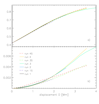
Figure 12.: Comparison of the average magnetic energy a) and average magnetic dissipation divided by the normalized (v₀ = 10 km s^-1) average boundary driving speed of each run b) for constant density runs (solid lines) and stratified runs (dashed lines) in the cutout of approximate size 10 x 16 x 22 Mm.fig:plot˙joule˙magnenergy.ps

The first thing to notice is that the evolution of the magnetic energy, when expressed in terms of the boundary displacement $D$, is practically identical in all of the runs. The reason for this is that most of the boundary work goes directly into increasing the potential magnetic energy, while only a small amount goes into free magnetic energy. From Figure fig:plot_joule_magnenergy.psb is seen that the dissipation increases with increasing displacement. This indicates that an increasing amount of free energy becomes available through the build up of current structures in the null-point fan-plane as the experiment progresses.

A comparison between different power-law relations indicates, that the normalization of the magnetic dissipation by the average normalized driving speed to the power 0.6 employed in Figure fig:plot_joule_magnenergy.psb brings the curves showing the evolution of magnetic dissipation for all the different runs closest together into a relatively tight set of parallel relations. This illustrates that the rate of magnetic dissipation, at any given value of the displacement, is approximately proportional to the rate of boundary displacement to the power 0.6.

The dissipation curves corresponding to the different experiments follow the same general trend, although with some differences, in particular between the stratified and non-stratified cases. The dissipation is generally higher for the stratified cases than for the non-stratified runs during early times and lower during late times. The exception is run 1S, the run with the lowest driving speed, which agrees closely with the non-stratified cases with the slowest driving speed.

The deviations from this common asymptotic behavior are likely consequences of the low Alfvén speeds in the dense layers of the stratified models, causing the dissipation in the stratified runs to be initially high due to their higher densities at low heights compared to the constant density cases. Later, when the motions introduced by the driver reach greater heights, where the mass density is lower than in the constant density runs, the stratified runs generally display a lower dissipation.

We note in this context also that the viscous dissipation in the system is much smaller than the Joule dissipation, as is expected in a coronal environment.

The results summarized in Figure fig:plot_joule_magnenergy.ps illustrate that for a quantitatively accurate estimate of properties related to the magnetic dissipation it is essential to drive in a way which is compatible with the ordering of characteristic speeds in the Sun; i.e., to keep the boundary speed smaller than the Alfvén speed, and to scale the quantities down in proportion to the speed-up factor used in the driving.

For the non-stratified runs we compute initial Alfvén speeds of 70 – 1400 km s^-1 at the lower boundary, which is clearly higher than the driving speed of all runs. So we expect, as is also shown by Figure fig:plot_joule_magnenergy.ps, a similar dissipation increase with increasing displacement, after some initial differences due to the driving speed differences.

In the stratified atmosphere runs the Alfvén speed increases with height. At the lower boundary the initial Alfvén speed is approximately 5 – 200 km s^-1, where the minimum value falls below the driving speed used in runs 3S and 4S. Run 1S is just at the edge of being driven slower than the minimum Alfvén speed and indeed gives results which are similar to the non-stratified case run 1. Figure fig:dissipation_run4 shows that the stratified and non-stratified cases are nevertheless distinguishable. The volume renderings show the Joule dissipation normalized by the driving speed, for run 1 (upper panel) and run 1S (lower panel). The locations of the dissipation maxima agree nicely, but the dissipation maxima differ by a factor of about 1.8, being higher in the stratified run 1S.

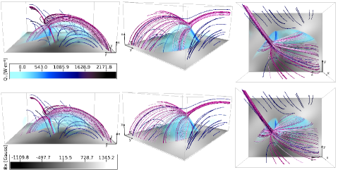
Figure 13.: The highest joule dissipation of run 1 in the top row and run 1S in the lower row is shown as a semitransparent volume rendering at about D = 0.88 Mm. The box size is $10\times 16\times 22$ Mm. The field lines represent magnetic field lines passing closest to the null point (purple), in the close surrounding of the null-point (magenta) and the overlying strong magnetic field (dark blue). The slice on the lower boundary shows the Bx magnetic field component. fig:dissipation˙run4

In summary, we find that the ratio of the driving speed to the Alfvén speed has a noticeable impact on the dissipation level and, as Figure fig:plot_joule_magnenergy.ps illustrates, that the stratified simulations tend to display a progressive growth of deviations from the common asymptotic relations defined by the non-stratified runs, unless the driving speed is small compared to both the local Alfvén speed and the sound speed.

However, these are relatively small deviations, compared to the main trend, which is a proportionality between the magnetic dissipation and the driving speed to the power 0.6.

4.5 Scaling of magnetic dissipation in the current sheet

As illustrated by Figure fig:fieldline_shear, the magnetic field line orientations on the two sides of the fan-plane only differ by a small amount. This means that the electric current carried by the current sheet, whose thickness (on the order of a few grid cells in the present numerical model) we denote with $\Delta s$, is much less than the maximal electric current density $2B/\Delta s$ that would result from a complete reversal of the magnetic field orientation across the current sheet. The electric current density in the current sheet (CS) is in fact on the order of

$$j_{{\rm CS}}\sim\Delta B\;\Delta s^{-1}\approx sin(\phi)B_{{\rm CS}}\Delta s^{-1}\approx\phi B_{{\rm CS}}\Delta s^{-1},\ilabel{eq:cs-current}$$ (18)

for small $\phi$, where $B_{{\rm CS}}$ is a typical strength of the magnetic field just outside the current sheet, and $\phi$ is an angle characterizing the difference of direction of field lines on the two sides of the current sheet.

A fundamental question is now how the total dissipation in the current sheet, and hence the average rate of reconnection in the structure, depends on factors such as the numerical resolution and rate of work done at the boundary. By construction the code keeps current sheets just barely resolved. A change in numerical resolution is thus directly mapped into a proportional change of the current sheet thickness $\Delta s$. This behavior is obtained by making $\eta$ essentially proportional to the grid size (cf. Equation eq:eta). To a first order approximation both $B_{{\rm CS}}$ and $\phi$ are independent of $\Delta s$. By Equation eq:cs-current the electric current density is inversely proportional to $\Delta s$, and the magnetic dissipation rate per unit volume $Q_{J}$ therefore scales as

$$\ilabel{eq:cs-dissipation}Q_{{\rm CS}}=\eta j_{CS}^{2}\sim\Delta B^{2}\Delta s^{-1}=\phi^{2}B_{CS}^{2}\Delta s^{-1}.\ilabel{eq:dissipation_{C}S}$$ (19)

To obtain the total dissipation in the current sheet this needs to be multiplied with the volume of the current sheet,

$$\ilabel{eq:cs-volume}V_{{\rm CS}}\sim A_{{\rm CS}}\Delta s,$$ (20)

where we denote by $A_{{\rm CS}}$ the total area of the current sheet. We thus conclude that the total dissipation is

$$\ilabel{eq:cs-dissipation2}Q_{{\rm CS}}V_{{\rm CS}}\sim\Delta B^{2}A_{{\rm CS}},$$ (21)

and hence is, to lowest order, independent of $\Delta s$ and the resistivity in the current sheet. Note that, as a consequence of $\phi$ being small, reconnection in the current sheet can proceed without requiring super-Alfvénic outflow velocities from the current sheet.

Estimating now the diffusive electric field in the current sheet we find that it scales as

$$\ilabel{eq:cs-efield}E_{{\rm CS}}=\eta_{{\rm CS}}j_{{\rm CS}}\propto\Delta B=\phi B_{{\rm CS}},\ilabel{eq:resistive_{e}field}$$ (22)

again independent of $\Delta s$, but proportional to the change of magnetic field direction across the current sheet and hence proportional to $\phi$.

Generally the work done by the boundary must go into an increase in magnetic energy (potential plus free magnetic energy), or into kinetic energy or ohmic dissipation. In the present case the magnetic dissipation is able to nearly keep up with the free energy input, and the system essentially goes through a series of states not far from potential. As Figure fig:plot_joule_magnenergy.ps shows, the total magnetic energy depends mainly on the displacement and very little on the driving speed itself, while the dissipation is essentially proportional to how fast we drive at the boundary to the power of 0.6, thus $Q_{{\rm CS}}\propto v^{0.6}$. So we conclude with the help of Equations (eq:dissipation_CS) and (eq:resistive_efield) that the magnitude of the parallel electric field along the current sheet scales as

$$\ilabel{eq:cs-efield2}E_{{\rm CS}}\propto\phi\propto v^{0.3}.$$ (23)

This electric field – driving speed relation is not an artifact of the chosen numerical method; the scaling of $\eta$ with $\Delta s$ is generic to all numerical methods, and serves to ensure that higher numerical resolution can be used to reach larger magnetic Reynolds and Lundquist numbers.

With much higher rates of stressing, or with much higher numerical resolution, the current sheet may need to fragment and enter a turbulent regime, in order to support the required amounts of dissipation and reconnection in the face of increasing constraints by the thinness of the current sheets. This is a process that is by now well understood to be able to take over when the need arises (Galsgaard and Nordlund, 1996; Nordlund and Galsgaard, 1997b; Gudiksen and Nordlund, 2005; Berger and Asgari-Targhi, 2009; Bingert and Peter, 2011; Ng, Lin, and Bhattacharjee, 2012; Pontin, 2011).

We thus conclude that, provided that conditions that apply equally to both numerical simulations and the Sun are fulfilled, neither the total magnetic dissipation in a current sheet structure, nor the diffusive part of the electric field depend, to lowest order, on the electrical resistivity—or for that matter on the precise mechanism that sets the level of the electrical resistivity.

4.6 Triggering of rapid energy release

As in Masson et al. (2009) there is no significant and sudden relaxation of the system, with an energy release that could correspond to a flare, even though the simulations cover enough solar time to get across the observed flaring event. Looking at the potential part of the magnetic field at different displacement steps in the simulations, we find steadily increasing magnetic potential energies, and most of the build-up of magnetic energy seen in the experiment actually goes into increasing the potential rather than the non-potential part of the magnetic energy. As discussed above, the magnetic dissipation is able to keep up with varying levels of boundary work, with a residual amount of free energy scaling, if it is proportional to the rate of dissipation, approximately as the driving speed raised to 0.6. The stress in the system is demonstrably moderate, even with our exaggerated driving speed, and we therefore cannot expect boundary motions of the type applied here to be able to explain violent events similar to the observed solar flare.

We consider four possibilities for this difference in behavior between these MHD simulations and the Sun:

1. The limited resolution of the numerical experiment is preventing an instability from occurring that would otherwise trigger a flare-like event.

2. A flare-like event would occur if taking into account kinetic effects (e.g. by using particle-in-cell simulations).

3. A flare-like event could take place, with MHD alone, but would require an additional Poynting flux through the boundary, in addition to the Poynting flux generated by the simple driver implemented here and in Masson et al. (2009).

4. The additional free energy available because the system was initially not in a potential state could have helped.

As demonstrated above, numerical resolution does not to a first order determine the level of dissipation in current sheets, once they are reasonably well resolved. Indeed, by the arguments in the preceding subsection we expect the level of stress (as measured for example by the angle $\phi$) caused by the type of motions we employ in the current investigation to be smaller in the Sun (by a factor of e.g. $\approx 7^{0.3}\approx 2$ relative to our runs 1, 1O and 1S), and it is thus very unlikely that the flare was triggered by accumulation of stress from this particular type of boundary motion.

An MHD-instability could in principle occur at a later point in time than to where our runs go; but as demonstrated by our experiments even a driving speed that is highly exaggerated relative to the solar value is not able to build up sufficient free energy to account for a C-class flare: The maximum total magnetic energy in the entire simulated domain of our experiment is on the order of $2\times 10^{30}$ ergs, of which only a very small fraction is free energy. Estimates of C-flare emission are larger than even our potential energy (Kretzschmar, 2011), and hence the free energy available in our model is not sufficient to power a C-class flare. As discussed above, the level of stress is expected to be proportional to the driving speed to some small positive power, and is expected to be largely independent of the level of resistivity, and hence it is unlikely that more stress would build up in the Sun than in these numerical simulations.

Figure fig:plot_joule_magnenergy_time.ps, which is representative of all runs, illustrates that the rate of change of magnetic energy increases in the beginning, as a result of the work done by the lower boundary. This energy input loses efficiency as the angle between the field lines and the driving boundary approaches 90 degrees. Additionally, since the driving pattern location is fixed, the applied stress becomes less and less efficient, as the flux in this particular region is gradually removed. The dissipation is small compared to the rate of change of magnetic energy, implying that the dissipated free energy only makes up a tiny fraction compared to the change of the potential energy. This is in agreement with Figure fig:fieldline_shear, which illustrates that the shear of the magnetic field lines in the current sheet is not very large, even with our exaggerated driving speed. Hence the reconnection is rapid enough to keep the boundary work at a given displacement at an approximately constant level, and to keep the system in a near potential state. We are thus far away from an instability to occur and it is improbable to achieve one at a later point of the experiment with the applied boundary motion. The mostly compressive boundary driving pattern probably does not represent reality accurately enough, and additional shearing, twisting, or emerging motions may have been present.

Figure 14.: The average rate of change of magnetic energy for run 3 is plotted as a solid line, and the dissipation is shown as a dashed line. Both are restricted to the cutout of approximate size 10 x 16 x 22 Mm used previously.fig:plot˙joule˙magnenergy˙time.ps

By similar arguments kinetic effects are not expected to have a major influence on the macroscopic dissipation behavior and reconnection rate. This is consistent with the findings by Birn et al. (2005), which show that the same amounts of energy release take place for the same type of reconnection event, independent of the dissipation mechanism. It also shows that there are only small differences in the time scales of the event going from MHD to PIC simulations. These results are entirely consistent with the current sheet scaling arguments presented above, since they hold true independent of the nature of the dissipation mechanism.

We thus are left with the option that the additional free energy mentioned in the third and forth alternative above is the most likely explanation for the observed solar flare. This conclusion is consistent with the fact that all observational evidence associates flaring either with new flux emergence, or with magnetic configurations that evolve into states that are decidedly MHD-unstable; i.e., ones in which lower energy states become accessible and where dissipative effects make it possible to reach those lower energy states and dynamic instabilities therefore develop. Some amount of free magnetic energy was clearly present in the system at the time where we are forced by circumstances to assume a potential initial state. Whether that extra free energy alone would have been enough to cause a flare several hours later is an open question. Our driver pattern might have been able to add slightly more magnetic energy to a configuration that already contained free magnetic energy, but that effect is probably small. We consider the addition of Poynting flux, increasing the free magnetic energy of the system at a considerably higher rate than can be achieved with our driver pattern as the more likely alternative. Additional Poynting flux across the lower boundary can take the form of either emerging flux (Poynting flux due to vertical velocity) or twisting boundary motions (Poynting flux due to vortical horizontal velocity).

As evidence for this view, we consider magnetograms starting on November 12, 2002 in the early afternoon, when a strong negative polarity first appeared within the positive polarity. The negative polarity expanded and several eruptions could be seen at EUV wavelengths. During the interval simulated here one observes an additional increase in the negative flux inside the dome, and there are also other significant rearrangements that our driver pattern is not able to represent or explain.

5 Conclusions

sec:conclusions The main topic of the presented work is a study of the influence of the driving speed for stratified and non-stratified atmosphere models used to simulate 3D reconnection events in the solar corona. The major findings are:

• Sufficiently low driving speeds lead to similar plasma behavior, including similar evolution of the magnetic energy density (after compensating for the expected effects of the different driving speeds).

• The magnetic dissipation and the diffusive electric field — capable of accelerating charged particles depend only weakly on the grid resolution in the numerical experiments.

• When driving is taking place sufficiently slowly, the rate of magnetic dissipation increases approximately as the boundary driving speed raised to the power 0.6 while the diffusive electric field increases approximately as the driving speed raised to the power 0.3.

• The driving speed has a larger impact on the general plasma behavior in the cases with stratified atmospheres, while its influence is minor for non-stratified runs with closed flow boundary conditions, if compared at the same boundary motion displacements.

• The sound speed compared to the driving speed determines the exchange of plasma at the boundaries. Voids can be filled in open boundary runs, while pressure differences at the boundary are carried along in the closed boundary cases. This is not an issue in the stratified runs, due to the large reservoirs of relatively cold gas in the vicinity of the lower boundary. On the other hand, the lower information speeds there set severe restrictions on the driving speed.

Our investigations suggest that the applied simple driver pattern is unlikely to be able to cause a flare-like energy release in the simulations (as well as in the Sun). In fact, based on a comparison of the available free energy in our model with estimates from observations of C-class flares we anticipate that the corresponding solar configuration must have had significantly more free magnetic energy added through the boundary, or must otherwise have been in a strongly non-potential state already before the studied time interval.

Acknowledgements

We would like to especially thank Jacob Trier Frederiksen and Troels Haugbølle for valuable discussions and for their assistance with the simulations. We thank Guillaume Aulanier and Sophie Masson for providing us with their MHD data and driver information. We also thank the referee for useful comments and criticism. This work has been supported by the Niels Bohr International Academy and the SOLAIRE Research Training Network of the European Commission (MRTN-CT-2006-035484). The work of ÅN was partially supported by the Danish Research Council for Independent Research (FNU) and the funding from the European Commission’s Seventh Framework Programme (FP7/2007-2013) under the grant agreement SWIFF (project n 263340, www.swiff.eu). The data for the magnetic field extrapolation were taken from the SOHO catalog. SOHO is a project of international cooperation between ESA and NASA. We furthermore acknowledge that the results in this paper have been achieved using resources at the Danish Center for Scientific Computing in Copenhagen, as well as PRACE and GCS/NIC Research Infrastructure resources on JUGENE and JUROPA based at Jülich in Germany.

References

- Archontis et al. (2004) Archontis, V., Moreno-Insertis, F., Galsgaard, K., Hood, A., O’Shea, E.: 2004, Emergence of magnetic flux from the convection zone into the corona. A&A 426, 1047 – 1063. doi:10.1051/0004-6361:20035934.
- Arzner and Vlahos (2006) Arzner, K., Vlahos, L.: 2006, Gyrokinetic electron acceleration in the force-free corona with anomalous resistivity. A&A 454, 957 – 967. doi:10.1051/0004-6361:20064953.
- Berger and Asgari-Targhi (2009) Berger, M.A., Asgari-Targhi, M.: 2009, Self-organized Braiding and the Structure of Coronal Loops. ApJ 705, 347 – 355. doi:10.1088/0004-637X/705/1/347.
- Bingert and Peter (2011) Bingert, S., Peter, H.: 2011, Intermittent heating in the solar corona employing a 3D MHD model. A&A 530, A112. doi:10.1051/0004-6361/201016019.
- Birn et al. (2005) Birn, J., Galsgaard, K., Hesse, M., Hoshino, M., Huba, J., Lapenta, G., Pritchett, P.L., Schindler, K., Yin, L., Büchner, J., Neukirch, T., Priest, E.R.: 2005, Forced magnetic reconnection. Geophys. Res. Lett. 32, 6105. doi:10.1029/2004GL022058.
- Fan and Gibson (2003) Fan, Y., Gibson, S.E.: 2003, The Emergence of a Twisted Magnetic Flux Tube into a Preexisting Coronal Arcade. ApJ 589, L105 – L108. doi:10.1086/375834.
- Galsgaard and Nordlund (1996) Galsgaard, K., Nordlund, Å.: 1996, Heating and activity of the solar corona 1. Boundary shearing of an initially homogeneous magnetic field. J. Geophys. Res. 101, 13445 – 13460. doi:10.1029/96JA00428.
- Galsgaard and Pontin (2011) Galsgaard, K., Pontin, D.I.: 2011, Steady state reconnection at a single 3D magnetic null point. A&A 529, A20. doi:10.1051/0004-6361/201014359.
- Green (1989) Green, J.M.: 1989, Geometrical properties of 3d reconnecting magnetic fields with nulls. J. Geophys. Res. 93, 8583.
- Gudiksen and Nordlund (2002) Gudiksen, B.V., Nordlund, Å.: 2002, Bulk Heating and Slender Magnetic Loops in the Solar Corona. ApJ 572, L113 – L116. doi:10.1086/341600.
- Gudiksen and Nordlund (2005) Gudiksen, B.V., Nordlund, Å.: 2005, An Ab Initio Approach to the Solar Coronal Heating Problem. ApJ 618, 1020 – 1030. doi:10.1086/426063.
- Hyman (1979) Hyman, J.M.: 1979, A method of lines approach to the numerical solution of conservation laws. In: Advances in Computer Methods for Partial Differential Equations - III, 313 – 321.
- Kretzschmar (2011) Kretzschmar, M.: 2011, The Sun as a star: observations of white-light flares. A&A 530, A84. doi:10.1051/0004-6361/201015930.
- Kritsuk et al. (2011) Kritsuk, A.G., Nordlund, Å., Collins, D., Padoan, P., Norman, M.L., Abel, T., Banerjee, R., Federrath, C., Flock, M., Lee, D., Li, P.S., Müller, W.-C., Teyssier, R., Ustyugov, S.D., Vogel, C., Xu, H.: 2011, Comparing Numerical Methods for Isothermal Magnetized Supersonic Turbulence. ApJ 737, 13. doi:10.1088/0004-637X/737/1/13.
- Masson et al. (2009) Masson, S., Pariat, E., Aulanier, G., Schrijver, C.J.: 2009, The Nature of Flare Ribbons in Coronal Null-Point Topology. ApJ 700, 559 – 578. doi:10.1088/0004-637X/700/1/559.
- Ng, Lin, and Bhattacharjee (2012) Ng, C.S., Lin, L., Bhattacharjee, A.: 2012, High-Lundquist Number Scaling in Three-dimensional Simulations of Parker’s Model of Coronal Heating. ApJ 747, 109. doi:10.1088/0004-637X/747/2/109.
- Nordlund and Galsgaard (1997a) Nordlund, A., Galsgaard, K.: 1997a, A 3D MHD code for Parallel Computers. Technical report, Niels Bohr Institute.
- Nordlund and Galsgaard (1997b) Nordlund, A., Galsgaard, K.: 1997b, Topologically Forced Reconnection. In: Simnett, G.M., Alissandrakis, C.E., Vlahos, L. (eds.) European Meeting on Solar Physics, Lecture Notes in Physics, Berlin Springer Verlag 489, 179. doi:10.1007/BFb0105676.
- Parnell, Haynes, and Galsgaard (2008) Parnell, C.E., Haynes, A.L., Galsgaard, K.: 2008, Recursive Reconnection and Magnetic Skeletons. ApJ 675, 1656 – 1665. doi:10.1086/527532.
- Parnell et al. (1996) Parnell, C.E., Smith, J.M., Neukirch, T., Priest, E.R.: 1996, The structure of three-dimensional magnetic neutral points. Physics of Plasmas 3, 759 – 770. doi:10.1063/1.871810.
- Pontin (2011) Pontin, D.I.: 2011, Three-dimensional magnetic reconnection regimes: A review. Advances in Space Research 47, 1508 – 1522. doi:10.1016/j.asr.2010.12.022.
- Pontin, Bhattacharjee, and Galsgaard (2007) Pontin, D.I., Bhattacharjee, A., Galsgaard, K.: 2007, Current sheet formation and nonideal behavior at three-dimensional magnetic null points. Physics of Plasmas 14(5), 052106. doi:10.1063/1.2722300.
- Priest and Titov (1996) Priest, E.R., Titov, V.S.: 1996, Magnetic Reconnection at Three-Dimensional Null Points. Royal Society of London Philosophical Transactions Series A 354, 2951 – 2992. doi:10.1098/rsta.1996.0136.
- Priest, Bungey, and Titov (1997) Priest, E.R., Bungey, T.N., Titov, V.S.: 1997, The 3D topology and interaction of complex magnetic flux systems. Geophysical and Astrophysical Fluid Dynamics 84, 127 – 163. doi:10.1080/03091929708208976.
- Pudovkin et al. (1998) Pudovkin, M.I., Zaitseva, S.A., Shumilov, N.O., Meister, C.-V.: 1998, Large-Scale Electric Fields in Solar Flare Regions. Sol. Phys. 178, 125 – 136.
- Scherrer et al. (1995) Scherrer, P.H., Bogart, R.S., Bush, R.I., Hoeksema, J.T., Kosovichev, A.G., Schou, J., Rosenberg, W., Springer, L., Tarbell, T.D., Title, A., Wolfson, C.J., Zayer, I., MDI Engineering Team: 1995, The Solar Oscillations Investigation - Michelson Doppler Imager. Sol. Phys. 162, 129 – 188. doi:10.1007/BF00733429.
- Schindler, Hesse, and Birn (1988) Schindler, K., Hesse, M., Birn, J.: 1988, General magnetic reconnection, parallel electric fields, and helicity. J. Geophys. Res. 93, 5547 – 5557. doi:10.1029/JA093iA06p05547.