Cosmology with clustering anisotropies: disentangling dynamic and geometric distortions in galaxy redshift surveys

Abstract

We investigate the impact of different observational effects affecting a precise and accurate measurement of the growth rate of fluctuations from the anisotropy of clustering in galaxy redshift surveys. We focus here on redshift measurement errors, on the reconstruction of the underlying real-space clustering and, most importantly, on the apparent degeneracy existing with the geometrical distortions induced by the cosmology-dependent conversion of redshifts into distances. We use a suite of mock catalogues extracted from large N-body simulations, focusing on the analysis of intermediate, mildly non-linear scales ($r<50$$h^{-1}\,\mbox{Mpc}$ ) and apply the standard “dispersion model” to fit the anisotropy of the observed correlation function $\xi(r_{\perp},r_{\parallel})$ . We first verify that redshift errors up to $\delta z\sim 0.2\%$ (i.e. $\sigma_{z}\sim 0.002$ at $z=1$) have a negligible impact on the precision with which the specific growth rate $\beta$ can be measured. Larger redshift errors introduce a positive systematic error, which can be alleviated by adopting a Gaussian distribution function of pairwise velocities. This is, in any case, smaller than the systematic error of up to $10\%$ due to the limitations of the dispersion model, which is studied in a separate paper. We then show that $50\%$ of the statistical error budget on $\beta$ depends on the deprojection procedure through which the real-space correlation function, needed for the modelling process, is obtained. Finally, we demonstrate that the degeneracy with geometric distortions can in fact be circumvented. This is obtained through a modified version of the Alcock-Paczynski test in redshift-space, which successfully recovers the correct cosmology by searching for the solution that optimizes the description of dynamical redshift distortions. For a flat cosmology, we obtain largely independent, robust constraints on $\beta$ and on the mass density parameter, $\Omega_{\rm M}$ . In a volume of $2.4(h^{-1}\,\mbox{Gpc})^{3}$, the correct $\Omega_{\rm M}$ is obtained with $\sim 12\%$ error and negligible bias, once the real-space correlation function is properly reconstructed.

1 Introduction

The large scale structure of the Universe is one of the main observational probes to discriminate among competing cosmological models and estimate their fundamental parameters, some related to space-time geometry, some related to the density fluctuations. The growth rate of density fluctuations, $f(z)$, belongs to the second category. Since the pioneering works of Kaiser (1987) and Hamilton (1998), it was clear that one of the most promising ways to determine $f(z)$ is to exploit the apparent anisotropy in the clustering of galaxies induced by peculiar velocities, an effect commonly known as redshift-space distortions (RSD).

Being $f(z)$ directly sensitive to the mean density of matter, for some time RSD have been used to estimate the mass density parameter $\Omega_{\rm M}$ (e.g. Peacock et al., 2001; Hawkins et al., 2003; da Ângela et al., 2005a, b; Ross et al., 2007; Ivashchenko et al., 2010). Later on, with the advent of other, more precise methods to estimate $\Omega_{\rm M}$ , like the Barionic Acoustic Oscillations (BAO), RSD began to be considered as a sort of “noise” to be marginalized over (Seo & Eisenstein, 2003, 2007). New interest on RSD arose when it was realized that, if not marginalized over, they could tighten constraints over cosmological parameters (Amendola et al., 2005), and in particular when it was shown (Guzzo et al., 2008; Zhang et al., 2008) that they could represent a formidable tool to discriminate between a dark energy (DE) scenario and a modified gravity theory for the origin of cosmic acceleration. A number of forecast papers followed rapidly (e.g. Linder, 2008; Wang, 2008; Song & Percival, 2009), as well as applications to existing and new datasets (Cabré & Gaztañaga, 2009a, b; Blake et al., 2011). As such, RSD are now regarded as one of the most promising techniques to extract precise estimates of $f(z)$ from future redshift surveys. Besides their use as a probe to constrain alternative gravity theories, RSD can also be exploited in many different contexts. For instance, it has been recently demonstrated that RSD robustly constrain the mass of relic cosmological neutrinos (Marulli et al., 2011) and could be used to detect interactions in the dark sector (Marulli et al., 2012). Moreover, they can be of some help in astrophysical contexts, e.g. to investigate the dynamical properties of the warm-hot intergalactic medium (Ursino et al., 2011).

To effectively discriminate among competing cosmological models, however, one needs to measure the growth rate with per cent accuracy. This goal has prompted several works aimed at better identifying and characterizing the sources or uncertainty. One aspect of the problem is how to optimally infer the growth rate of fluctuations from the measured RSD quantities. The anisotropic pattern of galaxy redshifts in 3D space allows one to estimate the distortion parameter $\beta(z)\equiv f(z)/b(z)$. Then, to obtain $f(z)$, one needs in principle an independent estimate of the galaxy bias parameter $b(z)$ which is ill-constrained by theory and difficult to measure from the data. For this reason, it has been suggested (see e.g. White et al., 2009; Percival & White, 2009; Song & Percival, 2009) to express the constraints in terms of the observed product $\beta(z)\sigma^{gal}_{8}(z)$, which in the linear bias hypothesis equals the theoretical combination $f(z)\sigma_{8}(z)$. In these expressions $\sigma^{gal}_{8}$ and $\sigma_{8}$ are the rms values in spheres of 8 $h^{-1}\,\mbox{Mpc}$ of respectively the galaxy counts and the mass. In this way, the values of $\beta(z)\sigma^{gal}_{8}(z)$ obtained from the data at different redshifts can be self-consistently compared to the curves $f(z)\sigma_{8}(z)$ predicted by the theory (once they are nevertheless normalized to a reference $\sigma_{8}$ as provided, e.g., by CMB measurements).

Another aspect of the problem is the impact of the observational errors, related to redshift measurements and to the nature of the objects used to trace the mass inhomogeneities. This is commonly addressed using the Fisher information matrix (Fisher, 1935; Tegmark et al., 1997), which has become the standard method to forecast statistical errors in the cosmological parameters expected from planned redshift surveys (see e.g. Sapone & Amendola, 2007; Wang, 2008; Linder, 2008; White et al., 2009; Percival & White, 2009; Wang et al., 2010; Acquaviva & Gawiser, 2010; Fedeli et al., 2011; Carbone et al., 2011a, b, 2012; Di Porto et al., 2012a, b; Majerotto et al., 2012). One limitation in the use of the Fisher matrix is that it relies on assumptions (e.g. the Gaussian nature of errors) that in some applications might not be fully justified. In addition, the Fisher matrix formalism cannot say anything about systematic errors that may dominate the error budget in future experiments aiming at per cent accuracy. Finally, the use of the Fisher matrix is justified on large scales, where linear theory applies, but may fail on smaller scales because of the improper treatment of deviations from linearity in dynamics and bias. In all these cases one needs to use numerical simulations.

Early attempts to test the accuracy of the linear model of RSD (Kaiser, 1987) through numerical simulations and develop improved corrections (Scoccimarro, 2004; Tinker et al., 2006) have been recently extended, following the renewed interest on this topic (Taruya et al., 2011; Jennings et al., 2011a, b; Okumura & Jing, 2011; Kwan et al., 2012; Samushia et al., 2011). The work presented here is part of this ongoing effort to understand the limitations of RSD estimators and bring this technique at the level required by precision cosmology.

Finally, a potentially relevant source of systematic error in the measurement of RSD is related to intrinsic uncertainty on the background cosmology, which is needed when converting redshifts into distances. This introduces further geometric distortions (GD) in the observed clustering pattern, which in principle can be used to estimate the background cosmological parameters through the so-called Alcock-Paczynski (AP) test (Alcock & Paczynski, 1979). Several methods and attempts to implement the AP test using different datasets have been proposed (Alcock & Paczynski, 1979; Phillipps, 1994; Ryden, 1995; Ryden & Melott, 1996; Marinoni & Buzzi, 2010), including those that look for anisotropies in 3D clustering (Ballinger et al., 1996; Matsubara & Suto, 1996; Popowski et al., 1998; Hui et al., 1999; Matsubara, 2000; McDonald, 2003; Nusser, 2005; Barkana, 2006; Kim & Croft, 2007; Padmanabhan & White, 2008). In practice, GD have a smaller amplitude than and are degenerate with RSD (Simpson & Peacock, 2010), such that only with very high quality data one can hope to disentangle the two effects. Early applications of the AP test thus failed to get significant results (Outram et al., 2004; Hoyle et al., 2002; da Ângela et al., 2005a, b; Ross et al., 2007), but the situation is rapidly improving (Chuang & Wang, 2012; Blake et al., 2011). It is fairly clear that GD will play a fundamental role in the estimate of cosmological parameters from future surveys (Seo & Eisenstein, 2003; Simpson & Peacock, 2010; Kazin et al., 2012; Taruya et al., 2011; Samushia et al., 2012; Hawken et al., 2012), but also that, if not properly accounted for, they represent one further source of systematic error in the measurement of $f(z)$ from RSD.

In this paper we explore how the precision and accuracy of $f$ depend on the limitations of i) using observed quantities (angles and redshift) to infer cosmological distances in redshift-space, and ii) using them to construct and model two-point statistics. We therefore first assess the impact on the recovered $\beta$ of redshift measurement errors and of the intrinsic uncertainty on the real-space two-point correlation function due to the deprojection procedure. We then look in detail into the effect of GD and introduce a simple technique to isolate RSD. We show that, under the hypothesis of a flat background, this allows us to simultaneously measure $\beta$ and $\Omega_{\rm M}$. Finally, we relax the flat background assumption and investigate how GD can be used to constrain the cosmological parameters that enter the Hubble function. These tests focus on intermediate scales ($r<50$$h^{-1}\,\mbox{Mpc}$ ), where non-linear effects cannot be neglected. These are the scales where RSD have the highest signal-to-noise, also in last-generation surveys like WiggleZ (Blake et al., 2011), VIMOS Public Extragalactic Redshift Survey (Guzzo et al., in preparation, VIPERS) and SDSS-III BOSS (Eisenstein et al., 2011).

In a parallel, complementary work (Bianchi et al., 2012), we use the same numerical methods adopted here to study the dependence of the uncertainty on the measured growth rate on typical survey parameters, as the volume and the density and bias of the adopted tracers.

The paper is organised as follows. In §2 we start describing the exploited set of N-body simulations and how to construct mock halo catalogues. Then we give a general overview on RSD and GD. In §3 we investigate the impact of redshift errors, deprojection effects and geometric uncertainties on the estimate of the RSD parameters. The method to disentangle GD and RSD is analysed in §4. Finally, in §5, we draw our conclusions.

2 Theoretical tools

In this section we review the theoretical tools we use to derive the random and systematic errors in the estimate of $f(z)$ from RSD. Since we are not concerned on galaxy bias, we will focus on the distortion parameter $\beta$.

2.1 N-body simulations and mock halo catalogues

Since we are interested in RSD on intermediate scales, our analysis will rely on mock catalogues extracted from N-body simulations that fully account for non-linear dynamics. The need for a sufficiently large number of independent mock catalogues, each one with a volume matching that of the typical ongoing redshift surveys, imposes to consider very large computational boxes.

The ‘Baryon Acoustic Simulation at the ICC’, BASICC, meets these requirements (Angulo et al., 2008). This simulation follows the dynamical evolution of $1448^{3}$ dark matter (DM) particles with mass $M_{\rm part}=5.49\times 10^{10}\,h^{-1}{\rm M}_{\odot}$ in a box of $1340$ $h^{-1}\,\mbox{Mpc}$ , using a memory-efficient version of the GADGET-2 code (Springel, 2005). The cosmological model adopted is a $\Lambda$CDM universe with $\Omega_{\rm M}=0.25$, $\Omega_{\rm\Lambda}=0.75$, $h\equiv H_{0}/100\,{\rm km\,s^{-1}Mpc^{-1}}=0.73$, $\sigma_{8}=0.9$. A detailed description of this simulation can be found in Angulo et al. (2008). DM haloes have been identified by linking more than $20$ particles with a standard friends-of-friends algorithm, so that the minimum halo mass is $M_{\rm min}=20\cdot M_{\rm part}\simeq 1.1\cdot 10^{12}h^{-1}{\rm M}_{\odot}$.

Since we are not interested in realistic models of galaxies, we simply identify mock galaxies in the simulation with the DM haloes with $M>M_{\rm min}$. Their effective bias is

$$b_{\rm eff}(z)=\frac{\int_{M_{\rm min}}^{\infty}n(M,z)b(M,z)dM}{\int_{M_{\rm min}}^{\infty}n(M,z)dM}\;,$$ (1)

where $n(M,z)$ is the halo mass function and $b(M,z)$ is their linear bias. Our goal is to assess the errors on $\beta$, so we need a reference value to compare with. This is obtained by dividing the expected value $f(z)=\Omega_{\rm M}^{0.545}(z)$ by the effective bias obtained from Eq. (1). As we have seen in the companion paper (Bianchi et al., 2012), the effective bias of our mock DM haloes is in good agreement with the model of Tinker et al. (2010), that we will consider as our reference bias model. For comparison, we will also consider the bias function predicted by Sheth et al. (2001). The $\sim 10\%$ discrepancy between these two models gives an idea of current theoretical uncertainties.

Because of the limited mass resolution of the simulation, we are forced to ignore substructures within haloes. As a result, the largest haloes should represent cluster of galaxies collapsed into single objects rather than individual galaxies. This limitation has the effect of underestimating the contribution of small scale pairwise velocity dispersion to RSD. We can think of this undesired effect as an attempt of mimicking observational constraints, like the fact that fiber collision imposes a limit to the number of spectra that can be taken in crowded areas, or catalogue-making procedures like that of collapsing clusters or groups of galaxies into a single object. Further analyses of mock surveys from the Millennium run demonstrate that the conclusions of our study do not depend on the missing sub-structure in the BASICC DM halo catalogues (Bianchi et al., 2012).

Moreover, since we want to mimic redshift surveys designed to explore the Universe at the epoch in which the accelerated expansion has started, we will mainly focus on the simulation output at $z=1$. Outputs at $z=0.5$ and $z=2$ have only been considered to check the robustness of our results. To construct the mock halo catalogues, we consider a local ($z=0$) observer and place the centre of the $z=1$ snapshot at the corresponding comoving distance $D_{\rm C}(z=1)$, where

$$D_{\rm C}(z)=c\int_{0}^{z}\frac{dz_{c}^{\prime}}{H(z_{c}^{\prime})}\;,$$ (2)

and the Hubble expansion rate is:

$$H(z)=H_{0}\left[\Omega_{\rm M}(1+z)^{3}+\Omega_{\rm k}(1+z)^{2}\right.\\ \left.+\Omega_{\rm DE}\exp\left(3\int_{0}^{z}\frac{1+w(z)}{1+z}\right)\right]^{0.5}\;,$$ (3)

$\Omega_{\rm k}=1-\Omega_{\rm M}-\Omega_{\rm DE}$, $w(z)$ is the DE equation of state, and the contribution of radiation is assumed negligible.

In doing so, we neglect structure evolution within the box. Unless otherwise specified, our error analysis will be performed using 27 independent mock catalogues obtained by dividing the computational box in $3^{3}$ subcubes, each one about twice the size of the VIPERS survey. The mean comoving source density in our mocks is $0.003(h/\mbox{Mpc})^{3}$.

To specify the distribution of DM haloes in redshift-space, we take the comoving coordinates of each object and compute its angular position and observed redshift:

$$z_{\rm obs}=z_{\rm c}+\frac{v_{\parallel}}{c}(1+z_{\rm c})+\frac{\sigma_{v}}{c}\;,$$ (4)

where $z_{\rm c}$ is the cosmological redshift due to the Hubble recession velocity at the comoving distance of the halo, $v_{\parallel}$ is the line-of-sight component of its center of mass velocity, $c$ is the speed of light and $\sigma_{v}$ is the random error in the measured redshift (expressed in km/s ).

2.2 Modelling Redshift Distortions

RSD are induced by galaxy peculiar velocities. On large scales, where peculiar motions are coherent, RSD will be different than on small scales, where the velocity field is dominated by incoherent motions within virialized structures. An effective way to characterize these distortions is by mean of two-point statistics, like the power spectrum or the two-point correlation function. In this work we focus on the latter. We will refer to the redshift-space spatial coordinates using the vector $\vec{s}$, whereas we will use $\vec{r}$ to indicate the real-space ones.

The estimate of the spatial two-point correlation function $\xi(r)$ is based on counting galaxy pairs separated by a relative distance $\vec{r}$. To characterize RSD it is convenient to decompose the distances in two components perpendicular and parallel to the line-of-sight, $\vec{r}=(r_{\perp},r_{\parallel})$. In absence of peculiar velocities, the iso-correlation contours of $\xi(r_{\perp},r_{\parallel})$ are circles in the $(r_{\perp},r_{\parallel})$ plane. RSD modify these contours in a characteristic fashion: for large values of $r_{\perp}$ coherent motions squash the contours along the perpendicular direction, whereas for small $r_{\perp}$ incoherent motions elongate the contours along the parallel direction, generating the so-called “fingers of God” effect (Jackson, 1972).

In the linear regime, the velocity field can be determined directly from the density field and the RSD amplitude is proportional to $\beta$. In this limit and in the distant observer approximation, the two-point correlation function in redshift-space can be written in the compact form:

$$\xi(s_{\perp},s_{\parallel})_{\rm lin}=\xi_{0}(s)P_{0}(\mu)+\xi_{2}(s)P_{2}(\mu)+\xi_{4}(s)P_{4}(\mu)\;,$$ (5)

where $\mu=\cos\theta=s_{\parallel}/s$ is the cosine of the angle between the separation vector and the line of sight, $s=\sqrt{s_{\perp}^{2}+s_{\parallel}^{2}}$ and $P_{l}$ are the Legendre polynomials (Kaiser, 1987; Lilje & Efstathiou, 1989; McGill, 1990; Hamilton, 1992; Fisher et al., 1994). The multipoles of $\xi(s_{\perp},s_{\parallel})$ can be written as follows:

$$\xi_{0}=\left(1+\frac{2\beta}{3}+\frac{\beta^{2}}{5}\right)\xi(r)\;,$$ (6)

$$\xi_{2}=\left(\frac{4\beta}{3}+\frac{4\beta^{2}}{7}\right)[\xi(r)-\overline{\xi}(r)]\;,$$ (7)

$$\xi_{4}=\frac{8\beta^{2}}{35}\left[\xi(r)+\frac{5}{2}\overline{\xi}(r)\;,-\frac{7}{2}\overline{\overline{\xi}}(r)\right],$$ (8)

where $\xi(r)$ is the real-space undistorted correlation function, whereas the barred functions are:

$$\overline{\xi}(r)=\frac{3}{r^{3}}\int^{r}_{0}dr^{\prime}\xi(r^{\prime})r^{\prime}{{}^{2}}\;,$$ (9)

$$\overline{\overline{\xi}}(r)=\frac{5}{r^{5}}\int^{r}_{0}dr^{\prime}\xi(r^{\prime})r^{\prime}{{}^{4}}\;.$$ (10)

Eq. (5) is a good description of the RSD only at very large scales, where non-linear effects can be neglected.

A full empirical model, that can account for both linear and non-linear dynamics, is the so-called “dispersion model” (Peacock & Dodds, 1996; Peebles, 1980; Davis & Peebles, 1983) in which the redshift-space correlation function is expressed as a convolution of the linearly-distorted function with the distribution function of pairwise velocities $f(v)$:

$$\xi(s_{\perp},s_{\parallel})=\int^{\infty}_{-\infty}dvf(v)\xi\left(s_{\perp},s_{\parallel}-\frac{v(1+z)}{H(z)}\right)_{\rm lin}\;,$$ (11)

where the pairwise velocity $v$ is expressed in physical coordinates.

In this paper, we test two different forms for $f(v)$, namely

$$f_{\rm exp}(v)=\frac{1}{\sigma_{12}\sqrt{2}}\exp\left(-\frac{\sqrt{2}|v|}{\sigma_{12}}\right)\;,$$ (12)

and

$$f_{\rm gauss}(v)=\frac{1}{\sigma_{12}\sqrt{\pi}}\exp\left(-\frac{v^{2}}{\sigma_{12}^{2}}\right)$$ (13)

(Davis & Peebles, 1983; Fisher et al., 1994; Zurek et al., 1994). The quantity $\sigma_{12}$ is independent of pair separations and is generally interpreted as the dispersion in the pairwise random peculiar velocities. Here we rather regard it as a free parameter that quantifies the cumulative effect of small scale random motions and statistical errors on the measured redshifts $\delta z$, and focus on the distortion parameter $\beta$.

This simple model for RSD depends on a few quantities: two free parameters, $\beta$ and $\sigma_{12}$, a reference background cosmology to convert angle and redshifts into distances and the true two-point correlation function of haloes (galaxies) in real-space, $\xi(r)$, that can be either derived from theory or estimated from the galaxy redshift catalogue itself. A theoretical expression for the galaxy correlation function can be obtained, for example, from the observed galaxy luminosity function in the framework of the Halo Occupation Distribution by adopting a theoretical prescription for the halo two-point correlation function (see e.g. Yang et al., 2003). Alternatively, it is possible to estimate $\xi(r)$ from the measured $\xi(s_{\perp},s_{\parallel})$ , with a two-step deprojection procedure. First, the observed redshift-space correlation function is projected along $s_{\parallel}$:

$$\Xi(r_{\perp})\equiv\Xi(s_{\perp})=2\int_{0}^{s_{\parallel}^{\rm max}}ds^{\prime}_{\parallel}\xi(s_{\perp},s^{\prime}_{\parallel})\;.$$ (14)

Then, the real-space correlation function can be estimated from the Abel integral (Davis & Peebles, 1983; Saunders et al., 1992):

$$\xi(r)=-\frac{1}{r_{\parallel}}\int^{\infty}_{r}dr^{\prime}_{\perp}\frac{d\Xi(r^{\prime}_{\perp})/dr_{\perp}}{\sqrt{r_{\perp}^{\prime 2}-r^{2}}}\;.$$ (15)

In this paper we adopt this second approach and assess the impact of deprojection by comparing the results with the ideal case in which we use $\xi(r)$ measured directly from the mock catalogues.

To evaluate the correlation function in the simulation we use the Landy & Szalay (1993) estimator:

$$\xi(r)=\frac{HH(r)-2HR(r)+RR(r)}{RR(r)}\;,$$ (16)

where $HH(r)$, $HR(r)$ and $RR(r)$ are the fraction of halo–halo, halo–random and random–random pairs, with spatial separation $r$, in the range $[r-\delta r/2,r+\delta r/2]$ and $\delta r$ is the bin size. Since we are interested in estimating $\beta$ at intermediate scales, we evaluate the correlation function in bins of size $\delta r=1$ $h^{-1}\,\mbox{Mpc}$ out to 50 $h^{-1}\,\mbox{Mpc}$ , both in the parallel and perpendicular directions. We have checked that pushing our analysis out to $r\sim 100$ $h^{-1}\,\mbox{Mpc}$ does not change significantly the results. Finally, since to perform the deprojection procedure one needs to specify the behaviour of $\xi(r)$ at small scales, we have linearly extrapolated $\xi(r_{\perp},r_{\parallel})$ in the range $r_{\parallel}^{\rm min}<1$ $h^{-1}\,\mbox{Mpc}$ . We have verified that the results do not depend on the extrapolation scheme adopted.

2.3 Modelling Geometric Distortions

To convert observed redshifts and angular separations into relative distances one has to assume a background cosmological model that does not, in general, coincide with the true one. This mismatch induces asymmetries or anisotropies that, if spotted, can be used to constrain the background cosmological model itself. This cosmological test, commonly known as AP test, can be performed using the observed two-point correlation function.

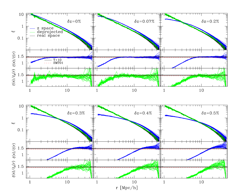
Figure 1: The impact of redshift errors on the measured real- and redshift-space (angle-averaged) correlation functions. The upper sections of each panel show the real-space true correlation functions $\xi(r)$ (black curves), the redshift-space correlation functions $\xi(s)$ (blue curves) and the real-space correlation functions obtained from deprojection, $\xi_{D}(r)$ (green curves). Each line shows the correlation measured in one of the 27 independent sub-boxes (see Section 2). The central and middle sections of each panel show the ratios $\xi(s)/\xi(r)$ and $\xi(s)/\xi_{D}(r)$, respectively. Linear theory predictions of Tinker et al. (2010) and Sheth et al. (2001) are indicated by black solid and red dotted lines, respectively. The grey horizontal bands represent $10\%$ theoretical uncertainties. The panels refer to different redshift errors, as indicated by the labels.

In absence of peculiar velocities, isotropy in galaxy clustering guarantees that iso-correlation contours are circles in the $(r_{\perp},r_{\parallel})$ plane if pair separations are estimated assuming the correct geometry. In this sense, $\xi(r_{\perp},r_{\parallel})$ can be considered a standard circle in much the same way as BAO and Supernovae are considered standard rulers and standard candles, respectively. The choice of an incorrect cosmology will distort these circles in a way that we can accurately predict. Indeed, the relation between comoving separations in two different geometries reads:

$$r_{\perp 1}=\frac{D_{\rm A,1}(z)}{D_{\rm A,2}(z)}r_{\perp 2};\;\;r_{\parallel 1}=\frac{H_{2}(z)}{H_{1}(z)}r_{\parallel 2}\;,$$ (17)

where the subscripts $1$ and $2$ refer to the two cosmological models and $D_{\rm A}$ is the angular diameter distance:

$$D_{\rm A}(z)=\frac{c}{H_{0}(1+z)\sqrt{-\Omega_{\rm k}}}\sin\left(\sqrt{-\Omega_{\rm k}}D_{\rm C}(z)\right)\;.$$ (18)

These relations can be adopted to perform the AP test using the two-point correlation function as follows. In the quest for $\beta$, the choice of a background cosmology is made twice: first to estimate $\xi(s_{\perp},s_{\parallel})$ from observed redshifts and angular positions and then to model $\xi(s_{\perp},s_{\parallel})$ . We shall call assumed and test cosmology the two cosmological models assumed to measure and model $\xi(s_{\perp},s_{\parallel})$ , respectively. The test is performed by computing $\xi_{\rm a}(s_{\perp}^{a},s_{\parallel}^{a})$ for a given assumed cosmology and comparing it with the model $\xi_{\rm t}(s_{\perp}^{t},s_{\parallel}^{t})$ estimated for a test cosmology and rescaled to the assumed one (Eq. (17)):

$$\xi_{\rm a}(s_{\perp},s_{\parallel})=\xi_{\rm t}\left(\frac{D_{\rm A,t}}{D_{\rm A,a}}s_{\perp},\frac{H_{\rm a}}{H_{\rm t}}s_{\parallel}\right)\;.$$ (19)

The correct values of $\beta$, $D_{\rm A}$ and $H$ are found when $\xi_{\rm t}(s_{\perp}^{t},s_{\parallel}^{t})=\xi_{\rm a}(s_{\perp}^{a},s_{\parallel}^{a})$, within the errors. Unfortunately, the small amplitude of GD with respect to RSD and inaccuracies in modelling the latter make results obtained through this procedure not very robust. Moreover, this method depends explicitly on the bias model assumed to derive the DM correlation function from the observed galaxy positions. In this work, we have developed an alternative procedure, described in Section 4, that exploits both RSD and GD directly, and does not require modelling the shape of the DM correlation function and bias.

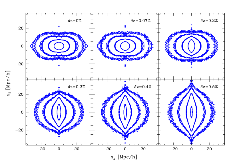
Figure 2: Iso-correlation contours of $\xi(s_{\perp},s_{\parallel})$ measured in the 27 mock catalogues. Contours are drawn in correspondence of the correlation levels $\xi(s_{\perp},s_{\parallel})$ $=\{0.1,\,0.2,\,0.5,\,1.5\}$. Different panels refer to different amplitudes of the redshift errors, as indicated in the labels.

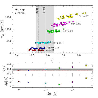
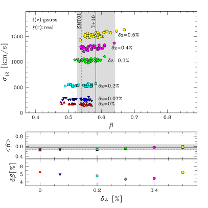
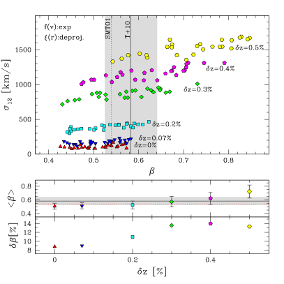
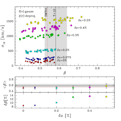
Figure 3: Large upper panels: best-fit parameters $\beta$ and $\sigma_{12}$, as a function of the redshift error $\delta z$. Small bottom panels: systematic and statistical errors, as a function of $\delta z$. Specifically, the upper half windows show the best-fit values of $\beta$, averaged over the 27 mocks, and their scatter, $\sigma(\beta)$, represented by the error bars. The lower half windows show the random component of the relative error, $\sigma(\beta)/\beta\,[\%]$. Black solid and red dotted lines represent theoretical expectations from Tinker et al. (2010) and Sheth et al. (2001), respectively. The grey bands represent a theoretical uncertainty of $10\%$. The assumption on the adopted shape of $f(v)$ and on $\xi(r)$ are labeled in the top-left part of the large upper panels. Top-left part of the figure: $f(v)$ exponential form and true $\xi(r)$. Top-right: $f(v)$ Gaussian form and true $\xi(r)$. Bottom-left part of the figure: $f(v)$ exponential form and deprojected $\xi(r)$. Bottom-right: $f(v)$ Gaussian form and deprojected $\xi(r)$.

3 Measuring $\beta$ from RSD

3.1 The impact of redshift errors and deprojection

Random errors in the measured spectroscopic redshifts contaminate the clustering signal at all scales in a way similar to that of random peculiar motions at small scales. So far they have not been considered in the error budget, as local surveys typically had fairly precise redshift measurements errors ($<100$ km s^-1). A careful assessment of their impact is now in order, especially in view of future surveys using different observing techniques. For example, Euclid will be measuring redshifts from single emission lines in slitless spectroscopic observations, with a requirement on the errors of $\sigma_{z}<0.001(1+z)$, which corresponds to $600$ km s^-1 at $z=1$ (Laureijs et al., 2011).

To assess the impact of redshift errors on the estimates of $\beta$, we have perturbed the redshifts of the mock galaxies (Eq. (4)) by adding a Gaussian noise of amplitude $\sigma_{v}=\{0,\,200,\,500,\,1000,\,1250,\,1500\}$ km/s . These values cover a range extending out to errors that get close to (yet not as large as) those from photometric estimates (which in the best cases have $\sigma_{v}\sim 9000(1+z)$ km/s ). In what follows we express these errors as per cent uncertainties $\delta z[\%]=\{0,\,0.07,\,0.2,\,0.3,\,0.4,\,0.5\}$ (Eq. (4)).

To focus on the impact of redshift errors we do not consider GD, i.e. we assume the correct background cosmology. Moreover, we restrict our analysis to the case of Gaussian redshift errors. This is a quite accurate assumption for modelling the redshift errors of typical spectroscopic galaxy surveys (see e.g. Lilly et al., 2009). Furthermore, even in photometric galaxy surveys, it has been demonstrated that the adoption of a Gaussian distribution to simulate the impact of redshift errors represents a reasonable approximation (see e.g. Cunha et al., 2009; Saglia et al., 2012). We do not consider the impact of the so-called catastrophic errors, the ones caused by the misidentification of one or more spectral features, for the following reasons. In the assumption that the catastrophic outliers represent a perfect isotropic population (i.e. if such errors have a flat distribution), their effect is to reduce the amplitude of the correlation function at all scales. So they do not induce additional distortions in galaxy clustering and do not bias the estimate of $\beta$. On the other hand, clustering distortions might be generated by systematic misidentification of spectral features. Their impact on $\beta$ can only be estimated with mock galaxy catalogues, taking into account all observational effects that may vary case by case.

3.1.1 Real- and redshift-space correlation functions

In Fig. 1 we show the redshift-space two-point correlation functions, $\xi(s)$, measured in the 27 mocks (blue curves in the upper part of the six panels) and compare them to the real-space ones, $\xi(r)$ (black curves). Redshift errors suppress the clustering amplitude on progressively large scales, as expected. A first quantitative assessment of this effect can be obtained from the ratio $\xi(s)/\xi(r)$ which, in the linear limit, is simply related to $\beta$:

$$\frac{\xi(s)}{\xi(r)}=1+\frac{2\beta}{3}+\frac{\beta^{2}}{5}\;.$$ (20)

We plot this ratio in the middle part of each panel in Fig. 1 (blue curves). When $\delta z=0$, this ratio is constant for $r\gtrsim 3$ $h^{-1}\,\mbox{Mpc}$ . On these scales, the value of $\beta$ obtained from Eq. (20) is consistent with theoretical expectations of Sheth et al. (2001) and Tinker et al. (2010), represented by the red dotted and black solid horizontal lines, respectively. The horizontal grey band is plotted for reference and represents a theoretical uncertainty of $10\%$. Increasing redshift errors to $\delta z\sim 0.2\%$ has the effect of suppressing the clustering amplitude on ever larger scales and reduces the range useful to measure $\beta$ but does not bias its estimate. For $\delta z\gtrsim 0.3\%$ the ratio $\xi(s)/\xi(r)$ is biased high in the ever shrinking range of scales in which this ratio is constant, hence inducing a systematic error on $\beta$ obtained from Eq. (20).

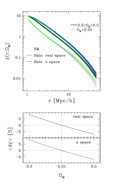
Figure 4: Upper panel: effect of GD on the halo correlation function in real- (middle set of black curves) and redshift-space (upper set of blue curves). The curves in each set have been obtained varying $\Omega_{\rm M}$ in the range $0.2\leq\Omega_{\rm M}\leq 0.3$ (from top to bottom). The lower set of grey curves shows the DM correlation function computed with CAMB (Lewis & Bridle, 2002). The central green lines refer to the choice of the correct value $\Omega_{\rm M}=0.25$. Lower panel: mean fractional error on the estimated $\xi$ as a function of $\Omega_{\rm M}$ in real- and redshift-space.

As a further step towards a realistic estimate of $\beta$, we also assess the impact of the deprojection procedure described in Section 3. The ragged green curves in the upper panels of Fig. 1 show the real-space two-point correlation function obtained from the deprojection procedure, $\xi_{\rm D}$. The corresponding ratio $\xi(s)/\xi_{\rm D}(r)$ is shown in the bottom panels. Interestingly, the deprojected correlation function is in good agreement with the true $\xi(r)$ even for large values of $\delta z$, indicating that the deprojection procedure does not introduce significant systematic errors. However, it increases random errors represented by the scatter among the $\xi(s)/\xi_{\rm D}(r)$ curves.

3.1.2 $\beta$ from the full fit of $\xi(s_{\perp},s_{\parallel})$ 

A better estimate of $\beta$ can be obtained by comparing the measured $\xi(s_{\perp},s_{\parallel})$ with the model described in Section 3. The iso-correlation contours of $\xi(s_{\perp},s_{\parallel})$ calculated in the 27 mocks are shown in Fig. 2 for different values of $\delta z$, indicated in the panels. Contours refer to the iso-correlation levels $\xi(s_{\perp},s_{\parallel})$ $=\{0.1,\,0.2,\,0.5,\,1.5\}$. The effect of increasing redshift errors can be clearly appreciated. The case of no errors ($\delta z=0$) is characterized by the expected squashing of the contours at large separations induced by coherent motions whereas on small scales the fingers-of-God elongation is hardly visible. As already pointed out, this is due to the lack of substructures in the DM haloes, such that the velocity field within virialized structures is poorly sampled. When redshift errors are turned on, fingers-of-God distortions appear and dominate the distortion pattern out to a scale that increases with $\delta z$.

Comparing the correlation function “observed” from the mocks in Fig. 2 with the model presented in Section 2.2, constrains the free parameters $\beta$ and $\sigma_{12}$. This is done by minimizing the standard $\chi^{2}$ function:

$$\chi^{2}=\sum_{i,j}\frac{\left(y_{ij}-y_{ij}^{M}\right)^{2}}{\delta_{ij}^{2}}\;,$$ (21)

where $y_{ij}=\xi(s_{\perp,i},s_{\parallel,j})$ and $y_{ij}^{M}=\xi^{M}(s_{\perp,i},s_{\parallel,j};\beta,\sigma_{12})$ are the measured and model correlation functions, respectively, and $\delta_{ij}=\delta\xi(s_{\perp,i},s_{\parallel,j})$ is the statistical Poisson noise estimated following Mo et al. (1992). In each of the 27 mock catalogues, we fitted over the range $3<r_{\perp},r_{\parallel}<35$ $h^{-1}\,\mbox{Mpc}$ , with linear bins of $1$ $h^{-1}\,\mbox{Mpc}$ both in the parallel and perpendicular directions. As we have explicitly verified, the results presented in this paper do not depend on the particular form of Eq. (21) and on the definition of clustering uncertainties $\delta\xi(s_{\perp},s_{\parallel})$ (for a more detailed discussion see Bianchi et al., 2012).

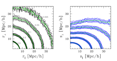
Figure 5: Iso-correlation contours for $\xi(r_{\perp},r_{\parallel})$ (left panel) and $\xi(s_{\perp},s_{\parallel})$ (right panel). Contours are drawn at the iso-correlation levels $\{0.025,\,0.05,\,0.1,\,0.2,\,0.5\}$ indicated by the labels. Different contours drawn at the same correlation level refer to the different values of $\Omega_{\rm M}$ considered. The green contours refer to the correct cosmological model, $\Omega_{\rm M}$ =0.25.

The results are summarized in Fig. 3. Let us focus on the upper left part of the figure. The points in the top panel represent the best-fit values of $\beta$ and $\sigma_{12}$ obtained from each mock catalogue. The different symbols and colours indicate different redshift errors $\delta z$, as specified in the labels. The best-fit $\beta$ values should be compared with theoretical expectations using the Tinker et al. (2010) model (black solid vertical line), which, as discussed previously, is a very good description of the intrinsic linear bias of our simulated haloes. The Sheth et al. (2001) model (red dotted vertical line) is shown for comparison. The vertical grey band shows the $10\%$ uncertainty interval. These results have been obtained by comparing data with a model in which we have used an exponential form for $f(v)$ and the true $\xi(r)$ of the DM haloes in the N-body simulation. Systematic and statistical errors and their dependence on $\delta z$ are quantified in the bottom panel. In the upper part we show the mean value of the best-fit $\beta$ obtained by averaging over the 27 mock catalogues and its scatter, $\sigma(\beta)$, represented by the error bars. In the bottom panel we show the random component of the relative error $\sigma(\beta)/\beta\,[\%]$.

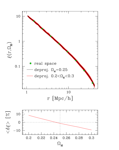
Figure 6: Upper panel: true correlation function in real-space (green dots), deprojected correlation function with $\Omega_{\rm M}$ =0.25 (black curve) and deprojected correlation function with other values of $\Omega_{\rm M}$ (red curves). Bottom panel: mean fractional error $<\delta\xi>$ as a function of $\Omega_{\rm M}$ .

As shown in Bianchi et al. (2012), such systematic error depends on the minimum mass (i.e. the bias) of the haloes considered and tends to decrease up to masses of $10^{13}\mbox{M}_{\odot}$. In Fig. 3 we see, however, that redshift errors larger than $\delta z\sim 0.3\%$ produce an opposite effect, which cancels and then overcomes the intrinsic negative systematic bias on $\beta$. Interestingly, the rms error remains instead substantially constant, when the real-space correlation function is well known (upper panel, $\sim 5\%$ for the volumes considered here).

The upper right part of the same figure shows the results obtained when we model the velocity distribution function $f(v)$ with a Gaussian function instead of an exponential one. The main effect is a very significant reduction of the systematic errors. This is due to the fact that redshift errors, modelled as Gaussian variables, can be regarded as a random velocity field with a distribution function that obeys a Gaussian statistics. What we learn here is that when redshift errors dominate over the pairwise velocity dispersions, then $f(v)$ is best modelled by a Gaussian function with dispersion comparable to $\delta z$. This is demonstrated by the fact that, in the plot, the best-fit values of $\sigma_{12}$ are comparable to the amplitude of the input redshift errors when $\delta z$ is large.

The plots in the bottom part of Fig. 3 are analogous to those shown in the upper half except for the fact that, in this case, we are considering the more realistic scenario in which $\xi(r)$ is not known a priori but obtained from deprojection. Uncertainties in the deprojection procedure increase random errors by a factor of 2-3, depending on the amplitude of $\delta z$.

3.2 The impact of geometric distortions

Before looking in more details into how GD arising from the choice of a wrong cosmological background can actually be exploited to our benefit, we would like first to understand how they impact the measurements of the growth rate from RSD. We first investigate how GD affect the estimate of the correlation function and galaxy bias. We then focus on the measurement of $\beta$. Specifically, we assume a flat cosmology (so that $\Omega_{\Lambda}=1-$$\Omega_{\rm M}$ ) and investigate the effect of choosing an incorrect value of $\Omega_{\rm M}$ in the range $[0.2,0.3]$, in steps of $\Delta\Omega_{\rm M}=0.01$. All the other cosmological parameters are kept fixed to their true values. For this set of experiments we set redshift errors $\delta z=0$. Since the amplitude of GD is smaller than that of RSD, to appreciate their impact we need to minimize sampling errors, i.e. trace velocities and density fluctuations with as many haloes as possible. Thus, in the following we shall use the whole simulation box with all its haloes, instead of the 27 subsamples.

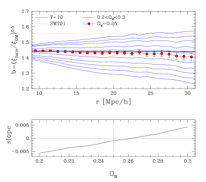
Figure 7: Upper panel: bias of the DM haloes in the simulation, $b=(\xi_{\rm halo}/\xi_{\rm DM})^{0.5}$, as a function of separation, estimated for different values of $\Omega_{\rm M}$ in the range $0.2\leq\Omega_{\rm M}\leq 0.3$ (blue curves). Red dots highlight the case of a correct $\Omega_{\rm M}=0.25$. Error bars represent statistical uncertainties (Mo et al., 1992). Expected values from the models of Tinker et al. (2010) and Sheth et al. (2001) are represented by the horizontal lines. Bottom panel: mean slope of $b(r)$ in the range $10<r<30$ $h^{-1}\,\mbox{Mpc}$ .

3.2.1 Impact on the measured correlation function

Fig. 4 shows the effect of GD on the measured two-point halo correlation function in real- (middle set of black curves) and redshift-space (upper set of blue curves). The lower set of grey curves represents the correlation function of the DM obtained by Fourier transforming the matter power spectrum computed with CAMB (Lewis & Bridle, 2002), which exploits the HALOFIT routine (Smith et al., 2003). In each set, the central, green curve refers to the correct choice of background cosmology, $\Omega_{\rm M}$ =0.25. The other curves refer to $\Omega_{\rm M}$ values ranging from 0.2 (top) to 0.3 (bottom). The choice of the incorrect cosmology also distorts the shape of the computational box. To account for this spurious effect, the random objects used to compute $\xi(r)$ have been generated within the same, distorted volume.

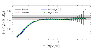
Figure 8: Plot of the ratio between the redshift- and real-space correlation functions, computed from the simulation box after converting redshifts into distances using 10 different cosmologies, corresponding to 10 values of $\Omega_{\rm M}$ in the range $[0.2,0.3]$ (blue curves). The green dots mark the correct value, for $\Omega_{\rm M}$ =0.25, whereas the horizontal lines show theoretical predictions from Tinker et al. (2010) (black solid) and Sheth et al. (2001) (red dotted). The grey band represents a $10\%$ uncertainty around the Tinker et al. value.

GD enhance/dilute the correlation signal on all scales and thus modify the amplitude but not the shape of the correlation function. The effect, quantified by the width of each set of curves, is very small. It can be better appreciated in the bottom panel in which we plot the mean fractional residual of $\xi$, $<\delta\xi>[\%]=\left<(\xi(\Omega_{\rm M})-\xi(\Omega_{\rm M}=0.25)/\xi(\Omega_{\rm M}=0.25)\right>$, where the average is over the interval $1<r<50$ $h^{-1}\,\mbox{Mpc}$ . Since to first-order GD do not modify the shape of $\xi(r)$, the value of $<\delta\xi>$ quantifies the amplitude of the spurious boost in the correlation signal induced by GD. In correspondence to the values $\Omega_{\rm M}$ =0.2 and 0.3, already almost excluded by current observational constraints, the boost is $\sim 8\%$.

Fig. 5 shows the effect of GD on $\xi(r_{\perp},r_{\parallel})$ (left panel) and $\xi(s_{\perp},s_{\parallel})$ (right panel). Contours are drawn at the correlation values $\{0.025,\,0.05,\,0.1,\,0.2,\,0.5\}$. The different curves at a given correlation level refer to different values of $\Omega_{\rm M}$ . The green contours refer to the true geometry.

Fig. 6 demonstrates that GD have little impact on the deprojection procedure. The green dots show the true correlation function in real-space. The black curve shows the deprojected correlation function obtained assuming the correct value of $\Omega_{\rm M}$ . The other red curves refer to the other choices of $\Omega_{\rm M}$ . The effect is the same as in Fig. 4: an incorrect value for $\Omega_{\rm M}$ boosts up or down the correlation amplitude on all scales by a factor $\lesssim 10\%$ (bottom panel), similarly to when $\xi(r)$ is measured directly.

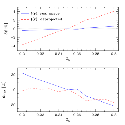
Figure 9: Per cent mismatch between the value of $\beta$ (upper panel) and $\sigma_{12}$ (lower panel) computed for different values of $\Omega_{\rm M}$ and the one obtained assuming the correct $\Omega_{\rm M}$ : $\delta X=[X(\Omega_{\rm M})-X(\Omega_{\rm M}=0.25)]/X(\Omega_{\rm M}=0.25)$, where X can be either $\beta$ or $\sigma_{12}$. The curves show the result obtained assuming the true $\xi(r)$ (solid, blue) or the deprojected one (dashed, red).

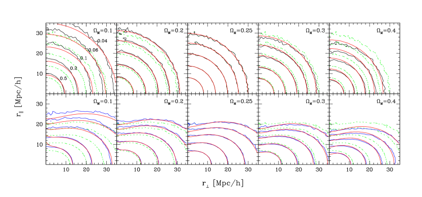
Figure 10: Contour plots of the DM halo correlation function, $\xi(r_{\perp},r_{\parallel})$ (blue curves), in real (top panels) and redshift space (bottom panels), measured for $\Omega_{\rm M}=\{0.1,0.2,0.25,0.3,0.4\}$. The iso-correlation contours correspond to $\xi(r_{\perp},r_{\parallel})$ $=\{0.04,\,0.06,\,0.1,\,0.2,\,0.5\}$. The red lines in both sets of panels correspond to the model $\xi(s_{\perp},s_{\parallel})$ . In the top panels, they simply give the dynamically-undistorted real-space $\xi(r)$ computed for the given cosmology and replicated over $\pi/2$; in the bottom ones, they also include the RSD dispersion model (Eq. (11)) for the best-fit values of $\beta$ and $\sigma_{12}$ derived for that specific $\Omega_{\rm M}$ . The green dotted curves show the geometrically undistorted $\xi(r_{\perp},r_{\parallel})$ measured at the true cosmology ($\Omega_{\rm M}=0.25$), for comparison.

3.2.2 Impact on the measured galaxy bias

An interesting aspect of GD is that the two-point correlation function estimated assuming an incorrect value $\widetilde{\Omega}_{\rm M}$ is different from the correct two-point correlation function measured in a universe with $\widetilde{\Omega}_{\rm M}$. This fact has some practical consequences, for example in the measurement of galaxy bias. Estimates of galaxy bias can be obtained from the ratio of the galaxy and mass two-point correlation functions. For example, the bias of the haloes can be estimated as $b_{\rm halo}(r)=(\xi_{\rm halo}(r,\Omega_{\rm M})/\xi_{\rm DM}(r,\Omega_{\rm M}))^{0.5}$, where $\xi_{\rm halo}(r,\Omega_{\rm M})$ is the real-space halo correlation function measured assuming some value of $\Omega_{\rm M}$ and $\xi_{\rm DM}(r,\Omega_{\rm M})$ is the mass correlation function in the same cosmology. We have computed $b_{\rm halo}(r)$ for the haloes in our mock catalogues. Results are shown in the upper panel of Fig. 7, in which we show $b_{\rm halo}(r)$ obtained for different values of $\Omega_{\rm M}$ in the range $0.2\leq\Omega_{\rm M}\leq 0.3$ (blue curves, from bottom to top). Red dots refer to the correct cosmology and error bars represent 1$\sigma$ statistical uncertainties computed as in Mo et al. (1992). Horizontal lines show the model predictions of Tinker et al. (2010) and Sheth et al. (2001).

These results show that GD affect both the amplitude of the estimated bias and its scale dependence. To estimate the effect, we fit each curve in the plot with a power law function $b(r)=A+\gamma\cdot r$. The spurious scale dependence is quantified by the slope $\gamma$ that we plot in the bottom panel as a function of $\Omega_{\rm M}$ . Ideally, it would seem possible to estimate $\Omega_{\rm M}$ by requiring that $b(r)$ remains flat on those scales where it should be constant. However, the smallness of the effect and the theoretical uncertainties on galaxy bias prevent this technique to be applied to real data.

3.2.3 Impact on the measured value of $\beta$

To assess the GD impact on $\beta$, we have repeated the same analyses presented in Section 3, i.e. we have estimated $\beta$ from the ratio $\xi(s)/\xi(r)$ and by fitting the full $\xi(s_{\perp},s_{\parallel})$ . The blue curves in Fig. 8 show the ratio between the real- and redshift-space correlation functions for 10 different values of $\Omega_{\rm M}$ in the range $0.2\leq\Omega_{\rm M}\leq 0.3$ (from bottom to top). The green dots refer to the true cosmology case. Error bars show the statistical errors computed according to the Mo et al. (1992) prescription. Reference values according to Tinker et al. (2010) and Sheth et al. (2001) are shown by the black solid and the red dotted lines, respectively, with a $10\%$ theoretical uncertainty indicated by the grey band. The scatter among the blue curves is significantly smaller than theoretical uncertainties, thus indicating that estimates of $\beta$ from RSD in the range $3<r[h^{-1}\,\mbox{Mpc}]<50$ are robust to the choice of $\Omega_{\rm M}$ .

The alternative way to estimate $\beta$ from $\xi(s_{\perp},s_{\parallel})$ confirms this result. Fig. 9 quantifies the amplitude of the effect. In the upper panel we show the per cent difference between $\beta$ computed for a given $\Omega_{\rm M}$ , indicated on the X-axis, and the one obtained assuming the correct model $\Omega_{\rm M}$ =0.25. The solid blue curve refers to the case in which we model $\xi(s_{\perp},s_{\parallel})$ using the true $\xi(r)$, whereas the red dashed curve shows the case in which $\xi(r)$ has been obtained by deprojecting $\xi(s_{\perp},s_{\parallel})$ . In both cases, the impact of GD is rather small, especially if compared to that of redshift errors. The corresponding error induced on $\beta$ is less than $1\%$ over the whole range of $\Omega_{\rm M}$ analysed, when the true $\xi(r)$ is used in the model. Using the deprojected $\xi(r)$, the maximum error on $\beta$ rises to $\sim 4\%$. Finally, the lower panel shows the impact of GD on the other parameter of the fit, the pairwise dispersion $\sigma_{12}$. The error on this parameter turns out to be larger than the one on $\beta$, rising to $\sim 20\%$ for the extreme values of $\Omega_{\rm M}$ .

4 Disentangling dynamic and geometric distortions

In this section, we investigate the possibility to perform the AP test using $\xi(s_{\perp},s_{\parallel})$ . The goal is to constrain both $\beta$ and the cosmological parameters that enter Eq. (3) exploiting anisotropies in galaxy clustering induced by RSD and GD.

4.1 The method

As we have anticipated in Section 2.3, a common approach is to use Eq. (19) to model the two-point correlation function in a series of test cosmological models and compare it with the measured one (Ballinger et al., 1996). Here we adopt an alternative procedure, which is a generalization of the iterative method introduced in Guzzo et al. (2008) and that is found to be robust. The method consists in repeating the measurement of the correlation function in different test cosmologies, and then modelling only its RSD. Our working hypothesis is that, by construction, the agreement between model and data will be maximum when the test cosmology coincides with the true cosmology of the Universe, i.e. without GD.

The steps of the procedure can be summarized as follows.

1. Choose a cosmological model to convert angular positions and redshifts into comoving coordinates.

2. Measure $\xi(s_{\perp},s_{\parallel})$ .

3. Estimate the real-space correlation function, $\xi(r)$, required to model dynamic distortions (e.g. through the deprojection technique).

4. Model only dynamic distortions (e.g. through Eq. 11), and derive the best-fit values of $\beta$ and $\sigma_{12}$ that minimize the $\chi^{2}$ function given by eq. 21.

5. Save this specific minimum value of the $\chi^{2}$, that we shall call $F(\{D_{\rm A},H\}_{i})$.

6. Go back to point (i) using a different test cosmology and estimate a new value for $F$.

Once the whole set of $\{D_{\rm A},H\}_{i}$ has been explored, the “best of the best” set of parameter values $(\beta,\sigma_{12},D_{\rm A},H)$ will be then identified by the minimum value of $F(\{D_{\rm A},H\}_{i})$. The main differences between this procedure and the usual one are that i) the observed and model correlation functions assume the same test cosmological model, and ii) once $D_{\rm A}$ and $H$ are fixed, one only needs to model RSD. In the case of a flat $\Lambda$CDM background, the success of this strategy is guaranteed by the small covariance between $\Omega_{\rm M}$ and $\beta$ (see e.g. Ross et al., 2007). As a consequence, one can obtain an unbiased estimate of $\Omega_{\rm M}$ even for an incorrect choice of $\beta$ and $\sigma_{12}$.

One advantage of our procedure is that it does not require the modelling of the galaxy bias. Since tha galaxy correlation function can be obtained directly from the data through the deprojection technique, it is not necessary to model the shape of the DM correlation function (at point (iii)). The only assumption of the method is the intrinsic isotropy of the clustering.

One disadvantage is the computational cost, since one has to estimate $\xi(s_{\perp},s_{\parallel})$ for each cosmological model to test. However, the use of optimized linked-list-, Tree- and FFT-based algorithms allows $\xi(s_{\perp},s_{\parallel})$ to be computed sufficiently fast, as to efficiently explore the parameter space without resorting to supercomputing facilities. Alternatively, instead of directly measuring the correlation function at different test cosmologies, it is actually sufficient to measure $\xi(s_{\perp},s_{\parallel})$ in a fiducial cosmology and rescale the result to a test cosmology, using Eq. (19). A second disadvantage is related to the estimate of the errors. The best-fit parameters are found by minimizing a function $F$ that does not obey a $\chi^{2}$ statistics. The reason is that the data themselves, which in this case coincide with the measured $\xi(s_{\perp},s_{\parallel})$ , depend on $D_{\rm A}$ and $H$. Therefore, since the values of $F$ evaluated at different $D_{\rm A}$ and $H$ do not refer to the same dataset, the function $F$ does not follow a $\chi^{2}$ statistics. As a consequence, errors on $D_{\rm A}$ and $H$ have to be evaluated in a different way, as we shall see below.

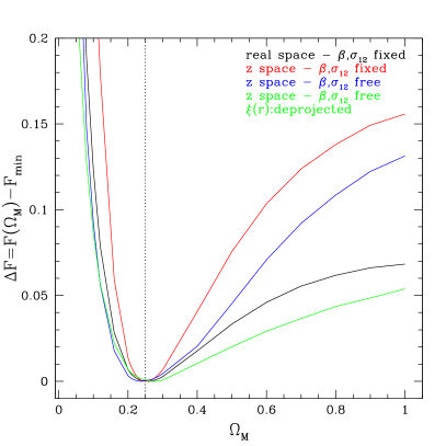
Figure 11: The “pseudo-likelihood” function $\Delta F$ as a function of $\Omega_{\rm M}$ , obtained with the method described in Section 4.2. i) In real-space fixing $\beta=\sigma_{12}=0$ (black line). ii) In redshift-space, but fixing $\beta$ and $\sigma_{12}$ to their best-fit values as derived with the correct cosmology (red line). iii) Same, but leaving also $\beta$ and $\sigma_{12}$ as free parameters, either assuming perfect knowledge of the true real-space $\xi(r)$ (blue line) or iv) recovering it through deprojection (green line).

4.2 Joint constraints on $\Omega_{\rm M}$ and $\beta$

We start our analysis considering the case of a flat $\Lambda$CDM model in which $\Omega_{\rm M}$ , the mass density parameter, fully characterizes the expansion history and geometry of the Universe. Fig. 10 illustrates the result of applying this procedure to the full catalogue of DM haloes. The different panels show the iso-correlation contours of the two-point correlation function measured in real- (black curves in the top panels) and redshift-space (blue curves in the bottom panels). Contours are drawn at the correlation levels $\{0.04,\,0.06,\,0.1,\,0.2,\,0.5\}$. Different panels refer to the different values of $\Omega_{\rm M}$ used to compute distances and estimate the correlation function, as indicated by the labels. The green dotted curves are drawn for reference and show the predictions for the true cosmological model $\Omega_{\rm M}$ =0.25. As such, in the central panel they coincide with the black and blue curves. The red curves show the corresponding model for the two-point correlation function obtained using the best-fit values of $\beta$ and $\sigma_{12}$ estimated at each value of $\Omega_{\rm M}$ .

In real-space (top panels) the model for $\xi(r_{\perp},r_{\parallel})$ is simply a replica over all angles of the real-space correlation function $\xi(r)$ (i.e. no RSD are present, corresponding to setting $\beta=\sigma_{12}=0$ in the dispersion model). This is shown here to evidence the interplay of the two effects. It could be seen as an idealized case in which we are able to perfectly correct for RSD, or can hypothetically reconstruct the real-space galaxy distribution. The iso-correlation contours are thus circles in the $(r_{\perp},r_{\parallel})$ plane, when the correct cosmology is used. The effect of GD when varying the cosmology is then quantified by the mismatch between the green and the black contours. As evident, the best-fit value for $\Omega_{\rm M}$ can be found by minimizing the difference between the red and the black curves, which is in practice the AP test. The best agreement is found for $\Omega_{\rm M}$ =0.25, as expected, showing that this procedure is unbiased.

Similar considerations can still be applied to the redshift-space case (bottom panels). For a given $\Omega_{\rm M}$ , the amplitude of the mismatch is similar to that found in real-space. This fact validates the hypothesis that GD and RSD are substantially independent. The difference between red and blue curves is still minimized for the correct reference value, $\Omega_{\rm M}$ =0.25, showing that the result is unbiased also in redshift-space.

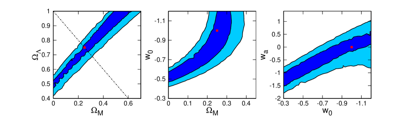
Figure 12: The 68 and 95 per cent pseudo-likelihood probability contours in the $\Omega_{\rm M}-\Omega_{\Lambda}$ (left panel), $\Omega_{\rm M}-w_{0}$ (central panel) and $w_{0}-w_{a}$ (right panel) planes. In each case, the other two parameters not shown are fixed to their true values. These constraints have been obtained in redshift-space, using the true $\xi(r)$ and fixing $\beta$ and $\sigma_{12}$ to their best-fit values as derived with the correct cosmology. The red squares mark the correct cosmological parameters of the simulation. The dotted black line in the left panel shows the flat background case: $\Omega_{\Lambda}=1-\Omega_{\rm M}$.

Let us then quantify the ability of the proposed technique to jointly estimate $\Omega_{\rm M}$ and $\beta$. As we described, the best-fit values for $(\beta,\sigma_{12},\Omega_{\rm M})$ are found at the minimum of the pseudo–$\chi^{2}$ function, $F$. Note that, in this procedure, both the model and the measured $\xi(s_{\perp},s_{\parallel})$ depend on $\Omega_{\rm M}$ . The same happens with the errors, since the number of pairs in each bin is modified by the presence of GD. However, we have verified that this effect is small and can be ignored. More specifically, the shape of the function $F$ and the position of its minimum are very insensitive to $\delta\xi(\Omega_{\rm M})$. In Fig. 11 we plot $\Delta F=F(\Omega_{\rm M})-F_{\rm min}$, where $F_{\rm min}$ is the minimum value of $F$ found during the exploration of the cosmological parameter grid ($\Omega_{\rm M}$ _i in our case). As in Section 3, we fit over the range $3<r_{\perp},r_{\parallel}<35$ $h^{-1}\,\mbox{Mpc}$ , with linear bins of $1$ $h^{-1}\,\mbox{Mpc}$ both in the parallel and perpendicular directions.

To evidence how the technique operates in detail, and understand its possible limitations, we proceed in increasing steps, as we did in Fig. 10. We therefore first test the validity of the best-fitting procedure in real-space, an ideal case that would correspond to a perfect subtraction (or absence) of RSD. In this case, the value of $F$ quantifies the mismatch between the black and the red contours shown in the top panels of Fig. 10. The corresponding function $\Delta F$ is represented by the black curve in Fig. 11. The minimum of the curve is found for $\Omega_{\rm M}$ = 0.25, again showing that the fitting procedure gives unbiased results.

The red curve refers to redshift-space. It shows the values of $\Delta F$ obtained as a function of $\Omega_{\rm M}$ _i, after fixing $\beta$ and $\sigma_{12}$ to the best-fit values computed at $\Omega_{\rm M}=0.25$. In practice, this is again an idealized case in which the correct distortion pattern is known a priori and used as a reference against the one observed when assuming different cosmologies. The RSD model is, in other words, inaccurate for all choices of $\Omega_{\rm M}$ but for $\Omega_{\rm M}=0.25$. Also in this case, the minimum of $\Delta F$ is found for $\Omega_{\rm M}=0.25$, thus indicating that the switch-on of RSD does not bias our estimate. Interestingly, in this case the minimum is sharper than in the real-space case (black curve); this can be explained as due to the stronger constraints posed by the RSD pattern in the observed $\xi(r_{\perp},r_{\parallel})$ , which reduces simmetry with respect to the simple real-space case. In other words, this is telling us that, if we were able to know redshift distortions perfectly, e.g. from an independent measurement, then the constraints on the background cosmological parameters from an AP test would be more precise than those expected from the standard real-space geometric test. This is shown in this simplified case by the fact that the red curve yields a smaller uncertainty on $\Omega_{\rm M}$ than the black one.

In the general case, however, we do not know a priori the amount of redshift distortions and we would rather like to estimate also $\beta$ (and $\sigma_{12}$), together with $\Omega_{\rm M}$ . The resulting constraint is shown by the blue and green curves. For the blue curve, we have assumed perfect knowledge of the real-space correlation function $\xi(r)$ (i.e. we have measured it directly from real-space positions in the simulation). We have already seen how crucial this is, as an ingredient in the RSD model. Also in this case, the minimum is found at the expected value $\Omega_{\rm M}=0.25$, although the fit is less constraining because of the increased degrees of freedom in the model. The green curve, instead, depicts what happens with the same freedom in the model but in the most realistic case when one reconstructs $\xi(r)$ by deprojecting $\xi(s_{\perp},s_{\parallel})$ . Although the estimate of $\Omega_{\rm M}$ is still almost unbiased (i.e. the systematic errors are smaller than the random ones), the minimum is now much shallower, thus indicating lower constraining power, i.e. a larger statistical uncertainty in the recovered value. These errors reflect the uncertainties in the deprojection procedure, which are responsible for the scatter among the green curves in Fig. 1.

As previously discussed, the function $\Delta F$ does not obey a $\chi^{2}$ statistics and therefore we cannot use the curves in Fig. 11 to define confidence interval and estimate errors on $\Omega_{\rm M}$ . Ideally, one should repeat the analysis using many halo catalogues extracted from the simulation. However, in our analysis we have already considered the whole computational box and would need to run more, independent N-body simulations, which are not available. We are therefore forced to evaluate errors using techniques that are typical of error estimates from observational samples. Specifically, we use the “block-wise bootstrap” technique: we divide the box into 27 independent sub-boxes and build several boostrap samples, each containing 27 sub-samples selected at random, with replacement, from the original dataset. The 1-$\sigma$ errors are then evaluated from the scatter on the relevant quantities among the bootstrap samples (Norberg et al., 2009).

We apply this technique to quantify the uncertainties on our estimated values of $\Omega_{\rm M}$ , $\beta$ and $\sigma_{12}$ when using the procedure described in this section as applied in a realistic situation, i.e. redshift-space with free parameters (i.e. the cases of the blue and green curves in Fig. 10). We obtain a value $\Omega_{\rm M}$ =$0.24\pm 0.03$, corresponding to a 1-$\sigma$ uncertainty of $12\%$, when the true $\xi(r)$ is used in the RSD model (i.e. the black curve). When using the deprojected $\xi(r)$, the error on $\Omega_{\rm M}$ grows up to $\sim 40\%$. Still, no systematic bias is apparent.

Finally, all these results have been obtained assuming no errors on measured redshifts. We checked directly that the impact of these errors on our conclusions is indeed negligible, as long as $\delta z\lesssim 0.2\%$. However, when $\delta z>0.3\%$, the resulting systematic errors on $\beta$ do propagate to $\Omega_{\rm M}$ and can bias its estimate.

4.3 Constraints on curvature and on the DE equation of state

In this section, we investigate how GD can help in detecting possible deviations from a flat $\Lambda$CDM scenario. Let us assume a more general DE model with equation of state:

$$\frac{p_{\rm DE}}{\rho_{\rm DE}}=w_{0}+w_{a}\frac{z}{1+z}\;,$$ (22)

(Chevallier & Polarski, 2001; Linder, 2003). In this case, the relevant cosmological parameters are: $\Omega_{\rm M}$ , $\Omega_{\Lambda}$, $w_{0}$ and $w_{a}$ (see Eqs. 3–18–19).

As described in the previous sections, our AP test exploits only clustering distortions and does not consider the information encoded in the shape of the correlation function. The advantage is that our method does not depend on the galaxy bias model. The drawback is that with no constraints on the shape of $\xi(r)$, the above parameters are degenerate. This can be seen in Fig 12, that shows the $68$ and $95$ per cent pseudo-likelihood probability contours in the $\Omega_{\rm M}-\Omega_{\Lambda}$, $\Omega_{\rm M}-w_{0}$ and $w_{0}-w_{a}$ planes. In each plot, the other two parameters that are not shown are fixed to the true values. The red squares mark the cosmological parameters of the simulation. These constraints have been obtained in redshift-space, using the true $\xi(r)$ and fixing $\beta$ and $\sigma_{12}$ to their best-fit values as derived with the correct cosmology, so that the red curve in Fig. 11 corresponds to the pseudo-likelihood contours along the dotted black line in Fig 12, that illustrates the case of a flat universe ($\Omega_{\Lambda}=1-\Omega_{\rm M}$). The flatness constraint is almost perpendicular to the degeneracy in the $\Omega_{\rm M}-\Omega_{\Lambda}$, and is the reason that allowed to constrain $\Omega_{\rm M}$ in the previous section.

5 Discussion and Conclusions

In this work, we have investigated some relevant limitations existing when using the anisotropy of galaxy clustering to measure the growth rate of density fluctuations, while accounting at the same time for the extra distortions induced by the cosmology-dependent mapping of redshifts into distances. More specifically, we have assessed the impact of different types of uncertainties, both observational and theoretical, on the estimated values of $\beta$, the anisotropy parameter closely related to the growth rate. We have then tested how well, in presence of RSD, the correct underlying cosmology can be inferred.

The main results of these analyses can be summarized as follows.

• The impact of Gaussian redshift errors on the estimate of RSD can be assimilated to a generalized small-scale Gaussian velocity dispersion, which can be quantified in terms of a single parameter analogous to the usual pairwise velocity dispersion $\sigma_{12}$.

• In catalogues with volume, density and bias similar to the ones analysed in this work, we can estimate $\beta$ from RSD with an accuracy of $5-10\%$, regardless of the redshift errors. A general scaling formula for the statistical error on $\beta$ as a function of the survey parameters is calibrated and presented in the companion paper by Bianchi et al. (2012).

• With typical spectroscopic redshift errors ($\sigma_{v}\lesssim 600$ km/s ), the anisotropy parameter $\beta$ measured using galaxy-sized haloes is systematically underestimated by $\sim 10\%$. This is discussed in more detail in Bianchi et al. (2012), where it is also shown that this systematic error depends on the bias of the haloes considered.

• Larger redshift errors ($\sigma_{v}\gtrsim 1000$ km/s ) introduce an opposite systematic bias in the estimate of $\beta$, if not modelled properly. This can be partly alleviated using a Gaussian model for the velocity distribution function $f(v)$, rather than the exponential one. Note, however, that this may be influenced by the fact that a Gaussian distribution has been assumed for redshift errors (which is, in any case, a realistic choice for spectroscopic observations).

• A key ingredient in modelling RSD in a sample is a good knowledge of the underlying real-space correlation function $\xi(r)$. Random errors on $\beta$ are increased by a factor $\sim 2$ when $\xi(r)$ is obtained through the deprojection of the observed $\xi(s_{\perp},s_{\parallel})$ , with respect to when using the correct $\xi(r)$.

• GD arising from an incorrect choice of the background cosmology affect both the measured correlation function and its model, and thus can impact the estimate of $\beta$. However, we have seen that this is very small, meaning that the value of $\beta$ can be recovered with similar accuracy even assuming a wrong cosmological model.

• GD have an impact on the estimated galaxy bias. The effect is to introduce a spurious scale dependence in the biasing function on those scales in which it is supposed to be constant. However, the effect is very small and of the same order of theoretical uncertainties in current bias models.

• We have implemented and tested an alternative procedure to perform the Alcock-Paczynski test from the observed $\xi(s_{\perp},s_{\parallel})$ , measuring simultaneously $\beta$ and the parameters that enter Eq. (3). This is based on the (verified) assumptions that the effect of RSD dominates over GD and that the best match between RSD observations and the RSD model is realized for the correct cosmology. We have shown that this procedure is robust and the results unbiased, in the case of a flat $\Lambda$CDM model. We give a first, approximated estimate of the uncertainty that can be expected for $\Omega_{\rm M}$ through a block-wise bootstrap resampling. In a volume $V=2.4\cdot 10^{9}(h^{-1}\,\mbox{Mpc})^{3}$, we find that the expected errors on $\Omega_{\rm M}$ are of the order of $\sim 12\%$, rising up to $\sim 40\%$ if the deprojected $\xi(r)$ is used instead of the true one. The results are very insensitive to the accuracy of the model used to describe RSD and to the magnitude of redshift measurement errors (up to $\delta z\sim 0.2\%$). Finally, we have investigated how GD can be exploited to constrain both the curvature of the Universe and the DE equation of state.

In this paper we focused on the analysis of a simulation snapshot centered at $z=1$. Clearly, we could have analysed a corresponding box at $z=0$, but preferred to focus on a redshift range which is becoming more and more important with ongoing deep surveys like VIPERS (which has an effective redshift around 0.8 and stretches out to $z=1.4$ with its brightest galaxies (Guzzo et al., in preparation)), and with future larger surveys. Also, we concentrated our analysis on intermediate scales, $r<50$$h^{-1}\,\mbox{Mpc}$ , where most of the RSD signal lies. These scales will remain important for these studies also in future surveys in which larger, even more linear scales will be surely better sampled, but nevertheless not sufficient alone for reaching the per cent precisions we are aiming for.

Finally, we also limited our modelling to the simple dispersion model. We are aware, as we show in our companion paper (Bianchi et al., 2012), that this is not a fully appropriate description of clustering and RSD on such mildly non-linear scales, when the precision on statistical errors becomes high. This is very probably at the origin of the observed $\sim 10\%$ systematic error on the recovered $\beta$ and significant work is being performed to improve it (see e.g. de la Torre & Guzzo, 2012, and references therein). Still, in its simplicity the dispersion model performs surprisingly well when compared to much more complicated expressions (e.g. Blake et al., 2011) and delivers statistical errors comparable or smaller than those of more sophysticated non-linear corrections (de la Torre & Guzzo, 2012). The fact that the impact of non-linear effects on estimated errors is quite limited is also suggested by the close similarity of the errors on $\beta$ estimated as in this paper to those predicted by a Fisher matrix analysis (Bianchi et al., 2012).

References

- Acquaviva & Gawiser (2010) Acquaviva V., Gawiser E., 2010, Phys. Rev. D, 82, 082001
- Alcock & Paczynski (1979) Alcock C., Paczynski B., 1979, Nature, 281, 358
- Amendola et al. (2005) Amendola L., Quercellini C., Giallongo E., 2005, Mon. Not. R. Astron. Soc., 357, 429
- Angulo et al. (2008) Angulo R. E., Baugh C. M., Frenk C. S., Lacey C. G., 2008, Mon. Not. R. Astron. Soc., 383, 755
- Ballinger et al. (1996) Ballinger W. E., Peacock J. A., Heavens A. F., 1996, Mon. Not. R. Astron. Soc., 282, 877
- Barkana (2006) Barkana R., 2006, Mon. Not. R. Astron. Soc., 372, 259
- Bianchi et al. (2012) Bianchi D., Guzzo L., Branchini E., Majerotto E., de la Torre S., Marulli F., Moscardini L., Angulo R. E., 2012, ArXiv e-prints
- Blake et al. (2011) Blake C., et al., 2011, Mon. Not. R. Astron. Soc., 1599
- Cabré & Gaztañaga (2009a) Cabré A., Gaztañaga E., 2009a, Mon. Not. R. Astron. Soc., 393, 1183
- Cabré & Gaztañaga (2009b) Cabré A., Gaztañaga E., 2009b, Mon. Not. R. Astron. Soc., 396, 1119
- Carbone et al. (2012) Carbone C., Fedeli C., Moscardini L., Cimatti A., 2012, J. Cosm. Astro-Particle Phys., 3, 23
- Carbone et al. (2011a) Carbone C., Mangilli A., Verde L., 2011a, J. Cosm. Astro-Particle Phys., 9, 28
- Carbone et al. (2011b) Carbone C., Verde L., Wang Y., Cimatti A., 2011b, J. Cosm. Astro-Particle Phys., 3, 30