A 5.5-year robotic optical monitoring of Q0957+561: substructure in a non-local cD galaxy

New light curves of the gravitationally lensed double quasar Q0957+561 in the $gr$ bands during 2008–2010 include densely sampled, sharp intrinsic fluctuations with unprecedentedly high signal-to-noise ratio. These relatively violent flux variations allow us to very accurately measure the $g$-band and $r$-band time delays between the two quasar images A and B. Using correlation functions, we obtain that the two time delays are inconsistent with each other at the 2$\sigma$ level, with the $r$-band delay exceeding the 417-day delay in the $g$ band by about 3 days. We also studied the long-term evolution of the delay-corrected flux ratio $B/A$ from our homogeneous two-band monitoring with the Liverpool Robotic Telescope between 2005 and 2010. This ratio $B/A$ slightly increases in periods of violent activity, which seems to be correlated with the flux level in these periods. The presence of the previously reported dense cloud within the cD lensing galaxy, along the line of sight to the A image, could account for the observed time delay and flux ratio anomalies.

1 Introduction

The optical continuum variability of the gravitationally lensed double quasar Q0957+561 at redshift $z$ = 1.41 has been widely studied since its discovery by Walsh et al. (1979). Several monitoring campaigns focused on the determination of the time delay between the two quasar images A and B (e.g., Vanderriest et al. 1989; Kundić et al. 1997; Serra-Ricart et al. 1999), where a major breakthrough occurred in Kundić et al. (1997), who used Apache Point Observatory (APO) data. The 1.5-year monitoring programme with the APO 3.5 m telescope led to an accurate time delay $\Delta t_{BA}$ = 417 $\pm$ 3 d (2$\sigma$ confidence interval; A leading) in the $g$ band. Kundić et al. (1997) also reported $\Delta t_{BA}\sim$ 420 d in the $r$ band, which was consistent with the $g$-band delay measurement. A recent 2.5-year campaign with the Liverpool 2 m robotic telescope (LRT) has confirmed the APO $g$-band delay, but it has not allowed us to measure a reliable time delay in the $r$ band (Shalyapin et al. 2008, Paper I). Unfortunately, very accurate estimates of multiband delays between Q0957+561A and Q0957+561B remain elusive because of the absence of very prominent flux variations with signal-to-noise ratio $S/N\geq$ 10, where $S/N$ for a given fluctuation is defined as the ratio between its semiamplitude and mean flux error (see Paper I). The strong gravitational lensing scenario predicts the existence of an achromatic delay (e.g., Schneider et al. 1992; Kochanek et al. 2004), while the possible detection of different delays in different optical bands would provide extremely valuable information on the physical properties of the intervening medium.

Using the APO light curves for the two quasar images, Collier (2001) found that the $r$-band main fluctuations lag with respect to those in the $g$-band by 3.4 ${}^{+1.5}_{-1.4}$ d (1$\sigma$ interval). This interband delay was interpreted as clear evidence for stratified reprocessing within an accretion disc that is irradiated by a central high-energy source. The accretion disc would orbit the central supermassive black hole of the quasar. Interestingly, $\Delta t_{rg}\sim$ 4 d for the image B data alone, whereas $\Delta t_{rg}\sim$ 1 d for the image A data alone. These two estimates agreed within the 1$\sigma$ error bars, but the shortest delay from A data was thought to be underestimated as a result of the relatively poor sampling and variability behaviour (Collier 2001). The LRT follow-up of Q0957+561A also led to interband delay estimates centred on 3–4.5 d (Paper I), seemingly supporting the four-day value for both images. We note that the presence of equal interband delays for the two quasar images is equivalent to the occurrence of equal delays between images in different bands.

One can also obtain the delay-corrected flux ratio at time $t$: $B/A=S_{B}(t)/S_{A}(t-\Delta t_{BA})$, where $S_{A}$ and $S_{B}$ are fluxes of Q0957+561A and Q0957+561B, respectively. Although the strong gravitational lensing scenario produces achromatic and stationary flux ratios of lensed quasars (e.g., Schneider et al. 1992; Kochanek et al. 2004), actual scenarios are not so simple. Chromatic flux ratios are usually related to differential extinction (e.g., Falco et al. 1999; Elíasdóttir et al. 2006) or differential microlensing (e.g., Yonehara et al. 2008). In addition, time-variable flux ratios are likely due to differential microlensing by stars in lensing galaxies (e.g., Irwin et al. 1989; Paraficz et al. 2006). The light rays associated with the two images of Q0957+561 pass through two separate regions within the central cluster cD galaxy at $z$ = 0.36 acting as main gravitational lens (Stockton 1980; Young et al. 1980; Garrett et al. 1992). Thus, while the optical continuum of the B image probably does not suffer significant dust extinction, the optical continuum light of the A image is affected by a dense dusty cloud inside the cD galaxy (Goicoechea et al. 2005a, b). This differential extinction produces a chromatic flux ratio, whose $R$-band value was basically constant from 1987 through 2000 (e.g., see Fig. 3 of Oscoz et al. 2002). The LRT observations also support the constancy of $B/A$ over the 2000–2007 period in the $g$ and $r$ bands. Despite the fact that stars in the main lensing galaxy may induce variations in $B/A$ (see above), the time-domain studies of Q0957+561 over two decades failed to detect these variations.

We conducted a long-term photometric monitoring programme of Q0957+561 using the LRT at La Palma, Canary Islands. The observations are part of the Liverpool Quasar Lens Monitoring (LQLM) project (Goicoechea et al. 2010). Two-colour light curves of Q0957+561 during the first phase of this project (LQLM I; from January 2005 to July 2007) were published in Paper I. Here, in Sect. 2, we present new light curves in the $g$ and $r$ bands (LQLM II; from February 2008 to July 2010). These new light curves show densely sampled, sharp intrinsic fluctuations with $S/N\sim$ 10, which are used in Sect. 3 to measure delays with unprecedented accuracy. In Sect. 4, we discuss the time-evolution of $B/A$ over the 2000–2010 decade in the $g$ and $r$ bands. Our main conclusions are included in Sect. 5. In Sect. 6, we briefly comment on some scenarios that could account for the observational results, as well as future prospects.

2 Observations and data reduction

All LQLM II optical frames of Q0957+561 were obtained with RATCam. This is a CCD camera with a $4\aas@@fstack{\prime}6\times 4\aas@@fstack{\prime}6$ field of view, having a pixel scale of $\sim 0\aas@@fstack{\prime\prime}27$ (binning 2$\times$2). To obtain a photometric signal-to-noise ratio of $\sim$ 100 for the two quasar images for each observing night, we set the exposure times to 120 s per night in the $g$ and $r$ bands. Apart from the basic pre-processing tasks included in the LRT pipeline, we cleaned some cosmic rays and interpolated over bad pixels using the bad pixel mask.

The pre-processed frames flow through our photometric pipelines to subsequent stages of processing (e.g., see the flowchart in Figure 1 of Goicoechea et al. 2010). At an initial stage, the crowded-field photometry pipeline produces the instrumental fluxes of the quasar images. The frames that are of little or no interest were then removed from the initial data set. In Paper I we showed that quasar images with signal-to-noise ratio above 80 produce high-quality photometric results. Thus, only $gr$ frames with signal-to-noise ratio $\geq$ 80 over Q0957+561A are passed through the transformation pipeline. This pipeline transforms instrumental magnitudes into SDSS magnitudes, and the calibration-correction scheme is described in Appendix A of Paper I.

For the long-term data in the $g$ and $r$ bands, we used a sophisticated transformation model incorporating zero-point, colour and inhomogeneity terms. Although this last term played an important role when analysing earlier observations with the LRT (2005–2007; Paper I), the new data in the 2008–2010 period indicate that inhomogeneities have been weaker in the most recent years. Some improvements to the telescope in September 2007 seem to have decreased inhomogeneities and typical seeing values. To obtain $g$-SDSS magnitudes of a quasar image, we initially considered an average colour $\langle(g-r)_{SDSS}\rangle$ in its colour correction (see Appendix A of Paper I). However, variations of $(g-r)_{SDSS}$ may introduce a non-negligible colour noise, which should be removed from the brightness record. The amplitude of the colour noises for the two images is $\sim$ 10 mmag, and we eliminated these systematic noises in our 2008–2010 $g$-SDSS records. We also turned magnitudes into fluxes (in mJy) using SDSS conversion equations.

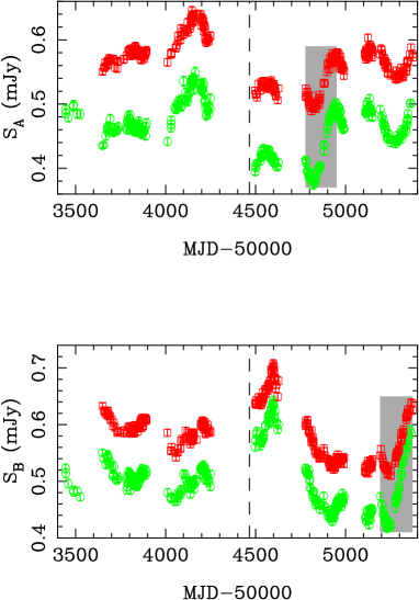
Figure 1: Fluxes of Q0957+561A (top panel) and Q0957+561B (bottom panel) in the $g$ and $r$ bands of the SDSS photometric system. Circles denote the $g$-SDSS light curves and squares represent the $r$-SDSS records. The whole optical data set is separated into two parts by a vertical dashed line: LQLM I (2005–2007) and LQLM II (2008–2010). The new effort in the 2008–2010 period doubles our contribution to the two-colour variability database of Q0957+561. We also highlight the LRT main fluctuations using grey rectangles (see main text).

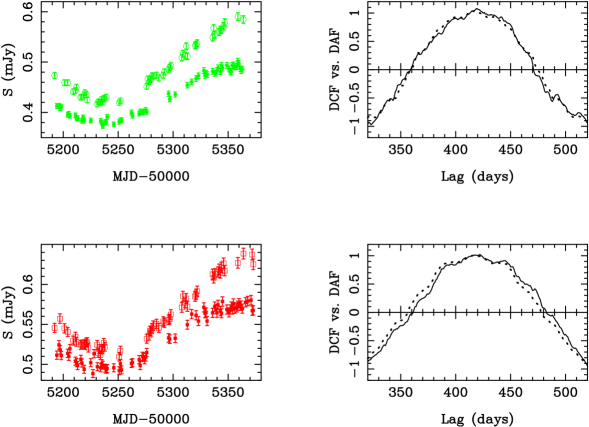
Figure 2: LRT main fluctuations and some of their correlation functions. Top left panel: the fluxes of Q0957+561A (shifted forwards in time in 417 d; filled circles) and Q0957+561B (open circles) in the $g$ band. Top right panel: the AB cross-correlation (solid line), and the average of the AA and BB autocorrelations (shifted by + 417 d; dashed line) in the $g$ band for $\alpha$ = 6 d. Bottom left panel: the fluxes of Q0957+561A (shifted forwards in time in 417 d; filled squares) and Q0957+561B (open squares) in the $r$ band. Bottom right panel: the AB cross-correlation (solid line), and the average of the AA and BB autocorrelations (shifted by + 417 d; dashed line) in the $r$ band for $\alpha$ = 9 d.

A large optical variability database, incorporating previous LQLM I fluxes and the new LQLM II light curves of Q0957+561, is available in tabular format at the CDS: Table 1–2 include 357 $g$-SDSS and 371 $r$-SDSS pairs of fluxes ($S_{A}$,$S_{B}$), respectively. Each of these tables contains the following information. Column 1 lists the observing date (MJD–50 000), Columns 2 and 3 indicate the flux and its error for the image A, and Columns 4 and 5 give the flux and its error for the image B. The LQLM optical light curves of Q0957+561A (top panel) and Q0957+561B (bottom panel) are shown in Fig. 1. A vertical dashed line on 1 January 2008 separates the LQLM I and II periods. In the second monitoring period, there are 215 $g$-SDSS fluxes for each quasar image (circles), as well as 239 $r$-SDSS pairs of fluxes (squares). We achieve 1–1.3% photometric accuracy during the 2008–2010 period. Moreover, excluding the unavoidable seasonal gaps, the average separation between adjacent data is only three days. The new LRT light curves display four densely sampled, very prominent variations (see the two grey highlighted regions in Fig. 1). The two variations in $S_{A}$ are basically repeated in $S_{B}$ 14 months later, which means that these four fluctuations have an intrinsic origin. They also have $S/N\sim$ 10, and can be considered as the LRT main fluctuations.

3 Time delays from the LRT main fluctuations

Although a $g$-band time delay between quasar images of about 417 d is now firmly established, it is based on intrinsic flux variations with 3 $<S/N<$ 7 (see Paper I and references therein). Hence, the new $g$-band features within the grey rectangles in Fig. 1 (circles) represent a unique opportunity to measure the $g$-band delay with a very low uncertainty. These two well-sampled fluctuations with $S/N$ = 13 are drawn together in the top left panel of Fig. 2, where $S_{A}$ (filled circles) is shifted 417 d forwards in time. The time delay is determined by comparing the discrete cross-correlation function ($DCF$) to the discrete autocorrelation function ($DAF$). More properly, the delay corresponds to the minimum of the square difference between the $DCF$ and the time-shifted $DAF$. This is the $\delta^{2}$ technique (e.g., Serra-Ricart et al. 1999) relying on discrete correlation functions (Edelson & Krolik 1988). The $\delta^{2}$ minimisation is a non-parametric method, which implies that one does not a priori assume a chosen model to relate the shapes of $S_{A}$ and $S_{B}$ (see below).

The differences $S_{A}-\langle S_{A}\rangle$ and $S_{B}-\langle S_{B}\rangle$ are the key pieces in the $DCF$, therefore we resampled both $S_{A}$ and $S_{B}$ to obtain two curves with similar sampling (45 data points each), and to avoid biases between the averages $\langle S_{A}\rangle$ and $\langle S_{B}\rangle$. We evaluate the discrete correlation functions every day in two wide ranges of lags including correlation and anti-correlation peaks. The $DCF$ and $DAF$ were binned in 2$\alpha$ intervals centred at the lags, where $\alpha\leq$ 10 d. For $\alpha$ = 3 d, both functions are very noisy, whereas for bin semisizes of 6 or 9 d, the discrete correlation functions in the $g$ band have a smoother behaviour. In the top right panel of Fig. 2, using $\alpha$ = 6 d, we show the $DAF$ shifted by + 417 d (dashed line) and the $DCF$ (solid line). As expected, the two trends agree very well. We also followed a standard Monte Carlo approach to generate 1000 synthetic data sets and determine time delay errors. In each synthetic light curve, the observed fluxes were modified by random Gaussian deviations that are consistent with the measured uncertainties. We applied the $\delta^{2}$ minimisation (see above) to each synthetic data set, and thus obtain 1000 delays for each value of $\alpha$. Through the distributions of delays for bin semisizes of 6 and 9 d, our final $g$-band measurement is $\Delta t_{BA}$ = 416.5 $\pm$ 1.0 d (1$\sigma$ interval). We also obtained the constraint: $\Delta t_{BA}<$ 418.5 d at the 99% confidence level.

We repeated the procedure described in the two previous paragraphs, but using the $r$-band data in the bottom left panel of Fig. 2 instead of those in the $g$ band. In this panel, the fluxes of the A image (filled squares) are shifted 417 d forwards in time. For $\alpha$ values of 6 or 9 d, the corresponding $DCF$ and $DAF$ are reasonably smooth. For example, the bottom right panel of Fig. 2 displays the $DAF$ (shifted by + 417 d; dashed line) and the $DCF$ (solid line) for $\alpha$ = 9 d. Surprisingly, the $DAF$ should be shifted to the right by a few days to optimally match the $DCF$. To assess the significance of this extra delay (excess lag with respect to 417 d), we analysed in detail the delay distributions based on Monte Carlo simulations (see above). We find that the LRT $r$-band main fluctuations with $S/N$ = 9.5 lead to $\Delta t_{BA}$ = 420.6 $\pm$ 1.9 d (1$\sigma$ interval). Moreover, $\Delta t_{BA}$ is longer than 418.5 d at 91–98% confidence levels, depending on the value of $\alpha$. We can therefore state that chromaticity in $\Delta t_{BA}$ is detected at about the 2$\sigma$ level.

This chromaticity in $\Delta t_{BA}$ is supported by interband delays for the two quasar images. From the LRT main fluctuations in the $g$-band and $r$-band fluxes of Q0957+561B, we infer $\Delta t_{rg}>$ 2.5 d at the 97% confidence level ($\alpha$ = 9 d). A very accurate, 1$\sigma$ delay $\Delta t_{rg}$ = 4 $\pm$ 1 d was also obtained from these data (Gil-Merino et al. 2012). However, $\Delta t_{rg}<$ 2.5 d at the 98% confidence level ($\alpha$ = 9 d) for Q0957+561A data. This last constraint is derived from densely sampled fluctuations in both optical bands (see Fig. 3), which are slightly extended versions of the LRT main variations in the top panel of Fig. 1. It seems that previous claims of a four-day interband delay for the two images (Collier 2001; Shalyapin et al. 2008) were not accurate. Difficulties with relatively low $S/N$ values, monitoring gaps and other factors prevented Collier (2001) from separating a four-day delay for B from an one-day delay for A, and did not allow us to accurately determine $\Delta t_{rg}$ for A. Although we adopted an 1$\sigma$ interval of 4 $\pm$ 2 d, some 1$\sigma$ lower limits in Table 2 of Paper I are equal or close to 1 d.

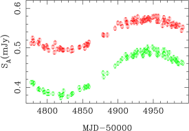
Figure 3: Two-colour light curves of Q0957+561A. These curves correspond to slightly extended versions of the LRT main fluctuations of the A image: $g$ band (circles) and $r$ band (squares).

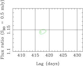
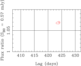
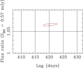
Figure 4: Best solutions and 2$\sigma$ contour lines from the $\chi^{2}$ technique. Top left panel: $\alpha$ = 3 d ($g$ band). Top right panel: $\alpha$ = 3 d ($r$ band). Bottom left panel: $\alpha$ = 9 d ($g$ band). Bottom right panel: $\alpha$ = 9 d ($r$ band).

The AB cross-correlation function is very sensitive to standard microlensing variability, i.e., uncorrelated variations in the two quasar images. If the LRT main fluctuations (left panels of Fig. 2) would be affected by microlensing, then their autocorrelation and cross-correlation functions would have different shapes, and the cross-correlation peaks would not reach a maximum value of 1 (Goicoechea et al. 1998). However, these microlensing imprints are not seen in the right panels of Fig. 2. Although slow microlensing was detected in light curves of several lensed quasars (e.g., Gaynullina et al. 2005; Fohlmeister et al. 2007; Shalyapin et al. 2009; Eulaers & Magain 2011), typical gradients are too small to play a role in brightness records over relatively short time segments. For example, Hainline et al. (2012) used LQLM I data and more recent measurements from the United States Naval Observatory (USNO) to study the $r$-band flux ratio of Q0957+561. In this analysis conducted in parallel to ours, the authors report on the possible existence of a microlensing gradient of 0.016 mag yr^-1 in the $r$ band (see, however, Section 4). Such a low gradient would produce an extrinsic variation of only 8 mmag over a six-month period, which is very much lower that the intrinsic signal that we find, and even lower than the noise level in our $r$-band data. Hence, the discussion throughout this paragraph indicates that standard microlensing is basically absent from the selected light curves and accordingly does not perturb the time delay estimates.

Despite the robustness of non-parametric methods based on correlation functions, we also considered a $\chi^{2}$ (parametric) technique to determine the time delays between the two images (e.g., Kundić et al. 1997; Ullán et al. 2006). This $\chi^{2}$ minimisation allows us to check the quality of the parametric model for relating the shapes of $S_{A}$ and $S_{B}$. The simplest model consists of a constant flux ratio, i.e., $S_{B}(t)=(B/A)S_{A}(t-\Delta t_{BA})$, where $B/A$ is a constant. However, there is evidence for a $B/A-S_{B}$ correlation (see details and a discussion of this flux ratio behaviour in Sect. 4–6), therefore we assumed an observationally motivated model: $S_{B}(t)=(B/A)S_{A}(t-\Delta t_{BA})$, $B/A=(B/A)_{0}[S_{B}(t)/S_{B0}]^{\beta}$, where $(B/A)_{0}$ is the flux ratio at the reference flux $S_{B0}$ and $\beta$ is the power-law index. Apart from the time delay $\Delta t_{BA}$, this scheme involves two additional free parameters $(B/A)_{0}$ and $\beta$, which are used to link shapes. We do not know what the true way is to link $S_{B}$ to the correlated time evolution of $S_{A}$. A power-law flux ratio is only one option among a variety of possible models, and therefore, our $\chi^{2}$ results should be taken with caution. To compare $S_{A}$ and $S_{B}$, we also used bins in A with semisize $\alpha$.

In the top panels of Fig. 4, we display $\Delta t_{BA}$-$(B/A)_{0}$ maps including our best solutions for $\alpha$ = 3 d (crosses) and their associated 2$\sigma$ contour lines. The $g$-band and $r$-band results are shown in the left and right panels, respectively. We obtained reduced chi-square values close to 1 ($\chi^{2}$/dof $\sim$ 0.9), and two disjoint delay intervals around 417 d ($g$ band) and 424 d ($r$ band). These $g$-band and $r$-band delay intervals are separated by 4 d, whereas the difference between the best solutions is 7 d. Thus we find that the chromaticity in $\Delta t_{BA}$ is more pronounced than that from the $\delta^{2}$ method (see above). Although the results for $\alpha$ = 3 d support a significant chromaticity of the delay, other values of $\alpha$ produce overlapping delay intervals. For example, if we take $\alpha$ = 9 d, the best solutions are characterised by $\chi^{2}$/dof $\sim$ 1.2–1.5. These appear in the bottom panels of Fig. 4 (crosses). We also show the 2$\sigma$ contour lines around 418 d ($g$ band; bottom left panel) and 420 d ($r$ band; bottom right panel). For $\alpha$ = 9 d, both delay intervals overlap with each other, and the parametric technique does not separate the two delays in the two optical bands. However, the production of ”excessive chromaticity” or achromaticity is not surprising, since the degeneracy between the two shape parameters and the delay likely prevents accurate/reliable $\chi^{2}$-based delay measurements.

Hereafter, we consider the self-consistent solution for the delays: (a) $\Delta t_{BA}$ = 417 d in the $g$ band, (b) $\Delta t_{BA}$ = 420 d in the $r$ band, (c) $\Delta t_{rg}$ = 4 d for the B image, and (d) $\Delta t_{rg}$ = 1 d for the A image. Our solution agrees with the discussion in the previous paragraphs of this section. We also note that several studies of $\Delta t_{BA}$ in the red part of the optical spectrum favoured delays above 417 d that are only marginally consistent with the APO 2$\sigma$ interval in the $g$ band (e.g., Serra-Ricart et al. 1999; Ovaldsen et al. 2003a). This discrepancy was not originally associated with a chromatic delay between images, but with less quasar variability and greater contamination from the lensing galaxy in red filters, the existence of multiple achromatic delays in long-term light curves, etc.

4 Two-colour flux ratio over the 2000–2010 decade

The spectral behaviour and the long-term evolution of the delay-corrected flux ratio $B/A$ has attracted increasing attention in the first decade of this century (e.g., Refsdal et al. 2000; Oscoz et al. 2002; Ovaldsen et al. 2003b; Goicoechea et al. 2005a, b). The 1999–2000 Hubble Space Telescope (HST) spectra of Q0957+561 indicated the chromaticity of $B/A$ at optical continuum wavelengths (Goicoechea et al. 2005a). At the average wavelengths of the $g$ and $r$ bands, the HST data in Fig. 1 of Goicoechea et al. (2005a) lead to 1$\sigma$ intervals $B/A$ = 1.10 $\pm$ 0.01 ($g$-band) and $B/A$ = 1.04 $\pm$ 0.02 ($r$ band). It can be also demonstrated that the C iii] ($\lambda$1909) and Mg ii ($\lambda$2798) emission lines only slightly influence the estimation of the optical continuum flux ratio from the $g$ and $r$ broad filters, introducing a small bias of $(B/A)_{\rm cont}/(B/A)_{\rm cont+line}\sim$ 1.01. Apart from spectral analyses, time domain studies suggested the constancy of the flux ratio between 1987 and 2000 ($R$ band; e.g., Oscoz et al. 2002), and then from 2000 to 2007 ($g$ and $r$ bands; Paper I). Here, the new LRT data allow us to discuss the $gr$ flux ratio in the 2007–2010 period, as well as to compare it with the HST two-colour ratio in 2000.

To evaluate the flux ratio in the $g$ band, one should compare the light curve of the B image and the fluxes of the A image shifted by + 417 d. For example, the Q0957+561B fluxes between day 3649 and day 3894 have a very short counterpart in the original light curve of Q0957+561A before day 3477 (see the circles in both panels of Fig. 1). The counterpart only consists of three data points, and we did not calculate the $g$-band flux ratio over days 3649–3894. We also emphasize the absence of a counterpart in the $r$-band fluxes of A for this time segment of B. The first useful time segment of B covers days 4010–4249, and it is labelled TS1. The fluxes of B in TS1 have a relatively long overlap with fluxes of A shifted by + 417 d (see the middle and bottom left panels of Fig. 7 in Paper I). We removed two data points from the overlapping record of A because these fluxes are affected by atmospheric and/or instrumental problems (see Paper I for details). The other useful time segments of B are: TS2 (from day 4498 to day 4627), TS3 (from day 4777 to day 4992) and TS4 (from day 5107 to day 5373).

Table 3: Flux ratio in the $g$ band.

Time segment	$\alpha$ (d)	Best fit	$\chi^{2}$/dof	$B/A$
TS1	6	1.083	46.4/50	1.078–1.089
	9	1.083	53.0/54	1.078–1.088
TS2	6	1.141	40.7/37	1.135–1.146
	9	1.143	61.3/40	–
TS3	6	1.089	41.0/44	1.085–1.094
	9	1.088	52.2/50	1.083–1.092
TS4	6	1.137	126.3/52	–
	9	1.137	152.3/54	–

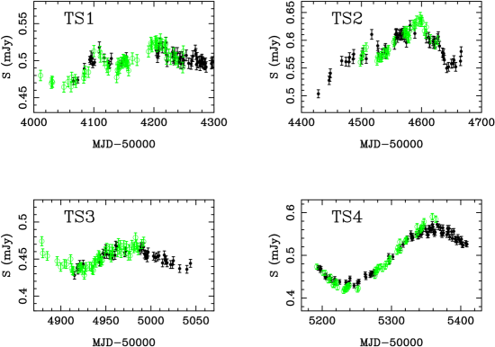
Figure 5: AB comparisons in the $g$ band. We show the overlapping periods between the light curves of A (filled circles) and B (open circles), where the fluxes of A are shifted by + 417 d and are properly amplified (see main text). Top left panel: the overlap period for the first time segment of B, i.e., TS1 (days 4010–4249). The A signal is amplified by 1.086. Top right panel: the overlap period for TS2 (days 4498–4627). The A signal is amplified by 1.14. Bottom left panel: the overlap period for TS3 (days 4777–4992). The A signal is amplified by 1.086. Bottom right panel: the overlap period for TS4 (days 5107–5373). The A signal is amplified by 1.14.

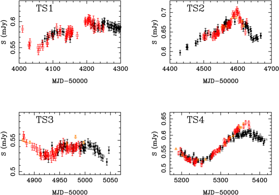
Figure 6: AB comparisons in the $r$ band. We used the original epochs and fluxes of B (open squares), while the fluxes of A are shifted by + 420 d and properly amplified (filled squares). Together with these LRT data, we also show the more poorly sampled USNO fluxes of A (filled triangles) and B (open triangles). Top and bottom left panels: comparisons in two periods of normal activity. The A signal is amplified by 1.019 (see main text). Top and bottom right panels: comparisons in two episodes of violent activity. The A signal is amplified by 1.057 (see main text).

Table 4: Flux ratio in the $r$ band.

Time segment	$\alpha$ (d)	Best fit	$\chi^{2}$/dof	$B/A$
TS1	6	1.023	50.5/46	1.019–1.027
	9	1.023	59.7/50	1.019–1.026
TS2	6	1.054	52.0/46	1.050–1.058
	9	1.056	80.5/51	–
TS3	6	1.016	39.3/48	1.012–1.019
	9	1.016	34.1/50	1.012–1.019
TS4	6	1.060	160.5/54	–
	9	1.060	169.0/57	–

We used a $\chi^{2}$ minimization to find the flux ratio for each segment. In general, the shifted epochs of A do not coincide with the epochs of B, therefore we introduce bins in A around the epochs of B (e.g., Ullán et al. 2006). These bins have a semisize $\alpha$ of 6 or 9 d. In Table 3 we give the best solutions and their reduced chi-square values, as well as some 2$\sigma$ intervals for $B/A$. A constant flux ratio $B/A$ = 1.086 works on both TS1 and TS3, and it agrees well with the corresponding HST ratio in 2000 (1.086 $\times$ 1.01 $\sim$ 1.10; see above). The AB comparisons for the time segments TS1 and TS3 are shown in the top and bottom left panels of Fig. 5, where we amplified the A signal by a factor of 1.086 (filled circles). Curiously enough, the simplest scenario (constant $B/A$) does work on TS2 and TS4, since most of the best solutions are associated with reduced chi-square values ranging from 1.5 to 2.8. These best solutions $B/A\sim$ 1.14 also differ from the ratio for TS1, TS3 and the HST observing dates. Taking an amplification of 1.14 for the signal A in TS2 and TS4, both A and B signals are compared to each other in the top and bottom right panels of Fig. 5 (A = filled circles and B = open circles). The flux ratio seems to reach ”anomalous” values during episodes of violent activity (involving flux gradients $\geq$ 0.1 mJy/100 d; TS2 and TS4), while it remains lower and basically constant in other periods with flux gradients $\leq$ 0.05 mJy/100 d. In the bottom right panel of Fig. 5, we also find evidence of a correlation between flux ratio and level of flux in TS4, i.e., $B/A<$ 1.14 at $S_{B}$ = 0.42 mJy, $B/A\sim$ 1.14 at $S_{B}\sim$ 0.5 mJy and $B/A>$ 1.14 at $S_{B}$ = 0.59 mJy. This kind of correlation is not so evident in TS2.

In Table 4 we present our results in the $r$ band. For the two periods of normal activity in TS1 and TS3, a constant flux ratio $B/A$ = 1.019 can account for the flux gap between the light curve of B and the record of A shifted by + 420 d (see Table 4 and the left panels of Fig. 6). Although the adopted solution $B/A$ = 1.019 is only marginally consistent with the analyses in both periods, this should not cause suspicion of a possible decrease of $B/A$. The best-fit $\chi^{2}$/dof values for TS3 are 0.7–0.8, so the formal 2$\sigma$ intervals for this time segment only contain reduced chi-square values equal to or less than 0.9. Consequently, there are solutions $B/A\sim$ 1.021–1.022 with $\chi^{2}$/dof $\sim$ 1, which suggest that the flux ratio uncertainty for TS3 in Table 4 is underestimated. Taking the small perturbation by the Mg ii ($\lambda$2798) line into account, we obtain a continuum flux ratio of $B/A\sim 1.019\times 1.01\sim 1.03$ at the average wavelength of the $r$ band (see above). This ratio agrees with the HST determination of $B/A$ at the same wavelength. For the two periods of violent activity (TS2 and TS4), a constant flux ratio does not convincingly explain the LRT observations. Moreover, the best solutions $B/A\sim$ 1.057 do not agree with those for TS1 and TS3. We display the AB comparisons for TS2 and TS4 in the right panels of Fig. 6, where the open squares trace the light curve of B, and the delay-corrected and amplified fluxes of A are represented by filled squares. Once again, we find evidence of a $B/A-S_{B}$ correlation in the bottom right panel of Fig. 6, but this time in the $r$ band.

As we commented in Section 3, Hainline et al. (2012) found a slow gradient in the $r$-band flux ratio (in magnitudes) of Q0957+561. They used published LRT magnitudes together with new USNO data covering a general period similar to ours. However, we do not detect any long timescale drift in our analysis with only LRT data, and this discrepancy needs more attention. First, Hainline et al. (2012) adopted a LRT-USNO photometric offset of 14.455 mag, which seems to be biased in + 0.025 mag when comparing LRT and USNO magnitudes at similar epochs. In their Fig. 2, the authors derive the flux ratio in the second time-segment (days 4100–4200; it corresponds to our TS2) from a few differences $\Delta m_{A}$(LRT) - $\Delta m_{B}$(USNO). Because the USNO fluxes are likely underestimated in 0.025 mag, these differences should be enlarged until reaching the values for the fourth time-segment (days 4750–5000; TS4 in our framework). Second, the flux ratio in the third time-segment (days 4500–4600; TS3 in our framework) is inferred from only a few USNO magnitude differences that include some outlier. In Fig. 6 we compare the LRT and USNO fluxes using an unbiased LRT-USNO photometric offset of 14.43 mag, as well as turning HJD into MJD and magnitudes into mJy. The open triangles describe the USNO light curve of B, and the delay-corrected and amplified USNO fluxes of A are displayed as filled triangles. The time delay and the amplifications are those obtained from the LRT data (see above). In general, the LRT and USNO data agree very well. However, there is a clear outlier in the USNO record of B for TS3. This noticeable deviation from the general trend means that $S_{B}$ is overestimated, and therefore, its associated magnitude should be increased by a certain amount. In Hainline et al.’s scheme, this would lead to a lower $\Delta m_{A}$ - $\Delta m_{B}$ value in the third time-segment, so the new cloud of magnitude differences would more closely resemble the cloud in the first time-segment (TS1 in our framework). Therefore, both the LRT and USNO data sets are consistent with an oscillating behaviour of $B/A$.

5 Conclusions

Our main conclusions are:

1. New LRT light curves of Q0957+561A and Q0957+561B in the $gr$ bands during 2008–2010 show well-sampled, sharp intrinsic fluctuations with $S/N\sim$ 10. These extraordinary features allowed us to very accurately determine the $g$-band and $r$-band time delays between both quasar images. The two time delays are inconsistent with each other at the 2$\sigma$ level. More specifically, while we obtain a delay near to 417 d in the $g$ band, there is an extra delay of about three days in the $r$ band. This extra delay cannot be attributed to low $S/N$ values, contamination from the main lensing galaxy, or similar artifacts.

2. From the LRT two-colour photometry of Q0957+561 during 2005–2010, we inferred the $g$-band and $r$-band delay-corrected flux ratio in four different time segments. The flux ratio $B/A$ has an oscillating behaviour in both optical bands, reaching higher values in the two segments of violent activity and remaining lower in the other two periods of normal activity. These normal activity periods are characterised by $g$-band flux gradients $\leq$ 0.05 mJy/100 d, and $B/A$ in each band does not vary from period to period or within a given period. The normal $g$-band and $r$-band ratios are also consistent with the HST ratios in 2000 at the average wavelengths of the $g$ and $r$ bands. For the two episodes of violent activity (showing $g$-band flux gradients $\geq$ 0.1 mJy/100 d), the flux ratio in each band is similar in both segments, but it seems to be correlated with the intra-segment flux level.

6 Discussion and future work

The optical continuum of Q0957+561A is plausibly affected by a dense dusty cloud inside the cD lensing galaxy at $z$ = 0.36 (Goicoechea et al. 2005a, b). Because the light propagation time in the intervening medium is expected to increase with decreasing wavelength (chromatic dispersion; e.g., Born & Wolf 1999), the presence of this substructure could be responsible for a three-day lag between $g$-band and $r$-band signals, and thus explain the observed chromaticity of the delay between images. A detailed discussion on the composition and size of the cloud along the line of sight to the A image is beyond the scope of this paper. If this scenario turns out to be true, it would be necessary to estimate the proper delay to obtain a refined delay-based determination of the Hubble constant $H_{0}$ (e.g., Jackson 2007; Fadely et al. 2010). In addition, future multi-wavelength (optical) monitoring campaigns of other gravitationally lensed quasars may also lead to unexpected delays caused by substructures in non-local lensing galaxies, and thus, to improved estimates of lensing mass distributions and $H_{0}$.

There is at least one crude interpretation for the flux ratio anomaly during violent episodes in Q0957+561. The violent activity may be related to a strong outflow, inducing a significant polarization degree in the otherwise weakly polarised UV emission (e.g., Begelman & Sikora 1987; Beloborodov 1998). For the A image, this polarised radiation would pass through a dust-rich region with alligned elongated dust grains, suffering from a higher extinction than that observed in periods of normal activity (dichroism; e.g., Born & Wolf 1999). The induced polarisation degree could increase with increasing activity of the central engine (flux level), so that more extinction would be observed for higher fluxes. Future polarimetric data in both normal and violent periods will be used to check this interpretation.

A microlensing scenario is difficult to reconcile with observations of Q0957+561 for the last 25 years. The analysis of the LRT light curves indicates the absence of uncorrelated variations in the two quasar images (standard microlensing), and only a slight $B/A$ increase occurs for the sharpest intrinsic events. To account for this flux ratio anomaly, one might invoke the possible existence of radial expansions of the accretion disc during violent episodes (a model of an accretion disc with a time-varying size has also recently been proposed by Blackburne & Kochanek 2010). The expanded sources would cover larger regions of the microlensing magnification pattern for the B image, and produce slight extra magnifications of that image. Although such an exotic microlensing seems to work, the ”excessive constancy” of $B/A$ over $\sim$ 25 years (e.g., Oscoz et al. 2002, and this paper) calls this scenario into question. We think the next logical step should be to accurately study light curves covering more than 5–6 years. New 1999–2005 IAC-80 data in the $R$ band together with the 2005–2010 LRT and 2008–2010 USNO data in the $r$ band will make up a 10-year variability database, whereas additional old $R$-band fluxes (Ovaldsen et al. 2003a; Serra-Ricart et al. 1999) and 2011–2012 frames in the $r$ band may contribute to a 20-year baseline.