Infinite Shift-invariant Grouped Multi-task Learning for Gaussian Processes

Abstract

Multi-task learning leverages shared information among data sets to improve the learning performance of individual tasks. The paper applies this framework for data where each task is a phase-shifted periodic time series. In particular, we develop a novel Bayesian nonparametric model capturing a mixture of Gaussian processes where each task is a sum of a group-specific function and a component capturing individual variation, in addition to each task being phase shifted. We develop an efficient em algorithm to learn the parameters of the model. As a special case we obtain the Gaussian mixture model and em algorithm for phased-shifted periodic time series. Furthermore, we extend the proposed model by using a Dirichlet Process prior and thereby leading to an infinite mixture model that is capable of doing automatic model selection. A Variational Bayesian approach is developed for inference in this model. Experiments in regression, classification and class discovery demonstrate the performance of the proposed models using both synthetic data and real-world time series data from astrophysics. Our methods are particularly useful when the time series are sparsely and non-synchronously sampled.

Keywords: Gaussian processes, Dirichlet process, Multi-task learning, em algorithm, Variational Inference

1 Introduction

In many real world problems we are interested in learning multiple tasks while the training set for each task is quite small. For example, in pharmacological studies, we may be attempting to predict the concentration of some drug at different times across multiple patients. Finding a good regression function of an individual patient based only on his or her measurements can be difficult due to insufficient training points for the patient. Instead, by using measurements across all the patients, we may be able to leverage common patterns across patients to obtain better estimates for the population and for each patient individually. Multi-task learning captures this intuition aiming to learn multiple correlated tasks simultaneously. This idea has attracted much interest in the literature and several approaches have been applied to a wide range of domains including medical diagnosis (Bi et al., 2008), recommendation systems (Dinuzzo et al., 2008) and HIV Therapy Screening (Bickel et al., 2008). Building on the theoretical framework for single-task learning, multi-task learning has recently been formulated by Evgeniou et al. (2006) as a multi-task regularization problem in vector-valued Reproducing Kernel Hilbert space.

Several approaches formalizing multi-task learning exist within Bayesian statistics. Considering hierarchical Bayesian models (Xue et al., 2007; Gelman, 2004), one can view the parameter sharing of the prior among tasks as a form of multi-task learning where evidence from all tasks is used to infer the parameters. Over the past few years, Bayesian models for multi-task learning were formalized using Gaussian processes (Yu et al., 2005; Schwaighofer et al., 2005; Pillonetto et al., 2010). In this mixed-effect model, information is shared among tasks by having each task combine a common (fixed effect) portion and a task specific portion, each of which is generated by an independent Gaussian process.

Our work builds on this formulation extending it and the associated algorithms in several ways. In particular, we extend the model to include three new aspects. First, we allow the fixed effect to be multi-modal so that each task may draw its fixed effect from a different cluster. Second, we extend the model so that each task may be an arbitrarily phase-shifted image of the original time series. This yields our GMT model: the shift-invariant grouped mixed-effect model. Alternatively, our model can be viewed as a probabilistic extension of the Phased K-means algorithm of Rebbapragada et al. (2009) that performs clustering for phase-shifted time series data and as a non-parametric Bayesian extension of mixtures of random effects regressions for curve clustering (Gaffney and Smyth, 2003). Finally, unlike the existing models that require the model order to be set a priori, our extension in the DP-GMT model uses a Dirichlet process prior on the mixture proportions so that the number of mixture components is adaptively determined by the data rather than being fixed explicitly.

Our main technical contribution is the inference algorithm for the proposed model. We develop details for the em algorithm for the GMT model and a Variational em for DP-GMT optimizing the maximum a posteriori (MAP) estimates for the parameters of the models. Technically, the main insights are in estimating the expectation for the coupled hidden variables (the cluster identities and the task specific portion of the time series) and in solving the regularized least squares problem for a set of phase-shifted observations. In addition, for the DP-GMT, we show that the variational em algorithm can be implemented with the same complexity as the fixed order GMT without using sampling. Thus the DP-GMT provides an efficient model selection algorithm compared to alternatives such as BIC. As a special case our algorithm yields the (Infinite) Gaussian mixture model for phase shifted time series, which may be of independent interest, and which is a generalization of the algorithms of Rebbapragada et al. (2009) and Gaffney and Smyth (2003).

Our model primarily captures regression of time series but because it is a generative model it can be used for class discovery, clustering, and classification. We demonstrate the utility of the model using several experiments with both synthetic data and real-world time series data from astrophysics. The experiments show that our model can yield superior results when compared to the single-task learning and Gaussian mixture models, especially when each individual task is sparsely and non-synchronously sampled. The DP-GMT model yields results that are competitive with model selection using BIC over the GMT model, at much reduced computational cost.

The remainder of the paper is organized as follows. Section 2 provides an introduction to the multi-task learning problem and its Bayesian interpretation and develops the main assumptions of our model. Section 3 defines the new generative model, Section 4 develops the em algorithm for it, and the infinite mixture extension is addressed in Section 5. The experimental results are reported in Section 6. Related work is discussed in Section 7 and the final section concludes with a discussion and outlines ideas for future work.

2 Preliminaries

Throughout the paper, scalars are denoted using italics, as in $x,y\in{\rm I\!R}$; vectors use bold typeface, as in $\mathbf{x},\mathbf{y}$, and $x_{i}$ denotes the $i$th entry of $\mathbf{x}$. For a vector $\mathbf{x}$ and real valued function $f:{\rm I\!R}\rightarrow{\rm I\!R}$, we extend the notation for $f$ to vectors so that $f(\mathbf{x})=[f(x_{1}),\cdots,f(x_{n})]^{\mathrm{T}}$ where the superscript $\mathrm{T}$ stands for transposition (and the result is a column vector). $\mathcal{K}(\cdot,\cdot)$ denotes a kernel function associated to some reproducing kernel Hilbert space (RKHS) $\mathcal{H}$ and its norm is denoted as $\|\cdot\|_{\mathcal{H}}$. To keep the notation simple, $\sum_{j=1}^{M}$ is substituted by $\sum_{j}$ where the index $j$ is not confusing.

2.1 Multi-task learning with kernel

Given training set $\mathcal{D}=\{\mathbf{x}_{i},y_{i}\},i=1,\cdots,N$, where $\mathbf{x}_{i}=[x_{i1},x_{i2},\cdots,x_{id}]^{\mathrm{T}}\in\mathcal{X}\subset{\rm I\!R}^{d}$, single-task learning focuses on finding a function $f:\mathcal{X}\rightarrow{\rm I\!R}$ that best fits and generalizes the observed data. In the regularization framework, learning $f$ amounts to solving the following variational problem (Evgeniou et al., 2000; Scholkopf and Smola, 2002)

$$f^{*}=\underset{f\in\mathcal{H}}{\text{argmin}}\left\{\sum_{i}V(f(\mathbf{x}_{i}),y_{i})+\lambda\|f\|^{2}_{\mathcal{H}}\right\}$$ (1)

where $V(\cdot,\cdot)$ is some (typically convex) loss function. The norm $\|\cdot\|_{\mathcal{H}}$ relates to regularity condition on the function where a large norm penalizes non-smooth functions. The regularization parameter $\lambda$ provides a tradeoff between the loss term and the complexity of the function.

Consider a set of $M$ tasks, with $j$th task $\mathcal{D}^{j}=(\mathbf{x}_{i}^{j},y_{i}^{j}),i=1,2,\cdots,n_{j}$. Multi-task learning seeks to find $f^{j}$ for each task simultaneously, which, assuming square loss function, can be formulated as the following regularization problem

$$\underset{f^{1},\cdots,f^{M}\in\mathcal{H}}{\text{argmin}}\left\{\frac{1}{M}\sum_{j=1}^{M}\sum_{i=1}^{n_{j}}(y^{j}_{i}-f^{j}(\mathbf{x}^{j}_{i}))^{2}+\lambda\text{PEN}(f^{1},f^{2},\cdots,f^{j})\right\}$$ (2)

where the penalty term, applying jointly to all the tasks, encodes our prior information on how smooth the functions are, as well as how these tasks are correlated with each other. For example, setting the penalty term to $\sum_{j}\|f^{j}\|_{\mathcal{H}}$ implies that there is no correlation among the tasks. It further decomposes the optimization functional to $M$ separate single-task learning problems. On the other hand, with a shared penalty, the joint regularization can lead to improved performance. Moreover, we can use a norm in RKHS with a multi-task kernel to incorporate the penalty term (Micchelli and Pontil, 2005). Formally, consider a vector-valued function $f:\mathcal{X}\rightarrow{\rm I\!R}^{M}$ defined as $f\triangleq[f^{1},f^{2},\cdots,f^{M}]^{\mathrm{T}}$. Then Equation (2) can be written as

$$\underset{f\in\mathcal{H}}{\text{argmin}}\left\{\frac{1}{M}\sum_{j=1}^{M}\sum_{i=1}^{n_{j}}(y^{j}_{i}-f^{j}(\mathbf{x}^{j}_{i}))^{2}+\lambda\|f\|_{\mathcal{H}}^{2}\right\}$$ (3)

where $\|\cdot\|_{\mathcal{H}}$ is the norm in RKHS with the multi-task kernel $\mathcal{Q}:(\mathbf{\Lambda},\mathcal{X})\times(\mathbf{\Lambda},\mathcal{X})\rightarrow{\rm I\!R}$, where $\mathbf{\Lambda}=\{1,2,\cdots,M\}$. As shown by Evgeniou et al. (2006), the representer theorem gives the form of the solution to Equation (3)

$$f^{\ell}(\cdot)=\sum_{j=1}^{M}\sum_{i=1}^{n_{j}}c_{i}^{j}\mathcal{Q}((\cdot,\ell),(\mathbf{x}_{i}^{j},j))$$ (4)

with norm

$$\|f\|_{\mathcal{Q}}^{2}=\sum_{\ell,k}\sum_{i=1}^{n_{\ell}}\sum_{j=1}^{n_{k}}c_{i}^{\ell}c_{j}^{k}\mathcal{Q}((\mathbf{x}_{i}^{\ell},\ell),(\mathbf{x}_{j}^{k},k)).$$

Let $\mathbf{C}=[{c}_{1}^{1},{c}_{2}^{1},\cdots,{c}_{n_{M}}^{M}]^{\mathrm{T}},\mathbf{Y}=[y^{1}_{1},y^{1}_{2},\cdots,y^{M}_{n_{M}}]^{\mathrm{T}}\in{\rm I\!R}^{\sum_{j}n_{j}}$ and $\mathbf{X}=[\mathbf{x}^{1}_{1},\mathbf{x}^{1}_{2},\cdots,\mathbf{x}^{M}_{n_{M}}]$, then the coefficients $\{c_{i}^{j}\}$ are given by the following linear system

$$(\mathbf{Q}+\lambda\mathbb{I})\mathbf{C}=\mathbf{Y}$$ (5)

where $\mathbf{Q}\in{\rm I\!R}^{\sum_{j}n_{j}\times\sum_{j}n_{j}}$ is the kernel matrix formed by $\mathbf{X}$.

2.2 Bayesian formulation

A Gaussian process is a functional extension for Multivariate Gaussian distributions. In the Bayesian literature, it has been widely used in statistical models by substituting a parametric latent function with a stochastic process with a Gaussian prior  (Rasmussen, 2006). More precisely, under the single-task setting a simple Gaussian regression model is given by

$$y=f(\mathbf{x})+\epsilon$$

where $f$’s prior is a zero mean Gaussian process with covariance function $\mathcal{K}$ and $\epsilon$ is independent zero mean white noise with variance $\sigma^{2}$. Given data set $\mathcal{D}=\{\mathbf{x}_{i},y_{i}\},i=1,\cdots,N$, let $\mathbf{K}=(\mathcal{K}(\mathbf{x}_{i},\mathbf{x}_{j}))_{i,j}$, then $\mathbf{f}\triangleq[f(\mathbf{x}_{1}),\cdots,f(\mathbf{x}_{N})]^{\mathrm{T}}\sim\mathcal{N}(\mathbf{0},\mathbf{K})$ and the posterior on $\mathbf{f}$ is given by

$$\Pr(\mathbf{f}|\mathcal{D})=\mathcal{N}(\mathbf{K}(\sigma^{2}\mathbb{I}+\mathbf{K})^{-1}\mathbf{y},\sigma^{2}(\sigma^{2}\mathbb{I}+\mathbf{K})^{-1}\mathbf{K}).$$

The predictive distribution for some test point $\mathbf{x}_{*}$ distinct from the training examples is

$$\begin{split}\Pr(f(\mathbf{x}_{*})|\mathbf{x}_{*},\mathcal{D})&=\int\Pr(f(\mathbf{x}_{*})|\mathbf{x}_{*},f)\Pr(f|\mathcal{D})df\\ &=\mathcal{N}\left(\mathbf{k}(\mathbf{x}_{*})^{\mathrm{T}}(\sigma^{2}\mathbb{I}+\mathbf{K})^{-1}\mathbf{y},\mathcal{K}(\mathbf{x}_{*},\mathbf{x}_{*})-\mathbf{k}(\mathbf{x}_{*})^{\mathrm{T}}(\sigma^{2}\mathbb{I}+\mathbf{K})^{-1}\mathbf{k}(\mathbf{x}_{*})\right)\end{split}$$

where $\mathbf{k}(\mathbf{x}_{*})=[\mathcal{K}(\mathbf{x}_{1},\mathbf{x}_{*}),\cdots,\mathcal{K}(\mathbf{x}_{N},\mathbf{x}_{*})]^{\mathrm{T}}$. Furthermore, under square loss function, the optimizer of Equation (1) is equal to the expectation of the predictive distribution (Rasmussen, 2006). Finally, a Gaussian process $f$ corresponds to a RKHS $\mathcal{H}$ with kernel $\mathcal{K}$ such that

$$\text{cov}[f(\mathbf{x}),f(\mathbf{y})]=\mathcal{K}(\mathbf{x},\mathbf{y})\quad\forall\mathbf{x},\mathbf{y}\in\mathcal{X}.$$ (6)

In this way, we can express a prior on functions $f$ using a zero mean Gaussian process (Lu et al., 2008)

$$\begin{split}f&\sim\exp\left\{-\frac{1}{2}\|f\|_{\mathcal{H}}^{2}\right\}.\\ \end{split}$$ (7)

Applying this framework in the context of multi-task learning, the model is given by

$$\mathbf{y}^{j}_{i}=f^{j}(\mathbf{x}^{j}_{i})+\epsilon_{ij}$$

where $f^{j}$ are zero mean Gaussian processes and $\epsilon_{ij}$ captures i.i.d. zero-mean noise with variance $\sigma^{2}$. Pillonetto et al. (2010) formalize the connection between multi-task kernel $\mathcal{Q}$ and covariance function among $\{f^{j}\}$ using

$$\text{cov}[f^{i}(\mathbf{x}),f^{j}(\mathbf{x}^{\prime})]=\mathcal{Q}((\mathbf{x},i),(\mathbf{x}^{\prime},j)),\quad i,j=1,\cdots,M.$$ (8)

2.3 Basic Model Assumptions

Given data $\{\mathcal{D}^{j}\}$, the so-called nonparametric Bayesian mixed-effect model (Lu et al., 2008; Pillonetto et al., 2010) captures each task $f^{j}$ with respect to $\mathcal{D}^{j}$ using a sum of an average effect function and an individual variation for each specific task,

$$f^{j}(x)=\bar{f}(x)+\tilde{f}^{j}(x),\quad j=1,\cdots,M.$$

This assumes that the fixed-effect (mean function) $\bar{f}$ is sufficient to capture the behavior of the data, an assumption that is problematic for distributions with several modes. To address this, we introduce a mixture model allowing for multiple modes (just like standard Gaussian mixture model (GMM)), but maintaining the formulation using Gaussian processes. This amounts to adding a group effect structure and leads to the following assumption:

Assumption 1

For each $j$ and $\mathbf{x}\in\mathcal{X}$,

$$f^{j}(\mathbf{x})=\bar{f}_{z_{j}}(\mathbf{x})+\tilde{f}^{j}(\mathbf{x}),\quad j=1,\cdots,M$$ (9)

where $\{\bar{f}_{s}\},s=1,\cdots,k$ and $\tilde{f}^{j}$ are zero-mean Gaussian processes and $z_{j}\in\{1,\cdots,k\}$. In addition, $\{\bar{f}_{s}\}$ and $\tilde{f}^{j}$ are assumed to be mutually independent.

With the grouped-effect model and groups predefined, one can define a kernel that relates (with non zero similarity) only points from the same example or points for different examples but the same center as follows

$$\mathcal{Q}((\mathbf{x},i),(\mathbf{x}^{\prime},j))=\delta_{z_{i},z_{j}}\overline{\mathcal{K}}_{z_{i}}(\mathbf{x},\mathbf{x}^{\prime})+\delta_{i,j}\widetilde{\mathcal{K}}_{i}(\mathbf{x},\mathbf{x}^{\prime})$$

where

$$\begin{cases}\overline{\mathcal{K}}_{z_{i}}(\mathbf{x},\mathbf{x}^{\prime})=\text{cov}[\bar{f}_{z_{i}}(\mathbf{x}),\bar{f}_{z_{i}}(\mathbf{x}^{\prime})],\\ \widetilde{\mathcal{K}}_{i}(\mathbf{x},\mathbf{x}^{\prime})=\text{cov}[\tilde{f}^{j}(\mathbf{x}),\tilde{f}^{j}(\mathbf{x}^{\prime})].\end{cases}$$

However, in our work the groups are not known in advance and we cannot use this formulation. Instead we use a single kernel to relate all tasks.

The second extension allows us to handle phase shifted time series. In some applications, we face the challenge of learning a periodic function $f^{j}:{\rm I\!R}\rightarrow{\rm I\!R}$ on a single period $T$ from samples $\mathcal{D}=\{\mathbf{x}^{j},\mathbf{y}^{j}\},\mathbf{x}^{j},\mathbf{y}^{j}\in{\rm I\!R}^{n_{j}},j=1,\cdots,M$, where similar functions in a group differ only in their phase. In the following assumption, the model of primary focus in this paper is presented, which extends the mixed-effect model to capture both shift-invariance and the clustering property.

Assumption 2

For each $j$ and $x\in[0,T)$,

$$f^{j}(x)=[\bar{f}_{z_{j}}*\delta_{t_{j}}](x)+\tilde{f}^{j}(x),\quad,j=1,\cdots,M$$ (10)

where $z_{j}\in\{1,\cdots,k\}$, $\{\bar{f}_{s}\},s=1,\cdots,k$ and $\tilde{f}^{j}$ are zero-mean Gaussian processes, $*$ stands for circular convolution and $\delta_{t_{j}}$ is the Dirac $\delta$ function with support at $t_{j}\in[0,T)$. In addition, $\{\bar{f}_{s}\},\tilde{f}^{j}$ are assumed to be mutually independent.

3 Shift-invariant Grouped mixed-effect model

In Assumption 1, if we know the cluster assignment of each task, then the model decomposes to $k$ mixed-effect models which is the case investigated in (Pillonetto et al., 2010; Evgeniou et al., 2006). Similar results can be obtained for Assumption 2. However, prior knowledge of cluster membership is often not realistic. In this section, based on Assumption 2, a probabilistic generative model is formulated to capture the case of unknown clusters. We start by formally defining the generative model, which we call Shift-invariant Grouped mixed-effect Model (GMT). In this model, $k$ group effect functions are assumed to share the same Gaussian prior characterized by $\mathcal{K}_{0}$. The individual effect functions are Gaussian processes with covariance function $\mathcal{K}$. The model is shown in Figure 1 and it is characterized by parameter set $\mathcal{M}=\{\mathcal{K}_{0},\mathcal{K},\boldsymbol{\alpha},\{t_{j}\},\sigma^{2}\}$ and summarized as follows

1. Draw $\bar{f}_{s}|\mathcal{K}_{0}\sim\exp\left\{-\frac{1}{2}\|\bar{f}_{s}\|_{\mathcal{H}_{0}}^{2}\right\},\quad s=1,2,\cdots,k$

2. For the $j$th time series

   • Draw $z_{j}|\mathbf{\boldsymbol{\alpha}}\sim\text{Discrete}(\mathbf{\boldsymbol{\alpha}})$

   • Draw $\tilde{f}^{j}|\mathcal{K}\sim\exp\left\{-\frac{1}{2}\|\tilde{f}^{j}\|_{\mathcal{H}}^{2}\right\}$

   • Draw $\mathbf{y}^{j}|z_{j},f^{j},\mathbf{x}^{j},t_{j},\sigma^{2}\sim\mathcal{N}\left(f^{j}(\mathbf{x}^{j}),\sigma^{2}\mathbb{I}\right)$, where $f^{j}=\bar{f}_{z_{j}}*\delta_{t_{j}}+\tilde{f}^{j}$

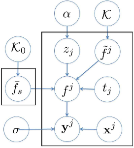
Figure 1: GMT: Plate graph

where $\boldsymbol{\alpha}$ is the mixture proportion. Additionally, denote $\mathcal{X}=\{\mathbf{x}^{1},\mathbf{x}^{2},\cdots,\mathbf{x}^{M}\}$ and $\mathcal{Y}=\{\mathbf{y}^{1},\mathbf{y}^{2},\cdots,\mathbf{y}^{M}\}$, where $\mathbf{x}^{j}$ are the time points when each time series is sampled and $\mathbf{y}^{j}$ are the corresponding observations.

We assume that the group effect kernel $\mathcal{K}_{0}$ and the number of centers $k$ are known. The assumption on $\mathcal{K}_{0}$ is reasonable, in that normally we can get more information on the shape of the mean waveforms, thereby making it possible to design kernel for $\mathcal{H}_{0}$. On the other hand, the individual variations are more arbitrary and therefore $\mathcal{K}$ is not assumed to be known. The assumption that $k$ is known requires some form of model selection. An extension using a non-parametric Bayesian model, the Dirichlet process (Teh, 2010), that does not limit $k$ is discussed in the section 5. The group effect $\{\bar{f}_{s}\}$, individual shifts $\{t_{j}\}$, noise variance $\sigma^{2}$ and the kernel for individual variations $\mathcal{K}$ are unknown and need to be estimated. The cluster assignments $\{z_{j}\}$ and individual variation $\{\tilde{f}^{j}\}$ are treated as hidden variables. Note that one could treat $\{\bar{f}_{s}\}$ too as hidden variables, but we prefer to get a concrete estimate for these variables because of their role as the mean waveforms in our model.

The model above is a standard model for regression. We propose to use it for classification by learning a mixture model for each class and using the Maximum A Posteriori (MAP) probability for the class for classification. In particular, consider a training set that has $L$ classes, where the $j$th instance is given by $\mathcal{D}^{j}=(\mathbf{x}^{j},\mathbf{y}^{j},o^{j})\in{\rm I\!R}^{n_{j}}\times{\rm I\!R}^{n_{j}}\times\{1,2,\cdots,L\}$. Each observation $(\mathbf{x}^{j},\mathbf{y}^{j})$ is given a label from $\{1,2,\cdots,L\}$. The problem is to learn the model $\mathrm{M}_{\ell}$ for each class ($L$ in total) separately and the classification rule for a new instance $(\mathbf{x},\mathbf{y})$ is given by

$$o=\underset{\ell=\{1,\cdots,L\}}{\text{argmax}}\Pr(\mathbf{y}|\mathbf{x};\mathrm{M}_{\ell})\Pr(\ell).$$ (11)

As we show in our experiments, the generative model can provide explanatory power for the application while giving excellent classification performance.

4 Parameter Estimation

Given data set $\mathcal{D}=\{\mathbf{x}^{j},\mathbf{y}^{j}\}=\{x_{i}^{j},y_{i}^{j}\},i=1,\cdots,n_{j},j=1,\cdots,M$, the learning process aims to find the MAP estimates of the parameter set $\mathcal{M}=\{\boldsymbol{\alpha},\{\bar{f}_{s}\},\{t_{j}\},\sigma^{2},\mathcal{K}\}$

$$\mathcal{M}^{*}=\underset{\mathcal{M}}{\text{argmax}}\left(\Pr(\mathcal{Y}|\mathcal{X};\mathcal{M})\times\Pr[\{\bar{f}_{s}\};\mathcal{K}_{0}]\right).$$ (12)

The direct optimization of Equation (12) is analytically intractable because of coupled sums that come from the mixture distribution. To solve this problem, we resort to the em algorithm (Dempster et al., 1977). The em algorithm is an iterative method for optimizing the maximum likelihood (ML) or MAP estimates of the parameters in the context of hidden variables. In our case, the hidden variables are $\mathbf{z}=\{z_{j}\}$ (which is the same as in standard GMM), and $\mathbf{f}=\{\mathbf{f}_{j}\triangleq\tilde{f}^{j}(\mathbf{x}^{j})\},j=1,\cdots,M$. The algorithm iterates between the following expectation and maximization steps until it converges to a local maximum.

4.1 Expectation step

In the E-step, we calculate

$$Q(\mathcal{M},\mathcal{M}^{g})={\rm I\!E}_{\{\mathbf{z},\mathbf{f}|\mathcal{X,Y};\mathcal{M}^{g}\}}\left[\log\left\{\Pr(\mathcal{Y},\mathbf{f,z}|\mathcal{X};\mathcal{M})\times\Pr[\{\bar{f}_{s}\};\mathcal{K}_{0}]\right\}\right]$$ (13)

where $\mathcal{M}^{g}$ stands for estimated parameters from the last iteration. For our model, the difficulty comes from estimating the expectation with respect to the coupled latent variables $\{\mathbf{z},\mathbf{f}\}$. In the following, we show how this can be done. First notice that,

$$\Pr(\mathbf{z},\mathbf{f}|\mathcal{X,Y};\mathcal{M}^{g})=\prod_{j}\Pr(z_{j},\mathbf{f}_{j}|\mathcal{X,Y};\mathcal{M}^{g})$$

and further that

$$\Pr(z_{j},\mathbf{f}_{j}|\mathcal{X,Y};\mathcal{M}^{g})=\Pr(z_{j}|\mathbf{x}^{j},\mathbf{y}^{j};\mathcal{M}^{g})\times\Pr(\mathbf{f}_{j}|z_{j},\mathbf{x}^{j},\mathbf{y}^{j};\mathcal{M}^{g}).$$ (14)

The first term in Equation (14) can be further written as

$$\begin{split}\Pr(z_{j}|\mathbf{x}^{j},\mathbf{y}^{j};\mathcal{M}^{g})&\propto\Pr(z_{j};\mathcal{M}^{g})\Pr(\mathbf{y}^{j}|z_{j},\mathbf{x}^{j};\mathcal{M}^{g})\\ &=\Pr(z_{j};\mathcal{M}^{g})\int\Pr(\mathbf{y}^{j},\mathbf{f}_{j}|z_{j},\mathbf{x}^{j};\mathcal{M}^{g})d\mathbf{f}_{j}\\ &=\Pr(z_{j};\mathcal{M}^{g})\int\Pr(\mathbf{y}^{j}|\mathbf{f}_{j},z_{j},\mathbf{x}^{j};\mathcal{M}^{g})\Pr(\mathbf{f}_{j};\mathcal{M}^{g})d\mathbf{f}_{j}\end{split}$$ (15)

where $\Pr(z_{j};\mathcal{M}^{g})$ is specified by the parameters estimated from last iteration. Since $z_{j}$ is given, the second term is the marginal distribution that can be calculated using a Gaussian process regression model. In particular, denoting $\mathbf{\bar{f}}^{j}=\bar{f}_{z_{j}}*\delta_{t_{j}}(\mathbf{x}^{j})$ we get

$$\begin{bmatrix}\mathbf{y}^{j}\\ \mathbf{f}^{j}\end{bmatrix}\sim\mathcal{N}\left(\begin{bmatrix}\mathbf{\bar{f}}^{j}\\ 0\end{bmatrix},\begin{bmatrix}\mathbf{K}^{g}_{j}+\sigma^{2}\mathbb{I}&\quad\mathbf{K}^{g}_{j}\\ \mathbf{K}^{g}_{j}&\quad\mathbf{K}^{g}_{j}\end{bmatrix}\right)$$

where $\mathbf{K}^{g}_{j}$ is the kernel matrix for the $j$th task using parameters from last iteration, i.e. $\mathbf{K}^{g}_{j}=(\mathcal{K}(x_{i}^{j},x_{l}^{j}))_{il}$. Therefore, the marginal distribution is

$$\mathbf{y}^{j}|z_{j}\sim\mathcal{N}(\mathbf{\bar{f}}^{j},\mathbf{K}^{g}_{j}+\sigma^{2}\mathbb{I}).$$ (16)

Next consider the second term in Equation (14). Given $z_{j}$, we know that $f^{j}=\bar{f}_{z_{j}}+\tilde{f}^{j}$, i.e. there is no uncertainty about the identity of $\bar{f}_{z_{j}}$ and therefore the calculation amounts to estimating the posterior distribution under standard Gaussian process regression, that is

$$\begin{split}&\mathbf{y}^{j}-\mathbf{\bar{f}}^{j}\sim\mathcal{N}(\tilde{f}^{j}(\mathbf{x}^{j}),\sigma^{2}\mathbb{I})\\ &\qquad\tilde{f}^{j}\sim\exp\left\{-\frac{1}{2}\|\tilde{f}^{j}\|_{\mathcal{K}}^{2}\right\}\\ \end{split}$$

and the conditional distribution is given by

$$\mathbf{f}_{j}|z_{j},\mathbf{x}^{j},\mathbf{y}^{j}\sim\mathcal{N}(\mu^{g}_{j},\mathbf{C}^{g}_{j})$$ (17)

where $\mathbf{\mu}^{g}_{j}$ is the posterior mean

$$\mathbf{\mu}^{g}_{j}=\mathbf{K}^{g}_{j}(\mathbf{K}^{g}_{j}+\sigma^{2}\mathbb{I})^{-1}(\mathbf{y}^{j}-\mathbf{\bar{f}}^{j})$$ (18)

and $\mathbf{C}_{j}^{g}$ is the posterior covariance of $\mathbf{f}_{j}$

$$\mathbf{C}_{j}^{g}=\mathbf{K}^{g}_{j}-\mathbf{K}^{g}_{j}(\mathbf{K}^{g}_{j}+\sigma^{2}\mathbb{I})^{-1}\mathbf{K}^{g}_{j}.$$ (19)

Since Equation (15) is multinomial and $\mathbf{f}_{j}$ is Normal in (17), the marginal distribution of $\mathbf{f}_{j}$ is a Gaussian mixture distribution given by

$$\begin{split}\Pr(\mathbf{f}_{j}|\mathbf{x}^{j},\mathbf{y}^{j};\mathcal{M}^{g})&=\sum_{s}\Pr(z_{j}=s|\mathbf{x}^{j},\mathbf{y}^{j};\mathcal{M}^{g})\\ &\qquad\qquad\times\mathcal{N}\left(\mu_{j},\mathbf{C}_{j}|z_{j}=s;\mathcal{M}^{g}\right),\quad s=1,\cdots,k.\end{split}$$

To work out the concrete form of $Q(\mathcal{M},\mathcal{M}^{g})$, denote $z_{il}=1$ iff $z_{i}=l$. Then the complete data likelihood can be reformulated as

$$\begin{split}\mathcal{L}&=\Pr(\mathcal{Y},\mathbf{f,z};\mathcal{X,M})\\ &=\prod_{j}\prod_{s}\left[\alpha_{s}\Pr(\mathbf{y}^{j},\mathbf{f}_{j}|z_{j}=s;\mathcal{M})\right]^{z_{js}}\\ &=\prod_{j}\prod_{s}\left[\alpha_{s}\Pr(\mathbf{y}^{j}|\mathbf{f}_{j},z_{j}=s;\mathcal{M})\Pr(\mathbf{f}_{j};\mathcal{M})\right]^{z_{js}}\\ \end{split}$$

where we have used the fact that exactly one $z_{js}$ is 1 for each $j$ and included the last term inside the product over $s$ for convenience. Then Equation (13) can be written as

$$\begin{split}Q(\mathcal{M},\mathcal{M}^{g})&=-\frac{1}{2}\sum_{s}\|f_{s}\|_{\mathcal{H}_{0}}^{2}+{\rm I\!E}_{\{\mathbf{z,f}|\mathcal{X,Y;M}^{g}\}}\left[\log\mathcal{L}\right].\end{split}$$

Denote the second term by $\widetilde{Q}$. By a version of Fubini’s theorem (Stein and Shakarchi, 2005) we have

$$\begin{split}\widetilde{Q}&={\rm I\!E}_{\{\mathbf{z}|\mathcal{X,Y;M}^{g}\}}{\rm I\!E}_{\{\mathbf{f}|\mathbf{z},\mathcal{X,Y;M}^{g}\}}\left[\log\mathcal{L}\right]\\ &=\sum_{\mathbf{z}}\Pr(\mathbf{z}|\mathcal{X,Y;M}^{g})\Bigg{\{}\sum_{j}\sum_{s}z_{js}\\ &\qquad\times\int d\Pr(\mathbf{f}_{j}|z_{j}=s)\log\left[\alpha_{s}\Pr(\mathbf{y}^{j}|\mathbf{f}_{j},z_{j}=s;\mathcal{M})\Pr(\mathbf{f}_{j};\mathcal{M})\right]\Bigg{\}}.\\ \end{split}$$ (20)

Now because the last term in Equation (20) does not include any $z_{i}$, the equation can be further decomposed as

$$\begin{split}\widetilde{Q}&=\sum_{j}\sum_{s}\left(\sum_{\mathbf{z}}\Pr(\mathbf{z}|\mathcal{X,Y;M}^{g})z_{js}\right)\\ &\qquad\times\left\{\int d\Pr(\mathbf{f}_{j}|z_{j}=s)\log[\alpha_{s}\Pr(\mathbf{y}^{j}|\mathbf{f}_{j},z_{j}=s;\mathcal{M})\Pr(\mathbf{f}_{j};\mathcal{M})]\right\}\\ &=\sum_{j}\sum_{s}\gamma_{js}\int d\Pr(\mathbf{f}_{j}|z_{j}=s)\log\left[\alpha_{s}\Pr(\mathbf{y}^{j}|\mathbf{f}_{j},z_{j}=s;\mathcal{M})\Pr(\mathbf{f}_{j};\mathcal{M})\right]\\ &=\sum_{j}\sum_{s}\gamma_{js}{\rm I\!E}_{\{\mathbf{f}_{j}|z_{j}=s,\mathbf{x}^{j},\mathbf{y}^{j};\mathcal{M}^{g}\}}\left[\log\alpha_{s}+\log\left(\Pr(\mathbf{y}^{j}|\mathbf{f}_{j},z_{j}=s;\mathcal{M})\right)+\log\left(\Pr(\mathbf{f}_{j};\mathcal{M})\right)\right]\end{split}$$ (21)

where

$$\gamma_{js}={\rm I\!E}[z_{js}|\mathbf{y}^{j},\mathbf{x}^{j};\mathcal{M}^{g}]=\frac{\Pr({z}_{j}=s|\mathbf{x}^{j},\mathbf{y}^{j};\mathcal{M}^{g})}{\sum_{s}\Pr({z}_{j}=s|\mathbf{x}^{j},\mathbf{y}^{j};\mathcal{M}^{g})}$$ (22)

can be calculated from Equation (15) and (16) and $\gamma_{js}$ can be viewed as a fractional label indicating how likely the $j$th task is to belong to the $s$th group. Recall that $\Pr(\mathbf{y}^{j}|\mathbf{f}_{j},z_{j}=s)$ is a normal distribution given by $\mathcal{N}([\bar{f}_{z_{j}}*\delta_{t_{j}}](\mathbf{x}^{j})+\mathbf{f}_{j},\sigma^{2}\mathbb{I})$ and $\Pr(\mathbf{f}_{j};\mathcal{M})$ is a standard multivariate Gaussian distribution determined by its prior

$$\Pr(\mathbf{f}_{j};\mathcal{M})=\frac{1}{\sqrt{(2\pi)^{n_{j}}|\mathbf{K}_{j}|}}\exp\left\{-\frac{1}{2}\mathbf{f}_{j}^{T}\mathbf{K}_{j}^{-1}\mathbf{f}_{j}\right\}.$$

Using these facts and Equation (21), $Q(\mathcal{M},\mathcal{M}^{g})$ can be re-formulated as

$$\begin{split}Q(\mathcal{M},\mathcal{M}^{g})&=-\frac{1}{2}\sum_{s}\|\bar{f}_{s}\|_{\mathcal{H}_{0}}^{2}-\sum_{j}n_{j}\log\sigma+\sum_{j}\sum_{s}\gamma_{js}\log\alpha_{s}\\ &\qquad-\frac{1}{2\sigma^{2}}\sum_{j}\sum_{s}\gamma_{js}{\rm I\!E}_{\{\mathbf{f}_{j}|z_{j}=s,\mathbf{x}^{j},\mathbf{y}^{j};\mathcal{M}^{g}\}}\left[\|\mathbf{y}^{j}-[\bar{f}_{s}*\delta_{t_{j}}](\mathbf{x}^{j})-\mathbf{f}_{j}\|^{2}\right]\\ &\qquad-\frac{1}{2}\sum_{j}\log|\mathbf{K}_{j}|-\frac{1}{2}\sum_{j}\sum_{s}\gamma_{js}{\rm I\!E}_{\{\mathbf{f}_{j}|z_{j}=s,\mathbf{x}^{j},\mathbf{y}^{j};\mathcal{M}^{g}\}}\left(\mathbf{f}^{\mathrm{T}}_{j}\mathbf{K}^{-1}_{j}\mathbf{f}_{j}\right)\end{split}$$ (23)

We next develop explicit closed forms for the remaining expectations. For the first, note that for $\mathbf{x}\sim\mathcal{N}(\mu,\mathbf{\Sigma})$ and a constant vector $\mathbf{a}$,

$$\begin{split}{\rm I\!E}[\|\mathbf{a}-\mathbf{x}\|^{2}]&={\rm I\!E}[\|\mathbf{a}\|^{2}-2\langle\mathbf{a},\mathbf{x}\rangle+\|\mathbf{x}\|^{2}]\\ &=\|\mathbf{a}\|^{2}-2\langle\mathbf{a},{\rm I\!E}[\mathbf{x}]\rangle+{\rm I\!E}[\mathbf{x}]^{2}+\text{Tr}(\mathbf{\Sigma})\\ &=\|\mathbf{a}-\mu\|^{2}+\text{Tr}(\mathbf{\Sigma}).\end{split}$$

Therefore the expectation is

$$\begin{split}{\rm I\!E}_{\{\mathbf{f}_{j}|z_{j}=s,\mathbf{x}^{j},\mathbf{y}^{j};\mathcal{M}^{g}\}}&\left[\|\mathbf{y}^{j}-[\bar{f}_{s}*\delta_{t_{j}}](\mathbf{x}^{j})-\mathbf{f}_{j}\|^{2}\right]=\frac{1}{2\sigma^{2}}\sum_{j}\text{Tr}(\mathbf{C}_{j}^{g})\\ &\qquad+\frac{1}{2\sigma^{2}}\sum_{j}\sum_{s}\gamma_{js}\left(\|\mathbf{y}^{j}-[f_{s}*\delta_{t_{j}}](\mathbf{x}^{j})-\mu_{js}\|^{2}\right)\\ \end{split}$$ (24)

where $\mu_{js}={\rm I\!E}_{\{\mathbf{f}_{j}|z_{j}=s,\mathbf{x}^{j},\mathbf{y}^{j};\mathcal{M}^{g}\}}[\mathbf{f}_{j}]$ is as in Equation (18) where we set $z_{j}=s$ explicitly.

For the second expectation we have

$$\begin{split}{\rm I\!E}_{\{\mathbf{f}_{j}|z_{j}=s,\mathbf{x}^{j},\mathbf{y}^{j};\mathcal{M}^{g}\}}\left(\mathbf{f}^{\mathrm{T}}_{j}\mathbf{K}^{-1}_{j}\mathbf{f}_{j}\right)&={\rm I\!E}_{\{\mathbf{f}_{j}|z_{j}=s,\mathbf{x}^{j},\mathbf{y}^{j};\mathcal{M}^{g}\}}\left[\text{Tr}\left(\mathbf{f}^{\mathrm{T}}_{j}\mathbf{K}^{-1}_{j}\mathbf{f}_{j}\right)\right]\\ &={\rm I\!E}_{\{\mathbf{f}_{j}|z_{j}=s,\mathbf{x}^{j},\mathbf{y}^{j};\mathcal{M}^{g}\}}\left[\text{Tr}\left(\mathbf{K}^{-1}_{j}\mathbf{f}_{j}\mathbf{f}^{\mathrm{T}}_{j}\right)\right]\\ &=\text{Tr}\left({\rm I\!E}_{\{\mathbf{f}_{j}|z_{j}=s,\mathbf{x}^{j},\mathbf{y}^{j};\mathcal{M}^{g}\}}[\mathbf{K}^{-1}_{j}\mathbf{f}_{j}\mathbf{f}^{\mathrm{T}}_{j}]\right)\\ &=\text{Tr}\left(\mathbf{K}_{j}^{-1}(\mathbf{C}_{j}^{g}+\mu_{js}^{g}(\mu_{js}^{g})^{\mathrm{T}})\right).\end{split}$$

4.2 M-step

In this step, we aim to find

$$\begin{split}\mathcal{M}^{*}&=\underset{\mathcal{M}}{\text{argmax}}\ Q(\mathcal{M},\mathcal{M}^{g})\end{split}$$ (25)

and use $\mathcal{M}^{*}$ to update the model parameters. Using the results above this can be decomposed into three separate optimization problems as follows:

$$\begin{split}\mathcal{M}^{*}&=\underset{\mathcal{M}}{\text{argmax}}\ Q_{1}((\{\bar{f}_{s}\},\{\delta_{t_{j}}\},\sigma))\\ &\qquad+Q_{2}(\mathcal{K})+\left\{\sum_{j}\sum_{s}\gamma_{js}\log\alpha_{s}\right\}.\end{split}$$

That is, $\boldsymbol{\alpha}$ can be estimated easily using its separate term, $Q_{1}$ is only a function of $(\{f_{s}\},\{{t_{j}}\},\sigma)$ and $Q_{2}$ depends only on $\mathcal{K}$, and we have

$$\begin{split}Q_{1}(\{\bar{f}_{s}\},\{t_{j}\},\sigma^{2})&=\frac{1}{2}\sum_{s}\|\bar{f}_{s}\|_{\mathcal{K}_{0}}^{2}+\sum_{j}n_{j}\log\sigma+\frac{1}{2\sigma^{2}}\sum_{j}\text{Tr}(\mathbf{C}_{j}^{g})\\ &\qquad+\frac{1}{2\sigma^{2}}\sum_{j}\sum_{s}\gamma_{js}\left(\|\mathbf{y}^{j}-[f_{s}*\delta_{t_{j}}](\mathbf{x}^{j})-\mu_{js}\|^{2}\right)\\ \end{split}$$ (26)

and

$$\begin{split}Q_{2}(\mathcal{K})&=-\frac{1}{2}\sum_{j}\log|\mathbf{K}_{j}|-\frac{1}{2}\sum_{j}\sum_{s}\gamma_{js}\text{Tr}\left(\mathbf{K}_{j}^{-1}(\mathbf{C}_{j}^{g}+\mu_{js}^{g}(\mu_{js}^{g})^{\mathrm{T}})\right).\\ \end{split}$$ (27)

The optimizations for $Q_{1}$ and $Q_{2}$ are described separately in the following two subsections.

4.2.1 Learning $\{\bar{f}_{s}\},\{t_{j}\},\sigma^{2}$

To optimize Equation (26) we assume first that $\sigma$ is given. In this case, optimizing $\{\bar{f}_{s}\},\{t_{j}\}$ decouples into $k$ sub-problems, finding $s$th group effect $\bar{f}_{s}$ and its corresponding shift $\{t_{j}\}$. Denoting the residual $\tilde{\mathbf{y}}^{j}=\mathbf{y}^{j}-\mu_{js}$, where $\mu_{js}={\rm I\!E}[\mathbf{f}_{j}|\mathbf{y}^{j},z_{j}=s]$, the problem becomes

$$\underset{f\in\mathcal{H}_{0},t_{1},\cdots,t_{M}\in[0,T)}{\text{argmin}}\left\{\frac{1}{2\sigma^{2}}\sum_{j}\gamma_{js}\sum_{i=1}^{n_{j}}(\tilde{\mathbf{y}}^{j}_{i}-[f*\delta_{t_{j}}](\mathbf{x}^{j}_{i}))^{2}+\frac{1}{2}\|f\|^{2}_{\mathcal{H}_{0}}\right\}.$$ (28)

Note that different $\mathbf{x}^{j},\mathbf{y}^{j}$ have different dimensions $n_{j}$ and they are not assumed to be sampled at regular intervals. For further development, following  Pillonetto et al. (2010), it is useful to introduce the distinct vector $\breve{\mathbf{x}}\in{\rm I\!R}^{{\rm I\!N}}$ whose component are the distinct elements of $\mathcal{X}$. For example if $\mathbf{x}^{1}=[1,2,3]^{T},\mathbf{x}^{2}=[2,3,4,5]^{T}$, then $\breve{\mathbf{x}}=[1,2,3,4,5]^{T}$. For $j$th task, let the binary matrix $C^{k}$ be such that

$$\mathbf{x}^{j}=C^{j}\cdot\breve{\mathbf{x}},\quad f(\mathbf{x}^{j})=C^{j}\cdot f(\breve{\mathbf{x}}).$$

That is, $C^{j}$ extracts the values corresponding to the $j$th task from the full vector. If $\{t_{j}\}$ are fixed, then the optimization in Equation (28) is standard and the representer theorem gives the form of the solution as

$$f(\cdot)=\sum_{i=1}^{{\rm I\!N}}c_{i}\mathcal{K}_{0}(\breve{x}_{i},\cdot).$$ (29)

Denoting the kernel matrix as $\mathfrak{K}=\mathcal{K}_{0}(\breve{x}_{i},\breve{x}_{j}),i,j=1,\cdots,{\rm I\!N}$ , $\mathbf{c}=[c_{1},\cdots,c_{\rm I\!N}]^{T}$ and we get $f(\breve{\mathbf{x}})=\mathfrak{K}\mathbf{c}$. To simplify the optimization we assume that $\{t_{j}\}$ can only take values in the discrete space $\{\tilde{t}_{1},\cdots,\tilde{t}_{L}\}$, that is, $t_{j}=\tilde{t}_{i}$, for some $i\in 1,2,\cdots,L$ (e.g., a fixed finite fine grid), where we always choose $\tilde{t}_{1}=0$. Therefore, we can write $\left[f*\delta_{t_{j}}\right](\breve{\mathbf{x}})=\widetilde{\mathcal{K}}^{\mathrm{T}}_{t_{j}}\mathbf{c}$, where $\widetilde{\mathcal{K}}_{t_{j}}$ is $\mathcal{K}_{0}(\breve{\mathbf{x}},[(\breve{\mathbf{x}}-\tilde{t}_{j})\mod T])$. Accordingly, Equation (28) is reduced to

$$\underset{\mathbf{c}\in{\rm I\!R}^{\rm I\!N},t_{1},\cdots,t_{j}\in\{\tilde{t}_{i}\}}{\text{argmin}}\left\{\sum_{j}\gamma_{js}\|\tilde{\mathbf{y}}^{j}-C^{j}\cdot\widetilde{\mathcal{K}}^{\mathrm{T}}_{t_{j}}\mathbf{c}\|^{2}+\frac{1}{2}\mathbf{c}^{\mathrm{T}}\mathfrak{K}\mathbf{c}\right\}.$$ (30)

To solve this optimization, we follow a cyclic optimization approach where we alternate between steps of optimizing $f$ and $\{t_{j}\}$ respectively,

• At step $\ell$, optimize equation (30) with respect to $\{t_{j}\}$ given $\mathbf{c}^{(\ell)}$. Since $\mathbf{c}^{(\ell)}$ is known, it follows immediately that Equation (30) decomposes into $M$ independent tasks, where for the $j$th task we need to find $t_{j}^{(\ell)}$ such that $C^{j}\widetilde{\mathcal{K}}^{\mathrm{T}}_{t_{j}^{(\ell)}}\mathbf{c}$ is closest to $\tilde{\mathbf{y}}^{j}$ under the Euclidean distance. A brute force search with time complexity $\mathbf{\Theta}({\rm I\!N}L)$ yields the optimal solution. If the time series are synchronously sampled (i.e. $C^{j}=\mathbb{I},j=1,\cdots,M$), this is equivalent to finding the shift $\tau$ corresponding the cross-correlation, defined as

  $$\mathcal{C}(\mathbf{u},\mathbf{v})=\underset{\tau}{\max}\langle\mathbf{u},\mathbf{v}_{+\tau}\rangle$$ (31)

  where $\mathbf{u}=\mathfrak{K}\mathbf{c}$ and $\mathbf{v}=\tilde{\mathbf{y}}^{j}$ and $\mathbf{v}_{+\tau}$ refers to the vector $\mathbf{v}$ right shifted by $\tau$ positions, and where positions are shifted modulo ${\rm I\!N}$. Furthermore, as shown by Protopapas et al. (2006), if every $\mathbf{x}^{j}$ has regular time intervals, we can use the convolution theorem to find the same value in $\mathbf{\Theta}({\rm I\!N}\log{\rm I\!N})$ time, that is

  $$t_{j}^{(\ell)}=\underset{\tau}{\text{argmax}}\left(\mathscr{F}^{-1}\left[\mathscr{U}\cdot\widehat{\mathscr{V}}\right](\tau)\right)$$ (32)

  where $\mathscr{F}^{-1}[\cdot]$ denotes inverse Fourier transform, $\cdot$ indicates point-wise multiplication; $\mathscr{U}$ is the Fourier transform of $\mathbf{u}$ and $\widehat{\mathscr{V}}$ is the complex conjugate of the Fourier transform of $\mathbf{v}$.

• At step $\ell+1$, optimize equation (30) with respect to $\mathbf{c}^{(\ell+1)}$ given $t_{1}^{(\ell)},\cdots,t_{M}^{(\ell)}$. For the $j$th task, since $t_{j}^{(\ell)}$ is known, denote $C^{j}\widetilde{\mathcal{K}}^{\mathrm{T}}_{t_{j}^{(\ell)}}$ as $\mathfrak{M}_{j}^{(\ell)}$. The regularized least square problem can be reformulated as

  $$\underset{\mathbf{c}\in{\rm I\!R}^{\rm I\!N}}{\text{argmin}}\left\{\sum_{j}\gamma_{js}\|\tilde{\mathbf{y}}^{j}-\mathfrak{M}_{j}^{(\ell)}\mathbf{c}\|^{2}+\frac{1}{2}\mathbf{c}^{T}\mathfrak{K}\mathbf{c}\right\}.$$ (33)

  Taking derivatives of Equation (33), we see that the new $\mathbf{c}^{(\ell+1)}$ value is obtained by solving the following linear system

  $$-2\sum_{j}\gamma_{js}\cdot(\mathfrak{M}^{(\ell)}_{j})^{\mathrm{T}}\left(\tilde{\mathbf{y}}^{j}-\mathfrak{M}^{(\ell)}_{j}\cdot\mathbf{c}\right)+\mathfrak{K}\mathbf{c}=0.$$ (34)

Obviously, each step decreases the value of the objective function and therefore the algorithm will converge.

Given the estimates of $\{\bar{f}_{s}\},\{t_{j}\}$, the optimization for $\sigma^{2}$ is given by

$$\begin{split}\sigma^{*}&=\underset{\sigma\in{\rm I\!R}}{\text{argmin}}\Bigg{\{}\sum_{j}n_{j}\log\sigma+\frac{1}{2\sigma^{2}}\sum_{j}\text{Tr}(\mathbf{C}_{j}^{g})\\ &\qquad\frac{1}{2\sigma^{2}}\sum_{j}\sum_{s}\gamma_{js}\left(\|\mathbf{y}^{j}-[\bar{f}^{*}_{s}*\delta_{t^{*}_{j}}](\mathbf{x}^{j})-\boldsymbol{\mu}_{js}\|^{2}\right)\Bigg{\}}\end{split}$$ (35)

where $\{\bar{f}^{*}\}$ and $\{t^{*}_{j}\}$ are obtained from the previous optimization steps. Let $R=\sum_{j}\text{Tr}(\mathbf{C}_{j}^{g})+\sum_{j}\sum_{s}\gamma_{js}\left(\|\mathbf{y}^{j}-[\bar{f}^{*}_{s}*\delta_{t_{j}}](\mathbf{x}^{j})-\boldsymbol{\mu}_{js}\|^{2}\right)$. Then it is easy to see that $(\sigma^{*})^{2}=R/\sum_{j}n_{j}$.

4.2.2 Learning the kernel for individual effect

Lu et al. (2008) have already shown how to optimize the kernel function in a similar context. Here we provide some of the details for completeness. If the kernel function $\mathcal{K}$ admits a parametric form with parameter $\theta$, for example the RBF kernel

$$\mathcal{K}(x,y)=a\exp\left\{-\frac{\|x-y\|^{2}}{2s^{2}}\right\}$$ (36)

where $\theta=\{a,s\}$, then the optimization of the kernel $\mathcal{K}$ amounts to finding $\theta^{*}$ such that

$$\begin{split}\theta^{*}=\underset{\theta}{\text{argmax}}\Bigg{\{}-\frac{1}{2}\sum_{j}\log|(\mathbf{K}_{j};\theta)|-\frac{1}{2}\sum_{j}\sum_{s}\gamma_{js}\text{Tr}\left((\mathbf{K}_{j};\theta)^{-1}(\mathbf{C}_{j}^{g}+\boldsymbol{\mu}_{js}^{g}(\boldsymbol{\mu}_{js}^{g})^{\mathrm{T}})\right)\Bigg{\}}.\end{split}$$ (37)

It is easy to see the gradient of the right hand side of Equation (37) is

$$\begin{split}-\frac{1}{2}\sum_{j}\text{Tr}\left(\mathbf{K}_{j}\frac{\partial\mathbf{K}_{j}}{\partial{\theta}}\right)-\frac{1}{2}\sum_{j}\sum_{s}\gamma_{js}\text{Tr}\left(\mathbf{K}_{j}^{-1}\frac{\partial\mathbf{K}_{j}}{\partial{\theta}}\mathbf{K}_{j}^{-1}(\mathbf{C}_{j}^{g}+\boldsymbol{\mu}_{js}^{g}(\boldsymbol{\mu}_{js}^{g})^{\mathrm{T}})\right).\end{split}$$ (38)

Therefore, any optimization method, e.g. conjugated gradients can be utilized to find the optimal parameters. Notice that given the inverse of kernel matrix $\{\mathbf{K}_{j}\}$, the computation of the derivative requires $\Theta(\sum n_{j}^{2})$ steps. The parametric form of the kernel is a prerequisite to perform the regression task when examples are not sampled synchronously as in our development above.

If the data is synchronously sampled, for classification tasks we only need to find the kernel matrix $\mathbf{K}$ for the given sample points and the optimization problem can be rewritten as

$$\begin{split}\mathbf{K}^{*}&=\underset{\mathbf{K}}{\text{argmax}}\Bigg{\{}-\frac{1}{2}\sum_{j}\log|\mathbf{K}|-\frac{1}{2}\sum_{j}\sum_{s}\gamma_{js}\text{Tr}\left(\mathbf{K}^{-1}(\mathbf{C}_{j}^{g}+\boldsymbol{\mu}_{js}^{g}(\boldsymbol{\mu}_{js}^{g})^{\mathrm{T}})\right)\Bigg{\}}.\end{split}$$ (39)

Similar to maximum likelihood estimation for multivariate Gaussian distribution, the solution is

$$\mathbf{K}^{*}=\frac{1}{M}\sum_{j}\sum_{s}\gamma_{js}(\mathbf{C}_{j}^{g}+\boldsymbol{\mu}_{js}^{g}(\boldsymbol{\mu}_{js}^{g})^{\mathrm{T}}).$$ (40)

In our experiments, we use both approaches where for the parametric form we use the RBF kernel as outlined above.

4.3 Algorithm Summary

The various steps in our algorithm and their time complexity are summarized in Algorithm 1.

Algorithm 1 EM algorithm for Shift-invariant GMT

1:  Initialize $\{f_{s}^{(0)}\},\{t_{j}^{(0)}\},\alpha^{(0)}$ and $\mathcal{K}^{(0)}$.

2:  repeat

3:        Calculate $\mathbf{K}_{j}^{(t)}$ according to $\mathbf{x}^{j},\mathcal{K}^{(t-1)}$. The time complexity for constructing kernel are $\Theta(\sum n_{j}^{2})$ and $\Theta(1)$ in parametric and nonparametric case respectively.

4:        Calculate $\gamma_{js}$ according to Equation (22). For each task, we need to invert the covariance matrix in the marginal distribution and then calculate the likelihood, thus the time complexity is $\Theta(\sum n_{j}^{3})$.

5:        for all $s$ such that $0\leq s\leq k$ do

6:              Update $\alpha^{(t)}$ such that $\alpha^{(t)}_{s}=\sum_{j}\gamma_{js}/M$.

7:              repeat

8:                    Update $\{t_{j}\}$ w.r.t. cluster $s$ such that $t_{j}\in\{\tilde{t}_{1},\cdots,\tilde{t}_{L}\}$ and minimize $\|\tilde{\mathbf{y}}^{j}-C^{j}\cdot\widetilde{\mathcal{K}}^{\mathrm{T}}_{t_{j}}\mathbf{c}_{s}^{(0)}\|^{2}$. The time complexity is $\Theta(L{\rm I\!N})$ as discussed above.

9:                    Update $\mathbf{c}_{s}^{(t+1)}$ by solving linear system Equation (34), which requires $\Theta({\rm I\!N}^{3})$.

10:              until converges or reach the iteration limit

11:        end for

12:        Update $\sigma^{(t+1)}$ according to Equation (35).

13:        Update the parameters of the kernel or the kernel matrix directly via optimizing Equation (37) or using the closed-form solution Equation (40) for $\mathbf{K}$. In the former case, a gradient based optimizer can be used with time complexity $\Theta(\sum n_{j}^{2})$ for each iteration; while in the later case, the estimation only requires $\Theta(kM{\rm I\!N})$.

14:  until converges or reach the iteration limit

Once the model parameters $\mathcal{M}$ are learned (or if they are given in advance), we can use the model to perform regression or classification tasks. The following summarizes the procedures used in our experiments.

• Regression: To predict a new sample point for an existing task (task $j$) we calculate its most likely cluster assignment $z_{j}$ and then predict the $y$ value based on this cluster. Concretely, $z_{j}$ is determined by

  $$z_{j}=\underset{s=\{1,\cdots,k\}}{\text{argmax}}\left[\Pr(z_{j}=s|\mathbf{x}^{j},\mathbf{y}^{j};\mathcal{M})\right]$$ (41)

  and given a new data point $x$, the prediction $y$ is given by

  $$y=\left[\bar{f}_{z_{j}}*\delta_{t_{j}}\right](x)+\tilde{f}^{j}(x).$$

• Classification: For classification, we get a new time series and want to predict its label. Recall from Section 3, Equation (11) that we learn a separate model for each class and predict using

  $$o=\underset{\ell=\{1,\cdots,L\}}{\text{argmax}}\Pr(\mathbf{y}|\mathbf{x};\mathrm{M}_{\ell})\Pr(\ell).$$

  In this context, $\Pr(\ell)$ is estimated by the frequencies of each class and the likelihood portion is given by first finding the best time shift $t$ for the new time series and then calculating the likelihood according to

  $$\begin{split}\Pr(\mathbf{y}|\mathbf{x};M_{\ell})=\sum_{z}\Pr(z|\mathcal{M}_{\ell})\Pr(\mathbf{y}|z,\mathbf{x};\mathcal{M}_{\ell})\end{split}$$ (42)

  where $\mathcal{M}_{\ell}$ is the learned parameter set and the second term is calculated via Equation (16).

5 Infinite mixture of Gaussian processes

In this section we develop an extension of the model removing the assumption that the number of centers $k$ is known in advance.

5.1 Dirichlet process basics

We start by reviewing basic concepts for Dirichlet processes. Suppose we have i.i.d. data such that

$$x_{1},x_{2},\cdots,x_{n}\sim\mathcal{F}$$

where $\mathcal{F}$ is an unknown distribution that needs to be inferred from $\{x_{i}\}$. A Parametric Bayesian approach assumes $\mathcal{F}$ is given by a parametric family $\mathcal{F}_{\theta}$ and the parameters $\theta$ follow a certain distribution that comes from our prior belief. However, this assumption has limitations both in the scope and the type of inferences that can be performed. Instead, nonparametric Bayesian approach places a prior distribution on the distribution $\mathcal{F}$ directly. The Dirichlet process (DP) is used for such purpose. The DP is parameterized by a base distribution $G_{0}$ and a positive scaling parameter (or concentration parameter) $\alpha$. A random measure $G$ is distributed according to a DP with base measure $G_{0}$ and scaling parameter $\alpha$ if for all finite measurable partitions $\{B_{i}\},i=1,\ldots,k$,

$$(G(B_{1}),G(B_{2}),\cdots,G(B_{k}))\sim\text{Dir}(\alpha G_{0}(B_{1}),\alpha G_{0}(B_{2}),\cdots,\alpha G_{0}(B_{k}))$$

where $\text{Dir}(\cdot)$ is the Dirichlet distribution. It is known that $G$ is almost surely a discrete measure.

The Dirichlet process mixture model extends this setting, where the DP is used as a nonparametric prior in a hierarchical Bayesian specification. More precisely,

$$\begin{split}G|\{\alpha,G_{0}\}&\sim\mathcal{DP}(\alpha,G_{0})\\ \eta_{n}|G&\sim G\ \ \ \ \ \ \ \ n=1,2,\ldots\\ x_{n}|\eta_{n}&\sim f(x_{n}|\eta_{n})\end{split}$$

where $f$ is some probability density function that is parameterized by $\eta$. Data generated from this model can be naturally partitioned according to the distinct values of the parameter $\eta_{n}$. Hence, the DP mixture can be interpreted as a mixture model where the number of mixtures is flexible and grows as the new data is observed. Alternatively, we can view the infinite mixture model as the limit of the finite mixture model. Consider the Bayesian finite mixture model with a symmetric Dirichlet distribution as the prior of the mixture proportions. When the number of mixtures $k\rightarrow\infty$, the Dirichlet distribution becomes a Dirichlet process (see Neal, 2000).

Sethuraman (1994) provides a more explicit construction of the DP which is called the stick-breaking construction (SBC). Given $\{\alpha,G_{0}\}$, we have two collections of random variables $V_{i}\sim\text{Beta}(1,\alpha)$ and $\eta_{i}^{*}\sim G_{0},\quad i=\{1,2,\cdots,\}$. The SBC of $G$ is

$$\begin{split}\pi_{i}(\mathbf{v})&=v_{i}\prod_{j=1}^{i-1}(1-v_{j})\\ G&=\sum_{i=1}^{\infty}\pi_{i}(\mathbf{v})\delta_{\eta_{i}^{*}}.\end{split}$$

If we set $v_{K}=1$ for some $K$, then we get a truncated approximation to the DP

$$G=\sum_{i=1}^{K}\pi_{i}(\mathbf{v})\delta_{\eta_{i}^{*}}.$$

Ishwaran and James (2001) shows that when selecting the truncation level $K$ appropriately, the truncated DP behaves very similarly to the original DP.

5.2 The DP-GMT Model and Inference Algorithm

In this section, we extend our model by modeling the mixture proportions using a DP prior. The plate graph is shown in Figure 2. Under the SBC, the generative process is as follows

1. Draw $v_{s}|\alpha\sim\text{Beta}(1,\alpha)$, $s=\{1,2,\ldots\}$

2. Draw $\bar{f}_{s}|\mathcal{K}_{0}\sim\exp\left\{-\frac{1}{2}\|\bar{f}_{s}\|_{\mathcal{H}_{0}}^{2}\right\}$, $s=\{1,2,\ldots\}$

3. For the $j$th time series

   1. Draw $z_{j}|\{v_{1},v_{2},\ldots\}\sim\text{Discrete}(\pi(\mathbf{v}))$, where $\pi_{s}(\mathbf{v})=v_{s}\prod_{i=1}^{s-1}(1-v_{i})$;

   2. Draw $\tilde{f}^{j}|\mathcal{K}\sim\exp\left\{-\frac{1}{2}\|\tilde{f}^{j}\|_{\mathcal{H}}^{2}\right\}$;

   3. Draw $\mathbf{y}^{j}|z_{j},f^{j},\mathbf{x}^{j},t_{j},\sigma^{2}\sim\mathcal{N}\left(f^{j}(\mathbf{x}^{j}),\sigma^{2}\mathbb{I}\right)$, where $f^{j}=\bar{f}_{z_{j}}*\delta_{t_{j}}+\tilde{f}^{j}$.

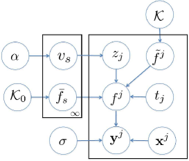
Figure 2: DPGMT: Plate graph

In this model, the concentration parameter $\alpha$ is assumed to be known. As in Equation (12), the inference task is to find the MAP estimates of the parameter set $\mathcal{M}=\{\{\bar{f}_{s}\},\{t_{j}\},\sigma^{2},\mathcal{K}\}$. Notice that in contrast with the previous model, the mixture proportion are not estimated here. To perform the inference, we must consider another set of hidden variables $\mathbf{v}=\{v_{i}\}$ in addition to $\mathbf{f}$ and $\mathbf{z}$. However, calculating the posterior of the hidden variables is intractable, thus the variational em algorithm (e.g., Bishop, 2006) is used to perform the approximate inference. The algorithm can be summarized as follows:

• Variational E-Step Choose a family $\mathcal{G}$ of variational distributions $q(\mathbf{f,v,z})$ and find the distribution $q^{*}$ that minimizes the Kullback-Leibler (KL) divergence between the posterior distribution and the proposed distribution given the current estimate of parameters, i.e.

  $$q^{*}(\mathbf{f,v,z};\mathcal{M}^{g})=\underset{q\in\mathcal{G}}{\text{argmin}}\ \text{{KL}}\left(q(\mathbf{f,v,z})||\Pr(\mathbf{f,v,z}|\mathcal{X,Y};\mathcal{M}^{g})\right)$$ (43)

  where

  $$\text{{KL}}\left(q(\mathbf{f,v,z})||\Pr(\mathbf{f,v,z}|\mathcal{X,Y};\mathcal{M}^{g})\right)=\int\log\left[\frac{q(\mathbf{f,v,z})}{\Pr(\mathbf{f,v,z}|\mathcal{X,Y};\mathcal{M}^{g})}\right]\text{d}q(\mathbf{f,v,z}).$$

• Variational M-Step Optimize the parameter set $\mathcal{M}$ such that

  $$\mathcal{M}^{*}=\underset{\mathcal{M}}{\text{argmax}}\ Q(\mathcal{M,M}^{g})$$

  where

  $$Q(\mathcal{M},\mathcal{M}^{g})={\rm I\!E}_{q^{*}(\mathbf{z,f,v};\mathcal{M}^{g})}\left[\log\left\{\Pr(\mathcal{Y},\mathbf{f,z,v}|\mathcal{X};\mathcal{M})\times\Pr[\{\bar{f}_{s}\};\mathcal{K}_{0}]\right\}\right].$$ (44)

Variational E-Step. For the variational distribution $q()$ we use the mean field approximation (Wainwright and Jordan, 2008). That is we assume a factorized distribution for disjoint group of random variables. This results in an analytic tractable optimization problem. In addition, following  (Blei and Jordan, 2006), we approximate the distribution over $\mathbf{v}$ using a truncated stick-breaking representations, where for a fix $T$, $q(v_{T}=1)=1$ and therefore $\pi_{s}(\mathbf{v})=0,\ s>T$. In this paper, we fix the truncation level $T$ while in general it can also be treated as a variational parameter. Concretely, we propose the following factorized family of variational distributions over the hidden variables $\{\mathbf{f,v,z}\}$:

$$q(\mathbf{f,v,z})=\prod_{s=1}^{T-1}q_{s}(v_{s})\prod_{j=1}^{M}q_{j}(f_{j},z_{j}).$$ (45)

Note that we do not assume any parametric form for $\{q_{s},q_{j}\}$ and our only assumption is that the distribution factorizes into independent components. To optimize Equation (43), recall the following result from (Bishop, 2006, Chapter 8):

Lemma 1

Suppose we are given a probabilistic model with a joint distribution $\Pr(\mathbf{X,Z})$ over $\mathbf{X,Z}$ where $\mathbf{X}=\{\mathbf{x}_{1},\mathbf{x}_{2},\cdots,\mathbf{x}_{N}\}$ denote the observed variables and all the parameters and hidden variables are $\mathbf{Z}=\{\mathbf{z}_{1},\mathbf{z}_{2},\cdots,\mathbf{z}_{M}\}$. Assume the distribution of $\mathbf{Z}$ has the following form:

$$q(\mathbf{Z})=\prod_{i}^{M}q_{i}(z_{i}).$$

Then, the KL divergence between the posterior distribution $\Pr(\mathbf{Z}|\mathbf{X})$ and $q(\mathbf{Z})$ is minimized and the optimal solution $q_{j}^{*}(\mathbf{z}_{j})$ is given by

$$q_{j}^{*}(\mathbf{z}_{j})\propto\text{exp}\left({\rm I\!E}_{i\neq j}\left[\log\Pr(\mathbf{X},\mathbf{Z})\right]\right)$$

where ${\rm I\!E}_{i\neq j}[\cdots]$ denotes the expectation w.r.t. $q()$ over all $Z_{j},\ j\neq i$.

From the graphical model in Figure 2, the joint distribution of $\Pr(\mathcal{Y},\mathbf{f,v,z}|\mathcal{X};\mathcal{M}^{g})$ can be written as:

$$\begin{split}\Pr(\mathcal{Y},\mathbf{f,v,z}|\mathcal{X})&=\Pr(\mathcal{Y}|\mathcal{X},\mathbf{f,z})\Pr(\mathbf{z}|\mathbf{v})\Pr(\mathbf{f}|\mathcal{X})\Pr(\mathbf{v}|\alpha)\\ &=\prod_{j}\Pr(\mathbf{y}^{j}|\mathbf{x}^{j},\mathbf{f}_{j},z_{j})\prod_{j}\Pr(z_{j}|\mathbf{v})\prod_{j}\Pr(\mathbf{f}_{j}|\mathbf{x}^{j})\prod_{s}\Pr(v_{s}|\alpha).\end{split}$$

Equivalently,

$$\begin{split}\log\Pr(\mathcal{Y},\mathbf{f,v,z}|\mathcal{X})&=\sum_{j}\log\Pr(\mathbf{y}^{j}|\mathbf{x}^{j},\mathbf{f}_{j},z_{j})\\ &\qquad+\sum_{j}\log\Pr(z_{j}|\mathbf{v})+\sum_{j}\log\Pr(\mathbf{f}_{j}|\mathbf{x}^{j})+\sum_{s}\log\Pr(v_{s}|\alpha).\end{split}$$

First we consider the distribution of $q_{s}(\mathbf{v})$. Following Blei and Jordan (2006), the second term can be expanded as

$$\log\Pr(z_{j}|\mathbf{v})=\sum_{t=1}^{T}\mathbbold{1}_{\{z_{j}>t\}}\log(1-v_{t})+\mathbbold{1}_{\{z_{j}=t\}}\log v_{t}$$ (46)

where $\mathbbold{1}$ is the indicator function. Therefore, using the lemma above and denoting $\mathbf{v}\backslash v_{s}$ by $\mathbf{v}_{-s}$, we have

$$\begin{split}\log q_{s}(v_{s})&\propto{\rm I\!E}_{\mathbf{z,f,v}_{-s}}\left[\log\Pr(\mathcal{Y},\mathbf{f,v,z}|\mathcal{X})\right]\\ &=\sum_{j}\left({\rm I\!E}_{\mathbf{z,f,v}_{-s}}[\mathbbold{1}_{\{z_{j}>s\}}]\log(1-v_{s})+{\rm I\!E}_{\mathbf{z,f,v}_{-s}}[\mathbbold{1}_{\{z_{j}=s\}}]\log v_{s}\right)+\log\Pr(v_{s}|\alpha)+\text{constant}\\ &=\sum_{j}\left(q(z_{j}>s)\log(1-v_{s})+q(z_{j}=s)\log v_{s}\right)+\log\Pr(v_{s}|\alpha)+\text{constant}\end{split}$$

Recalling that the prior is given by $\text{Beta}(1,\alpha)$ we see that the distribution of $q_{s}(v_{s})$ is

$$q_{s}(v_{s})\propto v_{s}^{\sum_{j}q(z_{j}=s)}(1-v_{s})^{\alpha+\sum_{j}\sum_{l=s+1}^{T}q(z_{j}=l)-1}.$$

Observing the form of $q_{s}(v_{s})$, we can see that it is a Beta distribution and $q_{t}(v_{t})\sim\text{Beta}(\gamma_{t,1},\gamma_{t,2})$ where

$$\begin{split}\gamma_{t,1}&=1+\sum_{j}q(z_{j}=t)\\ \gamma_{t,2}&=\alpha+\sum_{j}\sum_{l=s+1}^{T}q(z_{j}=l).\end{split}$$

We next consider $q_{j}(\mathbf{f}_{j},z_{j})$. Notice that we can always write $q_{j}(\mathbf{f}_{j},z_{j})=q_{j}(\mathbf{f}_{j}|z_{j})q_{j}(z_{j})$. Denote $h(z_{j})={\rm I\!E}_{\mathbf{v}}\left[\log\Pr(z_{j}|\mathbf{v})\right]$, then again using the lemma above we have

$$\begin{split}q_{j}(\mathbf{f}_{j}|z_{j})q_{j}(z_{j})&\propto e^{h(z_{j})}\Pr(\mathbf{y}^{j}|\mathbf{x}^{j},\mathbf{f}_{j},z_{j})\Pr(\mathbf{f}_{j}|\mathbf{x}^{j})\\ &=e^{h(z_{j})}\Pr(\mathbf{y}^{j},\mathbf{f}_{j}|\mathbf{x}^{j},z_{j})\\ &\propto e^{h(z_{j})}\Pr(\mathbf{y}^{j}|\mathbf{x}^{j},z_{j})\Pr(\mathbf{f}_{j}|\mathbf{x}^{j},\mathbf{y}^{j},z_{j})\\ &\propto\left[\underbrace{e^{h(z_{j})}\Pr(\mathbf{y}^{j}|\mathbf{x}^{j},z_{j})}_{q_{j}(z_{j})}\right]\left[\underbrace{\Pr(\mathbf{f}_{j}|\mathbf{x}^{j},\mathbf{y}^{j},z_{j})}_{q_{j}(\mathbf{f}_{j}|z_{j})}\right].\\ \end{split}$$

The equality in the second line holds because $\Pr(\mathbf{f}_{j}|\mathbf{x}^{j})=\Pr(\mathbf{f}_{j}|\mathbf{x}^{j},z_{j})$; their distributions become coupled when conditioned on the observations $\mathbf{y}^{j}$, but without such observations they are independent. Therefore the left term yields

$$q_{j}(z_{j})\propto e^{h(z_{j})}\Pr(\mathbf{y}^{j}|\mathbf{x}^{j},z_{j})$$

where $\Pr(\mathbf{y}^{j}|\mathbf{x}^{j},z_{j})$ is given by Equation (16). The value of $h(z_{j})$ can be calculated using Equation (46):

$$\begin{split}\log\Pr(z_{j}=s|\mathbf{v})&=\sum_{t=1}^{s-1}\log(1-v_{t})+\log v_{s}\\ h(z_{j}=s)&={\rm I\!E}_{v_{s}}[\log v_{s}]+\sum_{i=1}^{s-1}{\rm I\!E}_{v_{i}}\left[\log(1-v_{i})\right]\end{split}$$

where

$$\begin{split}{\rm I\!E}_{v_{t}}[\log v_{t}]&=\Psi(\gamma_{i,1})-\Psi(\gamma_{i,1}+\gamma_{i,2})\\ {\rm I\!E}_{v_{i}}\left[\log(1-v_{i})\right]&=\Psi(\gamma_{i,2})-\Psi(\gamma_{i,1}+\gamma_{i,2}).\end{split}$$

Consequently, $q_{j}(z_{j})$ has the following form

$$q_{j}(z_{j}=t)\propto\text{exp}\left\{{\rm I\!E}_{v_{t}}[\log v_{t}]+\sum_{i=1}^{t-1}{\rm I\!E}_{v_{i}}\left[(1-v_{i})\right]\right\}\times\mathcal{N}\left(\overline{\mathbf{f}}^{j},\mathbf{K}_{j}^{g}+\sigma^{2}\mathbb{I}\right).$$ (47)

Note that this is the same form as in Equation (15) of the previous model where $\Pr(z_{j};\mathcal{M}^{g})$ is replaced by $e^{h(z_{j}=t)}$.

Given $z_{j}$, $q_{j}(\mathbf{f}_{j}|z_{j})$ is identical to Equation (17) and leads to the conditional distribution such that

$$q_{j}(\mathbf{f}_{j}|z_{j})\propto\Pr(\mathbf{y}^{j}|\mathbf{x}^{j},\mathbf{f}_{j},z_{j})\Pr(\mathbf{f}_{j};\mathbf{x}^{j})$$

which is the posterior distribution under GP regression and thus is exactly the same form as in the previous model.

Variational M-Step. Denote $\widetilde{Q}$ as the expectation of the complete data log likelihood w.r.t. the hidden variables. Then as in Equation (20), we have

$$\begin{split}\widetilde{Q}&={\rm I\!E}_{q(\mathbf{v})}{\rm I\!E}_{q(\mathbf{z})}{\rm I\!E}_{q(\mathbf{f}|\mathbf{z})}\log\left(\prod_{j}\prod_{s}\left[\pi_{s}(\mathbf{v})\Pr(\mathbf{y}^{j}|\mathbf{f}_{j},z_{j}=s;\mathcal{M})\Pr(\mathbf{f}_{j};\mathcal{M})\right]^{z_{js}}\right)\\ &={\rm I\!E}_{\mathbf{v}}\Bigg{[}\sum_{\mathbf{z}}q(\mathbf{z})\Bigg{\{}\sum_{j}\sum_{s}z_{js}\cdot\int dq(\mathbf{f}_{j}|z_{j}=s)\\ &\qquad\times\log\left[\pi_{s}(\mathbf{v})\Pr(\mathbf{y}^{j}|\mathbf{f}_{j},z_{j}=s;\mathcal{M})\Pr(\mathbf{f}_{j};\mathcal{M})\right]\Bigg{\}}\Bigg{]}\\ &=\sum_{\mathbf{z}}q(\mathbf{z})\Bigg{\{}\sum_{j}\sum_{s}z_{js}\cdot\int dq(\mathbf{f}_{j}|z_{j}=s)\\ &\qquad\times\log\left[\Pr(\mathbf{y}^{j}|\mathbf{f}_{j},z_{j}=s;\mathcal{M})\Pr(\mathbf{f}_{j};\mathcal{M})\right]\Bigg{\}}+{\rm I\!E}_{\mathbf{v}}\left[\sum_{j}\sum_{s}\log\pi_{s}(\mathbf{v})\right].\end{split}$$ (48)

Notice that ${\rm I\!E}_{\mathbf{v}}\left[\sum_{j}\sum_{s}\log\pi_{s}(\mathbf{v})\right]$ is a constant w.r.t.  the parameters of $\mathcal{M}$ and can be dropped in the optimization. Thus, following the same derivation as in the GMT model, we have the form of the $Q$ function as

$$\begin{split}Q(\mathcal{M},\mathcal{M}^{g})&=-\frac{1}{2}\sum_{s}\|\bar{f}_{s}\|_{\mathcal{H}_{0}}^{2}-\sum_{j}n_{j}\log\sigma\\ &\qquad-\frac{1}{2\sigma^{2}}\sum_{j}\sum_{s}\gamma_{js}{\rm I\!E}_{\{q(\mathbf{f}_{j}|z_{j}=s)\}}\left[\|\mathbf{y}^{j}-[\bar{f}_{s}*\delta_{t_{j}}](\mathbf{x}^{j})-\mathbf{f}_{j}\|^{2}\right]\\ &\qquad+\sum_{j}\sum_{s}\gamma_{js}{\rm I\!E}_{\{q(\mathbf{f}_{j})\}}\left[\log\Pr(\mathbf{f}_{j};\mathcal{M})\right].\end{split}$$ (49)

where $\gamma_{js}$ is given by Equation (22). Now because the $q_{j}(z_{j})$ and $q_{j}(f_{j}|z_{j})$ have exactly the same form as before (except $\Pr(z_{j};\mathcal{M}^{g})$ is replaced by Equation (47)), the previous derivation of the M-Step w.r.t. the parameter set $\mathcal{M}$ still holds.

To summarize, the algorithm is the same as Algorithm 1 except that

• we drop step 6,

• we add a step between steps 3 and 4 calculating $\gamma_{i,1}$ and $\gamma_{i,2}$ using Equation 5.2,

• step 4 calculating Equation (22) uses Equation (47) instead of Equation (15).

6 Experiments

Our implementation of the algorithm makes use of the gpml package (Rasmussen and Nickisch, 2010) and extends it to implement the required functions. The em algorithm is restarted 5 times and the function that best fits the data is chosen. The em algorithm stops when difference of the log-likelihood is less than 10e-5 or at a maximum of 200 iterations.

6.1 Regression on Synthetic data

In the first experiment, we demonstrate the performance of our algorithm on a regression task with artificial data. We generated the data following Assumption 1 under a mixture of three Gaussian processes. More precisely, each $\bar{f}_{s}(x),s=1,2,3$ is generated on the interval $[-50,50]$ from a Gaussian process with covariance function

$$\text{cov}[\bar{f}_{s}(t_{1}),\bar{f}_{s}(t_{2})]=e^{-\frac{(t_{1}-t_{2})^{2}}{25}},\quad s=1,2,3.$$

The individual effect $\tilde{f}_{j}$ is sampled via a Gaussian process with the covariance function

$$\text{cov}[\tilde{f}_{j}(t_{1}),\tilde{f}_{j}(t_{2})]=0.2e^{-\frac{(t_{1}-t_{2})^{2}}{16}}.$$

Then the hidden label $z_{j}$ is sampled from a discrete distribution with the parameter $\alpha=[0.5,0.5]$. The vector $\breve{\mathbf{x}}$ consists of 100 samples on $[-50,50]$. We fix a sample size $N$, each $\mathbf{x}^{j}$ includes $N$ randomly chosen points from $\{\breve{x}_{1},\cdots,\breve{x}_{100}\}$ and the observation $f^{j}(\mathbf{x}^{j})$ is obtained as $(f_{z_{j}}+\tilde{f}_{j})(\mathbf{x}^{j})$. In the experiment, we vary the individual sample length $N$ from 5 to 50. Finally, we generated 50 random tasks with the observation $\mathbf{y}^{j}$ for task $j$ given by

$$\mathbf{y}^{j}\sim\mathcal{N}(f^{j}(\mathbf{x}^{j}),0.01\times\mathbb{I}),\quad j=1,\cdots,50.$$

The methods compared here include

1. Single-task learning procedure (ST), where each $\bar{f}^{j}$ is estimated only using $\{\mathbf{x}^{j}_{i},\mathbf{y}^{j}_{i}\},i=1,2,\cdots,N$.

2. Single center mixed-effect multi-task learning (SCMT), amounts to the mixed-effect model (Pillonetto et al., 2010) where one average function $\bar{f}$ is learned from $\{\mathbf{x}^{j},\mathbf{y}^{j}\},j=1,\cdots,50$ and $f^{j}=\bar{f}+\tilde{f}^{j},j=1,\cdots,50$.

3. Grouped mixed-effect model (GMT), the proposed method with number of clusters fixed to be the true model order.

4. Dirichlet process Grouped mixed-effect model (DP-GMT), the infinite mixture extension of the proposed model.

5. “Cheating” grouped fixed-effect model (CGMT), which follows the same algorithm as the grouped mixed-effect model but uses the true label $z_{j}$ instead of their expectation for each task $j$. This serves as an upper bound for the performance of the proposed algorithm.

All algorithms (except for ST which does not estimate the kernel of the individual variations) use the same method to learn the kernel of the individual effects, which is assumed to have the form

$$\text{cov}[\tilde{f}_{j}(t_{1}),\tilde{f}_{j}(t_{2})]=ae^{-\frac{(t_{1}-t_{2})^{2}}{s^{2}}}.$$

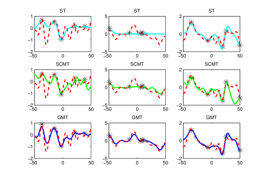
Figure 3: Simulated data: Comparison of the estimated function between single, multi-task and grouped multi-task. The red dotted line is the reference true function.

The Root Mean Square Error (RMSE) for the four approaches is reported. For task $j$, the RMSE is defined as

$$\text{RMSE}_{j}=\sqrt{\frac{1}{100}\|f(\breve{\mathbf{x}})-f^{j}(\breve{\mathbf{x}})\|^{2}}$$

where $f$ is the learned function and RMSE for the data set is the mean of $\{\text{RMSE}_{j}\},j=1,\cdots,50$. To illustrate the results qualitatively, we first plot in Figure 3 the true and learned functions in one trial. The left/center/right column illustrates some task that is sampled from group effect $\bar{f}_{1}$, $\bar{f}_{2}$ and $\bar{f}_{3}$. It it easy to see that, as expected, the tasks are poorly estimated under ST due the sparse sampling. The SCMT performs better than ST but its estimate is poor in areas where the three centers disagree. The estimates of GMT are much closer to the true function.

Figure 4 shows a comparison of the algorithms for 50 random data sets under the above setting when $N$ equals 5. We see that GMT with the correct model order $k=3$ almost always performs as well as its upper bound, illustrating that it recovers the correct membership of each task. On only three data sets, our algorithm is trapped in a local maximum yielding performance similar to SCMT and ST. Figure 5 shows the RMSE for increasing values of $N$ for the same experimental setup. From the plot we can draw the conclusion that the proposed method works much better than SCMT and ST when the number of samples is less than 30. As the number of samples for each task increases, all methods are improving, but the proposed method always outperforms SCMT and ST in our experiments. Finally, all algorithms converge to almost the same performance level where observations in each task are sufficient to recover the underlying function. Finally, Figure 5 also includes the performance of the DP-GMT on the same data. The truncation level of the Dirichlet process is 10 and the concentration parameter $\alpha$ is set to be 1. As we can see the DP-GMT is not distinguishable from the GMT (which has the correct $k$), indicating that the model selection is successful in this example.

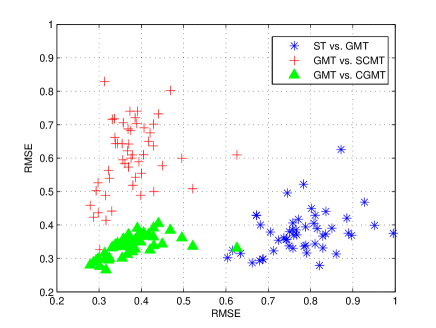
Figure 4: Simulated data: Comparison between single, multi-task, and grouped multi-task when sample size is 5. The figure gives 3 pairwise comparison. The Blue stars denote ST vs. GMT: we can see the GMT is better than ST since the stars are concentrated on the lower right. Similarly, the plot of red pluses demonstrates the advantage of GMT over SCMT and the plot of green triangles shows that the algorithm behaves almost as well as its upper bound.

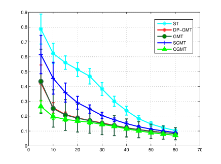
Figure 5: Simulated data: Performance comparison of single, multi-task, and grouped multi-task, and DP grouped multi-task as a function of the number of samples per task.

6.2 Classification on Astrophysics data

The concrete application motivating this research is the classification of stars into several meaningful categories from the astronomy literature. Classification is an important step within astrophysics research, as evidenced by published catalogs such as OGLE (Udalski et al., 1997) and MACHO (Alcock et al., 1993; Faccioli et al., 2007). However, the number of stars in such surveys is increasing dramatically. For example Pan-STARRS (Hodapp et al., 2004) and LSST (Starr et al., 2002) collect data on the order of hundreds of billions of stars. Therefore, it is desirable to apply state-of-art machine learning techniques to enable automatic processing for astrophysics data classification.

The data from star surveys is normally represented by time series of brightness measurements, based on which they are classified into categories. Stars whose behavior is periodic are especially of interest in such studies. Figure 6 shows several examples of such time series generated from the three major types of periodic variable stars: Cepheid, RR Lyrae, and Eclipsing Binary. In our experiments only stars of these classes are present in the data, and the period of each star is given.

Figure 6: Examples of light curves of periodic variable stars. Each column shows two stars of the same type. Left: Cepheid, middle: RR Lyrae, right: eclipsing binary.

From Figure 6, it can be noticed that there are two main characteristics of this data set:

• The time series are not phase aligned, meaning that the light curves in the same category share a similar shape but with some unknown shift.

• The time series are non-synchronously sampled and each light curve has different number of samples and sampling times.

We run our experiment on the OGLEII data set (Soszynski et al., 2003). This data set consists of 14087 time series from periodic variable stars with 3425 Cepheids, 3390 EBs and 7272 RRLs. We use the time series measurements in the I band  (Soszynski et al., 2003). We perform several experiments with this data set to explore the potential of the proposed method. In previous work with this dataset Wachman et al. (2009) developed a kernel for periodic time series and used it with svm to obtain good classification performance. We use the results of Wachman et al. (2009) as our baseline.

6.2.1 Classification using dense-sampled time series

In the first experiment, the time series are smoothed using a simple average filter, re-sampled to 50 points via linear-interpolation and normalized to have mean 0 and standard deviation of 1. Therefore, the time series are synchronously sampled in the pre-processing. We compare our method to Gaussian mixture model (GMM) and 1-Nearest Neighbor (1-NN). These two approaches are performed on the time series processed by Universal phasing (UP), which uses the method from Protopapas et al. (2006) to phase each time series according to the sliding window on the time series with the maximum mean. We use a sliding window size of $5\%$ of the number of original points; the phasing takes place after the pre-processing explained above. We learn a separate model for each class and for each class the model order for GMM and GMT is set to be 15.

	up $+$ gmm	gmt	up $+$ 1-nn	k $+$ svm
Results	$0.956\pm 0.006$	$0.952\pm 0.005$	$0.865\pm 0.006$	$0.947\pm 0.005$

Table 1: Accuracies with standard deviations reported on OGLEII dataset.

We run 10-fold cross-validation (CV) over the entire data set and the results are shown in Table 1. We see that when the data is densely and synchronously sampled, the proposed method performs similar to the GMM, and they both outperform the kernel based results of Wachman et al. (2009). The similarity of the GMM and the proposed method under these experimental conditions is not surprising. The reason is that when the time series are synchronously sampled, aside from the difference of phasing, finding the group effect functions is reduced to estimating the mean vectors of the GMM. In addition, learning the kernel in the non-parametric approach is equivalent to estimating the covariance matrix of the GMM. More precisely, assuming all time series are phased (that is, $t_{j}=0$ for all $j$), the following results hold:

1. By placing a flat prior on the group effect function $\bar{f}_{s},s=1,\cdots,k$, or equivalently setting $\|\bar{f}_{s}\|^{2}_{\mathcal{H}_{0}}=0$, Equation (28) is reduced to finding a vector $\mu_{s}\in{\rm I\!N}$ that minimizes $\sum_{j}\gamma_{js}\|\tilde{\mathbf{y}}^{j}-\mu_{s}\|^{2}$. Therefore, we obtain $\bar{f}_{s}=\mu_{s}=\sum_{j}\gamma_{js}\tilde{\mathbf{y}}_{j}/\sum_{j}\gamma_{js}$, which is exactly the mean of the $s$th cluster during the iteration of em algorithm under the GMM setting.

2. The kernel $\mathbf{K}$ is learned in a non-parametric way. For the GP regression model, we see that considering noisy observations is essentially equivalent to considering non-noisy observations, but slightly modifying the model by adding a diagonal term on the covariance function for $\mathbf{f}_{j}$. Therefore, instead of estimating $\mathbf{K}$ and $\sigma^{2}$, it is convenient to put these two terms together, forming $\widehat{\mathbf{K}}=\mathbf{K}+\sigma^{2}\mathbb{I}$. In other words, we add a $\sigma^{2}$ term to the variance of $\mathbf{f}_{j}$ and remove it from $\mathbf{y}^{j}$ which becomes deterministic. In this case, comparing to the derivation in Equation (16)—(19) we have $\mathbf{f}_{j}=\mathbf{y}^{j}-\mathbf{\bar{f}}^{j}$ and $\mathbf{f}_{j}$ is determined given $z_{j}$. Comparing to Equation (17) we have the posterior mean $\boldsymbol{\mu}_{js}^{g}=\widehat{\mathbf{K}}\widehat{\mathbf{K}}^{-1}(\mathbf{y}^{j}-\mu_{s})=\mathbf{y}^{j}-\mu_{s}$ and the posterior covariance matrix $\mathbf{C}_{j}^{g}$ vanishes. Applying these values in Equation (40) we get $\widehat{\mathbf{K}}=\frac{1}{M}\sum_{j}\sum_{s}\gamma_{js}(\mathbf{y}^{j}-\mu_{s})(\mathbf{y}^{j}-\mu_{s})^{\mathrm{T}}$. In the standard em algorithm for the GMM, this is equal to the estimated covariance matrix when all $k$ clusters are assumed to have the same variance.

Accordingly, when time series are synchronously sampled, the proposed model can be viewed as an extension of the Phased K-means (Rebbapragada et al., 2009). The Phased K-means (PKmeans) re-phases the time series before the similarity calculation and updates the centroids using the phased time series. Therefore, with shared covariance matrix, our model is a shift-invariant (Phased) GMM and the corresponding learning process is a Phased em algorithm where each time series is re-phased in the E step. In experiments presented below we use Phased GMM directly in the feature space and generalize it so that each class has a separate covariance matrix.

We use the same experimental data to investigate the performance of the DP-GMT where the truncation level is set to be 30 and the concentration parameter $\alpha$ of the DP is set to be 1. The results are shown in Figure 7 and Table 2 where BIC-GMT means that the model order is chosen by BIC where the optimal $k$ is chosen from 1 to 30. The poor performance of SCMT shows that a single center is not sufficient for this data. As evident from the graph the DP-GMT is not distinguishable from the BIC-GMT. The advantage of the DP model is that this equivalent performance is achieved with much reduced computational cost because the BIC procedure must learn many models and choose among them whereas the DP learns a single model.

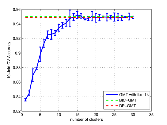
Figure 7: OGLEII data: Comparison of model selection methods using dense sampled data. The plot shows the performance of GMT with varying $k$, BIC for the GMT model, and DP-GMT. For visual clarity we only include the standard deviations on the GMT plot.

	scmt	gmt	dp-gmt	bic-gmt
Results	$0.874\pm 0.008$	$0.952\pm 0.005$	$0.949\pm 0.005$	$0.950\pm 0.002$

Table 2: Accuracies with standard deviations reported on OGLEII dataset.

6.2.2 Classification using sparse-sampled time series

The OGLEII data set is in some sense a “nice” subset of the data from its corresponding star survey. Stars with small number of samples are often removed in pre-processing steps. For example, Wachman (2009) developed full system to process the MACHO catalog and applied the kernel method to classify stars. In its pipeline, part of the preprocessing rejected 3.6 million light curves of the approximate 25 million because of insufficient number of observations. The proposed method potentially provides a way to include these instances in the classification process. In the second experiment, we demonstrate the performance of the proposed method on times series with sparse samples. Similar to the synthetic data, we started from sub-sampled versions of the original time series to simulate the condition that we would encounter in further star surveys. As in the previous experiment, each time series is universally phased, normalized and linearly-interpolated to length 50 to be plugged into GMM and 1-NN as well as the phased GMM mentioned above. The RBF kernel is used for the proposed method and we use model order 15 as above. Moreover, the performance for PKmeans is also presented, where the classification step is as follows: we learn the PKmeans model with $k=15$ for each class and then the label of a new example is assigned to be the same as its closest centroid’s label. PKmeans is also restarted 5 times and the best clustering is used for classification.

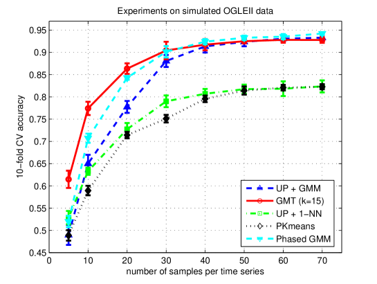
Figure 8: OGLEII data: Comparison of algorithms with sparsely sampled data

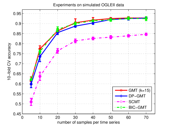
Figure 9: OGLEII data: Comparison of algorithms with sparsely sampled data

The results are shown in Figure 8. As can be easily observed, when each time series has sparse samples (i.e., number of samples per task is less than 30), the proposed method has a significant advantage over the other methods. As the number of samples per task increases, the proposed method improves fast and performs close to its optimal performance given by previous experiment. Three additional aspects that call for discussion can be seen in the figure. First, note that for all three methods, the performance with dense data is lower than results in Table 1. This can be explained by fact that the data set obtained by the interpolation of the sub-sampled measurements contains less information than that interpolated from the original measurements. Second, notice that the Phased em algorithm always outperforms the GMM plus UP demonstrating that re-phasing the time series inside the em algorithm improves the results. Third, when the number of samples increases, the performance of the Phased em gradually catches up and becomes better than the proposed method when each task has more than 50 samples. GMM plus universal phasing (UP) also achieves better performance when time series are densely sampled. One reason for the performance difference is the difference in the way the kernel is estimated. In Figure 8 GMT uses the parametric form of the kernel which is less expressive than getting precise estimates for every $\mathcal{K}(t_{1},t_{2})$. The GMM uses the non-parametric form which, given sufficient data, can lead to better estimates. A second reason can be attributed to the sharing of the covariance function in our model where the GMM and the Phased GMM do not apply this constraint.

Finally, we use the same experimental setting to compare the performance of various mode selection models. The results are shown in Figure 9. The performance of BIC is not distinguishable from the optimal $k$ selected in hindsight. The performance of DP is slightly lower but it comes close to these models.

To summarize, we conclude from the experiments with astronomy data that Phased em is appropriate with densely sampled data but that the GMT and its variants should be used when data is sparsely and non-synchronously sampled. In addition BIC coupled with GMT performs excellent model selection and DP does almost as well with a much reduced computational complexity.

6.2.3 Class discovery:

We show the potential of our model for class discovery by running two version of the GMT model on the joint data set of the three classes (not using the labels). Then, each cluster is labeled according to the majority class of the instances that belong to the center. For a new test point, we determine which cluster it belongs to via the MAP probability and its label is given by the cluster that it is assigned to. We run 10 trials with different random initializations. In accordance with previous experiments that used 15 components per class we run GMT with model order of 45. We also run DP-GMT with a truncation level set to 90. The GMT obtains accuracy and standard deviation of $[0.895,0.010]$ and the DP models obtains accuracy and standard deviation of $[0.925,0.013]$. Note that it is hard to compare between the results because of the different model orders used. Rather than focus on the difference, the striking point is that we obtain almost pure clusters without using any label information. Given the size of the data set and the relatively small number of clusters this is a significant indication of the potential for class discovery in astrophysics.

7 Related Work

Classification of time series has attracted an increasing amount of interest in recent years due to its wide range of potential applications, for example ECG diagnosis (Wei and Keogh, 2006), EEG diagnosis (Lu et al., 2008), and Speech Recognition (Povinelli et al., 2004). Common methods choose some feature based representation or distance function for the time series (for example the sampled time points, or Fourier or wavelet coefficients as features and dynamic time warping for distance function) and then apply some existing classification method  (Osowski et al., 2004; Ding et al., 2008). Our approach falls into another category, that is, model-based classification where the time series are assumed to be generated by a probabilistic model and examples are classified using maximum likelihood or MAP estimates. A family of such models, closely related to the GMT, is discussed in detail below. Another common approach uses Hidden Markov models as a probabilistic model for sequence classification, and this has been applied to time series as well (Kim and Smyth, 2006).

Learning Gaussian processes from multiple tasks has previously been investigated in the the hierarchical Bayesian framework, where a group of related tasks are assumed to share the same prior. Under this assumption, training points across all tasks are utilized to learn a better covariance function via the em algorithm (Yu et al., 2005; Schwaighofer et al., 2005). In addition, Lu et al. (2008) extended the work of Schwaighofer et al. (2005) to a non-parametric mixed-effect model where each task can have its own random effect. Our model is based on the same algorithmic approach where the values of the function for each task at its corresponding points (i.e. $\{\mathbf{f}_{j}\}$ in our model) are considered as hidden variables. Furthermore, the proposed model is a natural generalization of Schwaighofer et al. (2005) where the fixed-effect function is sampled from a mixture of regression functions each of which is a realization of a common Gaussian process. Along a different dimension, our model differs from the infinite mixtures of Gaussian processes model for clustering (Jackson et al., 2007) in two aspects: first, instead of using zero mean Gaussian process, we allow the mean functions to be sampled from another Gaussian process; second, the individual variation in our model serves as the covariance function in their model but all mixture components share the same kernel.

Although having a similar name, the Gaussian process mixture of experts model focuses mainly on the issues of non-stationarity in regression (Rasmussen and Ghahramani, 2002; Tresp, 2001). By dividing the input space into several (even infinite) regions via a gating network, the Gaussian process mixture of expert model allows different Gaussian processes to make predictions for different regions.

In terms of the clustering aspect, our work is most closely related to the so-called mixture of regressions (Gaffney and Smyth, 2005, 2003; Gaffney, 2004; Gaffney and Smyth, 1999). The name comes from the fact that these approaches substitute component density models with conditional regression density models in the framework of standard mixture model. For phased time series, Gaffney and Smyth (1999) first proposed the regression-based mixture model where they used Polynomial and Kernel regression models for the mean curves. Further, Gaffney and Smyth (2003) integrated the linear random effects models with mixtures of regression functions. In their model, each time series is sampled by a parametric regression model whose parameters are generated from a Gaussian distribution. To incorporate the time shifts, Chudova et al. (2003) proposed a shift-invariant Gaussian mixture model for multidimensional time series. They constrained the covariance matrices to be diagonal to handle the non-synchronous case. They also treated time shifts as hidden variables and derived the em algorithm under full Bayesian settings, i.e. where each parameter has a prior distribution. Furthermore, Gaffney and Smyth (2005) developed a generative model for misaligned curves in a more general setting. Their joint clustering-alignment model also assumes a normal parametric regression model for the cluster labels, and Gaussian priors on the hidden transformation variables which consist of shifting and scaling in both the time and magnitude. Our model extends the work of Gaffney and Smyth (2003) to admit non-parametric Bayesian regression mixture models and at the same time handle the non-phased time series. If the group effects are assumed to have a flat prior, our model differs from Chudova et al. (2003) in the following two aspects in addition to the difference of Bayesian treatment. First, our model does not include the time shifts as hidden variables but instead estimates them as parameters. Second, we can handle shared full covariance matrix instead of diagonal ones by using a parametric form of the kernel. On the other hand, given the time grid $\breve{\mathbf{x}}$, we can design the kernel for individual variations as $\mathcal{K}(\breve{x}_{i},\breve{x}_{j})=a_{i}\delta_{ij}(\breve{x}_{i},\breve{x}_{j}),i,j=1,\cdots,{\rm I\!N}$. Using this choice, our model is the same as Chudova et al. (2003) with shared diagonal covariance matrix. In summary, our model allows a more flexible structure of the covariance matrix that can treat synchronized and non-synchronized time series in a unified framework, but at the same time it is constrained to have the same covariance matrix across all clusters.

8 Conclusion

We developed a novel Bayesian nonparametric multi-task learning model (GMT) where each task is modeled as a sum of a group-specific function and an individual task function with a Gaussian process prior. We also extended the model such that the number of groups is not bounded using a Dirichlet process mixture model (DP-GMT). We derive efficient em and variational em algorithms to learn the parameters of the models and demonstrated their effectiveness using experiments in regression, classification and class discovery. Our models are particularly useful for sparsely and non-synchronously sampled time series data, and model selection can be effectively performed with these models.

There are several natural directions for future work. For application in the astronomy context it is important to consider all steps of processing and classification of a new sky survey so as to provide an end to end system. Therefore, two important issues to be addressed in future work include incorporating the period estimation phase into the method and developing an appropriate method for abstention in the classification step. It would also be interesting to develop a corresponding discriminative model extending Xue et al. (2007) to the GP context. Finally, one of the drawbacks of the GP based methods is the computational complexity which is too high for large scale problems. For example, in the experiments on sparse OGLEII data, we had to resample the data on a fine grid to avoid performing Cholesky decomposition for high dimensional matrices. Therefore, an important direction for future work is to find non-trivial sparse GP approximations that yield good performance with the GMT model.

Acknowledgments

This research was partly supported by NSF grant IIS-0803409. The experiments in this paper were performed on the Odyssey cluster supported by the FAS Research Computing Group at Harvard and the Tufts Linux Research Cluster supported by Tufts UIT Research Computing.

References

- Alcock et al. (1993) C. Alcock et al. The MACHO Project - a Search for the Dark Matter in the Milky-Way. In B. T. Soifer, editor, Sky Surveys. Protostars to Protogalaxies, volume 43 of Astronomical Society of the Pacific Conference Series, pages 291–296, 1993.
- Bi et al. (2008) J. Bi, T. Xiong, S. Yu, M. Dundar, and R. Rao. An improved multi-task learning approach with applications in medical diagnosis. European Conference on Machine Learning and Knowledge Discovery in Databases, pages 117–132, 2008.
- Bickel et al. (2008) S. Bickel, J. Bogojeska, T. Lengauer, and T. Scheffer. Multi-task learning for HIV therapy screening. In Proceedings of the 25th international conference on Machine learning, pages 56–63. ACM, 2008.
- Bishop (2006) C.M. Bishop. Pattern recognition and machine learning, volume 4. Springer New York, 2006.
- Blei and Jordan (2006) D.M. Blei and M.I. Jordan. Variational inference for Dirichlet process mixtures. Bayesian Analysis, 1(1):121–144, 2006.
- Chudova et al. (2003) D. Chudova, S. J. Gaffney, E. Mjolsness, and P. Smyth. Translation-invariant mixture models for curve clustering. In Proceedings of the ninth ACM SIGKDD international conference on Knowledge discovery and data mining, pages 79–88. ACM, 2003.
- Dempster et al. (1977) A. P. Dempster, N. M. Laird, and D. B Rubin. Maximum-likelihood from incomplete data via the EM algorithm. Journal of the Royal Statistical Society, B39:1–38, 1977.
- Ding et al. (2008) H. Ding, G. Trajcevski, P. Scheuermann, X. Wang, and E. Keogh. Querying and mining of time series data: experimental comparison of representations and distance measures. Proceedings of the VLDB Endowment archive, 1(2):1542–1552, 2008.
- Dinuzzo et al. (2008) F. Dinuzzo, G. Pillonetto, and G. De Nicolao. Client-server multi-task learning from distributed datasets. Arxiv preprint arXiv:0812.4235, 2008.
- Evgeniou et al. (2000) T. Evgeniou, M. Pontil, and T. Poggio. Regularization networks and support vector machines. Advances in Computational Mathematics, 13(1):1–50, 2000.
- Evgeniou et al. (2006) T. Evgeniou, C.A. Micchelli, and M. Pontil. Learning multiple tasks with kernel methods. Journal of Machine Learning Research, 6(1):615–637, 2006.
- Faccioli et al. (2007) L. Faccioli, C. Alcock, K. Cook, G. E. Prochter, P. Protopapas, and D. Syphers. Eclipsing Binary Stars in the Large and Small Magellanic Clouds from the MACHO Project: The Sample. Astronomy Journal, 134:1963–1993, 2007.
- Gaffney (2004) S. J. Gaffney. Probabilistic curve-aligned clustering and prediction with regression mixture models. PhD thesis, University of California, Irvine, 2004.
- Gaffney and Smyth (1999) S. J. Gaffney and P. Smyth. Trajectory clustering with mixtures of regression models. In Proceedings of the fifth ACM SIGKDD international conference on Knowledge discovery and data mining, pages 63–72. ACM, 1999.
- Gaffney and Smyth (2003) S. J. Gaffney and P. Smyth. Curve clustering with random effects regression mixtures. In Proceedings of the Ninth International Workshop on Artificial Intelligence and Statistics, 2003.
- Gaffney and Smyth (2005) S. J. Gaffney and P. Smyth. Joint probabilistic curve clustering and alignment. Advances in neural information processing systems, 17:473–480, 2005.
- Gelman (2004) A. Gelman. Bayesian data analysis. CRC press, 2004.
- Hodapp et al. (2004) K. W. Hodapp et al. Design of the Pan-STARRS telescopes. Astronomische Nachrichten, 325:636–642, 2004.