Abstract

We study the problem of estimating the leading eigenvectors of a high-dimensional population covariance matrix based on independent Gaussian observations. We establish a lower bound on the minimax risk of estimators under the $l_{2}$ loss, in the joint limit as dimension and sample size increase to infinity, under various models of sparsity for the population eigenvectors. The lower bound on the risk points to the existence of different regimes of sparsity of the eigenvectors. We also propose a new method for estimating the eigenvectors by a two-stage coordinate selection scheme.

Keywords : minimax risk, high-dimensional data, principal component analysis, sparsity, spiked covariance model

1 Introduction

Principal components analysis (PCA) is a widely used technique in reducing dimensionality of multivariate data. A traditional setting where PCA is applicable involves repeated observations from a multivariate normal distribution. Two key theoretical questions are: i) what is the relation between the sample eigenvectors and the population ones ? and ii) how well can population eigenvectors be estimated under various sparsity assumptions ? When the dimension $N$ of the observations is fixed and the sample size $n$ increases to infinity, the asymptotic properties of the sample eigenvalues and eigenvectors are well-known [Anderson, 1963, Muirhead, 1982]. Most of this asymptotic analysis is based on the fact that the sample covariance approximates well the population covariance when the sample size is large. However, it is increasingly common to encounter statistical problems where the dimensionality of the observations is of the same order of magnitude as (or even bigger than) the sample size. In such cases, the sample covariance matrix, in general, is not a reliable estimate of the population covariance matrix.

To overcome this curse of dimensionality, several works studied the estimation of the population covariance matrix, under various models of sparsity. These include the development of banding and thresholding schemes Bickel and Levina [2008a, b], El Karoui [2008], Rothman et al. [2009], Cai and Liu [2011], and analysis of their rate of convergence in the spectral norm. More recent works, such as Cai et al. [2010] and Cai and Zhou [2011] established the minimax rate of convergence under the matrix $l_{1}$ norm and the spectral norm, and its dependence on the assumed sparsity level.

In contrast to these works, that studied estimation of the population covariance matrix, in this paper we consider a related but different problem, namely, the estimation of its leading eigenvectors. The interest in comparing these two problems is partially due to the fact that, when the population covariance is a low rank perturbation of the identity, which is a primary focus of this paper, sparsity of the eigenvectors corresponding to the non-unit eigenvalues implies sparsity of the whole covariance. Note that consistency of an estimator of the whole covariance matrix also implies convergence of its leading eigenvalues to their population counterparts. If the gaps between the neighboring distinct eigenvalues remain bounded away from zero, it also implies convergence of the corresponding eigen-subspaces El Karoui [2008]. Moreover, for population eigenvalues with multiplicity one and gaps with neighboring eigenvalues bounded away from zero, the upper bounds for the whole covariance estimation under the spectral norm, derived in Bickel and Levina [2008b] and Cai and Zhou [2011], also yield an upper bound on the rate of convergence of the corresponding eigenvectors under the $l_{2}$ loss. These works, however, did not study the following fundamental problem, considered in this paper: How well can the leading eigenvectors be estimated, namely, what are the minimax rates for eigenvector estimation ?

We formulate this eigenvector estimation problem under the well-studied “spiked population model” which assumes that

• the eigenvalues of the population covariance matrix $\Sigma$ are

  $$\lambda_{1}+\sigma^{2},\ldots,\lambda_{M}+\sigma^{2},\sigma^{2},\ldots,\sigma^{2},$$

  for some $M\geq 1$, where $\sigma^{2}>0$ and $\lambda_{1}>\lambda_{2}>\cdots>\lambda_{M}>0$.

This is a standard model in several scientific fields, including for example array signal processing (e.g. see van Trees [2002]) where the observations are modeled as the sum of an $M$-dimensional random signal and an independent, isotropic noise. It also arises as a latent variable model for multivariate data, for example in factor analysis [Jolliffe, 2002, Tipping and Bishop, 1998]. The assumption that the leading $M$ eigenvalues are distinct is made to simplify the analysis, as it ensures that the corresponding eigenvectors are identifiable up to a sign change. The assumption that all remaining eigenvalues are equal is not crucial as our analysis can be generalized to the case when these are only bounded by $\sigma^{2}$. Asymptotic properties of the eigenvalues and eigenvectors of the sample covariance matrix under this model, in the setting when $N/n\to c\in(0,\infty)$ as $n\to\infty$, have been studied by Baik and Silverstein [2006], Nadler [2008], Onatski [2006] and Paul [2007], among others. A conclusion of these studies is that when $N/n\to c>0$, the eigenvectors of standard PCA are inconsistent estimators of the population eigenvectors.

In analogy to the sparse covariance estimation setting, several works considered various models of sparsity for the leading eigenvectors and developed improved sparse estimators. For example Witten and Tibshirani [2009] and Zou et al. [2006], among others, imposed $l_{1}$-type sparsity constraints directly on the eigenvector estimates and proposed optimization procedures for obtaining them. Shen and Huang [2008] suggested a regularized low rank approach to sparse PCA. The consistency of the resulting leading eigenvectors was recently proven in Shen et al. [2011], using a formulation of sparsity in which the sample size $n$ is fixed while $N\to\infty$. d’Aspremont et al. [2008] suggested a semi-definite programming (SDP) problem as a relaxation to the $l_{0}$-penalty for sparse $\Sigma$. Assuming a single spike, Amini and Wainwright [2008] studied the asymptotic properties of the leading eigenvector of the covariance estimator obtained by d’Aspremont et al. [2008], in the joint limit as both sample size and dimension tend to infinity. Specifically, Amini and Wainwright [2008] considered a leading eigenvector with exactly $k\ll N$ nonzero entries all of the form $\{-1/\sqrt{k},1/\sqrt{k}\}$. For this hardest subproblem in the $k$-sparse $l_{0}$-ball, Amini and Wainwright [2008] first derived information theoretic lower bounds, and then, under the assumption that the SDP problem has a rank one solution, proved that it attains the optimal rate of convergence.

In this paper, in contrast, following Johnstone and Lu [2009] we study the estimation of the leading eigenvectors of $\Sigma$ assuming that these are approximately sparse, with a bounded $l_{q}$ norm. Under this model, Johnstone and Lu [2009] developed an estimation procedure based on coordinate selection by thresholding the diagonal of the sample covariance matrix, followed by the spectral decomposition of the submatrix corresponding to the selected coordinates. Johnstone and Lu [2009] further proved consistency of this estimator assuming dimension grows at most polynomially with sample size, but did not study its convergence rate. Since this estimation procedure is considerably simpler to implement and computationally much faster than the $l_{1}$ penalization procedures cited above, it is of interest to understand its theoretical properties. More recently, Ma [2011] developed a related scheme named ITSPCA (iterative thresholding sparse PCA) which is based on repeated application of filtering, thresholding and orthogonalization steps that result in sparse estimators of the subspaces spanned by the leading eigenvectors. He also proved consistency and derived rates of convergence of the proposed estimator under appropriate loss functions and sparsity assumptions.

In this paper, which is partly based on the Ph.D. thesis Paul [2005] and Paul and Johnstone [2007], we study the estimation of the leading eigenvectors of $\Sigma$ within the framework of Johnstone and Lu [2009], but with an arbitrary number of spikes (i.e., $M\geq 1$) whose corresponding eigenvectors all belong to appropriate $l_{q}$ spaces. Our analysis thus extends the setting studied in Johnstone and Lu [2009] and complements the work of Amini and Wainwright [2008] that considered the $l_{0}$-sparsity setting. For simplicity, we assume Gaussian observations in our analysis. However, up to multiplicative constants, the bounds on the minimax rate reported in this paper continue to hold under a relaxed assumption of sub-Gaussian tail behavior for the probability distributions of the random variables.

The main contributions of this paper are as follows. First, we establish lower bounds on the rate of convergence of the minimax risk for any eigenvector estimator under the $l_{2}$ loss. This analysis points to three different regimes of sparsity, which we denote as dense, sparse, and ultra-sparse, each having a different rate of convergence. We show that in the “dense” setting (as defined in Section 3), the standard PCA estimator attains the optimal rate of convergence, whereas in sparse settings it is not even consistent. Next, we show that while the diagonal thresholding scheme of Johnstone and Lu [2009] is consistent under these sparsity assumptions, in general, it is not rate optimal. This motivates us to propose a new method (Augmented Sparse PCA, or ASPCA) for estimating the eigenvectors that is based on a two-stage coordinate selection scheme, and is a refinement of the thresholding scheme of Johnstone and Lu [2009]. While beyond the scope of this paper, it is possible to show that in the ultra-sparse setting, both our ASPCA procedure, as well as the method of Ma [2011] achieve the lower bound on the minimax risk obtained by us, and are thus rate-optimal procedures. There is an intermediate region where a gap exists between the current lower bound and the upper bound on the risk. It is an open question whether the lower bound can be improved in this scenario, or a better estimator can be derived. Table 1 provides a comparison of the lower bounds and rates of convergence of various estimators.

The theoretical results also show that under comparable scenarios, the optimal rate of convergence for eigenvector estimation, $O((\log N/n)^{-(1-q/2)})$ (under squared-error loss) is faster than the optimal rate for covariance estimation, $O((\log N/n)^{-(1-q)})$ (under squared operator norm loss), as obtained by [Bickel and Levina, 2008b] and Cai and Zhou [2011]. Finally, we emphasize that to obtain good finite-sample performance for both our two-stage scheme, as well as for other thresholding methods, the exact thresholds need to be carefully tuned. This issue and the detailed theoretical analysis of the ASPCA estimator is beyond the scope of this paper, and will be presented in a future publication. After this paper was completed, we learned of Vu and Lei [2012], which cites Paul and Johnstone [2007] and contains results overlapping with some of the work of Paul and Johnstone [2007] and this paper.

The rest of the paper is organized as follows. In Section 2, we describe the model for the eigenvectors and analyze the risk of the standard PCA estimator. In Section 3, we present the lower bounds on the minimax risk of any eigenvector estimator. In Section 4, we derive a lower bound on the risk of the diagonal thresholding estimator proposed by Johnstone and Lu [2009]. In Section 5, we propose a new estimator named ASPCA (augmented sparse PCA) that is a refinement of the diagonal thresholding estimator. In Section 6, we discuss the question of attainment of the risk bounds. Proofs of the results are given in Section A in the Appendix.

Estimator	dense	sparse	ultra-sparse
Lower bound	$O(N/n)$	$O(n^{-(1-q/2)})$	$O((\log N/n)^{1-q/2})$
PCA	rate optimal	inconsistent	inconsistent
D.T.	inconsistent	not rate optimal	not rate optimal
ASPCA	inconsistent	?	rate optimal

Table 1: Comparison of Lower Bounds on eigenvector estimation and Worst Case Rates of various procedures.

2 Problem setup

First we introduce certain notations. Throughout, $\mathbb{S}^{N-1}$ denotes the unit sphere in $\mathbb{R}^{N}$ centered at the origin, $\lfloor x\rfloor$ denotes the largest integer less than or equal to $x\in\mathbb{R}$.

Let $\{X_{i}:i=1,\ldots,n\}$ be a triangular array, where for each $n$, the $N\times 1$ random vectors $X_{i}:=X_{i}^{n},i=1,\ldots,n$ are independent and identically distributed on a common probability space. Throughout we assume that $X_{i}$’s are i.i.d. as $N(\boldsymbol{0},\Sigma)$, where the population matrix $\Sigma$ is a finite rank perturbation of (a multiple of) the identity. In other words,

$$\Sigma=\sum_{\nu=1}^{M}\lambda_{\nu}\theta_{\nu}\theta_{\nu}^{T}+\sigma^{2}I,$$ (1)

where $\lambda_{1}>\lambda_{2}>\ldots>\lambda_{M}>0$, and the vectors $\theta_{1},\ldots,\theta_{M}$ are orthonormal, which implies (*). $\theta_{\nu}$ is the eigenvector of $\Sigma$ corresponding to the $\nu$-th largest eigenvalue, namely, $\lambda_{\nu}+\sigma^{2}$. The term “finite rank” means that $M$ remains fixed even as $n\to\infty$. The asymptotic setting involves letting both $n$ and $N$ grow to infinity simultaneously. For simplicity, we assume that the $\lambda_{\nu}$’s are fixed while the parameter space for the $\theta_{\nu}$’s varies with $N$.

The observations can be described in terms of the model

$$X_{ik}=\sum_{\nu=1}^{M}\sqrt{\lambda_{\nu}}v_{\nu i}\theta_{\nu k}+\sigma Z_{ik},\quad i=1,\ldots,n,\quad k=1,\ldots,N.$$ (2)

Here, for each $n$, $v_{\nu i}$, $Z_{ik}$ are i.i.d. $N(0,1)$. Since the eigenvectors of $\Sigma$ are invariant to a scale change in the original observations, it is assumed that $\sigma=1$. Hence, $\lambda_{1},\ldots,\lambda_{M}$ in the asymptotic results should be replaced by $\lambda_{1}/\sigma^{2},\ldots,\lambda_{M}/\sigma^{2}$ when (1) holds with an arbitrary $\sigma>0$. Since the main focus of this paper is estimation of eigenvectors, without loss of generality we consider the uncentered sample covariance matrix $\mathbf{S}:=\frac{1}{n}\mathbf{X}\mathbf{X}^{T}$, where $\mathbf{X}=[X_{1}:\ldots:X_{n}]$.

The following condition, termed Basic Assumption, will be used throughout the asymptotic analysis, and will be referred to as BA.

• (2) holds with $\sigma=1$; $N=N(n)\to\infty$ as $n\to\infty$; $\lambda_{1}>\ldots>\lambda_{M}>0$ are fixed (do not vary with $N$), where $M$ is unknown but fixed.

2.1 Eigenvector estimation with squared error loss

Given data $\{X_{i}\}_{i=1}^{n}$, the goal is to estimate $M$ and the eigenvectors $\theta_{1},\ldots,\theta_{M}$. For simplicity, to derive the lower bounds, we first assume that $M$ is known. In Section 5.2 we derive an estimator of $M$, which can be shown to be consistent under the assumed sparsity conditions. To assess the performance of any estimator, a minimax risk analysis approach is proposed. The first task is to specify a loss function $L(\widehat{\theta}_{\nu},\theta_{\nu})$ between the estimated and true eigenvector. Since the model is invariant to sign changes of each $\theta_{\nu}$, we consider the following loss function, also invariant to sign changes.

$$L(\mathbf{a},\mathbf{b}):=2(1-|\langle\mathbf{a},\mathbf{b}\rangle|)=\parallel\mathbf{a}-sign(\langle\mathbf{a},\mathbf{b}\rangle)\mathbf{b}\parallel^{2},$$ (3)

where $\mathbf{a}$ and $\mathbf{b}$ are $N\times 1$ vectors with unit $l_{2}$ norm. An estimator $\widehat{\theta}_{\nu}$ is called consistent with respect to $L$, if $L(\widehat{\theta}_{\nu},\theta_{\nu})\to 0$ in probability as $n\to\infty$.

2.2 Rate of convergence for ordinary PCA

We first consider the asymptotic risk of the leading eigenvectors of the sample covariance matrix (henceforth referred to as the standard PCA estimators) when the ratio $N/n$ is small. Specifically, it is assumed that $N/n\to 0$ as $n\to\infty$.

For future use, we define

$$h(\lambda):=\frac{\lambda^{2}}{1+\lambda}\qquad\lambda>0,$$ (4)

and

$$g(\lambda,\tau)=\frac{(\lambda-\tau)^{2}}{(1+\lambda)(1+\tau)},\qquad\lambda,\tau>0.$$ (5)

In Johnstone and Lu [2009] (Theorem 1) it was shown that under a single spike model, as $N/n\to 0$, the standard PCA estimator of the leading eigenvector is consistent. The following result, proven in the Appendix, is a refinement of that, as it also provides the leading error term.

Theorem 1

Let $\widehat{\theta}_{\nu,PCA}$ be the eigenvector corresponding to the $\nu$-th largest eigenvalue of $\mathbf{S}$. Assume that BA holds and $N,n\to\infty$ such that $N/n\to 0$, and moreover, $\log n=o(N)$. Then, for each $\nu=1,\ldots,M$,

$$\sup_{\theta_{\nu}\in\mathbb{S}^{N-1}}\mathbb{E}L(\widehat{\theta}_{\nu,PCA},\theta_{\nu})=\left[\frac{N-M}{nh(\lambda_{\nu})}+\frac{1}{n}\sum_{\mu\neq\nu}\frac{1}{g(\lambda_{\mu},\lambda_{\nu})}\right](1+o(1)).$$ (6)

Remark 1

Observe that Theorem 1 does not assume any special structure (e.g., sparsity) for the eigenvectors. The first term on the RHS of (6) is a nonparametric component which arises from the interaction of the noise terms with the different coordinates, while the second term is a parametric component which results from the interaction with the remaining $M-1$ eigenvectors corresponding to different eigenvalues. The second term shows that the closer the successive eigenvalues are, the larger is the estimation error. The upshot of (6) is that standard PCA provides a consistent estimator of the leading eigenvectors of the population covariance matrix when the dimension-to-sample-size ratio ($N/n$) is asymptotically negligible.

2.3 $l_{q}$ constraint on eigenvectors

As shown by various authors [Nadler, 2008, Onatski, 2006, Paul, 2007], when $N/n\to c\in(0,\infty]$, standard PCA provides inconsistent estimators for the population eigenvectors. In this subsection we consider the following model for approximate sparsity of the eigenvectors. For each $\nu=1,\ldots,M$, we assume that $\theta_{\nu}$ belongs to an $l_{q}$ ball with radius $C$, for some $q\in(0,2)$. Specifically, we assume that $\theta_{\nu}\in\Theta_{q}(C)$, where

$$\Theta_{q}(C):=\{\boldsymbol{a}\in\mathbb{S}^{N-1}:\sum_{k=1}^{N}|a_{k}|^{q}\leq C^{q}\}.$$ (7)

Note that our condition of sparsity is slightly different from that of Johnstone and Lu [2009].

Note that since $0<q<2$, for $\Theta_{q}(C)$ to be nonempty, one needs $C\geq 1$. Further, if $C^{q}\geq N^{1-q/2}$, then the space $\Theta_{q}(C)$ is all of $\mathbb{S}^{N-1}$ because in this case, the least sparse vector $\frac{1}{\sqrt{N}}(1,1,\ldots,1)$ is in the parameter space.

The parameter space for $\boldsymbol{\theta}:=[\theta_{1}:\ldots:\theta_{M}]$ is denoted by

$$\Theta_{q}^{M}(C_{1},\ldots,C_{M}):=\{\boldsymbol{\theta}\in\prod_{\nu=1}^{M}\Theta_{q}(C_{\nu})~{}:~{}\langle\theta_{\nu},\theta_{\nu^{\prime}}\rangle=0,~{}~{}\mbox{for}~{}~{}\nu\neq\nu^{\prime}\},$$ (8)

where $\Theta_{q}(C)$ is defined through (7), and $C_{\nu}\geq 1$ for all $\nu=1,\ldots,M$.

Remark 2

While our focus is on eigenvector sparsity, condition (8) also implies sparsity of the covariance matrix itself. In particular, for $q\in(0,1)$, a spiked covariance matrix satisfying (8) also belongs to the class of sparse covariance matrices analyzed by Bickel and Levina [2008b], Cai and Liu [2011] and Cai and Zhou [2011]. Indeed, Cai and Zhou [2011] obtained the minimax rate of convergence for covariance matrix estimators under the spectral norm when the rows of the population matrix satisfy a weak-$l_{q}$ constraint. However, as we will show below, the minimax rate for estimation of the leading eigenvectors is faster than that for covariance estimation.

3 Lower bounds on the minimax risk

We now derive lower bounds on the minimax risk of estimating $\theta_{\nu}$ under the loss function (3). To aid in describing and interpreting the lower bounds, we define the following two auxiliary parameters. The first is an effective noise level per coordinate

$$\tau_{\nu}^{2}=1/(nh(\lambda_{\nu}))$$ (9)

and the second is an effective dimension

$$m_{\nu}:=A_{q}(\bar{C}_{\nu}/\tau_{\nu})^{q}$$ (10)

where $a_{q}:=(2/9)^{1-q/2}$, $c_{1}:=\log(9/8)$ and $A_{q}:=1/(a_{q}c_{1}^{q/2})$ and $\bar{C}_{\nu}^{q}:=C_{\nu}^{q}-1$.

The phrase effective noise level per coordinate is motivated by the risk bound in Theorem 1, since dividing both sides of (6) by $N$, the expected “per coordinate” risk (or variance) of the PCA estimator is asymptotically $\tau_{\nu}^{2}$. Next, following Nadler [2009], let us provide a different interpretation of $\tau_{\nu}$. Consider a sparse $\theta_{\nu}$ and an oracle that, regardless of the observed data, selects a set $J_{\tau}$ of all coordinates of $\theta_{\nu}$ that are larger than $\tau$ in absolute value, and then performs PCA on the sample covariance restricted to these coordinates. Since $\theta_{\nu}\in\Theta_{q}(C_{\nu})$, the maximal squared-bias is

$$\sup_{\theta_{\nu}\in\Theta_{q}(C_{\nu})}\sum_{k\not\in J_{\tau}}|\theta_{\nu k}|^{2} \asymp \sup\{\sum_{k=1}^{N}x_{k}^{2/q}:\sum_{k=1}^{N}x_{k}\leq C_{\nu}^{q},\max_{k}x_{k}<\tau^{q},\min_{k}x_{k}\geq 0\}$$

$$\asymp C_{\nu}^{q}\tau^{2-q}$$

which follows by the correspondence $x_{k}=|\theta_{\nu k}|^{q}$, and the convexity of the function $\sum_{k=1}^{N}x_{k}^{2/q}$. On the other hand, by Theorem 1, the maximal variance term of this oracle estimator is of the order $k_{\tau}/(nh(\lambda_{\nu}))$ where $k_{\tau}$ is the maximal number of coordinates of $\theta_{\nu}$ exceeding $\tau$. Again, $\theta_{\nu}\in\Theta_{q}(C_{\nu})$ implies that $k_{\tau}\asymp C_{\nu}^{q}\tau^{-q}$. Thus, to balance the bias and variance terms, we need $\tau\asymp 1/\sqrt{nh(\lambda_{\nu})}=\tau_{\nu}$. This heuristic analysis shows that $\tau_{\nu}$ can be viewed as an oracle threshold for the coordinate selection scheme, i.e., the best possible estimator of $\theta_{\nu}$ based on individual coordinate selection can expect to recover only those coordinates that are above the threshold $\tau_{\nu}$.

To understand why $m_{\nu}$ is an effective dimension, consider the least sparse vector $\theta_{\nu}\in\Theta_{q}(C_{\nu})$. This vector should have as many nonzero coordinates of equal size as possible. If $C_{\nu}^{q}>N^{1-q/2}$ then the vector with coordinates $\pm N^{-1/2}$ does the job. Otherwise, we set the first coordinate of the vector to be $\sqrt{1-r^{2}}$ for some $r\in(0,1)$ and choose all the nonzero coordinates to be of magnitude $\tau_{\nu}$. Clearly, we must have $r^{2}=m\tau_{\nu}^{2}$, where $m+1$ is the maximal number of nonzero coordinates, while the $l_{q}$ constraint implies that $(1-r^{2})^{q/2}+m\tau_{\nu}^{q}\leq C_{\nu}^{q}$. The last inequality shows that the maximal $m$ is just a constant multiple of $m_{\nu}$. This construction also constitutes the key idea in the proof of Theorems 2 and 3. Finally, we set

$$N^{\prime}=c_{1}(N-M),$$ (11)

where the origin of $c_{1}=\log(9/8)$ will be explained in the proof.

Theorem 2

Assume that BA holds, $0<q<2$, and $n,N\to\infty$. Then, there exists a constant $B_{1}>0$ such that for $n$ sufficiently large,

$$R_{\nu}^{*}:=\inf_{\widehat{\theta}_{\nu}}\sup_{\Theta_{q}(\mathbf{C})}\mathbb{E}L(\widehat{\theta}_{\nu},\theta_{\nu})\geq B_{1}\delta_{n},$$ (12)

where $\delta_{n}$ is given by

$$\delta_{n}=\left\{\begin{array}[]{cll}\tau_{\nu}^{2}N^{\prime}&\quad\text{if}\quad\tau_{\nu}^{2}N^{\prime}<1~{}\text{and}~{}N^{\prime}<m_{\nu}&~{}~{}~{}[\mbox{dense setting}]\\ \tau_{\nu}^{2}m_{\nu}&\quad\text{if}\quad\tau_{\nu}^{2}m_{\nu}<1~{}\text{and}~{}m_{\nu}<N^{\prime}&~{}~{}~{}[\mbox{sparse setting}]\\ ~{}~{}1&\quad\text{if}\quad\tau_{\nu}^{2}\cdot\min\{N^{\prime},m_{\nu}\}>1&~{}~{}~{}[\mbox{weak signal}].\end{array}\right.$$

We may think of $m_{n}:=\min\{N^{\prime},m_{\nu}\}$ as the effective dimension of the least favorable configuration. In the sparse setting, $m_{n}=A_{q}\bar{C}_{\nu}^{q}[nh(\lambda_{\nu})]^{q/2}<c_{1}N$ (i.e., $\bar{C}_{\nu}^{q}n^{q/2}<c^{\prime}N$ for some $c^{\prime}>0$), and the lower bound is of the order

$$\delta_{n}=c_{1}A_{q}C_{\nu}^{q}\tau_{\nu}^{2-q}=\frac{c_{1}A_{q}C_{\nu}^{q}}{[nh(\lambda_{\nu})]^{1-q/2}}\asymp\frac{C_{\nu}^{q}}{n^{1-q/2}}~{}.$$ (13)

On the other hand, in the dense setting, $m_{n}=c_{1}(N-M)$. If $N/n\to c$ for some $c>0$, then $\delta_{n}=c_{1}(N-M)/(nh(\lambda_{\nu}))\asymp 1$, and so any estimator of the eigenvector $\theta_{\nu}$ is inconsistent. If $N/n\to 0$ then the lower bound is

$$\delta_{n}=\frac{c_{1}(N-M)}{nh(\lambda_{\nu})}\asymp\frac{N}{n}~{}.$$ (14)

Eq. (14) and Theorem 1 imply that in the dense setting with $N/n\to 0$, the standard PCA estimator $\widehat{\theta}_{\nu,PCA}$ attains the optimal rate of convergence.

A sharper lower bound is possible in what we call an ultra-sparse setting which happens if $\bar{C}_{\nu}^{q}n^{q/2}=O(N^{1-\alpha})$ for some $\alpha\in(0,1)$. In this case the dimension $N$ is much larger than the quantity $\bar{C}_{\nu}^{q}n^{q/2}$ measuring the effective dimension. Hence, we define a modified effective noise level per-coordinate

$$\bar{\tau}_{\nu}^{2}=\frac{\alpha}{9}\frac{\log N}{nh(\lambda_{\nu})},$$

and a modified effective dimension

$$\bar{m}_{\nu}=a_{q}^{-1}(\bar{C}_{\nu}/\bar{\tau}_{\nu})^{q}.$$

Theorem 3

Assume that BA holds, $0<q<2$, and $n,N\to\infty$ such that $\bar{m}_{\nu}=O(N^{1-\alpha})$ for some $\alpha\in(0,1)$. Then, assuming that $\bar{m}_{\nu}\bar{\tau}_{\nu}^{2}\leq 1$ for $n$ sufficiently large, the minimax bound (12) holds with

$$\delta_{n}=\bar{m}_{\nu}\bar{\tau}_{\nu}^{2}=a_{q}^{-1}C_{\nu}^{q}\Big{(}\frac{\log N}{nh(\lambda_{\nu})}\Big{)}^{1-q/2}.\quad\mbox{[ultra-sparse setting]}$$ (15)

Note that in the ultra-sparse setting $\delta_{n}$ is larger by a factor of $(\log N)^{1-q/2}$ compared to the sparse setting, Eq. (13).

4 Risk of the diagonal thresholding estimator

In this section, we analyze the convergence rate of the SPCA scheme (henceforth referred to as the diagonal thresholding or D.T. scheme) proposed by Johnstone and Lu [2009]. In this section and in Section 5, we assume for simplicity that $N\geq n$. Let the sample variance of the $k$-th coordinate (i.e., the $k$-th diagonal entry of $\mathbf{S}$) be denoted by $\mathbf{S}_{kk}$. Then the D.T. scheme consists of the following steps.

1. Define $I=I(\gamma_{n})$ to be the set of indices $k\in\{1,\ldots,N\}$ such that $\mathbf{S}_{kk}>\gamma_{n}$ for some threshold $\gamma_{n}>0$.

2. Let $\mathbf{S}_{II}$ be the submatrix of $\mathbf{S}$ corresponding to the coordinates $I$. Perform an eigen-analysis of $\mathbf{S}_{II}$. Denote the eigenvectors by $\mathbf{f}_{1},\ldots,\mathbf{f}_{\min\{n,|I|\}}$.

3. For $\nu=1,\ldots,M$, estimate $\theta_{\nu}$ by the $N\times 1$ vector $\widetilde{\mathbf{f}}_{\nu}$, obtained from $\mathbf{f}_{\nu}$ by augmenting zeros to all the coordinates in $I^{c}:=\{1,\ldots,N\}\setminus I$.

Assuming that $\theta_{\nu}\in\Theta_{q}(C_{\nu})$, Johnstone and Lu [2009] showed that the D.T. scheme with a threshold of the form $\gamma_{n}=1+\gamma\sqrt{\log N/n}$ for some $\gamma>0$ leads to a consistent estimator of $\theta_{\nu}$. The risk of this estimator, however, was not analyzed in Johnstone and Lu [2009]. As we prove below, the risk of the D.T. estimator is not rate optimal. This can be anticipated from the lower bound on the minimax risk (Theorems 2 and 3) which indicate that to attain the optimal risk, a coordinate selection scheme must select all coordinates of $\theta_{\nu}$ of size at least $c\sqrt{\log N/n}$. With a threshold of the form $\gamma_{n}$ above, however, only coordinates of size $(\log N/n)^{1/4}$ are selected. As shown in the following theorem, even for the case of a single signal ($M=1$) this leads to a much larger lower bound.

Theorem 4

Suppose that BA holds with $M=1$. Let $C>0$, $0<q<2$, and $n,N\to\infty$ be such that $C^{q}n^{q/4}=o(\max\{\sqrt{n},N\})$. Then the Diagonal Thresholding estimator $\widehat{\theta}_{1,DT}$ proposed by Johnstone and Lu [2009] satisfies, for any $q\in(0,2)$,

$$\sup_{\theta_{1}\in\Theta_{q}(C)}\mathbb{E}L(\widehat{\theta}_{1,DT},\theta_{1})\geq K_{q}\bar{C}^{q}n^{-\frac{1}{2}(1-q/2)}$$ (16)

for a constant $K_{q}>0$, where $\bar{C}^{q}=C^{q}-1$.

Comparing (16) with the lower bound (13), shows the large gap between the two rates, $n^{-1/2(1-q/2)}$ vs. $n^{-(1-q/2)}$. The reason for this difference is that the D.T. scheme uses only the diagonal of the sample covariance matrix $\bf S$, ignoring the information in its off-diagonal entries. In the next section we propose a refinement of the D.T. scheme, denoted ASPCA, that constructs an improved eigenvector estimate using all entries of $\bf S$.

5 A two stage coordinate selection scheme

As discussed above, the DT scheme can reliably detect only those eigenvector coordinates $|\theta_{\nu,k}|=O((\log N/n)^{1/4})$, whereas to reach the lower bound one needs to detect those coordinates of size $|\theta_{\nu,k}|=O((\log N/n)^{1/2})$.

To motivate an improved coordinate selection scheme, consider a partition of the $N$ coordinates into two sets $A$ and $B$, where the former contains all those $k$ such that $|\theta_{1k}|$ is “large” (selected by the D.T. scheme), and the latter contains the remaining smaller coordinates. Partition the matrix $\Sigma$ as

$$\Sigma=\begin{bmatrix}\Sigma_{AA}&\Sigma_{AB}\cr\Sigma_{BA}&\Sigma_{BB}\cr\end{bmatrix}.$$

Observe that, $\Sigma_{BA}=\lambda_{1}\theta_{1,B}\theta_{1,A}^{T}$. Let $\widetilde{\theta}_{1}$ be a “preliminary” estimator of $\theta_{1}$ such that $\lim_{n\to\infty}\mathbb{P}(\langle\widetilde{\theta}_{1,A},\theta_{1,A}\rangle\geq\delta_{0})=1$ for some $\delta_{0}>0$ (e.g., $\widetilde{\theta}_{1}$ could be the D.T. estimator). Then we have the relationship,

$$\Sigma_{BA}\widetilde{\theta}_{1,A}=\langle\widetilde{\theta}_{1,A},\theta_{1,A}\rangle\lambda_{1}\theta_{1,B}\approx c(\delta_{0})\lambda_{1}\theta_{1,B}$$

for some $c(\delta_{0})$ bounded below by $\delta_{0}/2$, say. Thus, one possible strategy is to additionally select all those coordinates of $\Sigma_{BA}\widetilde{\theta}_{1,A}$ that are larger (in absolute value) than some constant multiple of $\sqrt{\log N}/\sqrt{nh(\lambda_{1})}$. In practice we do not know $\Sigma_{BA}$ or $\lambda_{1}$ but we can use $\mathbf{S}_{BA}$ as a surrogate for the former and the largest eigenvalue of $\mathbf{S}_{AA}$ to obtain an estimate for the latter. A technical challenge is to show, that with probability tending to 1, such a scheme indeed recovers all coordinates $k$ with $|\theta_{1k}|>c_{1}\sqrt{\log N}/\sqrt{nh(\lambda_{1})}$, while discarding all coordinates $k$ with $|\theta_{1k}|<c_{2}\sqrt{\log N}/\sqrt{nh(\lambda_{1})}$ for some constants $c_{1}>c_{2}>0$. Figure 1 provides a pictorial description of the D.T. and ASPCA coordinate coordinate selection schemes.

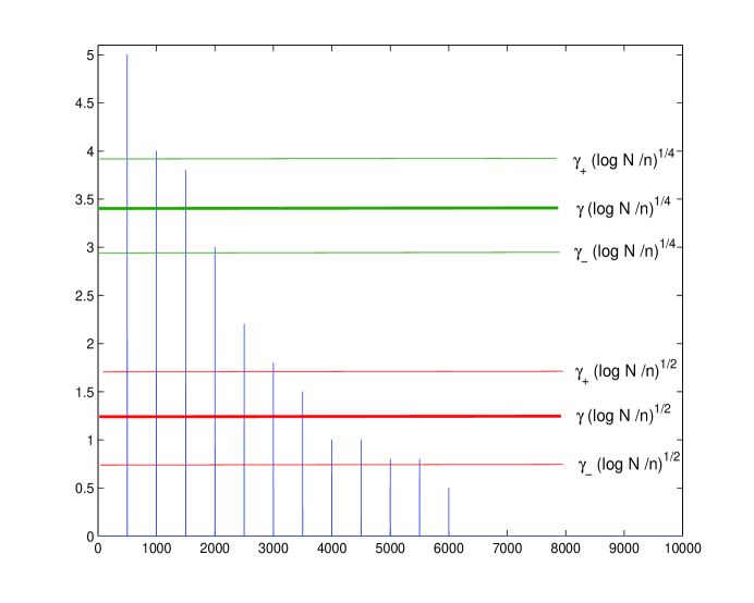
Figure 1: Schematic diagram of the D.T. and ASPCA thresholding schemes under the single component setting. The vertical lines depict the absolute values of the coordinates of the first eigenvector. The threshold for the D.T. scheme is $\gamma(\log N/n)^{1/4}$ while the thresholds for the ASPCA scheme is $\gamma(\log N/n)^{1/2}$. The schemes select the coordinates above the upper limits (indicated by the multiplier $\gamma_{+}$) and discard the coordinates below the lower limits (indicated by multiplier $\gamma_{-}$) with high probability. Here, $\gamma_{+}>\gamma>\gamma_{-}>0$ are generic constants.

5.1 ASPCA scheme

Based on the ideas described above, we now present the ASPCA algorithm. It first makes two stages of coordinate selection, whereas the final stage consists of an eigen-analysis of the submatrix of $\mathbf{S}$ corresponding to the selected coordinates. The algorithm is described below.

For any $\gamma>0$ define

$$I(\gamma)=\{k:\mathbf{S}_{kk}>1+\gamma\}.$$ (17)

Let $\gamma_{i}>0$ for $i=1,2$ and $\kappa>0$ be constants to be specified later.

• Let $I=I(\gamma_{1,n})$ where $\gamma_{1,n}=\gamma_{1}\sqrt{\log N/n}$.

• Denote the eigenvalues and eigenvectors of $\mathbf{S}_{II}$ by $\widehat{\ell}_{1}>\ldots>\widehat{\ell}_{m_{1}}$ and $\mathbf{f}_{1},\ldots,\mathbf{f}_{m_{1}}$ respectively, where $m_{1}=\min\{n,|I|\}$,

• Estimate $M$ by $\widehat{M}$ defined in Section 5.2.

• Let $\mathbf{E}=[\widehat{\ell}_{1}^{-1/2}\mathbf{f}_{1}\cdots\widehat{\ell}_{\widehat{M}}^{-1/2}\mathbf{f}_{\widehat{M}}]$ and $\mathbf{Q}=\mathbf{S}_{I^{c}I}\mathbf{E}.$

• Let $J=\{k\not\in I~{}:~{}(\mathbf{Q}\mathbf{Q}^{T})_{kk}>\gamma_{2,n}^{2}\}$ for some $\gamma_{2,n}>0$. Define $K=I\cup J$.

• For $\nu=1,\ldots,\widehat{M}$, denote by $\widehat{\theta}_{\nu}$ the $\nu$-th eigenvector of $\mathbf{S}_{KK}$, augmented with zeros in the coordinates $K^{c}$.

Remark 3

The ASPCA scheme is specified up to the choice of parameters $\gamma_{1},\gamma_{2,n}$ and $\kappa$, that determine its rate of convergence. It can be shown that choosing $\gamma_{1}=4$, $\kappa=\sqrt{2+\epsilon}$ for some $\epsilon>0$, and $\gamma_{2,n}$ given by

$$\gamma_{2,n}=\gamma_{2}\left(\sqrt{\frac{\log N}{n}}+\frac{1}{\kappa}\sqrt{\frac{\widehat{M}}{n}}\right)$$ (18)

with $\gamma_{2}=\kappa\sqrt{3/2}$ results in an asymptotically optimal rate. Again, we note that for finite $N$, $n$, the actual performance in terms of the risk of the resulting eigenvector estimate may have a strong dependence on the threshold. In practice, a delicate choice of thresholds can be highly beneficial. This issue, as well as the analysis of the risk of the ASPCA estimator, are beyond the scope of this paper and will be studied in a separate publication.

5.2 Estimation of $M$

Estimation of the dimension of the signal subspace is a classical problem. If the signal eigenvalues are strong enough (i.e., $\lambda_{\nu}>c\sqrt{N/n}$ for all $\nu=1,\ldots,M$, for some $c>1$ independent of $N,n$), then nonparametric methods that do not assume eigenvector sparsity can asymptotically estimate the correct $M$ (see, e.g. Kritchman and Nadler [2008]). When the eigenvectors are sparse, we can detect much weaker signals, as we describe below.

We estimate $M$ by thresholding the eigenvalues of the submatrix $\mathbf{S}_{\bar{I}\bar{I}}$ where $\bar{I}:=I(\bar{\gamma}\sqrt{\log N/n})$ for some $\bar{\gamma}>0$. Let $\bar{m}=\min\{n,|\bar{I}|\}$ and $\bar{\ell}_{1}>\ldots>\bar{\ell}_{\bar{m}}$ be the nonzero eigenvalues of $\mathbf{S}_{\bar{I}\bar{I}}$. Let $\alpha_{n}>0$ be a user-defined threshold. Then, define $\widehat{M}$ by

$$\widehat{M}:=\max\{1\leq k\leq\bar{m}:\bar{\ell}_{k}>1+\alpha_{n}\}.$$ (19)

It can be shown that under appropriate sparsity conditions, with a suitable choice of threshold $\alpha_{n}$, $\widehat{M}$ is a consistent estimator of $M$.

6 Summary and Discussion

In this paper we derived lower bounds on eigenvector estimates under three different sparsity regimes, denoted dense, sparse, and ultra-sparse. In the dense setting, Theorems 1 and 2 show that when $N/n\to 0$, the standard PCA estimator attains the optimal rate of convergence. In the ultra-sparse setting, Theorem 3.1 of Ma [2011] shows that the maximal risk of the ITSPCA estimator proposed by him attains the same asymptotic rate as the corresponding lower bound of Theorem 3. This implies that in the ultra-sparse setting, the lower bound on the minimax rate is indeed sharp. In a separate paper, we prove that in the ultra-sparse regime, the ASPCA algorithm also attains the minimax rate.

Finally, our analysis leaves some open questions in the intermediate sparse regime. According to Theorem 2, the lower bound in this regime is smaller by a factor of $(\log N)^{1-q/2}$, as compared to the ultra-sparse setting. Therefore, whether there exists an estimator (and in particular, one with low complexity), that attains the current lower bound, or whether this lower bound can be improved is an open question for future research.

Appendix A Proofs

A.1 Asymptotic risk of the standard PCA estimator

To prove Theorem 1, on the risk of the PCA estimator, we use the following lemmas.

Deviation of extreme eigenvalues of Wishart matrices

In our analysis, we shall need a probabilistic bound for deviations of $\parallel\frac{1}{n}\mathbf{Z}\mathbf{Z}^{T}-I\parallel$. This is given in the following lemma, proven in Section B.

Lemma A.1

Let $t_{n}=8(N_{n}/n)\sqrt{\log N_{n}/N_{n}}$ where $N_{n}=\max\{n,N\}$. Let $\mathbf{Z}$ be an $N\times n$ matrix with i.i.d. $N(0,1)$ entries. Then for any $c>0$, there exists $n_{c}\geq 1$ such that for all $n\geq n_{c}$,

$$\mathbb{P}\left(\parallel\frac{1}{n}\mathbf{Z}\mathbf{Z}^{T}-I_{N}\parallel>\frac{N}{n}+2\sqrt{\frac{N}{n}}+ct_{n}\right)\leq 2N_{n}^{-c^{2}}.$$ (A.1)

Deviation of quadratic forms

The following lemma is due to Johnstone [2001].

Lemma A.2

Let $\chi_{n}^{2}$ denote a Chi-square random variable with $n$ degrees of freedom. Then,

$$\mathbb{P}(\chi_{n}^{2}>n(1+\epsilon)) \leq e^{-3n\epsilon^{2}/16}\qquad(0<\epsilon<\frac{1}{2}),$$ (A.2)

$$\mathbb{P}(\chi_{n}^{2}<n(1-\epsilon)) \leq e^{-n\epsilon^{2}/4}~{}~{}~{}~{}~{}~{}~{}~{}(0<\epsilon<1),$$ (A.3)

$$\mathbb{P}(\chi_{n}^{2}>n(1+\epsilon)) \leq \frac{\sqrt{2}}{\epsilon\sqrt{n}}e^{-n\epsilon^{2}/4}~{}~{}(0<\epsilon<1/2,n\geq 16).$$ (A.4)

The following lemma is from Johnstone and Lu [2009].

Lemma A.3

Let $y_{1i},y_{2i},i=1,\ldots,n$ be two sequences of mutually independent, i.i.d. $N(0,1)$ random variables. Then for large $n$ and any $b$ s.t. $0<b\ll\sqrt{n}$,

$$\mathbb{P}\left(|\frac{1}{n}\sum_{i=1}^{n}y_{1i}y_{2i}|>\sqrt{b/n}\right)\leq 2\exp\left\{-\frac{3b}{2}+O(n^{-1}b^{2})\right\}.$$ (A.5)

Perturbation of eigen-structure

The following lemma from Paul [2005] is convenient for risk analysis of estimators of eigenvectors. Several variants of this lemma appear in the literature, most based on the approach of Kato [1980].

Lemma A.4

Let $A$ and $B$ be two symmetric $m\times m$ matrices. Let the eigenvalues of matrix $A$ be denoted by $\lambda_{1}(A)\geq\ldots\geq\lambda_{m}(A)$. Set $\lambda_{0}(A)=\infty$ and $\lambda_{m+1}(A)=-\infty$. For any $r\in\{1,\ldots,m\}$, if $\lambda_{r}(A)$ is a unique eigenvalue of $A$, i.e., if $\lambda_{r-1}(A)>\lambda_{r}(A)>\lambda_{r+1}(A)$, then denoting by $\mathbf{p}_{r}$ the eigenvector associated with the $r$-th eigenvalue,

$$\mathbf{p}_{r}(A+B)-\mbox{sign}(\mathbf{p}_{r}(A+B)^{T}\mathbf{p}_{r}(A))\mathbf{p}_{r}(A)=-H_{r}(A)B\mathbf{p}_{r}(A)+R_{r}$$ (A.6)

where $H_{r}(A):=\sum_{s\neq r}\frac{1}{\lambda_{s}(A)-\lambda_{r}(A)}P_{{\cal E}_{s}}(A)$ and $P_{{\cal E}_{s}}(A)$ denotes the projection matrix onto the eigenspace ${\cal E}_{s}$ corresponding to eigenvalue $\lambda_{s}(A)$ (possibly multi-dimensional). Define $\Delta_{r}$ and $\overline{\Delta}_{r}$ as

$$\Delta_{r} := \frac{1}{2}[\parallel H_{r}(A)B\parallel+|\lambda_{r}(A+B)-\lambda_{r}(A)|\parallel H_{r}(A)\parallel]$$ (A.7)

$$\overline{\Delta}_{r} = \frac{\parallel B\parallel}{\min_{1\leq j\neq r\leq m}|\lambda_{j}(A)-\lambda_{r}(A)|}~{}.$$ (A.8)

Then, the residual term $R_{r}$ can be bounded by

$$\hskip-14.45377pt\parallel R_{r}\parallel~{}\leq~{}\min\left\{10\overline{\Delta}_{r}^{2},\right.$$

$$\hskip-14.45377pt\left.\parallel H_{r}(A)B\mathbf{p}_{r}(A)\parallel\left[\frac{2\Delta_{r}(1+2\Delta_{r})}{1-2\Delta_{r}(1+2\Delta_{r})}+\frac{\parallel H_{r}(A)B\mathbf{p}_{r}(A)\parallel}{(1-2\Delta_{r}(1+2\Delta_{r}))^{2}}\right]\right\}$$ (A.9)

where the second bound holds only if $\Delta_{r}<(\sqrt{5}-1)/4$.

Remark A.1

We can simplify the bound on the perturbation in (A.4) to show that if $\overline{\Delta}_{r}\leq 1/4$, then

$$\parallel R_{r}\parallel\leq C\parallel H_{r}(A)B\mathbf{p}_{r}(A)\parallel\overline{\Delta}_{r}$$ (A.10)

where we can take $C=30$. To see this, note that $|\lambda_{r}(A+B)-\lambda_{r}(A)|\leq\parallel B\parallel$ and that $\parallel H_{r}(A)\parallel\leq[\min_{j\neq r}|\lambda_{j}(A)-\lambda_{r}(A)|]^{-1}$, so that,

$$\Delta_{r}\leq\parallel H_{r}(A)\parallel\parallel B\parallel\leq\overline{\Delta}_{r}.$$

Now, defining $\delta:=2\overline{\Delta}_{r}(1+2\overline{\Delta}_{r})$ and $\beta:=\parallel H_{r}(A)B\mathbf{p}_{r}(A)\parallel$, we have $10\overline{\Delta}_{r}^{2}\leq(5/2)\delta^{2}$, and the bound (A.4) may be expressed as

$$\parallel R_{r}\parallel\leq\frac{\beta\delta}{1-\delta}\min\left\{\frac{5}{2}\frac{\delta(1-\delta)}{\beta},1+\frac{\beta}{\delta(1-\delta)}\right\}~{}.$$

For $x>0$, the function $x\mapsto\min\{5x/2,1+1/x\}\leq 5/2$. Further, if $\overline{\Delta}_{r}<1/4$, then $\delta<3\overline{\Delta}_{r}<3/4$ and so we conclude that

$$\parallel R_{r}\parallel\leq 10\beta\delta\leq 30\beta\overline{\Delta}_{r}.$$

For notational simplicity, throughout this subsection, we write $\widehat{\theta}_{\nu}$ to mean $\widehat{\theta}_{\nu,PCA}$. Recall that the loss function $L(\widehat{\theta}_{\nu},\theta_{\nu})=\parallel\widehat{\theta}_{\nu}-\mbox{sign}\langle\widehat{\theta}_{\nu},\theta_{\nu}\rangle\theta_{\nu}\parallel^{2}$. Invoking Lemma A.4 with $A=\Sigma$ and $B=\mathbf{S}-\Sigma$ we get

$$\widehat{\theta}_{\nu}-\mbox{sign}\langle\widehat{\theta}_{\nu},\theta_{\nu}\rangle\theta_{\nu}=-H_{\nu}\mathbf{S}\theta_{\nu}+R_{\nu},$$ (A.11)

where

$$H_{\nu}\equiv H_{\nu}(\Sigma):=\sum_{1\leq\mu\neq\nu\leq M}\frac{1}{\lambda_{\mu}-\lambda_{\nu}}\theta_{\mu}\theta_{\mu}^{T}-\frac{1}{\lambda_{\mu}}P_{\perp},$$ (A.12)

where $P_{\perp}=I-\sum_{\mu=1}^{M}\theta_{\mu}\theta_{\mu}^{T}$. Note that $H_{\nu}\theta_{\nu}=0$ and that $H_{\nu}\Sigma\theta_{\nu}=0$. The key quantity in bounding the error term $R_{\nu}$ is

$$\overline{\Delta}_{\nu}=\max\{(\lambda_{\nu}-\lambda_{\nu+1})^{-1},(\lambda_{\nu-1}-\lambda_{\nu})^{-1}\}\parallel\mathbf{S}-\Sigma\parallel.$$

Indeed, from (A.10), when $\overline{\Delta}_{\nu}<1/4$, we have, for some constant $C>0$,

$$\parallel R_{\nu}\parallel\leq C\parallel H_{\nu}\mathbf{S}\theta_{\nu}\parallel\overline{\Delta}_{\nu}.$$

Set $\delta_{n\nu}^{\prime}=C\overline{\Delta}_{\nu}$. We will show that as $n\to\infty$, $\delta_{n\nu}^{\prime}\to 0$ with probability approaching 1 and

$$\parallel H_{\nu}\mathbf{S}\theta_{\nu}\parallel^{2}(1-\delta_{n\nu}^{\prime})^{2}\leq L(\widehat{\theta}_{\nu},\theta_{\nu})\leq\parallel H_{\nu}\mathbf{S}\theta_{\nu}\parallel^{2}(1+\delta_{n\nu}^{\prime})^{2}.$$ (A.13)

Theorem 1 then follows from an (exact, non-asymptotic) evaluation

$$\mathbb{E}\parallel H_{\nu}\mathbf{S}\theta_{\nu}\parallel^{2}=\frac{N-M}{nh(\lambda_{\nu})}+\frac{1}{n}\sum_{\mu\neq\nu}\frac{(1+\lambda_{\mu})(1+\lambda_{\nu})}{(\lambda_{\mu}-\lambda_{\nu})^{2}}~{}.$$ (A.14)

We begin with the evaluation of (A.14). First we derive a convenient representation of $H_{\nu}\mathbf{S}\theta_{\nu}$. In matrix form, model (2) becomes

$$\mathbf{X}=\sum_{\mu=1}^{M}\sqrt{\lambda_{\mu}}\theta_{\mu}v_{\mu}^{T}+\mathbf{Z}.$$ (A.15)

For $\nu=1,\ldots,M$, define

$$z_{\nu}=\mathbf{Z}^{T}\theta_{\nu},\qquad w_{\nu}=\mathbf{X}^{T}\theta_{\nu}=\sqrt{\lambda_{\nu}}v_{\nu}+z_{\nu}.$$ (A.16)

Define

$$\langle\mathbf{a},\mathbf{b}\rangle_{n}:=\frac{1}{n}\sum_{i=1}^{n}a_{i}b_{i}~{}~{}\mbox{for arbitrary}~{}~{}\mathbf{a},\mathbf{b}\in\mathbb{R}^{n}.$$ (A.17)

Then we have

$$\mathbf{S}\theta_{\nu}=\frac{1}{n}\mathbf{X}w_{\nu}=\sum_{\mu=1}^{M}\sqrt{\lambda_{\mu}}\langle v_{\mu},w_{\nu}\rangle_{n}\theta_{\mu}+\frac{1}{n}\mathbf{Z}w_{\nu}.$$

Using (A.16),

$$H_{\nu}\mathbf{Z}w_{\nu}=\sum_{\mu\neq\nu}\frac{\langle z_{\mu},w_{\nu}\rangle}{\lambda_{\mu}-\lambda_{\nu}}\theta_{\mu}-\frac{1}{\lambda_{\nu}}P_{\perp}\mathbf{Z}w_{\nu}.$$

Using (A.12), $H_{\nu}\theta_{\mu}=(\lambda_{\mu}-\lambda_{\nu})^{-1}\theta_{\mu}$ for $\mu\neq\nu$, and we arrive at the desired representation

$$H_{\nu}\mathbf{S}\theta_{\nu}=\sum_{\mu\neq\nu}\frac{\langle w_{\mu},w_{\nu}\rangle_{n}}{\lambda_{\mu}-\lambda_{\nu}}\theta_{\mu}-\frac{1}{n\lambda_{\nu}}P_{\perp}\mathbf{Z}w_{\nu}.$$ (A.18)

By orthogonality,

$$\parallel H_{\nu}\mathbf{S}\theta_{\nu}\parallel^{2}=\sum_{\mu\neq\nu}\frac{\langle w_{\mu},w_{\nu}\rangle_{n}^{2}}{(\lambda_{\mu}-\lambda_{\nu})^{2}}+\frac{1}{n^{2}\lambda_{\nu}^{2}}w_{\nu}^{T}\mathbf{Z}^{T}P_{\perp}\mathbf{Z}w_{\nu}.$$ (A.19)

Now we compute the expectation. One verifies that $z_{\nu}\sim N(0,I_{n})$ independently of each other and of each $v_{\nu}\sim N(0,I_{n})$, so that $w_{\nu}\sim N(0,(1+\lambda_{\nu})I_{n})$ independently. Hence, for $\mu\neq\nu$,

$$\mathbb{E}\langle w_{\mu},w_{\nu}\rangle_{n}^{2} = n^{-2}\mathbb{E}\mbox{tr}(w_{\nu}w_{\nu}^{T}w_{\mu}w_{\mu}^{T})$$ (A.20)

$$= n^{-2}\mbox{tr}((1+\lambda_{\mu})(1+\lambda_{\nu})I_{n})$$

$$= n^{-1}(1+\lambda_{\mu})(1+\lambda_{\nu}).$$

From (A.16),

$$\mathbb{E}[w_{\nu}^{T}\mathbf{Z}^{T}P_{\perp}\mathbf{Z}w_{\nu}|\mathbf{Z}] = z_{\nu}^{T}\mathbf{Z}^{T}P_{\perp}\mathbf{Z}z_{\nu}+\lambda_{\nu}\mathbb{E}[v_{\nu}^{T}\mathbf{Z}^{T}P_{\perp}\mathbf{Z}v_{\nu}|\mathbf{Z}]$$

$$= \mbox{tr}(\mathbf{Z}\mathbf{Z}^{T}P_{\perp}\mathbf{Z}\mathbf{Z}^{T}\theta_{\mu}\theta_{\mu}^{T})+\lambda_{\nu}\mbox{tr}(P_{\perp}\mathbf{Z}\mathbf{Z}^{T}).$$

Now, it can be easily verified that if $W:=\mathbf{Z}\mathbf{Z}^{T}\sim$ $W_{N}(n,I)$, then for arbitrary symmetric $N\times N$ matrices $Q$, $R$, we have,

$$\mathbb{E}\mbox{tr}(WQWR)=n[\mbox{tr}(QR)+\mbox{tr}(Q)\mbox{tr}(R)]+n^{2}\mbox{tr}(QR).$$ (A.21)

Taking $Q=P_{\perp}$ and $R=\theta_{\mu}\theta_{\mu}^{T}$, by (A.21) we have

$$\mathbb{E}[w_{\nu}^{T}\mathbf{Z}P_{\perp}\mathbf{Z}w_{\nu}]=n\mbox{tr}(P_{\perp})+n\lambda_{\nu}\mbox{tr}(P_{\perp})=n(N-M)(1+\lambda_{\nu}).$$ (A.22)

Combining (A.20) with (A.22) in computing the expectation of (A.19), we obtain the expression (A.14) for $\mathbb{E}\parallel H_{\nu}\mathbf{S}\theta_{\nu}\parallel^{2}$.

Bound for $\parallel\mathbf{S}-\Sigma\parallel$

We begin with the decomposition of the sample covariance matrix $\mathbf{S}$. Introduce the abbreviation $\xi_{\mu}=n^{-1}\mathbf{Z}v_{\mu}$. Then,

$$\mathbf{S}=\sum_{\mu=1}^{M}\sum_{\mu^{\prime}=1}^{M}\sqrt{\lambda_{\mu}\lambda_{\mu^{\prime}}}\langle v_{\mu},v_{\mu^{\prime}}\rangle_{n}\theta_{\mu}\theta_{\mu^{\prime}}^{T}+\sum_{\mu=1}^{M}\sqrt{\lambda_{\mu}}(\theta_{\mu}\xi_{\mu}^{T}+\xi_{\mu}\theta_{\mu}^{T})+n^{-1}\mathbf{Z}\mathbf{Z}^{T}$$ (A.23)

and hence

$$\parallel\mathbf{S}-\Sigma\parallel \leq \sum_{\mu=1}^{M}\sum_{\mu^{\prime}=1}^{M}\sqrt{\lambda_{\mu}\lambda_{\mu^{\prime}}}|\langle v_{\mu},v_{\mu^{\prime}}\rangle_{n}-\delta_{\mu\mu^{\prime}}|$$ (A.24)

$$+2\sum_{\mu=1}^{M}\sqrt{\lambda_{\mu}}\parallel\xi_{\mu}\parallel+\parallel n^{-1}\mathbf{Z}\mathbf{Z}^{T}-I\parallel,$$

where $\delta_{\mu\mu^{\prime}}$ denotes the Kronecker symbol. Let $D_{1}$ be the intersection of all the events (for some constant $c>0$):

$$D_{11} := \{|\parallel v_{\mu}\parallel_{n}^{2}-1|\leq 2c\sqrt{n^{-1}\log n},~{}1\leq\mu\leq M\},$$

$$D_{12} := \{|\langle v_{\mu},v_{\nu}\rangle_{n}|\leq c\sqrt{n^{-1}\log n},~{}1\leq\mu\neq\mu^{\prime}\leq M\},$$

$$D_{13} := \{\parallel\xi_{\mu}\parallel\leq(1+2c\sqrt{N^{-1}\log n})\sqrt{\frac{N}{n}},~{}1\leq\mu\leq M\}.$$

Since $v_{\nu}\stackrel{{\scriptstyle i.i.d.}}{{\sim}}N(0,I_{n})$ independent of $\mathbf{Z}$, we have $\mathbf{Z}v_{\nu}/\parallel v_{\nu}\parallel\sim N(0,I_{N})$ independently of $v_{\nu}$, and $\parallel v_{\nu}\parallel^{2}\sim\chi_{n}^{2}$. Moreover,

$$D_{11}\cap\{\parallel\mathbf{Z}v_{\mu}\parallel^{2}/\parallel v_{\mu}\parallel^{2}\leq 1+2c\sqrt{N^{-1}\log n},~{}1\leq\mu\leq M\}\subset D_{13}.$$

Hence, we use Lemmas A.2 and A.3 to prove that

$$1-\mathbb{P}(D_{1})\leq 3Mn^{-c^{2}}+M(M-1)n^{-(3/2)c^{2}+O(n^{-1}\log n)}.$$ (A.25)

Define $D_{2}$ to be be the event that

$$D_{2}:=\left\{\parallel\frac{1}{n}\mathbf{Z}\mathbf{Z}^{T}-I_{N}\parallel\leq\frac{N}{n}+2\sqrt{\frac{N}{n}}+ct_{n}\right\},$$ (A.26)

with $t_{n}$ as in Lemma A.1 with $N_{n}=\max\{n,N\}=n$ so that $t_{n}=8\sqrt{n^{-1}\log n}$. Lemma A.1 also establishes that $1-\mathbb{P}(D_{2})\leq 2n^{-c^{2}}$. Using the notation $\eta_{n}:=(N^{-1}\log n)^{1/2}$, we have, on $D_{1}\cap D_{2}$,

$$\parallel\mathbf{S}-\Sigma\parallel \leq 2c(\sum_{\mu=1}^{M}\sqrt{\lambda_{\mu}})^{2}\eta_{n}+2(\sum_{\mu=1}^{M}\lambda_{\mu})(1+2c\eta_{n})\sqrt{\frac{N}{n}}$$ (A.27)

$$+2\sqrt{\frac{N}{n}}+\frac{N}{n}+ct_{n}.$$

Recalling that $\rho_{\nu}=\lambda_{\nu}/\lambda_{1}$ for $\nu=1,\ldots,M$, we have for large $n$ that

$$\overline{\Delta}_{\nu}\leq C_{\nu}(\rho)\frac{\parallel\mathbf{S}-\Sigma\parallel}{\lambda_{1}},$$

where, say $C_{\nu}(\rho)=2\max\{(\rho_{\nu}-\rho_{\nu+1})^{-1},(\rho_{\nu-1}-\rho_{\nu})^{-1}\}$. Observe that $t_{n}/\lambda_{1}=8\eta_{n}\sqrt{N/(n\lambda_{1})^{2}}$. Now, substitute (A.27) to conclude that there are functions $B_{i}(\rho)$ such that on $D_{n}:=D_{1}\cap D_{2}$,

$$\overline{\Delta}_{\nu}\leq B_{1}(\rho)\eta_{n}+B_{2}(\rho)(1+2c\eta_{n})\sqrt{\frac{N}{n\lambda_{1}}}+2\sqrt{\frac{N}{n\lambda_{1}^{2}}}+\frac{N}{n\lambda_{1}}+8c\eta_{n}\sqrt{\frac{N}{n\lambda_{1}^{2}}}~{}.$$

Our assumptions imply that

$$\eta_{n}=\sqrt{\frac{\log n}{N}}\to 0\qquad\mbox{and}\qquad\frac{N}{n\lambda_{1}^{2}}+\frac{N}{n\lambda_{1}}=\frac{N}{nh(\lambda_{1})}\to 0,$$

so that $\overline{\Delta}_{\nu}\to 0$. To summarize, choose $c=\sqrt{2}$, say, so that on $D_{n}$, which has probability at least $1-O(n^{-2})$, we have $\delta_{n\nu}^{\prime}\to 0$. This completes the proof of (A.13).

Theorem 1 now follows from noticing that $L(\widehat{\theta}_{\nu},\theta_{\nu})\leq 2$ and so

$$\mathbb{E}[L(\widehat{\theta}_{\nu},\theta_{\nu}),(D_{1}\cap D_{2})^{c}]\leq 2\mathbb{P}((D_{1}\cap D_{2})^{c})=O(N_{n}^{-2})=o(\mathbb{E}\parallel H_{\nu}\mathbf{S}\theta_{\nu}\parallel^{2}),$$

and an additional computation using (A.19) which shows that

$$\mathbb{E}[\parallel H_{\nu}\mathbf{S}\theta_{\nu}\parallel^{2},D_{n}^{c}]\leq(\mathbb{E}[\parallel H_{\nu}\mathbf{S}\theta_{\nu}\parallel^{4})^{1/2}P(D_{n}^{c})=o(\mathbb{E}[\parallel H_{\nu}\mathbf{S}\theta_{\nu}\parallel^{2}).$$

A.2 Lower bound on the minimax risk

In this subsection, we prove Theorems 2 and 3. The key idea in the proofs is to utilize the geometry of the parameter space in order to construct appropriate finite dimensional subproblems for which bounds are easier to obtain. We first give an overview of the general machinery used in the proof.

Risk bounding strategy

A key tool for deriving lower bounds on the minimax risk is Fano’s Lemma. In this subsection, we use superscripts on vectors $\theta$ as indices, not exponents. First, we construct a large finite subset ${\cal F}$ of $\Theta_{q}^{M}(C_{1},\ldots,C_{M})$, such that the following property holds, for a given $\nu\in\{1,\ldots,M\}$.

• If $\boldsymbol{\theta}^{1},\boldsymbol{\theta}^{2}\in{\cal F}$, then $L(\theta_{\nu}^{1},\theta_{\nu}^{2})\geq 4\delta$, for some $\delta>0$ (to be chosen).

This property will be referred to as “$4\delta$-distinguishability in $\theta_{\nu}$”. Given any estimator $\widehat{\boldsymbol{\theta}}$ of $\boldsymbol{\theta}$, based on data $\mathbf{X}_{n}=(X_{1},\ldots,X_{n})$, define a new estimator $\phi(\mathbf{X}_{n})=\boldsymbol{\theta}^{*}$, whose $M$ components are given by $\theta^{*}_{\nu}=\arg\min_{\boldsymbol{\theta}\in{\cal F}}L(\widehat{\theta}_{\nu},\theta_{\nu})$, where $\widehat{\theta}_{\nu}$ is the $\nu$-th column of $\widehat{\boldsymbol{\theta}}$. Then, by Chebyshev’s inequality and the $4\delta$-distinguishability in $\theta_{\nu}$, it follows that

$$\sup_{\boldsymbol{\theta}\in\Theta_{q}^{M}(C_{1},\ldots,C_{M})}\mathbb{E}_{\boldsymbol{\theta}}L(\widehat{\theta}_{\nu},\theta_{\nu}) \geq \delta\sup_{\boldsymbol{\theta}\in{\cal F}}\mathbb{P}_{\boldsymbol{\theta}}(\phi(\mathbf{X}_{n})\neq\boldsymbol{\theta}).$$ (A.28)

The task is then to find an appropriate lower bound for the quantity on the right hand side of (A.28). For this, we use the following version of Fano’s lemma, due to Birgé [2001], modifying a result of Yang and Barron [1999] (p. 1570-71).

Lemma A.5

Let $\{P_{\theta}:\theta\in\Theta\}$ be a family of probability distributions on a common measurable space, where $\Theta$ is an arbitrary parameter set. Let $p_{max}$ be the minimax risk over $\Theta,$ with the loss function $L^{\prime}(\theta,\theta^{\prime})=\mathbf{1}_{\theta\neq\theta^{\prime}}$,

$$p_{max}=\inf_{T}\sup_{\theta\in\Theta}\mathbb{P}_{\theta}(T\neq\theta)=\inf_{T}\sup_{\theta\in\Theta}\mathbb{E}L^{\prime}(\theta,T),$$

where $T$ denotes an arbitrary estimator of $\theta$ with values in $\Theta$. Then for any finite subset ${\cal F}$ of $\Theta$, with elements $\theta_{1},\ldots,\theta_{J}$ where $J=|{\cal F}|$,

$$p_{max}\geq 1-\inf_{Q}~{}\frac{J^{-1}\sum_{i=1}^{J}K(P_{i},Q)+\log 2}{\log J}$$ (A.29)

where $P_{i}=\mathbb{P}_{\theta_{i}}$, and $Q$ is an arbitrary probability distribution, and $K(P_{i},Q)$ is the Kullback-Leibler divergence of $Q$ from $P_{i}$.

The following lemma, proven in Section B, gives the Kullback-Leibler discrepancy corresponding to two different values of the parameter.

Lemma A.6

Let $\boldsymbol{\theta}^{j}:=[\theta_{1}^{j}:\ldots:\theta_{M}^{j}]$, $j=1,2$ be two parameters (i.e., for each $j$, $\theta_{k}^{j}$’s are orthonormal). Let $\Sigma_{j}$ denote the matrix given by (1) with $\boldsymbol{\theta}=\boldsymbol{\theta}^{j}$ (and $\sigma=1$). Let $P_{j}$ denote the joint probability distribution of $n$ i.i.d. observations from $N(0,\Sigma_{j})$. Then the Kullback-Leibler discrepancy of $P_{2}$ with respect to $P_{1}$ is given by

$${\cal K}_{1,2}:=K(\boldsymbol{\theta}^{1},\boldsymbol{\theta}^{2})=\frac{n}{2}\Bigg{[}\sum_{\nu=1}^{M}\eta(\lambda_{\nu})\lambda_{\nu}-\sum_{\nu=1}^{M}\sum_{\mu=1}^{M}\eta(\lambda_{\nu})\lambda_{\mu}|\langle\theta_{\mu}^{1},\theta_{\nu}^{2}\rangle|^{2}\Bigg{]},$$ (A.30)

where $\eta(\lambda)=\lambda/(1+\lambda)$.

Geometry of the hypothesis set and Sphere Packing

Next, we describe the construction of a large set of hypotheses ${\cal F}$, satisfying the $4\delta$ distinguishability condition. Our construction is based on the well studied sphere packing problem, namely how many unit vectors can be packed onto $\mathbb{S}^{m-1}$, with given minimal pairwise distance between any two vectors.

Here we follow the construction due to Zong [1999] (p. 77). Let $m$ be a large positive integer, and $m_{0}=\lfloor 2m/9\rfloor$. Define $Y_{m}^{*}$ as the maximal set of points of the form ${\bf z}=(z_{1},\ldots,z_{m})$ in $\mathbb{S}^{m-1}$ such that the following is true:

$$\sqrt{m_{0}}z_{i}\in\{-1,0,1\}~{}\forall~{}i,~{}~{}\sum_{i=1}^{m}|z_{i}|=\sqrt{m_{0}}~{}~{}\mbox{and, for}~{}~{}{\bf z},{\bf z}^{\prime}\in Y_{m}^{*},~{}~{}\parallel{\bf z}-{\bf z}^{\prime}\parallel\geq 1.$$

For any $m\geq 1$, the maximal number of points lying on $\mathbb{S}^{m-1}$ such that any two points are at distance at least 1, is called the kissing number of an $m$-sphere. Zong [1999] uses the construction described above to derive a lower bound on the kissing number, by showing that $|Y_{m}^{*}|\geq(9/8)^{m(1+o(1))}$ for $m$ large.

Next, for $m<N-M$ we use the sets $Y_{m}^{*}$ to construct our hypothesis set $\cal F$ of same size, $|{\cal F}|=|Y_{m}^{*}|$. To this end, let $\{{\bf e}_{\mu}\}_{\mu=1}^{N}$ denote the standard basis of $\mathbb{R}^{N}$. Our initial set ${\boldsymbol{\theta}}^{0}$ is composed of the first $M$ standard basis vectors, ${\boldsymbol{\theta}}^{0}=[{\bf e}_{1}:\ldots:{\bf e}_{M}]$. Then, for fixed $\nu$, and values of $m,r$ yet to be determined, each of the other hypotheses ${\boldsymbol{\theta}}^{j}\in{\cal F}$ has the same vectors as ${\bf\theta}^{0}$ for $k\neq\nu$. The difference is that the $\nu$-th vector is instead given by

$$\theta_{\nu}^{j}=\sqrt{1-r^{2}}~{}\mathbf{e}_{\nu}+r\sum_{l=1}^{m}z_{l}^{j}\mathbf{e}_{M+l},~{}~{}~{}j=1,\ldots,|{\cal F}|,$$ (A.31)

where $\mathbf{z}^{j}=(z_{1}^{j},\ldots,z_{m}^{j})$, $j\geq 1$, is an enumeration of the elements of $Y_{m}^{*}$. Thus $\theta_{\nu}^{j}$ perturbs $\mathbf{e}_{\nu}$ in subsets of the fixed set of coordinates $\{M+1,\dots,M+m\}$, according to the sphere packing construction for $\mathbb{S}^{m-1}$.

The construction ensures that $\theta_{1}^{j},\ldots,\theta_{M}^{j}$ are orthonormal for each $j$. Furthermore, (A.30) simplifies to

$$K(\boldsymbol{\theta}^{j},\boldsymbol{\theta}^{0})=\frac{1}{2}nh(\lambda_{\nu})(1-(\langle\theta_{\nu}^{j},\theta_{\nu}^{0}\rangle)^{2})=\frac{1}{2}nh(\lambda_{\nu})r^{2},~{}~{}j=1,\ldots,|{\cal F}|.$$ (A.32)

Finally, by construction, for any $\boldsymbol{\theta}^{j},\boldsymbol{\theta}^{k}\in{\cal F}$ with $j\neq k$

$$L(\theta_{\nu}^{j},\theta_{\nu}^{k})\geq r^{2},$$ (A.33)

In other words, the set ${\cal F}$ is $r^{2}$-distinguishable in $\theta_{\nu}$. Consequently, combining (A.28) and (A.32),

$$R_{\nu}^{*}=\inf_{\hat{\theta}_{\nu}}\sup_{\Theta_{q}(\mathbf{C})}\mathbb{E}L(\hat{\theta}_{\nu},\theta_{\nu})\geq(r^{2}/4)[1-a(r,\mathcal{F})],$$ (A.34)

with

$$a(r,\mathcal{F})=\frac{\tfrac{1}{2}nh(\lambda_{\nu})r^{2}+\log 2}{\log|\mathcal{F}|}~{}.$$ (A.35)

Proof of Theorem 2

Let $m$ be an integer yet to be specified and let $r\in(0,1)$. Let $Y_{m}^{*}$ be the sphere-packing set defined above, and let $\cal F$ be the corresponding set of hypotheses, defined via (A.31).

Let $c_{1}=\log(9/8)$, then we have $\log|\mathcal{F}|\geq b_{m}c_{1}m$, where $b_{m}\to 1$ as $m\to\infty$. Inserting the following value for $r=r(m)$,

$$r^{2}=\frac{c_{1}m}{nh(\lambda_{\nu})},$$ (A.36)

into Eq. (A.35) gives that

$$a(r,\mathcal{F})\leq\frac{\tfrac{1}{2}c_{1}m+\log 2}{b_{m}c_{1}m}~{}.$$

Therefore, so long as $m\geq m_{*}$, an absolute constant, we have $a(r,\mathcal{F}_{0})\leq 3/4$.

We need to ensure that $\theta_{\nu}^{j}\in\Theta_{q}(C_{\nu})$. Since exactly $m_{0}$ coordinates are non-zero out of $\{M+1,\dots,M+m\}$,

$$\|\theta_{\nu}^{j}\|_{q}^{q}=(1-r^{2})^{q/2}+r^{q}m_{0}^{1-q/2}\leq 1+a_{q}r^{q}m^{1-q/2}$$

where $a_{q}=(2/9)^{1-q/2}$. A sufficient condition for $\theta_{\nu}^{(j)}\in\Theta_{q}(C_{\nu})$ is that

$$a_{q}m(r^{2}/m)^{q/2}\leq\bar{C}_{\nu}^{q}.$$ (A.37)

Substituting (A.36) puts this into the form

$$m\leq\frac{1}{a_{q}c_{1}^{q/2}}\bar{C}_{\nu}^{q}[nh(\lambda_{\nu})]^{q/2}.$$

To simultaneously ensure that (i) $r^{2}<1$, (ii) $m$ does not exceed the number of available co-ordinates, $N-M$, and (iii) $\theta_{\nu}^{j}\in\Theta_{q}(C_{\nu})$, we set

$$m=\min\{\lfloor nh(\lambda_{\nu})\rfloor,N-M,\lfloor A_{q}\bar{C}_{\nu}^{q}(nh(\lambda_{\nu}))^{q/2}\rfloor\},$$

where $A_{q}=1/(a_{q}c_{1}^{q/2})$. Recalling the notations (9), (10) and (11), this becomes (without loss of generality assuming $nh(\lambda_{\nu})$ and $m_{\nu}$ to be integers)

$$m=\min\{\tau_{\nu}^{-2},N^{\prime},m_{\nu}\}=\tau_{\nu}^{-2}\min\{1,\tau_{\nu}^{2}\cdot\min\{N^{\prime},m_{\nu}\}\}$$

and Theorem 2 follows.

Proof of Theorem 3

The construction of the set of hypotheses in the proof of Theorem 2 considered a fixed set of potential non-zero coordinates, namely $\{M+1,\ldots,M+m\}$. However, in the ultra-sparse setting, when the effective dimension is significantly smaller than the nominal dimension $N$, it is possible to construct a much larger collection of hypotheses by allowing the set of non-zero coordinates to span all remaining coordinates $\{M+1,\ldots,N\}$.

In the proof of Theorem 3 we shall use the following lemma, proven in Section B. Call $A\subset\{1,\ldots,N\}$ an $m-$set if $|A|=m$.

Lemma A.7

Let $k$ be fixed, and let $\mathcal{A}_{k}$ be the maximal collection of $m-$sets such that the intersection of any two members has cardinality at most $k-1$. Then, necessarily,

$$|\mathcal{A}_{k}|\geq\binom{N}{k}\bigg{/}\binom{m}{k}^{2}.$$ (A.38)

Let $k=[m_{0}/2]+1$ and $m_{0}=[\beta m]$ with $0<\beta<1.$ Suppose that $m,N\rightarrow\infty$ with $m=o(N)$. Then

$$|\mathcal{A}_{k}|\geq\exp[N\mathcal{E}(\beta m/2N)-2m\mathcal{E}(\beta/2)](1+o(1)).$$ (A.39)

where ${\cal E}(x)$ is the Shannon entropy function,

$${\cal E}(x)=-x\log(x)-(1-x)\log(1-x),~{}~{}0<x<1.$$

Let $\pi$ be an $m-$set contained in $\{M+1,\dots,N\}$, and construct a family $\mathcal{F}_{\pi}$ by modifying (A.31) to use the set $\pi$ rather than the fixed set $\{M+1,\dots,M+m\}$ as in Theorem 2:

$$\theta_{\nu}^{(j,\pi)}=\sqrt{1-r^{2}}~{}\mathbf{e}_{\nu}+r\sum_{l\in\pi}z_{l}^{j}\mathbf{e}_{l},~{}~{}~{}j=1,\ldots,|Y_{m}^{*}|.$$

We will choose $m$ below to ensure that $\theta_{\nu}^{(j,\pi)}\in\Theta_{q}(C_{\nu})$. Let ${\cal P}$ be a collection of sets $\pi$ such that, for any two sets $\pi$ and $\pi^{\prime}$ in ${\cal P}$, the set $\pi\cap\pi^{\prime}$ has cardinality at most $m_{0}/2$. This ensures that the sets ${\cal F}_{\pi}$ are disjoint for $\pi\neq\pi^{\prime}$, since each $\theta_{\nu}^{(j,\pi)}$ is nonzero in exactly $m_{0}+1$ coordinates. This construction also ensures that

$$\mbox{for all}~{}~{}\mathbf{y},\mathbf{y}^{\prime}\in\bigcup_{\pi\in\cal P}{\cal F}_{\pi},\quad L(\mathbf{y},\mathbf{y}^{\prime})\geq\left(\frac{m_{0}}{2}+\frac{m_{0}}{2}\right)\left(\frac{r}{\sqrt{m_{0}}}\right)^{2}=r^{2}.$$

Define ${\cal F}:=\bigcup_{\pi\in\cal P}{\cal F}_{\pi}$. Then

$$|{\cal F}|=|\bigcup_{\pi\in\cal P}{\cal F}_{\pi}|=|{\cal P}|~{}|Y_{m}^{*}|\geq|{\cal P}|(9/8)^{m(1+o(1))}.$$ (A.40)

By Lemma A.7, there is a collection ${\cal P}$ such that $|{\cal P}|$ is at least $\exp([N{\cal E}(m/9N)-2m{\cal E}(1/9)](1+o(1)))$. Since ${\cal E}(x)\geq-x\log x$, it follows from (A.40) that,

$$\frac{\log|{\cal F}|}{m}\geq\left(\frac{1}{9}\log\frac{9N}{m}-2{\cal E}(1/9)\right)+\log(9/8)(1+o(1))\geq\frac{\alpha}{9}\log N+O(1),$$

since $m=O(N^{1-\alpha})$.

Proceeding as for Theorem 2, we have $\log|\mathcal{F}|\geq b_{m}(\alpha/9)m\log N$, where $b_{m}\to 1$. Let us set (with $m$ still to be specified)

$$r^{2}=m\frac{(\alpha/9)\log N}{nh(\lambda_{\nu})}=m\bar{\tau}_{\nu}^{2},$$ (A.41)

Again, we need to ensure that $\theta_{\nu}^{(j,\pi)}\in\Theta_{q}(C_{\nu})$, which as before is implied by (A.37). Substituting (A.41) puts this into the form

$$m\leq\bar{m}_{\nu}=a_{q}^{-1}(\bar{C}_{\nu}/\bar{\tau}_{\nu})^{q}.$$

To simultaneously ensure that (i) $r^{2}<1$; (ii) $m$ does not exceed the number of available co-ordinates, $N-M$; and (iii) $\theta_{\nu}^{j}\in\Theta_{q}(C_{\nu})$, we set

$$m=\min\{\lfloor\bar{\tau}_{\nu}^{-2}\rfloor,N-M,\lfloor a_{q}^{-1}(\bar{C}_{\nu}^{q}/\bar{\tau}_{\nu})^{q}\rfloor\}.$$

As $n,N\to\infty$, we have that $m=\lfloor a_{q}^{-1}(\bar{C}_{\nu}/\bar{\tau}_{\nu})^{q}\rfloor$, and Theorem 3 follows.

A.3 Lower bound on the risk of the D.T. estimator

To prove Theorem 4, assume w.l.g. that $\langle\widehat{\theta}_{1,DT},\theta_{1}\rangle>0$, and decompose the loss as

$$L(\widehat{\theta}_{1,DT},\theta_{1})=\parallel\theta_{1}-\theta_{1,I}\parallel^{2}+\parallel\widehat{\theta}_{1,DT}-\theta_{1,I}\parallel^{2},$$ (A.42)

where $I=I(\gamma_{n})$ is the set of coordinates selected by the D.T. scheme and $\theta_{1,I}$ denotes the subvector of $\theta_{1}$ corresponding to this set. Note that, in (A.42), the first term on the right can be viewed as a bias term while the second term can be seen as a variance term.

We choose a particular vector $\theta_{1}=\theta_{*}\in\Theta_{q}(C)$ so that

$$\mathbb{E}\parallel\theta_{*}-\theta_{*,I}\parallel^{2}\geq K\bar{C}^{q}n^{-\frac{1}{2}(1-q/2)}.$$ (A.43)

This, together with (A.42), proves Theorem 4 since the worst case risk is clearly at least as large as (A.43). Accordingly, set $r_{n}=\bar{C}^{q/2}n^{-\frac{1}{4}(1-q/2)}$, where $\bar{C}^{q}=C^{q}-1$. Since $C^{q}n^{q/4}=o(n^{1/2})$, we have $r_{n}=o(1)$, and so for sufficiently large $n$, we can take $r_{n}<1$ and define

$$\theta_{*,k}=\begin{cases}\sqrt{1-r_{n}^{2}}&~{}\mbox{if}~{}~{}k=1\\ \frac{r_{n}}{\sqrt{m_{n}}}&~{}\mbox{if}~{}~{}2\leq k\leq m_{n}+1\\ 0&~{}\mbox{if}~{}~{}m_{n}+2\leq k\leq N\end{cases}$$

where $m_{n}=\lfloor(1/2)\bar{C}^{q}n^{q/4}\rfloor$. Then by construction $\theta_{*}\in\Theta_{q}(C)$, since

$$\sum_{k=1}^{N}|\theta_{*,k}|^{q}=(1-r_{n}^{2})^{q/2}+r_{n}^{q}m_{n}^{1-q/2}<1+r_{n}^{q}m_{n}^{1-q/2}\leq 1+\frac{\bar{C}^{q}}{2^{1-q/2}}<C^{q},$$

where the last inequality is due to $q\in(0,2)$ and $\bar{C}^{q}=C^{q}-1$.

For notational convenience, let $\alpha_{n}=\gamma\sqrt{\log N/n}$. Recall that D.T. selects all coordinates $k$ for which $\mathbf{S}_{kk}>1+\alpha_{n}$. Therefore, coordinate $k$ is not selected with probability

$$p_{k}=\mathbb{P}(\mathbf{S}_{kk}<1+\alpha_{n})=\mathbb{P}\left(\frac{W_{n}}{n}<\frac{1+\alpha_{n}}{1+\lambda_{1}\theta_{*,k}^{2}}\right)$$ (A.44)

where $W_{n}\sim\chi_{n}^{2}$. Notice that, for $k=2,\ldots,m_{n}+1$, $p_{k}=p_{2}$, and $\theta_{*,k}=0$ for $k>m_{n}+1$. Hence,

$$\mathbb{E}\parallel\theta_{*}-\theta_{*,I}\parallel^{2}=\sum_{k=1}^{N}p_{k}|\theta_{*,k}|^{2}>p_{2}\sum_{k=2}^{m_{n}+1}|\theta_{*,k}|^{2}=p_{2}r_{n}^{2}=p_{2}\bar{C}^{q}n^{-\frac{1}{2}(1-q/2)}.$$

Thus, to finish the proof of Theorem 4, it is enough to show that $p_{2}>1-A_{n}$ for some $A_{n}$ that converges to 0 as $n\to\infty$. Rewrite (A.44) as

$$p_{k}=\mathbb{P}\left(\frac{W_{n}}{n}<1+\epsilon_{k}\right)=1-\mathbb{P}\left(\frac{W_{n}}{n}\geq 1+\epsilon_{k}\right)~{}~{}\mbox{where}~{}~{}\epsilon_{k}=\frac{\alpha_{n}-\lambda_{1}|\theta_{*,k}|^{2}}{1+\lambda_{1}|\theta_{*,k}|^{2}}~{}.$$

Since $|\theta_{*,2}|^{2}=r_{n}^{2}/m_{n}=2n^{-1/2}(1+o(1))$, it follows that

$$\epsilon_{2}=\frac{\gamma\sqrt{\frac{\log N}{n}}-\lambda_{1}\frac{r_{n}^{2}}{m_{n}}}{1+\lambda_{1}\frac{r_{n}^{2}}{m_{n}}}=\frac{1}{\sqrt{n}}\left(\frac{\gamma\sqrt{\log N}-2\lambda_{1}}{1+2\lambda_{1}/\sqrt{n}}\right)(1+o(1))$$

so that $n\epsilon_{2}^{2}\to\infty$ as $n\to\infty$. This, together with (A.3), shows that $p_{2}\geq 1-A_{n}$ where we can choose $A_{n}=\exp(-3n\epsilon_{2}^{2}/16)=o(1)$.

Appendix B Proof of relevant lemmas

B.1 Proof of Lemma A.1

We use the following result on extreme eigenvalues of Wishart matrices by Davidson and Szarek [2001].

Lemma A.8

Let $Z$ be a $p\times q$ matrix of i.i.d. $N(0,1)$ entries with $p\leq q$. Let $s_{max}(Z)$ and $s_{min}(Z)$ denote the largest and the smallest singular value of $Z$, respectively. Then,

$$\mathbb{P}(s_{max}(\frac{1}{\sqrt{q}}Z)>1+\sqrt{p/q}+t) \leq e^{-qt^{2}/2},$$ (A.45)

$$\mathbb{P}(s_{min}(\frac{1}{\sqrt{q}}Z)<1-\sqrt{p/q}-t) \leq e^{-qt^{2}/2}.$$ (A.46)

We apply Lemma A.8 separately for $N\leq n$ and for $N>n$. Observe first that,

$$\Delta:=\parallel\frac{1}{n}\mathbf{Z}\mathbf{Z}^{T}-I_{N}\parallel=\max\{\lambda_{1}(n^{-1}\mathbf{Z}\mathbf{Z}^{T})-1,1-\lambda_{N}(\mathbf{Z}\mathbf{Z}^{T})\}.$$

Consider first $N\leq n$ and let $s_{\pm}$ denote the maximum and minimum singular values of $n^{-1/2}\mathbf{Z}$. Define $\gamma(t):=\sqrt{N/n}+t$ for $t>0$. Then, since $\Delta=\max\{s_{+}^{2}-1,1-s_{-}^{2}\}$, and letting $\Delta_{n}(t):=2\gamma(t)+\gamma(t)^{2}$ we have

$$\{\Delta>\Delta_{n}(t)\}\subset\{s_{+}>1+\gamma(t)\}\cup\{s_{-}<1-\gamma(t)\}.$$

Now, applying Lemma A.8 with $p=N$ and $q=n$, we get

$$\mathbb{P}(\Delta>\Delta_{n}(t))\leq 2e^{-nt^{2}/2}.$$

We observe that

$$\Delta_{n}(t)=(N/n+2\sqrt{N/n})+t(2+t+2\sqrt{N/n}).$$ (A.47)

Now consider $N>n$. Noting that $\lambda_{N}(n^{-1}\mathbf{Z}\mathbf{Z}^{T})=0$, we have

$$\Delta=\max\{(N/n)s_{+}^{2}-1,1\}.$$

This time, let $\bar{\gamma}(t):=\sqrt{n/N}+t$ and $\Delta_{N}(t):=\max\{(N/n)(1+\bar{\gamma}(t))^{2}-1,1\}$. We apply Lemma A.8 with $p=n$, $q=N$, so that

$$\mathbb{P}(\Delta>\Delta_{N}(t))=\mathbb{P}(s_{+}>1+\bar{\gamma}(t))\leq e^{-nt^{2}/2},$$

and observe that

$$\Delta_{N}(t)=(N/n+2\sqrt{N/n})+(N/n)t(2+t+2\sqrt{n/N}).$$ (A.48)

Thus from (A.47) and (A.48), we have

$$\Delta_{\max\{n,N\}}(t)\leq(N/n+2\sqrt{N/n})+t(N_{n}/n)(4+t).$$

Now choose $t=c\sqrt{2\log N_{n}/N_{n}}$ so that tail probability is at most $2e^{-N_{n}^{2}t^{2}/2}=2N_{n}^{-c^{2}}$. The result is now proved, since if $c\sqrt{\log n/n}\leq 1$ then $t(N_{n}/n)(4+t)\leq ct_{n}$.

B.2 Proof of Lemma A.6

Recall that, if distributions $F_{1}$ and $F_{2}$ have density functions $f_{1}$ and $f_{2}$, respectively, such that the support of $f_{1}$ is contained in the support of $f_{2}$, then the Kullback-Leibler discrepancy of $F_{2}$ with respect to $F_{1}$, to be denoted by $K(F_{1},F_{2})$, is given by

$$K(F_{1},F_{2})=\int\log\frac{f_{1}(y)}{f_{2}(y)}f_{1}(y)dy.$$ (A.49)

For $n$ i.i.d. observations $X_{i},i=1,\ldots,n$, the Kullback-Leibler discrepancy is just $n$ times the Kullback-Leibler discrepancy for a single observation. Therefore, without loss of generality we take $n=1$. Since

$$\Sigma^{-1}=(I-\sum_{\nu=1}^{M}\eta(\lambda_{\nu})\theta_{\nu}\theta_{\nu}^{T}),$$ (A.50)

the log-likelihood function for a single observation is given by

$$\log f(x|\boldsymbol{\theta}) = -\frac{N}{2}\log(2\pi)-\frac{1}{2}\log|\Sigma|-\frac{1}{2}x^{T}\Sigma^{-1}x$$ (A.51)

$$= -\frac{N}{2}\log(2\pi)-\frac{1}{2}\sum_{\nu=1}^{M}\log(1+\lambda_{\nu})$$

$$-\frac{1}{2}\left(\langle x,x\rangle-\sum_{\nu=1}^{M}\eta(\lambda_{\nu})\langle x,\theta_{\nu}\rangle^{2}\right).$$

From (A.51), we have

$${\cal K}_{1,2}$$

$$= \mathbb{E}_{\boldsymbol{\theta}^{1}}\left(\log f(X|\boldsymbol{\theta}^{1})-\log f(X|\boldsymbol{\theta}^{2})\right)$$

$$= \frac{1}{2}\sum_{\nu=1}^{M}\eta(\lambda_{\nu})[\mathbb{E}_{\boldsymbol{\theta}^{1}}(\langle X,\theta_{\nu}^{1}\rangle)^{2}-\mathbb{E}_{\boldsymbol{\theta}^{1}}(\langle X,\theta_{\nu}^{2}\rangle)^{2}]$$

$$= \frac{1}{2}\sum_{\nu=1}^{M}\eta(\lambda_{\nu})[\langle\theta_{\nu}^{1},\Sigma_{(1)}\theta_{\nu}^{1}\rangle-\langle\theta_{\nu}^{2},\Sigma_{(1)}\theta_{\nu}^{2}\rangle]$$

$$= \frac{1}{2}\sum_{\nu=1}^{M}\eta(\lambda_{\nu})\left[(\parallel\theta_{\nu}^{1}\parallel^{2}-\parallel\theta_{\nu}^{2}\parallel^{2})+\sum_{\mu=1}^{M}\lambda_{\mu}\{(\langle\theta_{\mu}^{1},\theta_{\nu}^{1}\rangle)^{2}-(\langle\theta_{\mu}^{1},\theta_{\nu}^{2}\rangle)^{2}\}\right],$$

which equals the RHS of (A.30), since the columns of $\boldsymbol{\theta}^{j}$ are orthonormal for each $j=1,2$.

B.3 Proof of Lemma A.7

Let $\mathcal{P}_{m}$ be the collection of all $m-$sets of $\{1,\ldots,N\}$, clearly $|\mathcal{P}_{m}|=\binom{N}{m}.$ For any $m-$set $A$, let $\mathcal{I}(A)$ denote the collection of “inadmissible” $m-$sets $A^{\prime}$ for which $|A\cap A^{\prime}|\geq k$. Clearly

$$|\mathcal{I}(A)|\leq\binom{m}{k}\binom{N-k}{m-k}.$$

If $\mathcal{A}_{k}$ is maximal, then $\mathcal{P}_{m}=\cup_{A\in\mathcal{A}_{k}}\mathcal{I}(A)$, and so (A.38) follows from the inequality

$$|\mathcal{P}_{m}|\leq|\mathcal{A}_{k}|\,\max_{A}|\mathcal{I}(A)|,$$

and rearrangement of factorials.

Turning to the second part, we recall that Stirling’s formula shows that if $k$ and $N\rightarrow\infty$,

$$\binom{N}{k}=\theta\bigg{(}\frac{N}{2\pi k(N-k)}\bigg{)}^{1/2}\exp\Big{\{}N\mathcal{E}\Big{(}\frac{k}{N}\Big{)}\Big{\}},$$

where $\theta\in(1-(6k)^{-1},1+(12N)^{-1})$. The coefficient multiplying the exponent in $\binom{N}{k}\big{/}\binom{m}{k}^{2}$ is

$$\sqrt{2\pi k}(1-k/N)^{-1/2}(1-k/m)\sim\sqrt{\pi\beta m}(1-\beta/2)\rightarrow\infty$$

under our assumptions, and this yields (A.39).

References

• Amini and Wainwright [2008] A. Amini and M. Wainwright. High-dimensional analysis of semidefinite relaxations for sparse principal components. Annals of Statistics, 37:2877–2921, 2008.
• Anderson [1963] T. W. Anderson. Asymptotic theory for principal component analysis. Annals of Mathematical Statistics, 34:122–148, 1963.
• Baik and Silverstein [2006] J. Baik and J. W. Silverstein. Eigenvalues of large sample covariance matrices of spiked population models. Journal of Multivariate Analysis, 97:1382–1408, 2006.
• Bickel and Levina [2008a] P. J. Bickel and E. Levina. Regularized estimation of large covariance matrices. Annals of Statistics, 36:199–227, 2008.
• Bickel and Levina [2008b] P. J. Bickel and E. Levina. Covariance regularization by thresholding. Annals of Statistics, 36:2577–2604, 2008.
• Birgé [2001] L. Birgé. A new look at an old result : Fano’s lemma. Technical report, Université Paris 6, 2001.
• Cai and Liu [2011] T. T. Cai and W. Liu. Adaptive thresholding for sparse covariance matrix estimation. Technical report, 2011. arXiv:1102.2237v1.
• Cai et al. [2010] T. T. Cai, C.-H. Zhang, and H. Zhou. Optimal rates of convergence for covariance matrix estimation. Annals of Statistics, 38:2118–2144, 2010.
• Cai and Zhou [2011] T. T. Cai and H. Zhou. Minimax estimation of large covariance matrices under $\ell_{1}$-norm. Technical report, 2011.
• d’Aspremont et al. [2008] A. d’Aspremont, L. El Ghaoui, M. I. Jordan, and G. R. G. Lanckriet. A direct formulation of sparse PCA using semidefinite programming. Siam Review, 49(3):434–448, 2008.
• Davidson and Szarek [2001] K. R. Davidson and S. Szarek. Local operator theory, random matrices and banach spaces. In Lindenstrauss J. Johnson, W. B., editor, Handbook on the Geometry of Banach Spaces, V. 1, pages 317–366. Elsevier Science, 2001.
• El Karoui [2008] N. El Karoui. Operator norm consistent estimation of large dimensional sparse covariance matrices. Annals of Statistics, 36:2717–2756, 2008.
• Johnstone [2001] I. M. Johnstone. Chi square oracle inequalities. In M. de Gunst, C. Klaassen, and A. van der Waart, editors, Festschrift for William R. van Zwet. Institute of Mathematical Statistics, 2001.
• Johnstone and Lu [2009] I. M. Johnstone and A. Y. Lu. On consistency and sparsity for principal components analysis in high dimensions. Journal of the American Statistical Association, 104:682–693, 2009.
• Jolliffe [2002] I. Jolliffe. Principal Component Analysis. Springer, Berlin, 2002.
• Kato [1980] T. Kato. Perturbation Theory of Linear Operators. Springer-Verlag, 1980.
• Kritchman and Nadler [2008] S. Kritchman and B. Nadler. Determining the number of components in a factor model from limited noisy data. Chemometrics and Intelligent Laboratory Systems, 94:19–32, 2008.
• Ma [2011] Z. Ma. Sparse principal component analysis and iterative thresholding. Technical report, University of Pennsylvania, 2011.
• Muirhead [1982] R. J. Muirhead. Aspects of Multivariate Statistical Theory. Wiley, New York, 1982.
• Nadler [2008] B. Nadler. Finite sample approximation results for principal component analysis : a matrix perturbation approach. Annals of Statistics, 36:2791–2817, 2008.
• Nadler [2009] B. Nadler. Discussion of “On consistency and sparsity for principal component analysis in high dimensions”. Journal of the American Statistical Association, 104:694–697, 2009.
• Onatski [2006] A. Onatski. Determining the number of factors from empirical distribution of eigenvalues. Technical report, Columbia University, 2006. Technical Report.
• Paul [2005] D. Paul. Nonparametric Estimation of Principal Components. PhD thesis, Stanford University, 2005.
• Paul [2007] D. Paul. Asymptotics of sample eigenstructure for a large dimensional spiked covariance model. Statistica Sinica, 17:1617–1642, 2007.
• Paul and Johnstone [2007] D. Paul and I. M. Johnstone. Augmented sparse principal component analysis for high dimensional data. (http://anson.ucdavis.edu/$\sim$debashis/techrep/augented-spca.pdf). Technical report, University of California, Davis, 2007.
• Rothman et al. [2009] A. J. Rothman, E. Levina, and J. Zhu. Generalized thresholding of large covariance matrices. Journal of the American Statistical Association, 104:177–186, 2009.
• Shen et al. [2011] D. Shen, H. Shen, and J. S. Marron. Consistency of sparse pca in high dimension, low sample size contexts. (http://arxiv.org/PS cache/arxiv/pdf/1104/1104.4289v1.pdf). Technical report, 2011.
• Shen and Huang [2008] H. Shen and J. Z. Huang. Sparse principal component analysis via regularized low rank matrix approximation. Journal of Multivariate Analysis, 99:1015–1034, 2008.
• Tipping and Bishop [1998] M. E. Tipping and C. M. Bishop. Probabilistic principal component analysis. Journal of Royal Statistical Society, Series B, 61:611–622, 1998.
• van Trees [2002] H. L. van Trees. Optimum Array Processing. Wiley-Interscience, 2002.
• Vu and Lei [2012] V. Q. Vu and J. Lei. Minimax rates of estimation for sparse pca in high dimensions. (http://arxiv.org/pdf/1202.0786.pdf). Technical report, 2012.
• Witten and Tibshirani [2009] D. M. Witten and R. Tibshirani. A penalized matrix decomposition, with applications to sparse principal components and canonical correlation analysis. Biostatistics, 10:515–534, 2009.
• Yang and Barron [1999] Y. Yang and A. Barron. Information-theoretic determination of minimax rates of convergence. Annals of Statistics, 27:1564–1599, 1999.
• Zong [1999] C. Zong. Sphere Packings. Springer, 1999.
• Zou et al. [2006] H. Zou, T. Hastie, and R. Tibshirani. Sparse principal comoponent analysis. Journal of Computational and Graphical Statistics, 15:265–286, 2006.