Magnetic twist: a source and property of space weather

We present evidence for finite magnetic helicity density in the heliosphere and numerical models thereof, and relate it to the magnetic field properties of the dynamo in the solar convection zone. We use simulations and solar wind data to compute magnetic helicity either directly from the simulations, or indirectly using time series of the skew-symmetric components of the magnetic correlation tensor. We find that the solar dynamo produces negative magnetic helicity at small scales and positive at large scales. However, in the heliosphere these properties are reversed and the magnetic helicity is now positive at small scales and negative at large scales. We explain this by the fact that a negative diffusive magnetic helicity flux corresponds to a positive gradient of magnetic helicity, which leads to a change of sign from negative to positive values at some radius in the northern hemisphere.

1 Introduction

The magnetic field in the heliosphere is a direct consequence of the solar dynamo converting kinetic energy of the convection zone into magnetic energy. The magnetic field is cyclic with a period of 22 years on average, but has also significant fluctuations on top of this. These fluctuation can be large enough to suppress the number of sunspots to minimum levels for decades, for example during the Maunder minimum. This minimum has been associated with the little ice age in the early 17th century, although the solar activity to Earth climate relation remains ill understood. Of particular interest for space weather are strong variations caused by coronal mass ejections (CMEs). These events are believed to be a result of footpoint motions of the magnetic field at the solar surface, driving strongly stressed magnetic field configurations to a point when they become unstable and release the resulting energy in an instant. CMEs can shed large clouds of magnetized plasma into interplanetary space and can accelerate charged particles to high velocities towards the Earth. The main driver of these ejections is the magnetic field, where the energy of the eruption is stored.

Large-scale dynamos, for example the one operating in the solar convection zone, produces magnetic helicity of opposite sign at large and small scale. Here, magnetic helicity is the dot product of the magnetic field and the vector potential integrated over a certain volume. For a long time it was believed that CMEs are disconnected from the actual dynamo process, but this view has changed in the past 10 years. In the regime of large magnetic Reynolds numbers, or high electric conductivity, the magnetic helicity associated with the small-scale field, quenches the dynamo (Pouquet et al., 1976). This is a concept that is now well demonstrated using periodic box simulations of helically forced turbulence (Brandenburg, 2001). However, astrophysical large-scale dynamos are inhomogeneous and drive magnetic helicity fluxes, whose divergence is relevant for alleviating what is now often referred to as catastrophic quenching of the large-scale dynamo. An important fraction of these magnetic helicity fluxes is associated with motions through the solar surface and their eventual ejection into the interplanetary space (Blackman & Brandenburg, 2003). Connecting the dynamo with the physics at and above the solar surface is therefore an essential piece of dynamo physics.

In this paper we review the state of such models and their ability to shed magnetic helicity and to produce ejections of the type seen in the Sun. We begin by discussing a simpler model in Cartesian geometry and turn then to models in spherical wedges. Finally, we compare with observations of magnetic helicity in the solar wind and discuss our finding in connection with earlier dynamo models. Full details of this work have been published elsewhere (Warnecke & Brandenburg, 2010; Warnecke et al., 2011; Brandenburg et al., 2011), but here we focus on an aspect that is common to all these papers, namely the nature of magnetic twist associated with the ejecta away from the Sun.

2 Plasmoid ejections in Cartesian models

A straightforward extension of dynamos in Cartesian domains is to add an extra layer on top of it that mimics a nearly force-free solar corona above it. This was done by Warnecke & Brandenburg (2010) who used a dynamo that was driven by turbulence that in turn was driven by a forcing function in the momentum equation. To imitate the effects of stratification and rotation that are known to produce helicity, they used a forcing function that was itself helical. This leads to large-scale dynamos that are more efficient than naturally occurring ones that are driven, for example, by rotating convection (see, e.g., Käpylä et al., 2010; Warnecke et al., 2012; Käpylä et al., 2012). In those papers, the produced kinetic helicity is much weaker. As mentioned in the beginning, such dynamos can produce magnetic fields whose small-scale contribution has magnetic helicity of the same sign as that of the forcing function and whose large-scale contribution has magnetic helicity of opposite sign.

In our Cartesian model, the two horizontal directions ($x$ and $y$) are equivalent, but when the large-scale field saturates, it must finally choose one of the two possible directions. This is a matter of chance but, in the case discussed below, the field shows a large-scale variation in the $y$ direction. The large-scale field settles into a state with minimal horizontal wavenumber, which is here $(k_{x},k_{y})=(0,k_{1})$, where $k_{1}=2\pi/L$ and $L$ is the horizontal extent of the domain. Note that for fields with variation along the diagonal the wavenumber would be $\sqrt{2}$ times larger, so such a state is less preferred.

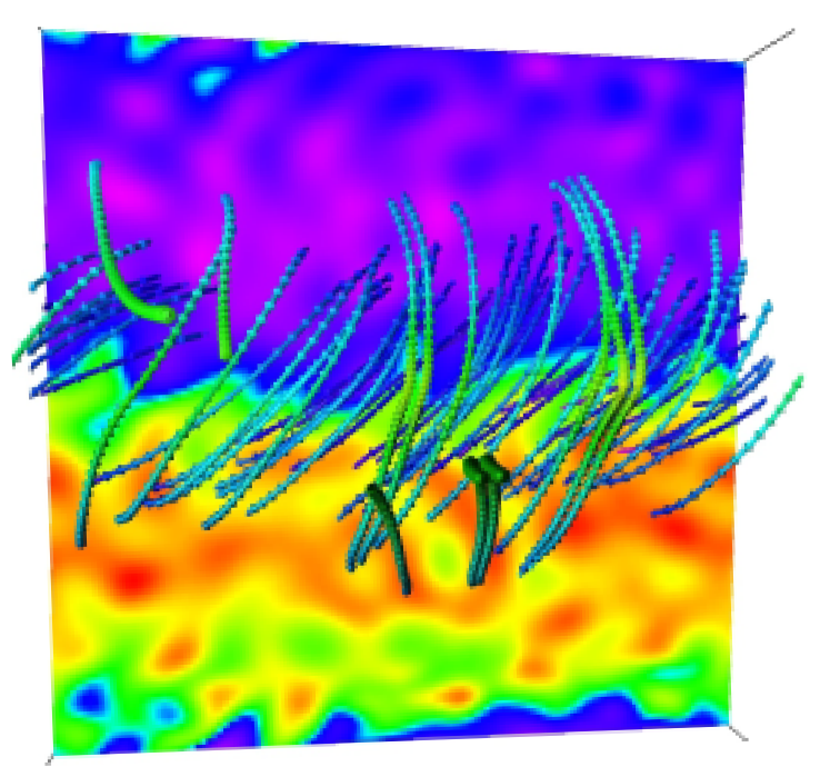
Figure 1: Three-dimensional visualization of the magnetic field viewed from above. The vertical magnetic field component is color-coded (light/yellow pointing upward and dark/blue pointing downward). Note that the field lines form a left-handed spiral over the scale of the domain, as expected for turbulence with positive helicity at small scales. The $x$-axis points to the right while the $y$-axis points upward. Adapted from Warnecke & Brandenburg (2010).

In Figure 1 we show the surface magnetic field of such a dynamo of the work of Warnecke & Brandenburg (2010). We show color-coded the vertical (line of sight) magnetic field component together with a perspective view of field lines in the volume above, which we shall refer to as the corona region. In addition to fluctuations, we can see a large-scale pattern of the field with a sinusoidal modulation in the $x$ direction and no systematic variation in the $y$ direction. The field lines in the corona region show a spiraling pattern corresponding to a left-handed spiral. This is because the helicity of the forcing function is in this model positive (right handed), so the resulting large-scale field must have helicity of the opposite sign.

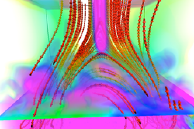
Figure 2: Magnetic field structure in the dynamo exterior. Field lines are shown in red and the modulus of the current density is shown in pink with semi-transparent opacity. Note the formation of a vertical current sheet above the arcade. Adapted from Warnecke & Brandenburg (2010).

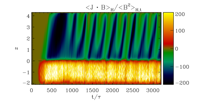
Figure 3: Dependence of $\langle\mbox{\boldmath$J$}{}\cdot\mbox{\boldmath$B$}{}\rangle_{\rm H}/\langle\mbox{\boldmath$B$}{}^{2}\rangle_{\rm H,t}$ on time and height. Dark/blue stands for negative and light/yellow for positive values. For this run the vertical extent of the domain is $-{\textstyle{2\over 3}}\pi\leq z\leq{\textstyle{4\over 3}}\pi$.

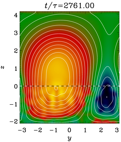
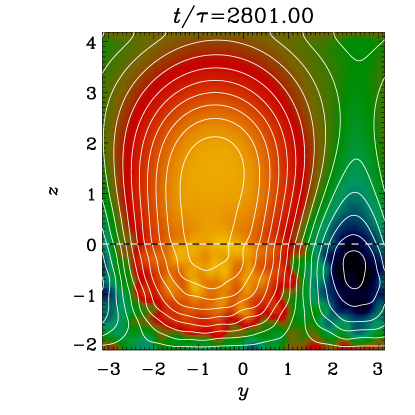
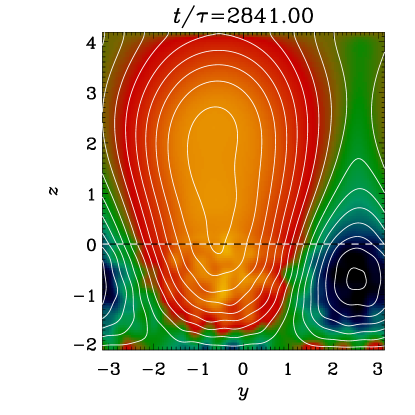
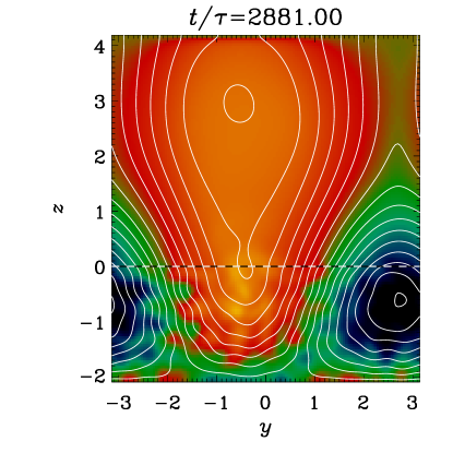
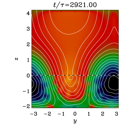
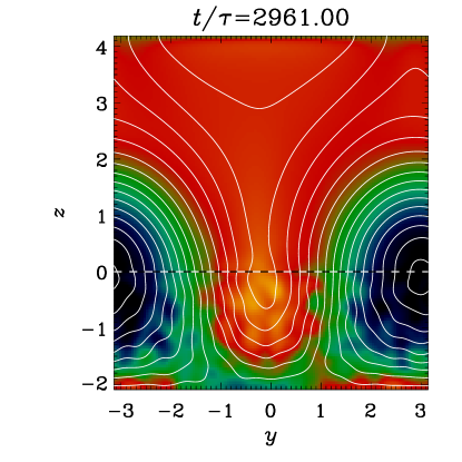
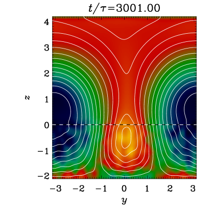
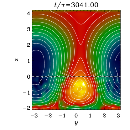
Figure 4: Time series of the formation of a plasmoid ejection. Contours of $\langle A_{x}\rangle_{x}$ are shown together with a color-scale representation of $\langle B_{x}\rangle_{x}$; dark/blue stands for negative and light/yellow for positive values, as in Figure 3. The contours of $\langle A_{x}\rangle_{x}$ correspond to field lines of $\langle\mbox{\boldmath$B$}{}\rangle_{x}$ in the $yz$ plane. The dashed horizontal lines show the location of the surface at $z=0$. For this run the vertical extent of the domain is $-{\textstyle{2\over 3}}\pi\leq z\leq{4\over 3}\pi$.

The large-scale magnetic field is essentially steady in the dynamo region and does not change its overall bipolar structure; see Figure 2 for a perspective view. However the magnetic field of the corona region shows a time-dependent oscillating structure associated with nearly regularly occurring ejection. The ejection events can be monitored in terms of the current helicity, $\mbox{\boldmath$J$}{}\cdot\mbox{\boldmath$B$}{}$, where $\mbox{\boldmath$J$}{}=\mbox{\boldmath$\nabla$}{}\times\mbox{\boldmath$B$}{}/\mu_{0}$ is the current density and $\mu_{0}$ the vacuum permeability. To compensate for the radial decline of $\mbox{\boldmath$J$}{}\cdot\mbox{\boldmath$B$}{}$, we have scaled it by $\langle\mbox{\boldmath$B$}{}^{2}\rangle_{H,t}$, which is here understood as a combined average over horizontal directions and over time. The result is shown in Figure 3.

It is remarkable that the field does not remain steady in the outer parts. This can be seen more clearly in a sequence of field line visualizations in Figure 4. Here, the magnetic field is averaged over the $x$-direction and we show $\langle B_{x}\rangle_{x}$ color coded together with magnetic field lines as contours of $\langle A_{x}\rangle_{x}$ in the $yz$-plane. Light/yellow shades correspond to positive values, the dark/blue to negative, similar to Figure 3. Note that a concentration in $B_{x}$ emerges from the lower region to the outer one. The magnetic field line surround the concentration and form a shape similar to plasmoid ejections, which are believed to be a two-dimensional model of producing CMEs (Ortolani & Schnack, 1993). At a time of $t/\tau=2881$ turnover times, the concentration is split into two parts, where the upper one leaves the domain through the upper boundary, while the lower one stays in the lower layer. Here, $\tau=(u_{\rm rms}k_{\rm f})^{-1}$ is the turnover time based on the forcing wavenumber $k_{\rm f}$ and $u_{\rm rms}$ is the root mean squared velocity averaged in the lower layer. At $t/\tau=3041$, the field line have formed an X-point in the center of the upper layer. In an X-point, field lines reconnect and release large amounts of energy through Ohmic heating. In the Sun these reconnection events are believed to trigger an eruptive flare, which can cause a CME. A similar behavior can also be seen in more realistic models in spherical geometry, as will be discussed in the next section.

3 Helicity reversals in spherical models

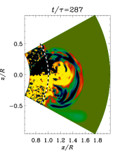
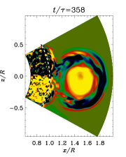
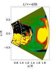
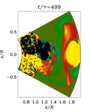
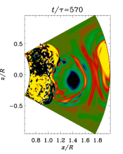
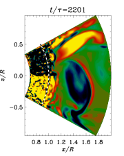
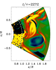
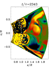
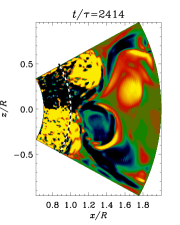
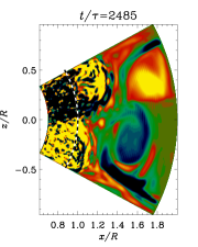
Figure 5: Time series of coronal ejections in spherical coordinates. The normalized current helicity, $\overline{\mbox{\boldmath$J$}{}\cdot\mbox{\boldmath$B$}{}}/\langle\overline{\mbox{\boldmath$B$}{}^{2}}\rangle_{t}$, is shown in a color-scale representation for different times; dark/blue stands for negative and light/yellow for positive values, as in Figure 3. The dashed lines show the location of the surface at $r^{2}=x^{2}+z^{2}=R^{2}$.

While similar ejection events are also seen in spherical geometry, a more surprising property is a reversal of the current helicity in the radial direction (Warnecke et al., 2011). In Figure 5 we show visualizations of $\mbox{\boldmath$J$}{}\cdot\mbox{\boldmath$B$}{}$ in meridional planes. The Figure shows two examples of coronal ejections which we found to be ejected from the dynamo region into the atmosphere. At $t/\tau=358$ we can identify a shape that is similar to that of the three-part structure of coronal mass ejections, observed on the Sun (Low, 1996). It consists of an arch of one sign of current helicity in front of a bulk of opposite sign and a cavity in between. As show in Figure 5, the ejection leaves the domain on the radial boundary and a new ejection of opposite sign occurs. We also see that in the dynamo region the current helicity is negative in the northern hemisphere and positive in the southern. This seems to be basically true also in the immediate proximity above the surface, but there is now an increasing tendency for the occurrence of magnetic helicity of opposite sign ahead of the ejecta. This seems to be associated with a redistribution of twist in the swept-up material. The current helicity is by far not always of the same sign, but both signs occur and there is only a slight preference of one sign over the other. This is seen more clearly in Figure 6, where we show a time series of $\mbox{\boldmath$J$}{}\cdot\mbox{\boldmath$B$}{}$ versus radial position $r/R$ and time $t/\tau$.

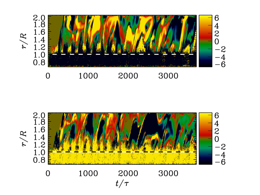
Figure 6: Dependence of the dimensionless ratio $\overline{\mbox{\boldmath$J$}{}\cdot\mbox{\boldmath$B$}{}}/\langle\overline{\mbox{\boldmath$B$}{}^{2}}\rangle_{t}$ on time and radius. The top panel shows a narrow band in $\theta$ in the northern hemisphere and the bottom one a narrow band in the southern hemisphere. Dark/blue stands for negative and light/yellow for positive values. The dashed horizontal lines show the location of the surface at $r=R$.

A time series of the normalized current helicity, $\overline{\mbox{\boldmath$J$}{}\cdot\mbox{\boldmath$B$}{}}/\langle\overline{\mbox{\boldmath$B$}{}^{2}}\rangle_{t}$, evaluated at radius $r=1.7\,R$ and $28^{\circ}$ latitude, is shown in Figure 7, where we also show their running means. It is now quite clear that on average the sign of current helicity has changed relative to what it was in the dynamo region. This is seen explicitly in a time-averaged plot of current helicity in the meridional plane (Figure 8).

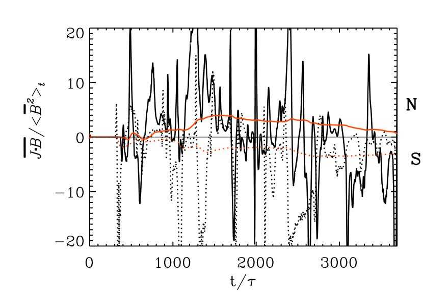
Figure 7: Dependence of the dimensionless ratio $\overline{\mbox{\boldmath$J$}{}\cdot\mbox{\boldmath$B$}{}}/\langle\overline{\mbox{\boldmath$B$}{}^{2}}\rangle_{t}$ on time at radius $r=1.7\,R$ and $28^{\circ}$ latitude. The solid line stands for the northern hemisphere and the dotted for the southern hemisphere. The red lines represent the cumulative mean for each hemisphere.

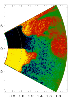
Figure 8: Current helicity averaged over time. Dark/blue corresponds to negative values, while the light/yellow corresponds to positive value, as in Figure 6. The dashed line show the location of the surface at $r^{2}=x^{2}+z^{2}=R^{2}$.

This reversal is significant because similar behavior has also been seen in recent measurements of the magnetic helicity spectrum in the solar wind (Brandenburg et al., 2011), but before showing the evidence for this, let us first discuss in more detail a similar diagnostics for the simulations. In Figure 9 we show the time variation of $B_{\theta}$ and $B_{\phi}$ and the magnetic helicity spectrum obtained from these time series. Unlike the solar wind, where a time series can be used to mimic a scan in distance space (the so-called Taylor hypothesis), this argument fails in the present case, because no wind is produced in the present model. There is only the pattern speed associated with the CMEs. Whether this is enough to motivate the use of the Taylor hypothesis is rather unclear. Nevertheless, there is a remarkable similarity with similar helicity spectra obtained for the solar wind; see Figure 10. In both cases, magnetic helicity has been obtained under the assumption of local isotropy of the turbulence. This means that one computes the one-dimensional magnetic energy $E_{\rm M}^{\rm 1D}(k_{R})$ and magnetic helicity spectra $H_{\rm M}^{\rm 1D}(k_{R})$ simply as

$$E_{\rm M}(k_{R})=|\hat{\mbox{\boldmath$B$}{}}|^{2}/\mu_{0},\quad H_{\rm M}^{\rm 1D}(k_{R})=4\,{\rm Im}(\hat{B}_{\theta}\hat{B}_{\phi}^{\star})/k_{R},$$ (1)

where $k_{R}$ is the component of the wave vector in the radial direction. Here, a hat denotes Fourier transformation and an asterisk complex conjugation. These are the equations used by Matthaeus et al. (1982) who applied such an analysis to data from Voyager 2. Since Voyager 2 flew close to the ecliptic, the magnetic helicity is dominated by fluctuations. This is why Brandenburg et al. (2011) applied this analysis to Ulysses data, where a net magnetic helicity was seen for the first time. An important advantage of Ulysses over Voyager 1 and 2 is the high angle with the ecliptic. So, only with Ulysses we can measure the magnetic helicity far away from the ecliptic in both hemispheres of the heliosphere.

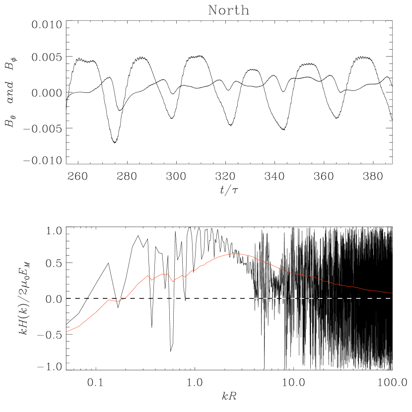
Figure 9: Helicity in the northern outer atmosphere. The values are written out at the point, $r=1.5\,R$, $90^{\circ}-\theta=17^{\circ}$, and $\phi=9^{\circ}$. Top panel: Phase relation between the toroidal $B_{\phi}$ and poloidal $B_{\theta}$ field, plotted over time $t/\tau$. Bottom panel: Helicity $H(k)$ is plotted over normalized wave number $kR$. The helicity is calculated with the Taylor hypothesis using the Fourier transformation of the poloidal and toroidal field. Adapted from Warnecke et al. (2011).

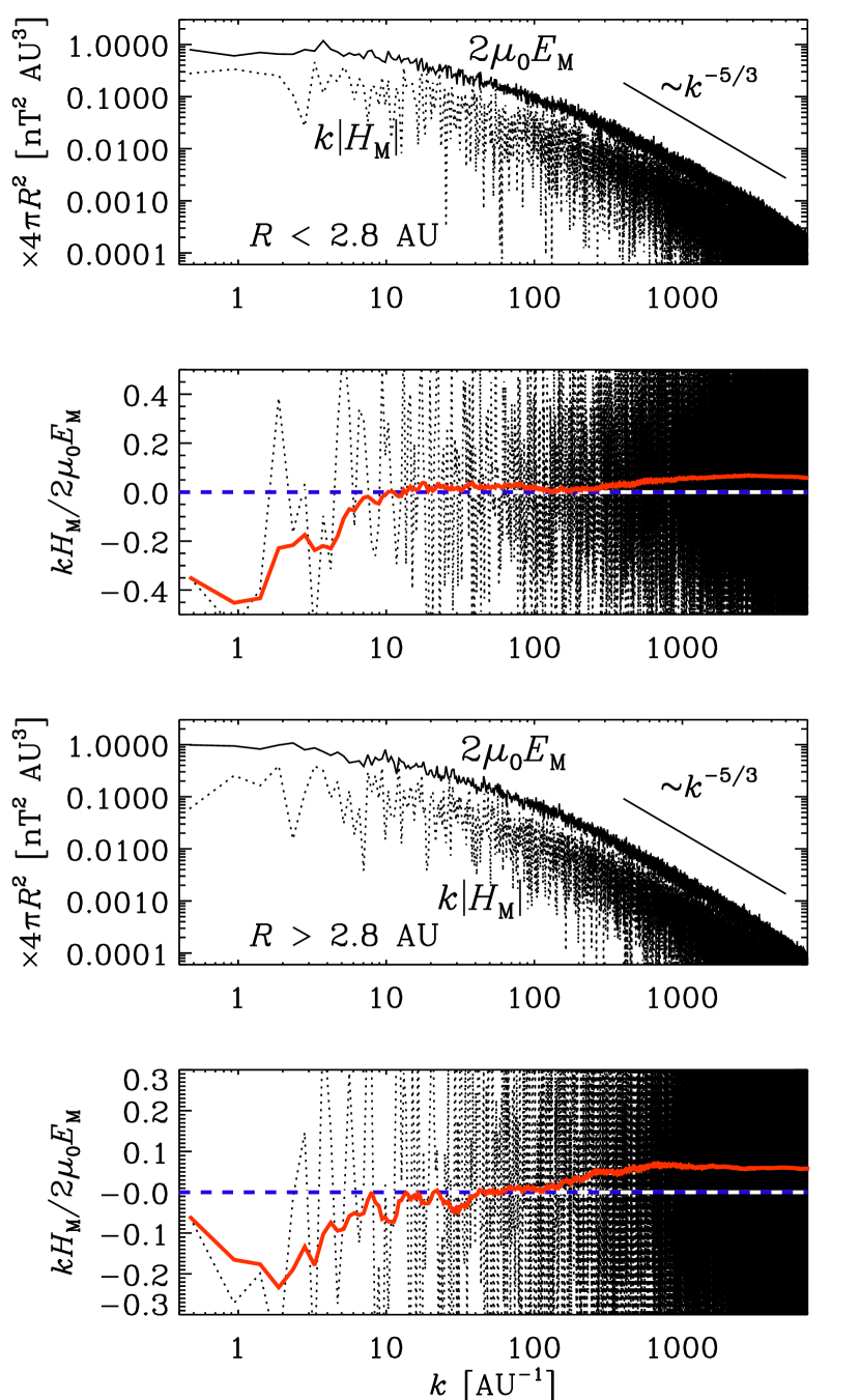
Figure 10: Magnetic energy and helicity spectra, $2\mu_{0}E_{\rm M}(k)$ and $k|H_{\rm M}(k)|$, respectively, for two separate distance intervals (first and third panels). Furthermore, both spectra are scaled by $4\pi R^{2}$ before averaging within each distance interval above and below $2.8\,{\rm AU}$, respectively. The relative magnetic helicity, $kH_{\rm M}(k)/2\mu_{0}E_{\rm M}(k)$, is plotted separately (second and fourth panels) together with its cumulative average starting from the low wavenumber end. The zero line is shown in dashed. Adapted from Brandenburg et al. (2011).

Table 1: Distribution of magnetic helicity at large and small scales both in the dynamo region close to or below the surface and the corona region, solar wind or the exterior of the dynamo.

Magnetic helicity Large scales small scales Dynamo region, interior $+$ $-$ Corona region, solar wind, exterior $-$ $+$

What we see both in the simulations and in the solar wind is that there is magnetic helicity of opposite sign at large and small scales. However, it is exactly the other way around than what is found in the corona region; see Table 1. To understand the reason for this, we need to consider the equations for the production of magnetic helicity at large and small length scales. As will be argued in Section 4, the mechanism that sustains negative small-scale helicity in the north is turned off in the solar wind, and there is just the effect of turbulent magnetic diffusion which contributes with opposite sign. By contrast, inside the dynamo region, turbulent diffusion is subdominant, because otherwise no large-scale magnetic field would be generated. However, in the wind we do not expect the dynamo to be exited, so here diffusion dominates.

4 Connection with earlier dynamo models

The purpose of this section is to make contact with dynamo theory and to understand more quantitatively why the magnetic helicity reverses sign with radius. In essence, we argue that the profile of magnetic helicity density must have a positive radial gradient to maintain a negative diffusive magnetic helicity flux and that this is the reason for the magnetic helicity to change from a negative sign to a positive one at some radius in the northern hemisphere.

We begin by discussing the magnetic helicity equation. The magnetic helicity density is $h=\mbox{\boldmath$A$}{}\cdot\mbox{\boldmath$B$}{}$, where $\mbox{\boldmath$B$}{}=\mbox{\boldmath$\nabla$}{}\times\mbox{\boldmath$A$}{}$ is the magnetic field expressed in terms of the magnetic vector potential $A$ which, in the Weyl gauge, satisfies $\partial\mbox{\boldmath$A$}{}/\partial t=\mbox{\boldmath$U$}{}\times\mbox{\boldmath$B$}{}-\eta\mu_{0}\mbox{\boldmath$J$}{}$. The evolution equation for $\mbox{\boldmath$A$}{}\cdot\mbox{\boldmath$B$}{}$ is then

$${\partial\over\partial t}\mbox{\boldmath$A$}{}\cdot\mbox{\boldmath$B$}{}=-2\eta\mu_{0}\mbox{\boldmath$J$}{}\cdot\mbox{\boldmath$B$}{}-\mbox{\boldmath$\nabla$}{}\cdot\mbox{\boldmath$F$}{},$$ (2)

where $F$ is the magnetic helicity flux. Next, we define large-scale fields as averaged quantities, denoted by an overbar, and small-scale fields as the residual, denoted by lower case characters, so the magnetic field can be split into two contributions via $\mbox{\boldmath$B$}{}=\overline{\mbox{\boldmath$B$}}{}+\mbox{\boldmath$b$}{}$. Likewise, $\mbox{\boldmath$A$}{}=\overline{\mbox{\boldmath$A$}}{}+\mbox{\boldmath$a$}{}$, $\mbox{\boldmath$J$}{}=\overline{\mbox{\boldmath$J$}}{}+\mbox{\boldmath$j$}{}$, and $\mbox{\boldmath$U$}{}=\overline{\bm{U}}+\mbox{\boldmath$u$}{}$. The evolution equation for the mean magnetic helicity density $\overline{h}=\overline{\mbox{\boldmath$A$}{}\cdot\mbox{\boldmath$B$}{}}$ is given by

$${\partial\over\partial t}\overline{\mbox{\boldmath$A$}{}\cdot\mbox{\boldmath$B$}{}}=-2\eta\mu_{0}\overline{\mbox{\boldmath$J$}{}\cdot\mbox{\boldmath$B$}{}}-\mbox{\boldmath$\nabla$}{}\cdot\overline{\mbox{\boldmath$F$}}{}.$$ (3)

To determine the magnetic helicity density of the mean field, $\overline{h}_{\rm m}=\overline{\mbox{\boldmath$A$}}{}\cdot\overline{\mbox{\boldmath$B$}}{}$, we use the averaged induction equation in the Weyl gauge, $\partial\overline{\mbox{\boldmath$A$}}{}/\partial t=\overline{\bm{U}}\times\overline{\mbox{\boldmath$B$}}{}+\overline{\mbox{\boldmath$u$}{}\times\mbox{\boldmath$b$}{}}-\eta\mu_{0}\overline{\mbox{\boldmath$J$}}{}$, so that

$${\partial\over\partial t}\overline{\mbox{\boldmath$A$}}{}\cdot\overline{\mbox{\boldmath$B$}}{}=2\,\overline{\mbox{\boldmath$u$}{}\times\mbox{\boldmath$b$}{}}\cdot\overline{\mbox{\boldmath$B$}}{}-2\eta\mu_{0}\overline{\mbox{\boldmath$J$}}{}\cdot\overline{\mbox{\boldmath$B$}}{}-\mbox{\boldmath$\nabla$}{}\cdot\overline{\mbox{\boldmath$F$}}_{\rm m}{}.$$ (4)

The magnetic helicity equation for the fluctuating field, $\overline{h}_{\rm f}=\overline{h}-\overline{h}_{\rm m}=\overline{\mbox{\boldmath$a$}{}\cdot\mbox{\boldmath$b$}{}}$, takes then the form

$${\partial\over\partial t}\overline{\mbox{\boldmath$a$}{}\cdot\mbox{\boldmath$b$}{}}=-2\,\overline{\mbox{\boldmath$u$}{}\times\mbox{\boldmath$b$}{}}\cdot\overline{\mbox{\boldmath$B$}}{}-2\eta\mu_{0}\overline{\mbox{\boldmath$j$}{}\cdot\mbox{\boldmath$b$}{}}-\mbox{\boldmath$\nabla$}{}\cdot\overline{\mbox{\boldmath$F$}}_{\rm f}{},$$ (5)

so that the sum of Equations (4) and (5) gives Equation (3). Here, the total magnetic helicity flux consists of contribution from mean and fluctuating fields, denoted by subscripts m and f, respectively, i.e., $\overline{\mbox{\boldmath$F$}}_{\rm m}{}+\overline{\mbox{\boldmath$F$}}_{\rm f}{}=\overline{\mbox{\boldmath$F$}}{}$. Note that, even in the limit $\eta\to 0$ and in the absence of fluxes, magnetic helicity at large and small scales is not conserved individually, but there can be an exchange of magnetic helicity between scales.

A note regarding the gauge-dependence is here in order. Obviously, Equation (5) depends on the gauge choice for $a$. However, if we are in a steady state, and if $\overline{h}_{\rm f}$ also happens to be steady (which is not automatically guaranteed), then we have

$$\mbox{\boldmath$\nabla$}{}\cdot\overline{\mbox{\boldmath$F$}}_{\rm f}{}=-2\,\overline{\mbox{\boldmath$u$}{}\times\mbox{\boldmath$b$}{}}\cdot\overline{\mbox{\boldmath$B$}}{}-2\eta\mu_{0}\overline{\mbox{\boldmath$j$}{}\cdot\mbox{\boldmath$b$}{}},$$ (6)

and since the right-hand side of this equation is manifestly gauge-invariant, $\mbox{\boldmath$\nabla$}{}\cdot\overline{\mbox{\boldmath$F$}}_{\rm f}{}$ must also be gauge-invariant. This property was used in earlier work of Mitra et al. (2010), Hubbard & Brandenburg (2010) and Warnecke et al. (2011) to determine the scaling of $\overline{\mbox{\boldmath$F$}}_{\rm f}{}$ with $\mbox{\boldmath$\nabla$}{}\overline{h}_{\rm f}$ and thus the turbulent diffusion coefficient $\kappa_{h}$. In addition, if there is sufficient scale separation between large and small scales, which is typically the case in the nonlinear regime at the end of the inverse cascade process (Brandenburg, 2001), then $\overline{h}_{\rm f}$ can be expressed as a density of linkages, which is itself manifestly gauge-independent (Subramanian & Brandenburg, 2006). This property then also applies to the flux $\overline{\mbox{\boldmath$F$}}_{\rm f}{}$.

The correlation $\overline{\mbox{\boldmath$u$}{}\times\mbox{\boldmath$b$}{}}$ is known to have two contributions, one proportional to $\overline{\mbox{\boldmath$B$}}{}$ with a pseudo-tensor in front of it (the $\alpha$ effect, responsible for large-scale field generation), and one proportional to $\overline{\mbox{\boldmath$J$}}{}$ with a coefficient $\eta_{\rm t}$ in front of it that corresponds to turbulent diffusion, i.e.,

$$\overline{\mbox{\boldmath$u$}{}\times\mbox{\boldmath$b$}{}}=\alpha\overline{\mbox{\boldmath$B$}}{}-\eta_{\rm t}\mu_{0}\overline{\mbox{\boldmath$J$}}{},$$ (7)

where we have again assumed isotropy. The reason why the mean magnetic helicity density of the small-scale field is negative in the north is because $\alpha>0$ in the north (e.g. Krause and Rädler, 1980), producing therefore negative magnetic helicity at a rate $-2\alpha\overline{\mbox{\boldmath$B$}}{}^{2}<0$ for small-scale fields and $+2\alpha\overline{\mbox{\boldmath$B$}}{}^{2}>0$ for large-scale fields, so that their sum vanishes. There is also turbulent magnetic diffusion which reduces this effect, because $\eta_{\rm t}>0$ and $\overline{\mbox{\boldmath$J$}}{}\cdot\overline{\mbox{\boldmath$B$}}{}>0$ in the north. In the solar wind no new magnetic field is generated, so turbulent magnetic diffusion could now dominate and might thus explain a reversal of magnetic helicity density (Brandenburg et al., 2011).

Support for a reversal of the sign of magnetic helicity was first seen in dynamo simulations with magnetic helicity flux in the exterior. In Figure 11 we show a representation of magnetic helicity density of small-scale fields $\overline{h}_{\rm f}=\overline{\mbox{\boldmath$a$}{}\cdot\mbox{\boldmath$b$}{}}$ versus $z$ and $t$ for a model similar to that of Brandenburg et al. (2009), but where the magnetic helicity flux is caused by a wind that is then running into a shock where the flux is artificially suppressed at height $z=3H$. This figure shows that there is a clear segregation of negative and positive small-scale magnetic helicity in the dynamo regime and the exterior, respectively.

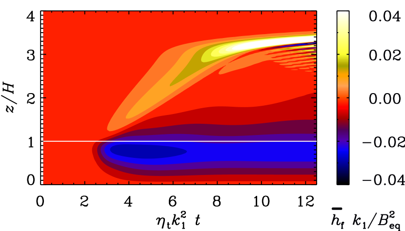
Figure 11: $zt$ diagrams of $\overline{h}_{\rm f}$ for an $\alpha^{2}$ dynamo with a wind which stops all of a sudden at $z/H=3$. The white horizontal line marks the location $z=H$. Light/yellow shades indicate positive values and dark/blue shades indicate negative values.

In our description above we have suggested that the magnetic helicity production balances the $\partial\overline{\mbox{\boldmath$a$}{}\cdot\mbox{\boldmath$b$}{}}/{\rm d}{}t$ term, but this cannot be true in the steady state. Instead, it must be the divergence of the magnetic helicity flux, $\mbox{\boldmath$\nabla$}{}\cdot\overline{\mbox{\boldmath$F$}}_{\rm f}{}$. Let us assume that $\overline{\mbox{\boldmath$F$}}_{\rm f}{}$ can be approximated by a Fickian diffusion law, i.e., $\overline{\mbox{\boldmath$F$}}_{\rm f}{}=-\kappa_{h}\mbox{\boldmath$\nabla$}{}\overline{h}_{\rm f}$. Simulations have suggested that $\kappa_{h}/\eta_{\rm t}$ is around 0.3 (Mitra et al., 2010; Hubbard & Brandenburg, 2010; Warnecke et al., 2011). Thus, balancing now the source $S(z)\equiv-2\alpha\overline{\mbox{\boldmath$B$}}{}^{2}+2\eta_{\rm t}\mu_{0}\overline{\mbox{\boldmath$J$}{}\cdot\mbox{\boldmath$B$}{}}$ against the divergence of the flux of magnetic helicity at small scales, we have, in a one-dimensional model (neglecting the molecular diffusion term, $2\eta\mu_{0}\overline{\mbox{\boldmath$j$}{}\cdot\mbox{\boldmath$b$}{}}$):

$$S(z)=-\kappa_{h}{{\rm d}{}^{2}\overline{h}_{\rm f}\over{\rm d}{}z^{2}}.$$ (8)

Taking as an example a source where $S(z)/\kappa_{h}=-1$ in the dynamo interior ($z<0$), and $S(z)=0$ in $z>0$, we have a family of solutions of Equation (8) that only differ in an undetermined integration constant corresponding to a constant offset in the flux; see the second panel of Figure 12. The solutions for which the magnetic helicity flux, $-\kappa_{h}{\rm d}{}\overline{h}_{\rm f}/{\rm d}{}z$, is negative in the exterior are those for which $\overline{h}_{\rm f}$ reaches an extremum below the surface. This seems to be what happens both in simulations and in the solar wind. We can thus conclude that the reason for a sign change is not a dominance of turbulent diffusion in the solar wind, but just the possibility of the magnetic helicity density reaching an extremum below the surface (dashed red and solid black lines in Figure 12), not at the surface (dotted blue lines).

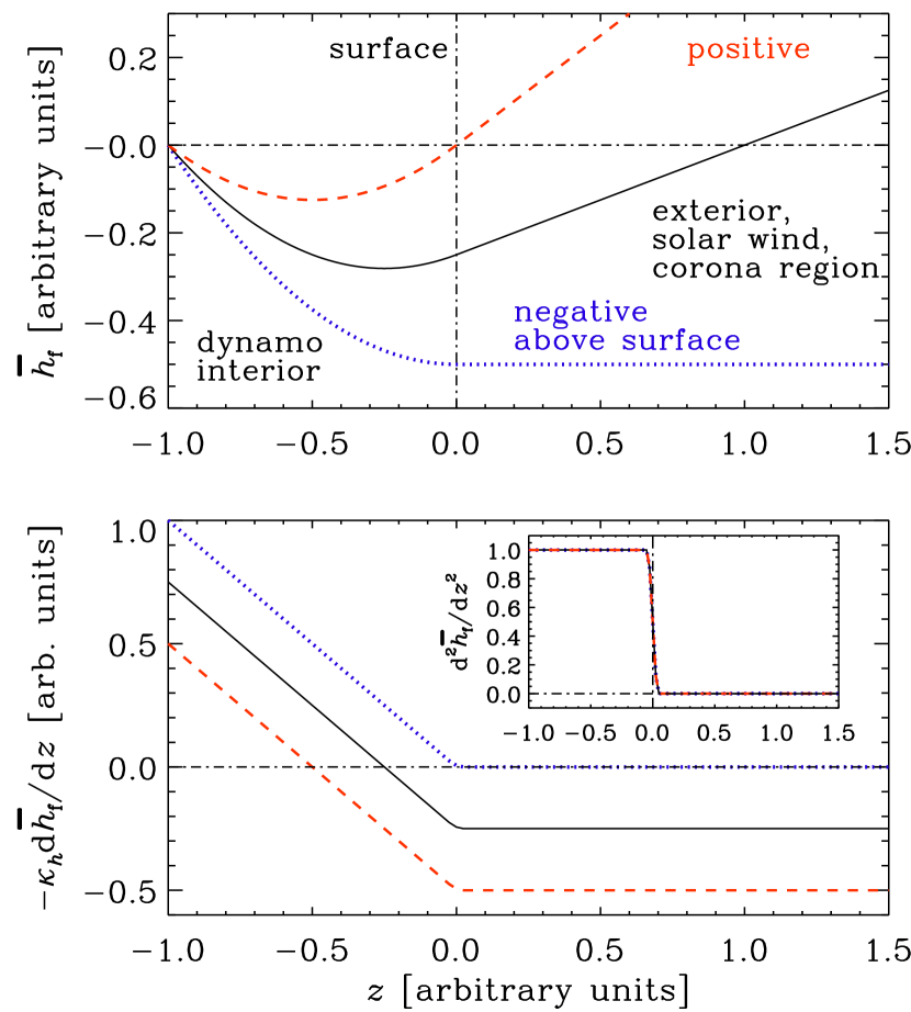
Figure 12: Sketch showing possible solutions $\overline{h}_{\rm f}(z)$ (upper panel) to Equation (8) with $S={\rm const}{}=-1$ in $z<0$ and $S=0$ in $z>0$. The red (dashed) and black (solid) lines show solutions for which the magnetic helicity flux ($-\kappa_{h}{\rm d}{}\overline{h}_{\rm f}/{\rm d}{}z$, see lower panel) is negative in the exterior. This corresponds to the case observed in the Sun. The blue (dotted) line shows the case, where the magnetic helicity flux is zero above the surface and therefore do not reverse the sign of $\overline{h}_{\rm f}(z)$ in the exterior.

5 Conclusions

As we have seen in the present paper, magnetic twist (or helicity) plays an important role for the solar dynamo (Brandenburg, 2001; Blackman & Brandenburg, 2002) and for producing eruptions of the form of CMEs (Low, 1996, 2001). The recent work of Warnecke & Brandenburg (2010) and Warnecke et al. (2011) tries to combine both aspects into one. Although the models are still rather unrealistic in many respects, they have already now led to useful insights into the interplay between dynamo models and solar wind turbulence. In particular, they have allowed us to understand the properties of magnetic helicity fluxes. We have confirmed that the hemispheric sign rule of magnetic helicity does not extend unchanged into the interplanetary space, but we have now shown that it must flip sign somewhere above the solar surface. On the other hand, Bothmer & Schwenn (1998) found that the magnetic clouds follow Hale’s polarity and that the sign of the magnetic helicity is the same as in the interior. However, this result is not based on rigorous statistics.

Future work in this direction should include more realistic modeling of the solar convection zone. Preliminary work in this direction is already underway (Warnecke et al., 2012). Furthermore, it will be necessary to allow for the development of a proper solar wind from the dynamo region. One of the difficulties here is that, if the critical point is assumed to be too close to the solar surface, which would be computationally convenient because it would allow us to use a smaller domain, the mass loss rate would be rather high and could destroy the dynamo. In future work we will be trying to strike an appropriate compromise that will allow us to study the qualitatively new effects emerging from this.

$Header: /var/cvs/brandenb/tex/joern/namur/paper.tex,v 1.62 2012-07-15 21:12:36 joern Exp $