Quench dynamics of the Tomonaga-Luttinger model with momentum dependent interaction

Abstract

We study the relaxation dynamics of the one-dimensional Tomonaga-Luttinger model after an interaction quench paying particular attention to the momentum dependence of the two-particle interaction. Several potentials of different analytical form are investigated all leading to universal Luttinger liquid physics in equilibrium. The steady-state fermionic momentum distribution shows universal behavior in the sense of the Luttinger liquid phenomenology. For generic regular potentials the large time decay of the momentum distribution function towards the steady-state value is characterized by a power law with a universal exponent which only depends on the potential at zero momentum transfer. A commonly employed ad hoc procedure fails to give this exponent. Besides quenches from zero to positive interactions we also consider abrupt changes of the interaction between two arbitrary values. Additionally, we discuss the appearance of a factor of two between the steady-state momentum distribution function and the one obtained in equilibrium at equal two-particle interaction.

1 Introduction

The experimental progress in controlling and manipulating cold atomic gases [1], which in certain parameter regimes form strongly correlated quantum many-body systems, led to tremendous activities with the final goal of theoretically understanding the quench dynamics in such systems (for a recent review, see Ref. [2]). In a sudden quench at least one parameter of a given Hamiltonian is switched abruptly at time $t=0$—the Hamiltonian before the quench is $H_{\rm i}$, the one afterwards $H_{\rm f}$. At $t=0$ the system is assumed to be in the ground state (we consider temperature $T=0$) of $H_{\rm i}$ and the time evolution for $t>0$ is performed with respect to $H_{\rm f}$. We here study ’global’ quenches of the two-particle interaction.

Describing the time evolution of a correlated quantum system out of a nonequilibrium state poses a formidable challenge. It is reasonable to consider the case of one-dimensional (1d) systems first, as in 1d a variety of analytical as well as numerical methods exist which allow for controlled access to equilibrium correlation effects in specific models [3, 4, 5, 6]. Several of those techniques were recently extended to study the nonequilibrium problem at hand [7, 8, 9, 10, 11, 12, 13, 14, 15, 16]. Furthermore, in 1d chains virtually all many-body states of matter of current interest, such as Mott insulators, superfluids, superconductors and charge- as well as spin-density-wave states can be realized. Quenching between these states is expected to be particularly interesting.

We here focus on fermionic systems. Even if the system stays metallic in the presence of two-particle interactions the Fermi liquid concept breaks down. Instead a wide class of 1d models shows Luttinger liquid (LL) behavior on low-energy scales [3, 4, 5]. Equilibrium LL physics is characterized by the ’universal’ power-law decay of certain correlation functions in space-time with exponents which for spinless and spin-rotational invariant models can all be expressed in terms of a single number $K$. This LL parameter in turn is a function of the microscopic details of the model considered, in particular the strength of the two-particle interaction. For noninteracting fermions $K=1$ and $0<K<1$ for repulsive ones; the case we focus on.

The Tomonaga-Luttinger (TL) model is the exactly solvable effective low-energy fixed point model of the LL universality class [17, 18, 3, 4, 5]. It thus plays a similar role as the free Fermi gas in Fermi liquid theory. The model has two strictly linear branches of right- and left-moving fermions and two-particle scattering is restricted to processes with small momentum transfer $|q|\ll k_{\rm F}$, with the Fermi momentum $k_{\rm F}$. These processes as well as the kinetic energy can be written as quadratic forms of the densities of right- and left-moving fermions which obey bosonic commutation relations. In most calculations the momentum dependence of the low-momentum scattering processes $g_{2}$ and $g_{4}$ (in the so-called g-ology classification [18]; see below) are (partially) neglected and momentum integrals are regularized in the ultraviolet introducing a convenient cutoff ’by hand’.

In the bosonization procedure the interacting Fermi system is mapped onto a model of free bosons. The time evolution of the latter is trivial and the dynamics of correlation functions of the fermionic densities (at small momenta) after an interaction quench can be accessed directly. In addition, the fermionic field operator can be written as a (highly nonlinear) function of the bosonic eigenmodes $\alpha_{n}^{({\dagger})}$ [17, 3, 4, 5] such that the time evolution of fermionic correlation functions can be computed exactly as well. The TL model thus constitutes an ideal play ground for studying the dynamics resulting from an interaction quench.

The time evolution of the fermionic single-particle Green function $G_{t}(x)=\left<\psi^{\dagger}(x)\psi(0)\right>_{\rho(t)}$ as well as the density correlation function (at small momenta) after suddenly turning on the interaction in the spinless TL model was first studied in Ref. [19]. Here $\psi^{({\dagger})}(x)$ denotes the field operator and $\left<\ldots\right>_{\rho(t)}$ the expectation value with respect to the time-dependent density matrix $\rho(t)$. In Ref. [19] it was found that at large $t$ the Green function approaches a time-independent stationary limit. At $T=0$ the stationary Green function shows power-law behavior as a function of the position $x$ with a $K$ dependent exponent. Power-law decay of $\lim_{t\to\infty}G_{t}(x)=G^{\rm st}(x)$ at large $|x|$ translates into a typical LL power-law behavior of the stationary fermionic momentum distribution function close to $k_{\rm F}$, $|n^{\rm st}(k)-1/2|\sim|k-k_{\rm F}|^{\gamma_{\rm st}}$, with $\gamma_{\rm st}$ being a function of $K$ and thus depending on the strength of the interaction. Interestingly, the steady-state exponent $\gamma_{\rm st}$ differs from the one of the ground-state momentum distribution function $\gamma_{\rm gs}$ at the same interaction strength. For finite times $n(k,t)$ has a Fermi liquid-like jump at $k_{\rm F}$, with a $Z$-factor which vanishes as a power law in $t$: $Z\sim t^{-\gamma_{\rm st}}$. Further aspects of the quench dynamics of the TL model or closely related ones were discussed in Refs. [20, 21, 22, 23, 24].

In Ref. [19] an ad hoc ultraviolet regularization was used. It is widely believed that (partially) neglecting the momentum dependence of the interaction and regularizing momentum integrals as convenient has no effect on the low-energy equilibrium physics of the TL model. This is indeed correct if all energy scales are sent to zero [25]. The such obtained results for the dependence of power-law exponents of specific correlation functions on the LL parameter $K$ become universal and are valid for all models falling into the LL universality class. It is however questionable if the same reasoning holds when considering quenches. High energy processes and thus the full momentum dependence of the two-particle interaction might matter in this nonequilibrium situation. To investigate this issue we keep the momentum dependence of the $g_{2}$ and $g_{4}$ processes—rendering any ad hoc ultraviolet regularization superfluous [25]—and consider interaction potentials of different analytical form. We exactly compute $G_{t}(x)$ and its Fourier transform, the fermionic momentum distribution function $n(k,t)$, of the spinless TL model after a quench out of the noninteracting ground state. We first show that independent of the details of the momentum dependence of the interaction the steady-state momentum distribution as a function of $k$ is characterized by a power-law nonanalyticity at $k_{\rm F}$ with the exponent $\gamma_{\rm st}(K)$. The LL parameter $K$ is a function of the potential at zero momentum transfer only. Therefore $n^{\rm st}(k)$ of the TL model is universal in the LL sense. Similarly, the $Z$-factor shows a universal power-law decay in time. We then proceed and show that for generic regular potentials also the asymptotic time dependence of $n(k,t)$ has universal aspects. For fixed $k\neq k_{\rm F}$ we find a power-law decay towards the steady-state value as a function of $t$ with the $k$-independent exponent $1+\gamma_{\rm st}$. The ad hoc procedure instead gives the exponent $1+3\gamma_{\rm st}/2$ and is thus insufficient for studies of the generic dynamics. The power-law decay is overlaid by an oscillation with a frequency which depends on the momentum $k$ considered as well as the momentum dependence of the potential. In addition, we investigate a box shaped (in momentum space) potential and show that the asymptotic dynamics is dominated by its discontinuity leading to a power-law decay with exponent $1$ (independent of the interaction strenght). We raise the question if the universality in the steady state as well as the large time dynamics of the TL model after an interaction quench extend to other models of the (equilibrium) LL universality class. Besides quenches from zero to positive interactions we briefly consider quenches between two interactions of arbitrary strength.

Our paper is organized as follows. In Sec. 2 we present the model and give details on how to compute the single-particle Green function after a quench. Particular emphasis is put on the ultraviolet regularization by momentum dependent two-particle potentials. Different model potentials are introduced. In Sec. 3 we compute and compare the steady-state and equilibrium Green and momentum distribution functions. For small interactions they differ by a factor of two which was earlier discussed in the context of pre-thermalized states [26, 27, 28]. In Sec. 4 we present our results for $n(k,t)$ and show that they partly depend on the form of the potential considered. We also discuss results for the standard ad hoc regularization. Finally, our findings are summarized in Sec. 5.

2 Model and methods

2.1 The Tomonaga-Luttinger model and bosonization

The interaction energy of a translational invariant system (periodic boundary conditions) of 1d spinless fermions interacting via a potential which only depends on the distance between the two scattering particles can be written as

$$H_{\rm pot}=\frac{1}{L}\,\sum_{n>0}v(q_{n})\rho_{n}\rho_{-n}+h_{1}(N)\;,\;\;\;q_{n}=\frac{2\pi}{L}\,n\;,\;\;\;n\in{\mathbb{Z}}\;,$$ (1)

with the density operator

$$\rho_{n}=\sum_{m}c_{m}^{\dagger}c_{m+n}$$ (2)

and the Fourier transform $v(k)$ of the two-particle potential $V(x)$. Here the $c_{n}^{({\dagger})}$ denote fermionic momentum space annihilation (creation) operators, $h_{1}(N)$ contains terms which depend on the particle number operator $N$, and $L$ is the length of the system. After linearization of the single-particle dispersion around the two Fermi points at $\pm k_{\rm F}$ the kinetic energy reads

$$\mbox{}H_{\rm kin}=\sum_{n>0}v_{\rm F}(k_{n}-k_{\rm F})c_{n,+}^{\dagger}c_{n,+}+\sum_{n<0}(-v_{\rm F})(k_{n}+k_{\rm F})c_{n,-}^{\dagger}c_{n,-}+h_{2}(N)\;,$$ (3)

where we already introduced independent right- ($c_{n>0,+}$) and left-moving ($c_{n<0,-}$) fermions [5]. The Fermi velocity is denoted by $v_{\rm F}$. In the next step one supplements the Hilbert space of the right movers by states with negative momenta and the one of left movers by states with positive momenta. The linearization and addition of states does not change the equilibrium low-energy physics. From now on we drop terms containing $N$ as they are irrelevant for our considerations. The kinetic energy $H_{\rm kin}$ can then be written as a quadratic form in the densities $\rho_{n,\pm}$ of the right and left movers defined in analogy to Eq. (2) [5]. With

$$b_{n}=\frac{1}{\sqrt{|n|}}\left\{\begin{array}[]{cc}\rho_{n,+}&\mbox{for}\;n>0\\ \rho_{n,-}&\mbox{for}\;n<0\end{array}\right.\;,$$ (6)

one obtains

$$H_{\rm kin}=\sum_{n\neq 0}v_{\rm F}|k_{n}|b_{n}^{\dagger}b_{n}\;.$$ (7)

The $b_{n}^{({\dagger})}$ obey the standard bosonic commutation relations. Replacing $\rho_{n}\to\rho_{n,+}+\rho_{n,-}$ in Eq. (1), using Eq. (6) we obtain the Hamiltonian of the TL model

$$\mbox{}H_{\rm TL}=\sum_{n>0}\left[k_{n}\left(v_{\rm F}+\frac{v(k_{n})}{2\pi}\right)\left(b_{n}^{\dagger}b_{n}+b_{-n}^{\dagger}b_{-n}\right)+k_{n}\frac{v(k_{n})}{2\pi}\left(b_{n}^{\dagger}b_{-n}^{\dagger}+b_{-n}b_{n}\right)\right]\;.$$ (8)

Distinguishing between intra- and inter-branch scattering processes one often replaces the potential $v(k)$ in the first term by a function $g_{4}(k)$ and the one in the second by an independent function $g_{2}(k)$ [18]. For simplicity we here refrain from doing so and assume $g_{2}(k)=g_{4}(k)=v(k)$. This has no effect on our main results.

2.2 Eigenmodes and dynamics

By a Bogoliubov transformation the ’bosonized’ Hamiltonian $H_{\rm TL}$ can straightforwardly be diagonalized

$$H_{\rm TL}=\sum_{n\neq 0}\omega(k_{n})\,\alpha_{n}^{\dagger}\alpha_{n}+E_{\rm gs}$$ (9)

by introducing the eigenmodes

$$\alpha_{n}=c(k_{n})b_{n}-s(k_{n})b_{-n}^{\dagger}\;\;\Leftrightarrow\;\;b_{n}=c(k_{n})\alpha_{n}+s(k_{n})\alpha_{-n}^{\dagger}$$ (10)

with

$$s^{2}(k_{n})=\frac{1}{2}\left[\frac{1+\hat{v}(k_{n})/2}{\sqrt{1+\hat{v}(k_{n})}}-1\right]\;,\;\;c^{2}(k_{n})=1+s^{2}(k_{n})\;,$$

$$\omega(k_{n})=v_{\rm F}\,|k_{n}|\,\sqrt{1+\hat{v}(k_{n})}\;,\;\;\hat{v}(k_{n})=\frac{v(k_{n})}{\pi v_{\rm F}}\;.$$ (11)

In the noninteracting limit $s^{2}(k_{n})\to 0$ and $\omega(k_{n})\to v_{\rm F}|k_{n}|$. For physical reasons the Fourier transform $v(q)$ of the two-particle potential must vanish on a characteristic scale denoted by $q_{\rm c}$. This implies

$$\lim_{k\to\infty}s^{2}(k)=0\;,\;\;\;\;\;\lim_{k\to\infty}c^{2}(k)=1\;,\;\;\;\;\;\lim_{k\to\infty}\frac{\omega(k)}{|k|}=v_{\rm F}\;.$$ (12)

The LL parameter $K$ of the TL model is

$$K=\left[1+\hat{v}(0)\right]^{-1/2}\;.$$ (13)

It thus only depends on the (dimensionless; see Eq. (11)) potential at momentum $q=0$. This shows that the TL model is a LL with $0<K<1$ only if $\hat{v}(0)>0$; we here focus on two-particle potentials with this property. Using Eq. (11) one finds

$$s^{2}(0)=\frac{1}{4}\,\left(K+K^{-1}-2\right)\;,\;\;\;c^{2}(0)=\frac{1}{4}\,\left(K+K^{-1}+2\right)\;.$$ (14)

It turns out to be useful to introduce a renormalized velocity $\tilde{v}_{\rm F}$ and its dimensionless analog $\hat{v}_{\rm F}$

$$\tilde{v}_{\rm F}=\left.\frac{d\omega(k)}{dk}\right|_{k=0}\;,\;\;\;\hat{v}_{\rm F}=\frac{\tilde{v}_{\rm F}}{v_{\rm F}}\;.$$ (15)

Using Eq. (11) we find

$$\hat{v}_{\rm F}=\sqrt{1+\hat{v}(0)}\;.$$ (16)

The ground state of $H_{\rm TL}$ is given by the vacuum with respect to the eigenmodes $\left|\mbox{vac}(\alpha)\right>$ and

$$E_{\rm gs}=-2v_{\rm F}\sum_{n>0}k_{n}\,s^{2}(k_{n})\,\sqrt{1+\hat{v}(k_{n})}$$ (17)

is the ground-state energy. For vanishing two-particle interaction $E_{\rm gs}^{0}=0$.

The time evolution with respect to $H_{\rm f}=H_{\rm TL}$ of the eigenmode annihilation and creation operators in the Heisenberg picture is now trivially given by

$$\alpha_{n}(t)=e^{-i\omega(k_{n})t}\,\alpha_{n}\;,\;\;\;\alpha_{n}^{\dagger}(t)=e^{i\omega(k_{n})t}\alpha_{n}^{\dagger}$$ (18)

and the one of the $b_{n}^{({\dagger})}$ can directly be obtained using this and Eq. (10).

2.3 Bosonization of the field operator and time evolution of the Green function

To obtain expectation values of fermionic operators, such as the momentum distribution function of the right movers (the left movers can be treated similarly)

$$n(k_{n},t)=\int_{-L/2}^{L/2}dx\,e^{ik_{n}x}\,G_{t}(x)\;,\;\;\;G_{t}(x)=\left<\psi_{+}^{\dagger}(x)\psi_{+}(0)\right>_{\rho(t)}\;,$$ (19)

one has to ’bosonize’ the fermionic field operator of the right-moving particles

$$\psi_{+}^{\dagger}(x)=\frac{1}{\sqrt{L}}\sum_{n}e^{-ik_{n}x}c_{n,+}^{\dagger}\;\;.$$ (20)

One can prove the operator identity [17, 3, 4, 5]

$$\psi^{\dagger}_{+}(x)=\frac{e^{-ix\pi/L}}{\sqrt{L}}e^{-i\Phi^{\dagger}(x)}U^{\dagger}e^{-i\Phi(x)}\;\;,$$ (21)

with

$$\Phi(x)=\frac{\pi}{L}Nx-i\sum_{n>0}e^{iq_{n}x}\left(\frac{2\pi}{Lq_{n}}\right)^{1/2}b_{n}\;\;,$$ (22)

where $U^{\dagger}$ denotes a unitary fermionic raising operator which commutes with the $b_{n}^{({\dagger})}$ and maps the $N$-electron ground state to the $(N+1)$-electron one. In the computation of the Green function the fermionic operators lead to the phase factor $\exp{(-ik_{\rm F}x)}$ appearing below (see Refs. [5] and [25] for details).

With the initial density matrix $\rho_{\rm i}=\left|\mbox{vac}(b)\right>\left<\mbox{vac}(b)\right|$ corresponding to the noninteracting ground state and the time evolution given by the interacting Hamiltonian Eq. (9) we obtain

$$\mbox{}G_{t}(x)=\left<\psi_{+}^{\dagger}(x)\psi_{+}(0)\right>_{\rho(t)}=\left<\mbox{vac}(b)\right|\psi_{+}^{\dagger}(x,t)\psi_{+}(0,t)\left|\mbox{vac}(b)\right>$$

$$\mbox{}=\frac{1}{L}\,\frac{e^{-ik_{\rm F}x}}{1-e^{i\left(\frac{2\pi x+i0}{L}\right)}}\exp{\left\{\sum_{n>0}\frac{4s^{2}(k_{n})c^{2}(k_{n})}{n}\left(\cos{[k_{n}x]}-1\right)\left(1-\cos{\left[2\omega(k_{n})t\right]}\right)\right\}}\;,$$ (23)

where we used Eqs. (10) and (18) as well as the Baker-Hausdorff relation. To prevent recurrence effects at large times we take the thermodynamic limit

$$\mbox{}G_{t}(x)=\frac{i}{2\pi}\,\frac{e^{-ik_{\rm F}x}}{x+i0}\exp{\left\{\int_{0}^{\infty}\!\!\!dk\,\frac{4s^{2}(k)c^{2}(k)}{k}\left(\cos{[kx]}-1\right)\left(1-\cos{\left[2\omega(k)t\right]}\right)\right\}}\;.$$ (24)

We stress that because of Eq. (12) the momentum integral is convergent at large $k$ and does not require any regularization.

A more general situation arises if one starts at $t=0$ in the ground state with two-particle potential $v_{\rm i}(q)$ and performs the time evolution in the presence of the potential $v_{\rm f}(q)$ (an analogous situation for bosonic LLs is discussed in Ref. [29]). Applying the two Bogoliubov transformations from the noninteracting eigenmodes to the ones with $v_{\rm i}(q)$ and $v_{\rm f}(q)$ given by relations analogous to Eqs. (10) and (11) one can generalize Eq. (24) to (in self-explaining notation)

$$G_{t}(x)=\frac{i}{2\pi}\,\frac{e^{-ik_{\rm F}x}}{x+i0}\exp\left\{2\int_{0}^{\infty}\!\!\!dk\,\frac{\cos{[kx]}-1}{k}\right.$$

$$\times\left(c_{\rm f}^{2}(k)\left[c_{\rm f}(k)s_{\rm i}(k)-s_{\rm f}(k)c_{\rm i}(k)\right]^{2}+s_{\rm f}^{2}(k)\left[c_{\rm f}(k)c_{\rm i}(k)-s_{\rm f}(k)s_{\rm i}(k)\right]^{2}\phantom{\frac{1}{2}}\right.$$

$$\hskip 8.5359pt\left.\left.+2s_{\rm f}(k)c_{\rm f}(k)\left[c_{\rm f}(k)s_{\rm i}(k)-s_{\rm f}(k)c_{\rm i}(k)\right]\left[c_{\rm f}(k)c_{\rm i}(k)-s_{\rm f}(k)s_{\rm i}(k)\right]\cos{\left[2\omega_{\rm f}(k)t\right]}\phantom{\int\frac{1}{2}}\right)\right\}\,.$$ (25)

For $v_{\rm i}(q)=0$, implying $c_{\rm i}(k)=1$ and $s_{\rm i}(k)=0$, this expression reduces to Eq. (24).

Equation (25) also covers the interesting situation in which one considers the ground state with nonvanishing $v_{\rm i}(q)$ as the initial state and performs the time evolution with the noninteracting Hamiltonian, that is for $v_{\rm f}(q)=0$ and thus $c_{\rm f}(k)=1$ and $s_{\rm f}(k)=0$ [16]. In this case the fermionic momentum occupancy is conserved. Accordingly the time dependence in Eq. (25) drops out and the Green function reads

$$G_{t}(x)=\frac{i}{2\pi}\,\frac{e^{-ik_{\rm F}x}}{x+i0}\exp{\left\{\int_{0}^{\infty}\!\!\!dk\,2s_{\rm i}^{2}(k)\,\frac{\cos{[kx]}-1}{k}\right\}}=G^{\rm gs}(x)\;.$$ (26)

It corresponds to the equilibrium ground-state Green function $G^{\rm gs}(x)$ of the TL model at interaction $v_{\rm i}(q)$. Although the time evolution is with a noninteracting Hamiltonian the system is characterized by the LL Green (and momentum distribution) function of the initial state for all times.

2.4 Momentum integrals and potentials

Computing expectation values in the TL model in and out of equilibrium one regularly faces momentum integrals of the type appearing in Eqs. (24), (25), and (26) [3, 4, 5, 25, 19, 21]. To evaluate those one often assumes that the prefactor of the trigonometric functions has a convenient exponential form. In the case of the time evolution (under the interacting Hamiltonian) out of the noninteracting ground state one sets (see Eq. (24))

$$4s^{2}(q)c^{2}(q)=g^{2}e^{-|q|/q_{\rm c}}\;.$$ (27)

Using Eq. (11) one can solve for the momentum dependence of the underlying two-particle potential and obtains

$$\hat{v}(q)=2g^{2}e^{-|q|/q_{\rm c}}+2\sqrt{g^{2}e^{-|q|/q_{\rm c}}}\,\sqrt{1+g^{2}e^{-|q|/q_{\rm c}}}\;.$$ (28)

The momentum-space potential decays exponentially for $|q|/q_{\rm c}\gg 1$. Even with this special choice of the momentum dependence of the two-particle potential the integral in Eq. (24) cannot be solved analytically as $\omega(k)$ appears in the argument of the cosine. One therefore linearizes the dispersion and makes the replacement

$$\omega(k)\rightarrow\tilde{v}_{\rm F}|k|\;\;\forall k\;,$$ (29)

with $\tilde{v}_{\rm F}$ given in Eq. (15). Equations (28) and (29) form one of the possible ad hoc procedures used in the literature [3, 4, 5, 25, 19] to make analytical progress; others are applied as well. With these a closed analytical expression for Eq. (24) can be given (see Sec. 4). It is usually believed that this replacement (and similar ones) does not change the equilibrium low-energy physics, which is indeed correct if all energy scales are sent to zero [25]. However, in nonequilibrium the dynamics is affected by the high-energy modes and thus the full momentum dependence of the potential becomes important. The replacement was still used in Refs. [19, 24] based on the expectation that at least in the weak coupling limit it will not significantly affect the time dependence. Here we do not rely on this approximation and exactly evaluate the integral in Eq. (24) for the potentials

$$v_{\rm box}(q) = \left\{\begin{array}[]{cc}v&\mbox{for}\;|q|\leq q_{c}\\ 0&\mbox{for}\;|q|>q_{c}\end{array}\right.\;,$$ (32)

$$v_{\rm gauss}(q) = v\,e^{-(q/q_{c})^{2}/2}\;,$$ (33)

$$v_{\rm exp}(q) = v\,e^{-|q|/q_{c}}\;,$$ (34)

$$v_{\rm quart}(q) = \frac{v}{1+\left(\frac{q}{q_{\rm c}}\right)^{4}}\;.$$ (35)

All potentials have the same $q=0$ value $v(0)=v$ and thus the same LL parameter $K$ and renormalized Fermi velocity $\hat{v}_{\rm F}$ (see Eqs. (13) and (16)). In equilibrium they give the same low-energy LL physics. To obtain this also for the potential Eq. (28) one has to choose

$$g=\frac{1}{2}\,\frac{\hat{v}}{\sqrt{1+\hat{v}}}\;.$$ (36)

In Sec. 4 we show that the quench dynamics has aspects which are equal for different choices of the potential while other features depend on the potential. Before discussing this, in the next section we compute $G^{\rm st}(x)$. The steady-state Green function and thus $n^{\rm st}(k)$ turns out to be universal in the sense of the LL phenomenology. We furthermore compare $n^{\rm st}(k)$ to the corresponding equilibrium momentum distribution function computed for the same interaction strength.

3 Steady-state and equilibrium expectation values

3.1 Infinite-time limit and equilibrium

The infinite-time steady-state value of $G_{t}(x)$ Eqs. (24) and (25) can be obtained straightforwardly. We first consider the quench out of the noninteracting ground state. For fixed large $t$ the cosine term in Eq. (24) with argument linear in $t$ becomes a rapidly oscillating function of $k$ and averages out. In the limit $t\to\infty$ we thus end up with

$$\mbox{}G^{\rm st}(x)=\lim_{t\to\infty}G_{t}(x)=\frac{i}{2\pi}\,\frac{e^{-ik_{\rm F}x}}{x+i0}\exp{\left\{\int_{0}^{\infty}\!\!\!dk\,\frac{4s^{2}(k)c^{2}(k)}{k}\left(\cos{[kx]}-1\right)\right\}}\;.$$ (37)

The fermionic momentum distribution function in the steady state $n^{\rm st}(k)$, that is the Fourier transform of Eq. (37), can close to $k_{\rm F}$ be computed without any specific assumptions for the two-particle potential using asymptotic analysis [31]. One can closely follow the steps of Ref. [25] for the equilibrium ground-state momentum distribution function obtained from Fourier transforming Eq. (26). Next we briefly outline those. The leading large $|x|$ behavior of Eq. (26) is given by the integrand at small momenta and dominates the Fourier transform close to $k_{\rm F}$ leading to

$$|n^{\rm gs}(k)-1/2|\sim\left|\Delta\hat{k}\right|^{\gamma_{\rm gs}}$$ (38)

independent of the details of the potential [25]. Here we have introduced the relative dimensionless momentum

$$\Delta\hat{k}=\frac{k-k_{\rm F}}{q_{\rm c}}\;.$$ (39)

The equilibrium anomalous dimension $\gamma_{\rm gs}$ reads (we drop the index i)

$$\gamma_{\rm gs}=2s^{2}(0)=\frac{1}{2}\left(K+K^{-1}-2\right)$$ (40)

Equation (38) holds for all two-particle potentials within the TL model as long as $0<\gamma_{\rm gs}<1$, that is for sufficiently small interactions. It implies a power-law singularity of the first derivative of $n^{\rm gs}(k)$ at $k_{\rm F}$. For larger interactions $n^{\rm gs}(k)$ goes linearly through $k_{\rm F}$ and singularities appear in higher order derivatives [25].

In complete analogy one obtains for the steady-state momentum distribution function $n^{\rm st}(k)$ after a quench out of the noninteracting state

$$|n^{\rm st}(k)-1/2|\sim\left|\Delta\hat{k}\right|^{\gamma_{\rm st}}$$ (41)

with the nonequilibrium anomalous dimension

$$\gamma_{\rm st} = 4s^{2}(0)c^{2}(0)=\frac{1}{4}\,\frac{\hat{v}^{2}(0)}{1+\hat{v}(0)}$$ (42)

$$= \frac{1}{4}\,\left(K^{2}+K^{-2}-2\right)\;.$$

For Eq. (41) describing the leading behavior close to $k_{\rm F}$ the same restrictions as outlined in connection with Eq. (38) hold (with $\gamma_{\rm gs}$ replaced by $\gamma_{\rm st}$). In the specific case of the potential Eq. (28) the results Eqs. (41) and (42) were obtained in Ref. [19]. The ad hoc replacement Eq. (29) is not required here since in the limit $t\to\infty$, $\omega(k)$ drops out. Interestingly, $\gamma_{\rm st}$ in the steady state of the TL model differs from the exponent $\gamma_{\rm gs}$ found in the ground state of $H_{\rm TL}$ at the same interaction strength. In the next subsection we return to this issue.

Quenching between two repulsive interactions of arbitrary strength the steady-state Green function follows from Eq. (25) by dropping the cosine term with time dependent argument

$$G^{\rm st}(x)=\frac{i}{2\pi}\,\frac{e^{-ik_{\rm F}x}}{x+i0}\exp\left\{2\int_{0}^{\infty}\!\!\!dk\,\frac{\cos{[kx]}-1}{k}\right.$$

$$\hskip 28.45274pt\times\left.\left(c_{\rm f}^{2}(k)\left[c_{\rm f}(k)s_{\rm i}(k)-s_{\rm f}(k)c_{\rm i}(k)\right]^{2}+s_{\rm f}^{2}(k)\left[c_{\rm f}(k)c_{\rm i}(k)-s_{\rm f}(k)s_{\rm i}(k)\right]^{2}\right)\phantom{\frac{1}{2}}\!\!\!\!\!\!\right\}\;.$$ (43)

Independently of the details of the momentum dependence of the initial and final potential Fourier transforming again leads to Eq. (41) with the nonequilibrium anomalous dimension given by

$$\mbox{}\gamma_{\rm st}=2\left(c_{\rm f}^{2}(0)\left[c_{\rm f}(0)s_{\rm i}(0)-s_{\rm f}(0)c_{\rm i}(0)\right]^{2}+s_{\rm f}^{2}(0)\left[c_{\rm f}(0)c_{\rm i}(0)-s_{\rm f}(0)s_{\rm i}(0)\right]^{2}\right)\;.$$ (44)

Using Eq. (14) (supplemented by the indices i and f) $\gamma_{\rm st}$ can be written as a function of the LL parameters $K_{\rm i}$ and $K_{\rm f}$ associated to the two interactions. As this does not have a simple form we refrain from presenting it here.

Power-law behavior of correlation functions is a typical feature of LL physics. Within the TL model we thus find universal behavior known from equilibrium: the steady-state momentum distribution function close to $k_{\rm F}$ is independently of the details of the momentum dependence of the potential characterized by a power law with an exponent which can be expressed in terms of $K$ or $K_{\rm i}$ and $K_{\rm f}$. It would be very interesting to investigate if this universality of the steady-state expectation value extends beyond the TL model. For this it would be necessary to analytically or numerically compute $n^{\rm st}(k)$ for other models from the LL universality class, e.g. lattice models such as the model of spinless fermions with nearest-neighbor hopping and interaction, for which $K$ is known from other considerations (e.g. the Bethe ansatz or numerics) [3, 4, 5]. One could then extract the possible power-law exponent (as a function of $|k-k_{\rm F}|$) for fixed model parameters and compare to the expression in the second line of Eq. (42) or Eq. (44) (the latter supplemented by Eq.(14)).

In Refs. [19] and [24] it was shown that $G^{\rm st}(x)$ (and also the stationary small momentum density correlation function) of the TL model can be computed as an average with a nonthermal statistical operator of a generalized Gibbs ensemble (GGE) with the eigenmode occupancies as the underlying set of integrals of motion. In the context of quenches the concept of GGEs was introduced to describe the (possible) stationary-state value of time evolved observables in systems with many conserved quantities [33, 34, 35]. We verified that a similar GGE can be used if (i) the full momentum dependence of the potential is kept and (ii) for quenches between two interactions of arbitrary strength.

3.2 A factor of two

In systems which after a quench are expected to evolve into a thermal stationary state (described by a canonical ensemble), on intermediate time scales the appearance of pre-thermalized quasi stationary state was observed when computing the time evolution out of the noninteracting ground state in the weak coupling limit [26, 27]. The quasi stationary state is characterized by observables oscillating for some time interval around a constant value which is different from the stationary one, the latter being reached for much larger times. Averaging observables like the fermionic momentum distribution function (at fixed $k$) over times in which the system is stuck in the pre-thermalized state gives values which agree to the corresponding ground state expectation values of the interacting system described by $H_{\rm f}$ up to a characteristic factor of two [26, 27]. It was later argued [28] that the pre-thermalized states correspond to the nonthermal steady state of systems with a sufficiently large number of integrals of motion. We thus expect to find these factors of two for the TL model, which falls into this class of systems, when considering the weak coupling limit. To keep this section compact we here exclusively consider the case of the quench out of the noninteracting ground state.

Following Refs. [26, 27] for the fermionic momentum distribution function we expect

$$2\left[n_{\rm gs}(k)-n^{0}_{\rm gs}(k)\right]=n^{\rm st}(k)-n^{0}_{\rm gs}(k)$$ (45)

to hold up to order $\hat{v}^{2}$. Here

$$n^{0}_{\rm gs}=\Theta(k_{\rm F}-k)$$ (46)

is the noninteracting ground-state momentum distribution function (of right movers). Using the expansion (see Eq. (11))

$$s^{2}(k)=\frac{1}{16}\,\hat{v}^{2}(k)+{\mathcal{O}}\left(\hat{v}^{3}(k)\right)$$ (47)

in Eqs. (26) and (37) we obtain

$$2G^{\rm gs}(x)-G^{\rm st}(x)=\frac{i}{2\pi}\,\frac{e^{-ik_{\rm F}x}}{x+i0}+{\mathcal{O}}\left(\hat{v}^{4}\right)\;.$$ (48)

The equilibrium ground-state Green function $G^{\rm gs}(x)$ Eq. (26) is computed with the interaction after the quench that is with $s^{2}_{\rm i}(k)\to s^{2}(k)$. Fourier transformation then gives Eq. (45) up to third order.

We take the opportunity and also compare the anomalous dimensions of the steady state and the ground state characterizing the momentum distribution function close to $k_{\rm F}$. The former is given in Eq. (42), the latter in Eq. (40). Expanding in the interaction using Eq. (47) gives

$$2\gamma_{\rm gs}-\gamma_{\rm st}={\mathcal{O}}\left(\hat{v}^{4}\right)\;.$$ (49)

Interestingly, we thus also obtain the relative factor of two in the power-law exponents of the momentum distribution functions at sufficiently weak coupling.

Our comparison of the steady-state and ground-state momentum distribution function of the TL model provides additional evidence that the notion of a pre-thermalized state in a general model [26, 27] and its relation to the steady state in a model with many integrals of motion [28] is indeed meaningful.

4 Time evolution after a quench

We now evaluate the momentum integral of Eq. (24) for the Green function using the different two-particle potentials introduced at the end of Sec. 2 as well as with the ad hoc replacement Eq. (29) (and the corresponding Eq. (28)). In addition, we Fourier transform the Green function (see Eq. (19)). This way we obtain explicit results for the time evolution of the fermionic momentum distribution function after an interaction quench out of the noninteracting ground state. The results obtained for the different potentials are compared.

4.1 Analytical insights

4.1.1 Jump at $k_{\rm F}$

We start out with an analytical result which can be obtained independent of the form of the two-particle potential (and even for the ad hoc procedure). Using Eq. (24) it is straightforward to show that the jump $Z(t)$ of $n(k,t)$ at $k_{\rm F}$ defined as

$$Z(t)=\lim_{k\nearrow k_{\rm F}}n(k,t)-\lim_{k\searrow k_{\rm F}}n(k,t)$$ (50)

is given by

$$Z(t)=\exp{\left\{-\int_{0}^{\infty}\!\!\!dk\,\frac{4s^{2}(k)c^{2}(k)}{k}\left(1-\cos{\left[2\omega(k)t\right]}\right)\right\}}\;.$$ (51)

For large times the remaining momentum integral can be performed using asymptotic analysis [31] leading to the result

$$Z(t)\sim\hat{t}^{-\gamma_{\rm st}}$$ (52)

first obtained for the ad hoc procedure in Ref. [19]. We here introduced the dimensionless time

$$\hat{t}=v_{\rm F}q_{\rm c}\,t\;.$$ (53)

4.1.2 The ad hoc procedure

With the assumption Eq. (28) and the replacement Eq. (29) the momentum integral in Eq. (24) can be performed analytically leading to

$$\mbox{}G^{\rm adhoc}(x,t)=\frac{i}{2\pi}\,l_{\rm c}^{\gamma_{\rm st}}\,e^{-ik_{\rm F}x}\,\frac{\left[\left(x+2\tilde{v}_{\rm F}t\right)^{2}+l_{\rm c}^{2}\right]^{\gamma_{\rm st}/4}\left[\left(x-2\tilde{v}_{\rm F}t\right)^{2}+l_{\rm c}^{2}\right]^{\gamma_{\rm st}/4}}{\left[x+i0\right]\left[x^{2}+l_{\rm c}^{2}\right]^{\gamma_{\rm st}/2}\left[\left(2\tilde{v}_{\rm F}t\right)^{2}+l_{\rm c}^{2}\right]^{\gamma_{\rm st}/2}}\;,\;\;l_{\rm c}=q^{-1}_{\rm c}.$$ (54)

Comparing Eq. (36) and the first line of Eq. (42) we find that $g^{2}=\gamma_{\rm st}$ and have accordingly replaced the former by the latter. Using the above expression the momentum distribution function can be written as

$$\Delta n^{\rm adhoc}(k,t)=n^{\rm adhoc}(k,t)-\lim_{t\to\infty}n^{\rm adhoc}(k,t)$$

$$=\frac{il_{\rm c}^{\gamma_{\rm st}}}{2\pi}\int_{-\infty}^{\infty}dx\,\frac{e^{i(k-k_{\rm F})x}}{\left[x+i0\right]\left[x^{2}+l_{\rm c}^{2}\right]^{\gamma_{\rm st}/2}}\left\{\frac{\left[\left(x+2\tilde{v}_{\rm F}t\right)^{2}+l_{\rm c}^{2}\right]^{\gamma_{\rm st}/4}\left[\left(x-2\tilde{v}_{\rm F}t\right)^{2}+l_{\rm c}^{2}\right]^{\gamma_{\rm st}/4}}{\left[\left(2\tilde{v}_{\rm F}t\right)^{2}+l_{\rm c}^{2}\right]^{\gamma_{\rm st}/2}}-1\right\}$$

$$=-\frac{1}{\pi}\,\frac{1}{(2\hat{v}_{\rm F}\hat{t})^{\gamma_{\rm st}}}\,\int_{0}^{\infty}dy\,\frac{\sin\left[2\hat{v}_{\rm F}\Delta\hat{k}\hat{t}y\right]}{y\left[y^{2}+(2\hat{v}_{\rm F}\hat{t})^{-2}\right]^{\gamma_{\rm st}/2}}$$

$$\mbox{}\hskip 85.35826pt\times\left\{\frac{\left[(1+y)^{2}+(2\hat{v}_{\rm F}\hat{t})^{-2}\right]^{\gamma_{\rm st}/4}\left[(1-y)^{2}+(2\hat{v}_{\rm F}\hat{t})^{-2}\right]^{\gamma_{\rm st}/4}}{\left[1+(2\hat{v}_{\rm F}\hat{t})^{-2}\right]^{\gamma_{\rm st}/2}}-1\right\}\;.$$ (55)

For $\gamma_{\rm st}<2$ the integrand excluding the sine factor has a cusp at $y=1$—for $\hat{t}\to\infty$ the first derivative for $y\nearrow 1$ goes to minus infinity while for $y\searrow 1$ it goes to plus infinity. For fixed $k\neq k_{\rm F}$ (for the behavior at $k=k_{\rm F}$, see above) this cusp leads to a nonanalytic power-law decay of $\Delta n^{\rm adhoc}(k,t)$ given by

$$\Delta n^{\rm adhoc}(k,t)\sim\hat{t}^{-1-\frac{3}{2}\gamma_{\rm st}}\;\sin\left[2\hat{v}_{\rm F}\Delta\hat{k}\hat{t}\right]\;,$$ (56)

which follows from restricting the integral to a small region around $y=1$. The integral also has regular parts starting with a term $\sim\hat{t}^{-2}$. Therefore Eq. (56) gives the asymptotic behavior as long as $\frac{3}{2}\gamma_{\rm st}<1$. Although it is possible to analyze $\Delta n^{\rm adhoc}(k,t)$ for stronger interactions we here refrain from doing so as we are mainly interested in the limit of weak to intermediate interactions. Loosely speaking for large $\hat{t}$ the smooth contributions away from the cusp average out due to the oscillatory term while close to the cusp the integrand changes quickly providing the leading contribution. This argument implies that the (dimensionless) time scale $\hat{t}_{\rm p}$ at which the power-law decay sets in increases for decreasing $|k-k_{\rm F}|$ because the frequency of the $y$-oscillation decreases: $\hat{t}_{\rm p}\sim\left|\Delta\hat{k}\right|^{-1}$. The closer the momentum is to the nonanalyticity at $k_{\rm F}$ the larger the time scale on which the asymptotic behavior sets in. In summary, within the ad hoc procedure the momentum distribution function at fixed $k$ and for $\hat{t}\gg\hat{t}_{\rm p}$ approaches its stationary value in an oscillatory fashion with (dimensionless) frequency $2\hat{v}_{\rm F}\Delta\hat{k}$ and an amplitude decaying as a power-law in $\hat{t}$ with exponent $1+\frac{3}{2}\gamma_{\rm st}$ (as long as the interaction is not too strong, that is for $\frac{3}{2}\gamma_{\rm st}<1$).

Figure 1: The time dependence of $|\Delta n(k,t)|$ for the ad hoc regularization with $\hat{v}=0.5$ at fixed $\Delta\hat{k}=0.1$ (red circles) and $\Delta\hat{k}=0.01$ (blue crosses) on a double logarithmic scale. The solid lines show power-law fits to the envelope. Inset: Exponents extracted for different relative momenta $\Delta\hat{k}$ (circles: 0.8; squares: 0.4; triangles: 0.1) as a function of $\gamma_{\rm st}$, that is the interaction strength. The dashed line is the analytical result $1+3\gamma_{\rm st}/2$.

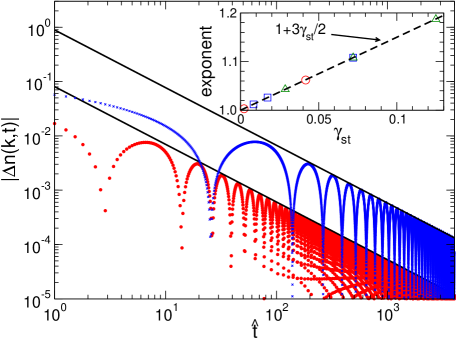
These analytical insights can be confirmed numerically by performing the integral in Eq. (55). Figure 1 shows $\left|\Delta n^{\rm adhoc}(k,t)\right|$ for fixed $\Delta\hat{k}=0.1$ (red circles) as well as $\Delta\hat{k}=0.01$ (blue crosses) and $\hat{v}=0.5$ on a double-logarithmic scale. The solid lines are power-law fits (for times $\hat{t}\in[400,4000]$) to the envelope. In the inset exponents extracted along this line for different $\hat{v}$ (and thus $\gamma_{\rm st}$; see Eq. (42)) and $\Delta\hat{k}$ are presented. They nicely fall onto the analytical prediction $1+\frac{3}{2}\gamma_{\rm st}$ shown as the dashed line. Consistent with the above analytical result the asymptotic behavior is reached faster the larger $\Delta\hat{k}$ (compare the data for $\Delta\hat{k}=0.1$ and $0.01$ in the main panel of Fig. 1).

4.1.3 The box potential

Analytical progress is also possible in the case of the box potential Eq. (32). Then the argument of the exponential function in Eq. (24) simplifies to

$$I = \int_{0}^{\infty}dk\,\frac{4s^{2}(k)c^{2}(k)}{k}\left(\cos{[kx]}-1\right)\left(1-\cos{\left[2\omega(k)t\right]}\right)$$ (57)

$$= \gamma_{\rm st}\int_{0}^{1}dk\,\frac{\cos{[kq_{\rm c}x]}-1}{k}\left(1-\cos{\left[2\hat{v}_{\rm F}k\hat{t}\right]}\right)\;.$$

For asymptotically large $\hat{t}$ the integral can be evaluated using integration by parts

$$\mbox{}I=\gamma_{\rm st}\int_{0}^{1}dk\,\frac{\cos{[kq_{\rm c}x]}-1}{k}-\frac{\gamma_{\rm st}}{2\hat{v}_{\rm F}\hat{t}}\left(\cos{[q_{\rm c}x]}-1\right)\sin{(2\hat{v}_{\rm F}\hat{t})}+{\mathcal{O}}(\hat{t}^{-2})\;.$$ (58)

From this it straightforwardly follows that

$$\Delta n^{\rm box}(k,t)\sim\frac{\sin\left(2\hat{v}_{\rm F}\hat{t}\right)}{\hat{t}}\;.$$ (59)

The two characteristic differences to the asymptotic dynamics of the ad hoc procedure Eq. (56) namely the (i) independence of the decay exponent from the interaction strength and the (ii) independence of the oscillation frequency from the momentum $k-k_{\rm F}$ at which the distribution function is evaluated can be traced back to the nonanalyticity of the box potential; the long-time dynamics is dominated by the position of the jump in the potential, that is the upper boundary of the momentum integral in $I$.

Figure 2: The time dependence of $|\Delta n(k,t)|$ for the box potential with $\hat{v}=2$ at fixed $\Delta\hat{k}=0.4$ (red circles). The solid line shows a power law $\sim\hat{t}^{-1}$ which fits the data for sufficiently large $\hat{t}\gtrapprox 200$. Inset: Fourier spectrum of the data from the main plot.

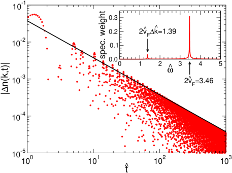
Figure 2 shows $\left|\Delta n^{\rm box}(k,t)\right|$ for fixed $\Delta\hat{k}=0.4$ and $\hat{v}=2$ obtained by numerically performing the momentum integral in Eq. (24) and the Fourier integral (with respect to position) Eq. (19). In the data a second smaller frequency than $2\hat{v}_{\rm F}$ is observable. A Fourier analysis (with respect to time) shows that it is equal to the frequency found for $\Delta n^{\rm adhoc}(k,t)$ and given by $2\hat{v}_{\rm F}\Delta\hat{k}$; see the inset of Fig. 2. In fact, the numerical data are consistent with the long-time dynamics for the box potential being dominated by the interplay of the term Eq. (59) and another one of the form Eq. (56). Considering a fixed time interval the $\hat{t}^{-1}$ decay is only clearly observable if the interaction and thus $\gamma_{\rm st}$ is not too small and the term Eq. (56) can be neglected compared to Eq. (59). Consistently, for such interactions the low-energy peak in the frequency spectrum carries a much lower weight than the high-energy one; see the inset of Fig. 2.

It is possible to provide analytical evidence for the appearance of the second term Eq. (56) at large $\hat{t}$. To this end one uses that the argument $I$ of the exponential function in Eq. (24) can be further evaluated

$$I = \gamma_{\rm st}\left[\mbox{Ci}(|q_{\rm c}x|)-\gamma-\ln(|q_{\rm c}x|)\right]+\gamma_{\rm st}\left[\mbox{Ci}(2\hat{v}_{\rm F}\hat{t})-\gamma-\ln(2\hat{v}_{\rm F}\hat{t})\right]$$ (60)

$$-\frac{\gamma_{\rm st}}{2}\left[\mbox{Ci}(|q_{\rm c}x+2\hat{v}_{\rm F}\hat{t}|)-\gamma-\ln(|q_{\rm c}x+2\hat{v}_{\rm F}\hat{t}|)\right]$$

$$-\frac{\gamma_{\rm st}}{2}\left[\mbox{Ci}(|q_{\rm c}x-2\hat{v}_{\rm F}\hat{t}|)-\gamma-\ln(|q_{\rm c}x-2\hat{v}_{\rm F}\hat{t}|)\right]$$

with the integral cosine function Ci and the Euler constant $\gamma$. With this $\left|\Delta n^{\rm box}(k,t)\right|$ can be brought into a form similar to Eq. (55)

$$\mbox{}\Delta n^{\rm box}(k,t) = -\frac{1}{\pi}\frac{\exp{(-\gamma\gamma_{\rm st})}}{(2\hat{v}_{\rm F}\hat{t})^{\gamma_{\rm st}}}\,\int_{0}^{\infty}dy\,\frac{\sin\left[2\hat{v}_{\rm F}\Delta\hat{k}\hat{t}y\right]}{y^{1+\gamma_{\rm st}}}\Big{[}(1+y)^{\gamma_{\rm st}/2}|1-y|^{\gamma_{\rm st}/2}$$ (61)

$$\times\exp{\left\{\gamma_{\rm st}\left[\mbox{Ci}(2\hat{v}_{\rm F}\hat{t})-\mbox{Ci}(2\hat{v}_{\rm F}\hat{t}[y+1])/2-\mbox{Ci}(2\hat{v}_{\rm F}\hat{t}|y-1|)/2\right]\right\}}-1\Big{]}.$$

Leaving out the sine factor and considering large $\hat{t}$ the integrand has similar to the one of Eq. (55) a cusp at $y=1$. This again leads to a nonanalytic term of the form Eq. (56). In fact, the integrands (as a function of $y$) of the box potential and the ad hoc procedure coincide close to $y=1$ up to the crucial difference that for the box potential the cusp-like behavior is modulated by an oscillation with frequency $2\hat{v}_{\rm F}\hat{t}$ (associated to the oscillatory behavior of Ci). Taking everything together the appearance of the two terms Eqs. (56) and (59) is thus plausible from the analytics.

To observe the power-law decay of $\left|\Delta n^{\rm box}(k,t)\right|$ for fixed $k-k_{\rm F}$ in a given time interval (at large times) one again has to stay away from the nonanalyticity (the jump for finite $t$) at $k=k_{\rm F}$: the smaller $\left|\Delta\hat{k}\right|$ the longer it takes before the asymptotic power-law behavior sets in.

4.1.4 Stationary points in $\omega(k)$

For the regular potentials Eqs. (33)-(35) the dispersion $\omega(k)$ Eq. (11) is a nonlinear function of the momentum. For each of the potentials a critical interaction strength $\hat{v}_{\rm c}$ exists beyond which $\omega(k)$ has two stationary points. For the Gaussian potential one e.g. finds $\hat{v}_{\rm c}=e^{2}\approx 7.39$. For $\hat{v}>\hat{v}_{\rm c}$ the large time dynamics of Eq. (24) is dominated by these stationary points. Using the stationary phase method [31] it is straightforward to show that on asymptotic time scales

$$\mbox{}\Delta n(k,t)\sim c_{1}\,\frac{\sin{[2\hat{\omega}(k_{1})\hat{t}+\phi_{1}]}}{\sqrt{\hat{t}}}+c_{2}\,\frac{\sin{[2\hat{\omega}(k_{2})\hat{t}+\phi_{2}]}}{\sqrt{\hat{t}}}\;,$$ (62)

with amplitudes $c_{1/2}$, phases $\phi_{1/2}$, the two stationary points $k_{1/2}$, and the dimensionless dispersion $\hat{\omega}(k)=\omega(k)/(v_{\rm F}q_{\rm c})$. Here we are primarily interested in the behavior at small to intermediate interactions (see also the above subsection on the ad hoc procedure) and thus focus on $\hat{v}<\hat{v}_{\rm c}$ from now on.

4.2 Numerical results

For the Gaussian Eq. (33), the exponential Eq. (34), and the quartic potential Eq. (35) we did not succeed in obtaining analytical results for $\Delta n(k,t)$. The following analysis thus solely relies on the numerical evaluation of the momentum integral in Eq. (24) and the successive Fourier integral Eq. (19). As the integrands are oscillatory functions one has to use routines which are adopted to this situation. Furthermore, for large times $|\Delta n(k,t)|$ becomes very small (of order $10^{-8}$ and smaller) which requires a very accurate evaluation of the integrals. This limits the numerics and reliable results can be obtained up to times of the order of $\hat{t}=5000$.

Figure 3: Exponents of the power-law decay of $|\Delta n(k,t)|$ for different potentials (symbols) as a function of $\gamma_{\rm st}$, that is the interaction strength (see Eq.(42)). The solid line shows $1+\gamma_{\rm st}$, the dashed one the exponent $1+3\gamma_{\rm st}/2$ obtained within the ad hoc procedure. (a) Fixed momentum $\Delta\hat{k}=0.8$ and (b) $\Delta\hat{k}=0.4$.

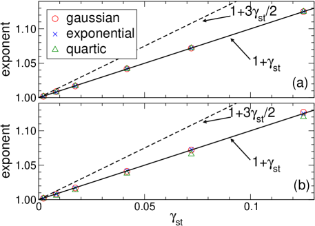
From the above analytical consideration we expect that (i) $|\Delta n(k,t)|$ decays as a power law in $\hat{t}$ and that (ii) this should be observable on moderately large times if $\left|\Delta\hat{k}\right|$ does not become too small. Our numerical results for $|\Delta n(k,t)|$ (not shown; the general form is similar to the data of Fig. 1) are consistent with this expectation. In Fig. 3 we show how exponents extracted by a power-law fit of $|\Delta n(k,t)|$ for times $\hat{t}\in[100,2400]$ depend on $\gamma_{\rm st}$, that is $\hat{v}$ (symbols). In Fig. 3(a) the momentum is fixed at $\Delta\hat{k}=0.8$ and in Fig. 3(b) at $\Delta\hat{k}=0.4$. The dashed line shows the result $1+3\gamma_{\rm st}/2$ obtained for the exponent within the ad hoc procedure. Obviously the data for the three potentials coincide and differ from $1+3\gamma_{\rm st}/2$ as well as the exponent 1 found for the box potential. In Fig. 3(a) they instead nicely fall onto the line $1+\gamma_{\rm st}$. For smaller $\Delta\hat{k}=0.4$ the data slightly scatter around this line but are still consistent with it. The largest deviations are observed for the quartic potential (see below). Already at this stage of the analysis we can conclude that both the ad hoc procedure as well as the box potential fail in producing the exponent obtained for the more generic (regular) potentials.

In Fig. 4(a) we collected the data for the decay exponent of $|\Delta n(k,t)|$ as a function of $\gamma_{\rm st}$ for the Gaussian potential from Figs. 3(a) and (b) and added another set obtained for $\Delta\hat{k}=0.1$ (open symbols). For small $\left|\Delta\hat{k}\right|$ the extracted exponents fall between the lines $1+3\gamma_{\rm st}/2$ and $1+\gamma_{\rm st}$ and one might be tempted to conclude that the exponent depends on $k-k_{\rm F}$. To further investigate this we studied the dependence of the extracted exponent on the time interval over which the power law was fitted. We increased the upper boundary $\hat{t}_{\rm u}$ at fixed lower boundary $\hat{t}_{\rm l}$. For the three regular potentials and all the $\Delta\hat{k}$ we studied we found that by increasing $\hat{t}_{\rm u}$ the exponent tends towards $1+\gamma_{\rm st}$. In Fig. 4(b) we show the $\hat{t}_{\rm u}$ dependence of the extracted exponent for the Gaussian potential with $\hat{v}=0.5$, corresponding to $\gamma_{\rm st}\approx 0.0417$, and the relativ momenta $\Delta\hat{k}=0.15$, $\Delta\hat{k}=0.3$, and $\Delta\hat{k}=0.4$. For increasing fitting range with lower boundary $\hat{t}_{\rm l}=200$ the exponent has a clear tendency towards $1+\gamma_{\rm st}$ and appears to saturate for times we can reach within our numerics. We conclude that our results for the regular potentials are consistent with the assumption of an asymptotic power-law exponent which is independently of $k-k_{\rm F}$ given by $1+\gamma_{\rm st}$ (as long as $|k-k_{\rm F}|\neq 0$).

Figure 4: Exponents of the power-law decay of $|\Delta n(k,t)|$. (a) The open symbols show the exponent as a function of $\gamma_{\rm st}$ for the Gaussian potential and the momenta as given in the legend. The filled light blue triangles are for the quartic potential with $\Delta\hat{k}=0.1$. The solid line shows $1+\gamma_{\rm st}$ the dashed one the exponent $1+3\gamma_{\rm st}/2$. (b) The filled symbols show the dependence of the exponent on the upper boundary of the time interval over which the power law was fitted. The lower boundary is $\hat{t}=200$. The data were obtained for the Gaussian potential with $\hat{v}=0.5$, corresponding to $\gamma_{\rm st}\approx 0.0417$ and $\Delta\hat{k}=0.15$, $0.3$ as well as $0.4$.

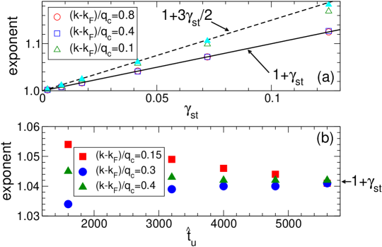
Figure 4(a) additionally contains data for the exponent of the quartic potential at $\Delta\hat{k}=0.1$ (filled light blue triangles) extracted for the time interval $\hat{t}\in[100,2400]$. The exponents are even closer to the result of the ad hoc procedure $1+3\gamma_{\rm st}/2$ than the corresponding ones for the Gaussian potential at the same $\Delta\hat{k}$ (open green triangles). This can be understood as follows. First one realizes that it is the momentum dependence of the dispersion $\omega(k)$ and not the one of the prefactor $s^{2}(k)c^{2}(k)$ in Eq. (24) which dominates the long-time dynamics of the Green function. In the ad hoc procedure the nonlinear dispersion $\omega(q)$ is replaced by the linear one $\tilde{v}_{\rm F}|q|$ (see Eq. (29)). For small momenta the quartic potential deviates from its zero momentum value only to fourth order in $q/q_{\rm c}$. This implies that for small $|q|/q_{c}$, $\omega(q)$ deviates from the linear behavior to fourth order and over the momentum range $0\leq|q|/q_{\rm c}\lessapprox 1$ the dispersion relation of the ad hoc procedure and the quartic potential coincide. This has to be contrasted to the deviation from a linear dispersion for the exponential and Gaussian potentials which is of first and second order in $q/q_{\rm c}$, respectively. In this sense the quartic potential is the one considered closest to the ad hoc procedure. For small $\left|\Delta\hat{k}\right|$ this implies, that an apparent power-law decay with exponent $1+3\gamma_{\rm st}/2$ is observable on intermediate times. Based on an analysis of the type discussed in the last paragraph we conclude that on asymptotic time scales the exponent will cross over to $1+\gamma_{\rm st}$.

Similar to the cases of the ad hoc procedure and the box potential also for the more regular potentials $\Delta n(k,t)$ oscillates around zero (with a decaying amplitude). A Fourier analysis (not shown) clearly reveals that the (dimensionless) frequency of the oscillation at fixed $k-k_{\rm F}$ is given by $2\hat{\omega}(k-k_{\rm F})$. This is consistent with the result for the ad hoc procedure for which $2\hat{\omega}(k-k_{\rm F})=2\hat{v}_{\rm F}|\Delta\hat{k}|$ because of the linearization.

A detailed account of the time dependence of $n(k,t)$ after a quench from one repulsive interaction to another one (obtained by Fourier transforming the Green function Eq. (25)) can be obtained along the same lines. This is left for future work.

5 Summary

We have studied the quench dynamics of the TL model focusing on the single-particle Green function and the fermionic momentum distribution function. Instead of using an ad hoc procedure to regularize momentum integrals in the ultraviolet we kept the momentum dependence of the two-particle interaction and considered different potentials. The steady-state momentum distribution function close to $k_{\rm F}$ is independently of the detailed form of the potential characterized by a power-law nonanalyticity with an exponent $\gamma_{\rm st}$ which depends via the LL parameter $K$ (or $K_{\rm i}$ and $K_{\rm f}$ when quenching between two repulsive interactions) on the strength of the interaction. We raised the question if this type of universality extends beyond the TL model to all models falling into the LL class in equilibrium. Importantly, $\gamma_{\rm st}$ differs from the exponent $\gamma_{\rm gs}$ characterizing the ground-state momentum distribution function at the same interaction. The ground-state and steady-state momentum distribution functions differ at weak coupling by a characteristic factor of two, known from systems in which pre-thermalized states appear.

Our analytical as well as numerical results for the asymptotic time dependence of $n(k,t)$ at small to intermediate interaction and $k-k_{\rm F}\neq 0$ are consistent with

$$\Delta n(k,t)\sim\frac{\sin{[\hat{\nu}(k)\hat{t}]}}{\hat{t}^{\xi}}\;.$$ (63)

For the class of generic regular potentials Eqs. (33)-(35) the frequency $\hat{\nu}(k)$ is given by $2\hat{\omega}(k-k_{\rm F})$ and the power-law exponent by $\xi=1+\gamma_{\rm st}$. While the frequency depends on the details of the potential (the nonlinearity of the dispersion) the exponent of this class of potentials turns out to be universal in the LL sense; it is solely determined by the potential at zero momentum transfer and thus the LL parameter $K$. Both, the nonanalytic box potential as well as the commonly employed ad hoc procedure fail in reproducing this universal behavior. For the box potential $\xi=1$ independent of the interaction strength and the (dimensionless) frequency is for all $\Delta\hat{k}$ given by $2\hat{v}_{\rm F}$. In the ad hoc procedure we obtain a larger decay exponent $\xi=1+3\gamma_{\rm st}/2$ and the frequency of the linearized dispersion $\hat{\nu}(k)=2\hat{v}_{\rm F}|\Delta\hat{k}|$. At $k=k_{\rm F}$, $n(k,t)$ has a Fermi liquid-like jump of height $Z(t)\sim\hat{t}^{-\gamma_{\rm st}}$. This holds independent of the potential considered. The time scale $\hat{t}_{\rm p}$ on which the power-law decay Eq. (63) is observable at fixed $k-k_{\rm F}$ increases if $k$ approaches $k_{\rm F}$. If $\hat{t}\gg\hat{t}_{\rm p}$ is not fulfilled the asymptotic behavior Eq. (63) might be superimposed or even hidden by additional contributions.

In analogy to the posed question of LL-like universality in the steady state it would again be very interesting to investigate if some form of universality in the time dependence extends beyond the TL model studying the quench dynamics of other models falling into the LL universality class in equilibrium. Two obvious candidates would be the decay exponent $1+\gamma_{\rm st}$ of $|\Delta n(k,t)|$ found for regular potentials in the TL model and the exponent $\gamma_{\rm st}$ of the jump at $k_{\rm F}$.

Studying the TL model with momentum dependent two-particle potentials we here performed the necessary first step towards a more detailed understanding of universality in the quench dynamics of LLs.

Acknowledgments: We are grateful to Jean-Sébastien Caux, Fabian Essler, Christoph Karrasch, Stefan Kehrein, Dante Kennes, Florian Marquardt, Kurt Schönhammer, and Nils Wentzell for fruitful discussions. This work was supported by the DFG via the Emmy-Noether program (D.S.) and FOR 912 (V.M.).

References

- [1] Bloch I, Dalibard J and Zwerger W 2008 Rev. Mod. Phys. 80 885
- [2] Polkovnikov A, Sengupta, K, Silva A and Vengalattore M 2011 Rev. Mod. Phys. 83 863
- [3] Voit J 1995 Rep. Prog. Phys. 58 977
- [4] Giamarchi T 2003 Quantum Physics in One Dimension (New York: Oxford University Press)
- [5] Schönhammer K 2005 in Interacting Electrons in Low Dimensions ed. by D. Baeriswyl (Dordrecht: Kluwer Academic Publishers)
- [6] Essler FHL, Frahm H, Göhmann F, Klümper A and Korepin VE 2005 The One-Dimensional Hubbard Model (Cambridge: Cambridge University Press)
- [7] Daley AJ, Kollath C, Schollwöck U and Vidal G 2004 J. Stat. Mech. (2004) P04005
- [8] Manmana SR, Wessel S, Noack RM and Muramatsu A 2007 Phys. Rev. Lett. 98 210405
- [9] Karrasch C, Bardarson JH and Moore JE 2011 arXiv:1111.4508v1
- [10] Calabrese P and Cardy J 2007 J. Stat. Mech. (2007) P06008
- [11] Kollar M and Eckstein M 2008 Phys. Rev. A 78 013626
- [12] Schiró M and Fabrizio M 2010 Phys. Rev. Lett. 105 076401
- [13] Mossel J, Palacios G and Caux J-S 2010 J. Stat. Mech. (2010) L09001
- [14] Gritsev V, Rostunov T and Demler E 2010 J. Stat. Mech. (2010) P05012
- [15] Calabrese P, Essler FHL and Fagotti M 2011 Phys. Rev. Lett. 106 227203
- [16] Goth F and Assaad F 2011 arXiv:11082703v1
- [17] Haldane FDM 1981 J. Phys. C 14 2585
- [18] Sólyom J 1979 Adv. Phys. 28 201
- [19] Cazalilla MA 2006 Phys. Rev. Lett. 97 156403
- [20] Perfetto E 2006 Phys. Rev. B 74 205123
- [21] Kennes DM and Meden V 2010 Phys. Rev. B 82 085109
- [22] Dóra B, Haque M and Zarańd G 2011 Phys. Rev. Lett. 106 156406
- [23] Mitra A and Giamarchi T 2011 Phys. Rev. Lett. 107 150602
- [24] Iucci A and Cazalilla MA 2009 Phys. Rev. A 80 063619
- [25] Meden V 1999 Phys. Rev. B 60 4571
- [26] Moeckel M and Kehrein S 2008 Phys. Rev. Lett. 100 175702
- [27] Moeckel M and Kehrein S 2009 Annals of Physics 324 2146
- [28] Kollar M, Wolf FA and Eckstein M 2011 Phys. Rev. B 84 054304
- [29] Mitra A and Giamarchi T 2012 arXiv:1110.3671v2
- [30] Luther A and Peschel I 1974 Phys. Rev. B 9 2911
- [31] Orszag SA and Bender CM 1999 Advanced Mathematical Methods for Scientists and Engineers (New York: Springer)
- [32] Imambekov A, Schmidt TL and Glazman LI 2011 arXiv:1110.1374v1
- [33] Rigol M, Dunjko V, Yurovsky V and Olshanii M 2007 Phys. Rev. Lett. 98 050405
- [34] Cramer M, Dawson CM, Eisert J and Osborne TJ 2008 Phys. Rev. Lett. 100 030602
- [35] Barthel T and Schollwöck U 2008 Phys. Rev. Lett. 100 100601