Autocalibration with the Minimum Number of Cameras
with Known Pixel Shape

Abstract

In 3D reconstruction, the recovery of the calibration parameters of the cameras is paramount since it provides metric information about the observed scene, e.g., measures of angles and ratios of distances. Autocalibration enables the estimation of the camera parameters without using a calibration device, but by enforcing simple constraints on the camera parameters. In the absence of information about the internal camera parameters such as the focal length and the principal point, the knowledge of the camera pixel shape is usually the only available constraint. Given a projective reconstruction of a rigid scene, we address the problem of the autocalibration of a minimal set of cameras with known pixel shape and otherwise arbitrarily varying intrinsic and extrinsic parameters. We propose an algorithm that only requires 5 cameras (the theoretical minimum), thus halving the number of cameras required by previous algorithms based on the same constraint. To this purpose, we introduce as our basic geometric tool the six-line conic variety (SLCV), consisting in the set of planes intersecting six given lines of 3D space in points of a conic. We show that the set of solutions of the Euclidean upgrading problem for three cameras with known pixel shape can be parameterized in a computationally efficient way. This parameterization is then used to solve autocalibration from five or more cameras, reducing the three-dimensional search space to a two-dimensional one. We provide experiments with real images showing the good performance of the technique.

1 Introduction

Three-dimensional reconstructions from images are often obtained with calibrated cameras, i.e., cameras whose parameters have been previously computed using calibration objects in a controlled environment (YiMaLibro, , p. 201). Unfortunately, in many cases such conditions are not available, e.g., when the images have been acquired with non-specialized equipment or taken with a different initial purpose. To obtain 3D reconstructions without knowledge of the scene content and with partial knowledge of the camera parameters, camera autocalibration algorithms are needed.

Camera autocalibration comprises a family of techniques that apply to different scenarios depending on the a priori information (i.e., constraints) of the internal camera parameters. In the first works on autocalibration Maybank-Faugeras ; Faugeras92TE , the assumption was that the internal camera parameters were unknown but constant. Later, other techniques were developed to deal with different assumptions on the focal length, the principal point, the skew or the aspect ratio (see (Hartley-Zisserman, , Ch. 19)). The more a priori information one can incorporate in an autocalibration method, the better the results are expected to be. Therefore, there is no decisive solution to autocalibration in all situations.

A common framework for autocalibration was provided by the concept of geometric stratification Luong1996 ; Faugeras95stratificationof . This technique splits the camera calibration and scene reconstruction into three steps: first, the recovery of a projective reconstruction, i.e., a 3D scene and a set of cameras differing from the actual ones in a spatial homography. Second, the obtainment of an affine reconstruction (differing from the actual 3D scene in an affine transformation) by finding the location of the plane at infinity Pollefeys . Finally, the upgrading to a Euclidean reconstruction (differing from the actual scene in a similarity) by localizing the absolute conic at infinity or any equivalent geometric object. General references for the subject are Hartley-Zisserman ; Faugeras-Luong , where an extensive bibliography can be found. A review of camera self-calibration techniques is also presented in SurveySelfCalib2003 .

In order to upgrade a projective reconstruction to an affine or a Euclidean one in the absence of knowledge about the scene, some data about the camera parameters must be available. For example, in the originally addressed autocalibration problem, this additional piece of data was the constancy of the camera intrinsic parameters Maybank-Faugeras ; Faugeras92TE , resulting, for each camera pair, in a couple of polynomial equations in the camera parameters known as Kruppa equations. The instability problems of these equations have been studied in Sturm00 . Another constraint that has been studied is that in which the principal point is assumed to be known. Then the dual absolute quadric Triggs97 , a geometric object which encapsulates the information of both the plane at infinity (needed for affine upgrading) and the absolute conic (required for Euclidean upgrading), can be found by solving a set of homogeneous linear equations Seo2000 .

In this paper we address the problem of autocalibration in its less restrictive setting in practice: cameras with arbitrarily varying parameters with the exception of the pixel shape, which is assumed to be known. This is an important scenario since the pixel shape is unaffected by changes in focus and zoom. It can be easily seen (see Sect. 2) that this constraint is equivalent to having cameras with square pixels. The possibility of employing this constraint was studied in HeydenAstrom , where an algorithm based on bundle adjustment Triggs99Bundle was considered. Algorithms based on this restriction have also been proposed Ponce2 ; Valdes04 ; Valdes06 that result in a set of linear equations, but with the drawback of requiring 10 or more cameras. These algorithms are inspired by the geometric observation that, from the optical center of each square-pixel camera, two lines can be identified in the projective reconstruction that must intersect the absolute conic. The absolute quadratic complex (AQC) encodes the set of lines intersecting this conic by means of a quadric in a higher dimensional space ($\mathbb{P}^{5}$), which is the natural space containing Plücker coordinates of lines. The AQC, being represented by a homogeneous symmetric $6\times 6$ matrix satisfying a linear constraint, depends linearly on $21-1-1=19$ non-homogeneous parameters, which explains the need for such a large number of 10 views.

However, an informal parameter count reveals that far fewer cameras are theoretically sufficient. In fact, our main unknown is a space homography, which depends on 15 parameters. Being our target reconstruction defined up to a similarity, which depends on 7 parameters, there are $15-7=8$ unknowns left to be found, which correspond to the degrees of freedom (dof) needed to determine the plane at infinity (3 dof) and the absolute conic within it (5 dof). Knowing camera skew and aspect ratio amounts to two equations per camera and thus at least 4 cameras should be given in order to solve the problem. Given the non-linear nature of these equations, multiple solutions can be expected and so 5 cameras should be the minimum required to obtain, generically, a unique solution (see (Hartley-Zisserman, , Table 19.3), Pollefeys99b ).

The main contribution of this paper is a technique to obtain a Euclidean reconstruction for an arbitrary number of cameras equal or above the theoretical minimum, which is 5, using exclusively the pixel shape restriction. The basic geometric idea of this paper consists in the characterization of the candidate planes at infinity as those that intersect the isotropic lines of the cameras in points of a conic. In fact, this geometric approach was already pointed out in the late 19th century Finsterwalder ; Sturm11 . Finsterwalder showed that from multiple images of a rigid scene, projective reconstruction is possible. He showed that for unknown focal lengths and principal points, one may back-project all image cyclic points to 3D and find the plane at infinity as the one which cuts all those 3D lines in points which lie on a single conic. He also explains that 4 cameras should be the minimal case but that multiple solutions will exist. However, no algorithm was provided. In this paper, we provide such an algorithm. The geometric object that will be employed for this purpose is the variety of conics intersecting six given spatial lines simultaneously, which will be termed the six-lines conic variety (SLCV). The SLCV as a geometrical entity has been studied in schroecker , although our treatment is independent and self-contained. In this paper we are interested in the SLCV given by the absolute conic at infinity.

Table 1: Comparison of the Absolute Quadratic Complex (AQC) and the Six-Line Conic Variety (SLCV) approaches.

	AQC	SLCV
Common features
Basic geometric object	Isotropic lines through the optical centers of the cameras.
Intrinsic parameter assumption	Known pixel shape (skew and aspect ratio).
Differences
Type of algorithm	Linear (solution of a	Non-linear (bidimensional search
	homogeneous system).	using second degree equations).
Required number of cameras	$\geq 10$	$\geq 5$
Optimal w.r.t. number of cameras	No	Yes
Geometric object used	Quadric of $\mathbb{P}^{5}$	Algebraic surface of $\mathbb{P}^{3\ast}$ (set of planes of 3-space)
Degree of the geometric object	2	5
Geometric meaning	Lines intersecting the absolute conic.	Planes with conics intersecting all the isotropic lines.
Integration with scene knowledge	Pairs of orthogonal lines.	Parallel lines. Points at infinity.

The SLCV for six lines in generic position can be identified with a surface of $\mathbb{P}^{3*}$ (i.e., the projective space given by the planes of 3D space) of degree 8. We prove that this degree reduces to 5 in the case of the three pairs of isotropic lines of three finite square-pixel cameras. We show that the fifth-degree SLCV  has three singularities of multiplicity three, given by the three principal planes of the cameras. This result is used in Algorithm 1 to generate a bidimensional parameterization of the candidate planes at infinity compatible with three square-pixel cameras. This parameterization, together with the additional data given by another two or more square-pixel cameras permits to identify the true plane at infinity through a two-dimensional optimization process, leading to Algorithm 2. However, the technique could as well use other additional data such as some scene constraints. Table 1 summarizes the similarities and differences between the SLCV and the AQC and the algorithms built upon them.

Experiments with real images for the autocalibration of scenes with 5 or more cameras with square pixels and otherwise varying parameters are provided, showing the good performance of the proposed technique compared to other autocalibration methods. In the absence of knowledge about the principal point of the cameras, the SLCV algorithm turns out to be a feasible approach to solve the autocalibration problem, not requiring a previous initialization with an approximate solution, in the minimal case of 5 cameras up to the case of 9 cameras. For 10 or more cameras, the results are similar to those of the AQC algorithm.

The paper is organized as follows: The basic background for the problem is briefly recalled in Sect. 2. Section 3 presents the SLCV along with the basic algebraic geometry tools required for its definition and analysis as well as our main theoretical results. The algorithms motivated by these results are presented in Sect. 4 and the corresponding experiments are shown in Sect 5. A comparison with other search-based autocalibration algorithms is discussed in Sect. 6. Conclusions of the paper are found in Sect. 7. An advance of some of the results of this paper appeared in the conference paper Carballeira .

2 Camera model and preliminary problem analysis

We suppose that the cameras can be described using the pinhole camera model Hartley-Zisserman , which is defined by the optical center $\mathbf{C}$ and the projection plane endowed with an affine coordinate system given by the pixel structure of the camera.

The equations of the projection are linear when expressed in homogeneous coordinates, which are defined as follows. Any non-zero vector $(U,V,W)^{\top}$ proportional to $(u,v,1)^{\top}$ are the homogeneous coordinates of the point with usual coordinates $(u,v)^{\top}$. The set of all 3-vectors, considering them equal if they are proportional, is the projective space $\mathbb{P}^{2}$. If we suppose the coordinates are Euclidean, the elements of $\mathbb{P}^{2}$ with non-zero last coordinate constitute homogeneous coordinates of points of the plane, whereas those elements with vanishing last coordinate are identified with points at infinity in a Euclidean reference. The definition extends in a straightforward manner to spaces of arbitrary dimensions.

The equations of the projection are of the form $\mathbf{x}\sim\mathtt{P}\mathbf{X}$ where  the  symbol $\sim$ represents  vector  proportionality, $\mathtt{P}=\mathtt{K}(\mathtt{R}\,|\,-\mathtt{R}\widetilde{\mathbf{C}})$ is the projection matrix of the camera, $\mathbf{X}=(X,Y,Z,T)^{\top}$ are the homogeneous Euclidean coordinates of a 3D point, $\mathbf{x}=(x,y,z)^{\top}$ are the homogeneous coordinates of its projection, $\mathtt{R}$ is a rotation matrix, $\widetilde{\mathbf{C}}$ are the usual Euclidean coordinates of the optical center, and $\mathtt{K}$ is the intrinsic parameter matrix, given by

$$\mathtt{K}=\begin{pmatrix}fm_{x}&-fm_{x}\cot\theta&u_{0}\\ 0&fm_{y}/\sin\theta&v_{0}\\ 0&0&1\end{pmatrix},$$

where $f$ is the focal length, $m_{x}$ and $m_{y}$ are the number of pixels per distance unit in image coordinates in the $x$ and $y$ directions, $\theta$ is the skew angle and $(u_{0},v_{0})$ is the principal point.

If the camera aspect ratio $\tau=m_{y}/m_{x}$ and the skew angle $\theta$ are known, the affine coordinate transformation given in homogeneous coordinates by matrix

$$\mathtt{A}=\begin{pmatrix}\tau&\cos\theta&0\\ 0&\sin\theta&0\\ 0&0&1\end{pmatrix}$$

of the image plane permits to assume that the intrinsic parameter matrix has the form

$$\mathtt{K}=\begin{pmatrix}\alpha&0&u^{\prime}_{0}\\ 0&\alpha&v^{\prime}_{0}\\ 0&0&1\end{pmatrix},$$ (1)

which is the intrinsic parameter matrix of a square-pixel camera, i.e., one for which $\tau=1$ and $\theta=\pi/2$.

The back-projected lines of cyclic points at infinity ${\bf I}=(1,i,0)^{\top}$ and $\bar{{\bf I}}=(1,-i,0)^{\top}$ are the isotropic lines of the camera. These lines intersect the absolute conic, for if $\mathbf{X}=(X,Y,Z,0)^{\top}$ is the intersection of one of these two lines with the plane at infinity, we have

$$(1,\pm i,0)^{\top}\sim\mathtt{P}\mathbf{X}=\mathtt{K}\mathtt{R}(X,Y,Z)^{\top},$$

so that

$$(X,Y,Z)^{\top}\sim\mathtt{R}^{\top}\mathtt{K}^{-1}(1,\pm i,0)^{\top},$$

and then

$$X^{2}+Y^{2}+Z^{2} =(X,Y,Z)(X,Y,Z)^{\top}$$

$$=(1,\pm i,0)\mathtt{K}^{-\top}\mathtt{R}\mathtt{R}^{\top}\mathtt{K}^{-1}(1,\pm i,0)^{\top}$$

$$=\begin{pmatrix}1&\pm i\end{pmatrix}\begin{pmatrix}\alpha^{-2}&0\\ 0&\alpha^{-2}\end{pmatrix}\begin{pmatrix}1\\ \pm i\end{pmatrix}=0.$$

This equation can be expressed as

$$\mathbf{I}^{\top}\omega\mathbf{I}=0,\qquad\bar{\mathbf{I}}^{\top}\omega\bar{\mathbf{I}}=0,$$ (2)

which is the square-pixel condition in terms of the image of the absolute conic (IAC) $\boldsymbol{\omega}=(\mathtt{K}\mathtt{K}^{\top})^{-1}$.

We recall here that it is possible to obtain a projective calibration from image point correspondences only in uncalibrated images. This means that, given a sufficient number of projected points $\mathbf{x}_{ij}$ obtained with $N_{c}\geq 2$ cameras, we can obtain a set of matrices $\hat{\mathtt{P}}_{i}$ and a set of point coordinates $\hat{\mathbf{X}}_{j}$ such that $\mathbf{x}_{ij}\sim\hat{\mathtt{P}}_{i}\hat{\mathbf{X}}_{j}$, where $\hat{\mathtt{P}}_{i}=\mathtt{P}_{i}\mathtt{H}^{-1}$ and $\hat{\mathbf{X}}_{j}=\mathtt{H}\mathbf{X}_{j}$ for some non-singular $4\times 4$ matrix $\mathtt{H}$. Projective reconstruction from feature correspondences is a mature topic in computer vision. It was mostly developed during the 90’s stemming from the extension of the stereo reconstruction method of Longuet-Higgins LonguetHiggins to the case of uncalibrated images Faugeras ; HartleyCVPR92 (two views), QuanTrifocal94 ; Hartley94Invariants (three views), Mohr93cvpr ; Triggs95thegeometry (multiple views), etc. Nowadays there are excellent reference books collecting the contributions of many researchers in this field; see, for example Hartley-Zisserman ; Faugeras-Luong ; YiMaLibro .

Euclidean calibration can be defined as the obtainment of a matrix $\mathtt{H}$ changing the projective coordinates of a given projective calibration to some Euclidean coordinate system. It is well-known that Euclidean calibration up to a scale factor is equivalent to the recovery of the absolute conic at infinity $\Omega_{\infty}$ (see (Hartley-Zisserman, , p. 272), (Faugeras-Luong, , §1.18)), or any equivalent object such as the dual absolute quadric (DAQ) Triggs97 . To motivate our approach, let us check the possibility of addressing this autocalibration problem using the DAQ. The DAQ is given by the planes tangent to the absolute conic and it is algebraically defined as a rank-three projective mapping $\mathtt{Q}^{\ast}_{\infty}:\mathbb{P}^{3\ast}\to\mathbb{P}^{3}$. Its matrix it is related to the matrix of the dual IAC (DIAC) by

$$\omega^{\ast}\sim\mathtt{P}\mathtt{Q}^{\ast}_{\infty}\mathtt{P}^{\top},$$ (3)

where $\mathtt{P}$ is the matrix of the considered projective camera. If the camera has square pixels, it is known that the matrix of the DIAC is of the form

$$\omega^{\ast}\sim\begin{pmatrix}\alpha^{2}+x_{0}^{2}&x_{0}y_{0}&x_{0}\\ x_{0}y_{0}&\alpha^{2}+y_{0}^{2}&y_{0}\\ x_{0}&y_{0}&1\end{pmatrix}.$$

This leads to the equations

$$\begin{split}\omega^{\ast}_{12}\omega^{\ast}_{33}-\omega^{\ast}_{13}\omega^{\ast}_{23}&=0\\ \omega^{\ast}_{33}\omega^{\ast}_{11}-\left(\omega^{\ast}_{13}\right)^{2}&=\omega^{\ast}_{33}\omega^{\ast}_{22}-\left(\omega^{\ast}_{23}\right)^{2}.\end{split}$$ (4)

Using relation (3), Eqs. (4) turn out to be two quadratic equations in the coefficients of $\mathtt{Q}^{\ast}_{\infty}$ obtained for each camera $\mathtt{P}$. The DAQ $\mathtt{Q}^{\ast}_{\infty}$ is homogeneous and symmetric, so it is described by $9$ parameters. Therefore four cameras will lead to $8$ quadratic equations which, together with the quartic constraint $\det\mathtt{Q}^{\ast}_{\infty}=0$ would determine a discrete number of possible solutions. One more camera would allow to decide which of these solutions is the correct one.

Given the large number of variables and the nonlinear nature of the equations, this approach does not seem very promising from a practical point of view. As we will see, the alternative we propose in this paper reduces the problem to a 5th-degree equations in three variables, which allows a two dimensional parameterization of the possible planes at infinity from which we will be able to do an efficient search of those compatible with the intrinsic geometry of the cameras.

3 The six line conic variety

Let us suppose we have a projective calibration of three square-pixel cameras (or, as explained before, cameras with known pixel shape) and let $\mathtt{P}_{i}$ be their camera matrices and $\text{$\mathbf{C}$}_{i}$ their optical centers, $i=1,2,3$. Let us denote by $l_{i},\bar{l}_{i}$ the isotropic lines of camera $i$. The plane at infinity $\boldsymbol{\pi}_{\infty}$ will intersect these lines in points of the absolute conic. Therefore the planes $\pi$ candidates to be the plane at infinity are those intersecting the isotropic lines in points of a conic (see Fig. 1). We are going to see that these planes are given by a 5th-degree algebraic equation in their coordinates, $\boldsymbol{\pi}=(u_{1},u_{2},u_{3},u_{4})^{\top}$. To obtain this equation, some mathematical preliminaries are needed.

Figure 1: Illustration of the incidence relations between the isotropic lines of three cameras, the plane at infinity and the absolute conic.

3.1 The equation of the six-line conic variety

We recall, see e.g. (Hartley-Zisserman, , p. 70), that lines of 3-space are in one-to-one correspondence with non-null singular antisymmetric $4\times 4$ matrices (or, equivalently, non-null rank-2 antisymmetric matrices, since antisymmetric matrices have even rank) defined up to a non-zero scalar factor. The correspondence is given by the mapping that assigns to the line $l$ passing through points $\mathbf{p},\mathbf{q}$ the Plücker matrix $\mathtt{L}=\mathtt{M}(\mathbf{p},\mathbf{q})=\mathbf{p}\mathbf{q}^{\top}-\mathbf{q}\mathbf{p}^{\top}$. There is an equivalent mapping attaching to the line determined by planes $\boldsymbol{\alpha},\boldsymbol{\beta}$ the matrix $\mathtt{L}^{*}=\mathtt{M}(\boldsymbol{\alpha},\boldsymbol{\beta})$. These two matrices are related by the transformation $*:\mathtt{L}=(m_{ij})\mapsto\mathtt{L}^{*}$ where

$$\mathtt{L}^{*}=\begin{pmatrix}0&m_{34}&m_{42}&m_{23}\\ -m_{34}&0&m_{14}&m_{31}\\ -m_{42}&-m_{14}&0&m_{12}\\ -m_{23}&-m_{31}&-m_{12}&0\end{pmatrix}.$$

We also recall that the intersection of the line of Plücker matrix $\mathtt{L}$ with the plane $\boldsymbol{\pi}=(u_{1},u_{2},u_{3},u_{4})^{\top}$ is the point $\mathbf{p}=\mathtt{L}\boldsymbol{\pi}$, which is zero if and only if the line $\mathtt{L}$ is contained in $\boldsymbol{\pi}$.

If $\mathtt{H}$ is a coordinate change $\mathbf{X}^{\prime}=\mathtt{H}\mathbf{X}$, the line $\mathtt{L}$ is written in the new coordinate system as

$$\mathtt{L}^{\prime}=\mathtt{H}\mathtt{L}\mathtt{H}^{\top}.$$ (5)

The degree-two Veronese mapping $\nu_{2}$ maps a point $\mathbf{x}$ to the pairwise product of its coordinates. In particular, for $n=2,3$ we define:

$$\begin{split}\nu_{2}(x_{1},x_{2},x_{3})^{\top}&=(x_{1}^{2},x_{1}x_{2},x_{1}x_{3},x_{2}^{2},x_{2}x_{3},x_{3}^{2})^{\top},\\ \nu_{2}(x_{1},x_{2},x_{3},x_{4})^{\top}&=(x_{1}^{2},x_{1}x_{2},x_{1}x_{3},x_{1}x_{4},x_{2}^{2},\\ &\qquad x_{2}x_{3},x_{2}x_{4},x_{3}^{2},x_{3}x_{4},x_{4}^{2})^{\top}.\end{split}$$

Observe that a point $\mathbf{x}$ in $\mathbb{P}^{2}$ belongs to the conic of matrix $\mathtt{C}=(c_{ij})$ if and only if $\mathbf{x}^{\top}\mathtt{C}\,\mathbf{x}=0$, which in terms of $\nu_{2}$ can be written as

$$\nu_{2}(\mathbf{x})^{\top}\bar{\mathtt{C}}=0,\quad\text{where}\quad\bar{\mathtt{C}}=\Bigl{(}c_{11},\frac{c_{12}}{2},\frac{c_{13}}{2},c_{22},\frac{c_{23}}{2},c_{33}\Bigr{)}^{\top}.$$

Hence, six points $\mathbf{q}_{1},\ldots,\mathbf{q}_{6}$ of the plane lie on a conic if and only if for some non-zero vector $\bar{\mathtt{C}}$

$$\left(\nu_{2}(\mathbf{q}_{1})\cdots\nu_{2}(\mathbf{q}_{6})\right)^{\top}\bar{\mathtt{C}}=0,$$ (6)

which is equivalent to the singularity of the matrix, i.e.,

$$\det\left(\nu_{2}(\mathbf{q}_{1})\cdots\nu_{2}(\mathbf{q}_{6})\right)=0.$$

Similarly, $10$ points $\mathbf{q}_{i}$ of 3-space lie on a quadric if and only if

$$\det\left(\nu_{2}(\mathbf{q}_{1}),\ldots,\nu_{2}(\mathbf{q}_{10})\right)=0.$$

Next, using the previous results for lines and conics, we characterize whether the intersection of lines with a plane is contained in points of a conic.

Result 1

Given six lines with Plücker matrices $\mathtt{L}_{i}$ and vectors $\boldsymbol{\pi},\mathbf{a}_{1},\ldots,\mathbf{a}_{4}$ in $\mathbb{C}^{4}$, let us consider the polynomial

$$\begin{split}&D(\boldsymbol{\pi},\mathbf{a}_{1},\ldots,\mathbf{a}_{4})=\\ &\quad\det\left(\nu_{2}(\mathtt{L}_{1}\boldsymbol{\pi}),\ldots,\nu_{2}(\mathtt{L}_{6}\boldsymbol{\pi}),\nu_{2}(\mathbf{a}_{1}),\ldots,\nu_{2}(\mathbf{a}_{4})\right).\end{split}$$ (7)

The set of planes $\boldsymbol{\pi}$ intersecting the six lines in points of a conic is defined by

$$D(\boldsymbol{\pi},\mathbf{a}_{1},\ldots,\mathbf{a}_{4})=0\;\;\text{ for all }\;\mathbf{a}_{1},\ldots,\mathbf{a}_{4}\text{ in }\mathbb{C}^{4}.$$

The proof of this result is given in Appendix A.

Being each column $\nu_{2}(\mathtt{L}_{i}\pi)$ of degree two in $\boldsymbol{\pi}$, the equation $D(\boldsymbol{\pi},\mathbf{a}_{1},\ldots,\mathbf{a}_{4})=0$ is of degree $12$ in the coordinates of the plane. Next result, proven in Appendix B, shows that we can factor out four trivial linear factors and obtain an 8th-degree polynomial in $\boldsymbol{\pi}$ which is also shown to be independent of the $\mathbf{a}_{j}$.

Result 2

The set of planes $\boldsymbol{\pi}$ intersecting the six lines with Plücker matrices $\mathtt{L}_{i}$ in points of a conic is given by the 8th-degree polynomial equation

$$F(\boldsymbol{\pi})=0$$ (8)

defined by the relationship

$$\begin{split}&D(\boldsymbol{\pi},\mathbf{a}_{1},\ldots,\mathbf{a}_{4})=\\ &\quad\det(\mathbf{a}_{1},\ldots,\mathbf{a}_{4})\,(\boldsymbol{\pi}^{\top}\mathbf{a}_{1})\cdots(\boldsymbol{\pi}^{\top}\mathbf{a}_{4})\,F(\boldsymbol{\pi}),\end{split}$$ (9)

Furthermore, the polynomial $F$ does not depend on the variables $\mathbf{a}_{j}$.

The surface of $\mathbb{P}^{3*}$ (set of planes of 3D space) given by the planes intersecting the six lines in points of a conic will be called the six-line conic variety (SLCV).

3.2 The SLCV given by the isotropic lines of three finite square-pixel cameras

In the particular case of three finite square-pixel cameras (i.e., cameras such that the optical center is a finite point), the configuration of the isotropic lines, which intersect pairwise in the optical centers $\mathbf{C}_{i}$, allows to further simplify the factorization from Result 2.

Result 3

Let us consider six lines with Plücker matrices $\mathtt{L}_{i}$ such that the pairs $\{\mathtt{L}_{1},\mathtt{L}_{2}\}$, $\{\mathtt{L}_{3},\mathtt{L}_{4}\}$ and $\{\mathtt{L}_{5},\mathtt{L}_{6}\}$ are intersecting in points $\mathbf{C}_{1},\mathbf{C}_{2}$ and $\mathbf{C}_{3}$, respectively. Then the set of planes $\boldsymbol{\pi}$ intersecting the six lines in points of a conic and not passing through any of the intersections $\mathbf{C}_{i}$ are real zeros of a 5th-degree polynomial $G$ defined by:

$$F(\boldsymbol{\pi})=(\boldsymbol{\pi}^{\top}\mathbf{C}_{1})(\boldsymbol{\pi}^{\top}\mathbf{C}_{2})(\boldsymbol{\pi}^{\top}\mathbf{C}_{3})\,G(\boldsymbol{\pi}).$$ (10)

Proof

We have proved in Result 2 that the set of planes intersecting the lines $\mathtt{L}_{i}$ in points of a conic is given by the zeroes of an 8th-degree polynomial, $F(\boldsymbol{\pi})$. Since the lines intersect by pairs at the points $\mathbf{C}_{i}$, there are trivial solutions of the equation $F(\boldsymbol{\pi})=0$, namely those corresponding to planes passing through any of the points $\mathbf{C}_{i}$. In fact, any plane through any of the $\mathbf{C}_{i}$ intersects the six lines in at most five different points. Since five points always lie on a conic, all planes through any of the $\mathbf{C}_{i}$ are zeros of $F$. Therefore, we can further factorize the polynomial $F$ as in equation (10). The planes intersecting the lines in points of a conic and not passing through the points $\mathbf{C}_{i}$ are solutions of (8) and, since $\boldsymbol{\pi}^{\top}\mathbf{C}_{i}\not=0$, they must be solutions of $G(\boldsymbol{\pi})=0$. ∎

Corollary 1

Given a projective reconstruction for three finite cameras, the planes at infinity compatible with the square-pixel property of the cameras are real zeros of a $5$th-degree polynomial $G$ given by:

$$F(\boldsymbol{\pi})=(\boldsymbol{\pi}^{\top}\mathbf{C}_{1})(\boldsymbol{\pi}^{\top}\mathbf{C}_{2})(\boldsymbol{\pi}^{\top}\mathbf{C}_{3})\,G(\boldsymbol{\pi}).$$ (11)

Proof

It is an immediate consequence of the previous result and the fact that the isotropic lines intersect by pairs in the optical centers of the cameras.∎

In the context of camera autocalibration, we will also use the term SLCV for the 5th-degree variety, from which the three trivial linear factors have been removed.

A straightforward application of this result is the direct obtainment of the candidate planes at infinity, when two points at infinity are known, as the real solutions of a fifth-degree polynomial equation in one variable (see Carballeira ).

Corollary 2

If two points of the plane at infinity are known, there are at most five candidate planes at infinity which can be found solving the 5th-degree equation in the homogeneous coordinates $\lambda:\mu$

$$G(\lambda\boldsymbol{\alpha}+\mu\boldsymbol{\beta})=0,$$

where $\boldsymbol{\alpha}$ and $\boldsymbol{\beta}$ are any two planes intersecting in the line determined by the two points at infinity.

3.3 Singularity of the principal planes

From now on, we suppose as above that the six lines are the isotropic lines of three square-pixel cameras. The following result is the key to find a computationally efficient way to parameterize the set of associated candidate planes. For our configuration of three cameras, we will say that a principal plane is generic if it does not contain the projection centers of any of the other two cameras.

We recall that a line intersects a complex projective hypersurface (or variety) of degree $d$ in $d$ points, counted with their multiplicity. A point $\mathbf{p}$ of the hypersurface $F(\mathbf{x})=0$ is a singular (multiple) point of multiplicity $r$ if $\lambda=0$ is an $r$-th order root of the equation $F(\mathbf{p}+\lambda\mathbf{q})=0$, for any $\mathbf{q}$ not in the hypersurface. Therefore, the line $\mathbf{p}\mathbf{q}$ intersects the variety in at most $d-r$ additional points. Singular points are useful to obtain parametrizations of the variety by computing its intersections with the lines through the point. For instance, given a 5-th degree variety with a point $\mathbf{p}$ of multiplicity 3, for each line through $\mathbf{p}$ there are at most two additional points of intersection of the line with the variety. The approach of using a triple point to parametrize a 5-th degree variety is illustrated in Fig. 2 for the case of a 2D curve.

Figure 2: Illustration of the approach to obtain the points of the SLCV.
The projective plane curve $G(\mathbf{p})=0$ is of degree five and has $\mathbf{p}_{0}$ as a triple point. Therefore, substituting in this equation the parametric equation of a line through this point, results in an equation of the form $G(\lambda\mathbf{p}_{0}+\mu\mathbf{q}_{0})=\mu^{3}H(\lambda,\mu)$, so that the other two points of intersection of the line and the curve are obtained by solving the quadratic equation $H(\lambda,\mu)=0$.

Result 4 below provides us with three very useful multiple planes in the SLCV (points, if we interpret the SLCV as a surface in the space of planes, $\mathbb{P}^{3*}$).

Result 4

Any generic principal plane is a singularity of multiplicity three of the variety of candidate planes $G(\boldsymbol{\pi})=0$.

Observe that, by point-plane duality, the lines through a point $\boldsymbol{\pi}$ of $\mathbb{P}^{3*}$ correspond in $\mathbb{P}^{3}$ to pencils of planes, i.e., sets of planes through a given line (its base) or, equivalently, linear combinations of two given planes. Result 4, proven in Appendix C, suggests to parameterize the set of candidate planes considering the pencils of planes with base contained in one of the principal planes. We will denote by $\boldsymbol{\pi}_{i}$, $i=1,2,3$ the principal planes of the cameras. Let us assume that $\boldsymbol{\pi}_{1}$ is a generic principal plane. To each pencil of planes that includes $\boldsymbol{\pi}_{1}$ we will associate two candidate planes. To parameterize the pencil, we can consider its element $\boldsymbol{\xi}$ through $\mathbf{C}_{2}$, so the pencil is given by the planes of the form $\lambda\boldsymbol{\pi}_{1}+\mu\boldsymbol{\xi}$ (see Fig. 3).

Figure 3: Elements in the parameterization of the SLCV given by Result 4.

Result 4 guarantees that the quintic polynomial $G(\lambda\boldsymbol{\pi}_{1}+\mu\boldsymbol{\xi})$ factorizes as

$$G(\lambda{\boldsymbol{\pi}_{1}}+\mu\boldsymbol{\xi})=\mu^{3}H(\lambda,\mu)$$ (12)

where $H$ is a homogeneous polynomial of degree $2$ whose zeroes provide the two candidate planes associated to $\boldsymbol{\xi}$.

Remark 1

Observe that only one generic principal plane is required in order to parametrize the set of solutions in the proposed way. The non-existence of generic principal planes constitutes a highly singular case, in which each optical center lies in the intersection of its principal plane with one of the other two. Result 4 can be easily extended to show that a non-generic principal plane containing exactly two optical centers is a singularity of multiplicity two. Therefore, using such a plane to parametrize the set of candidate planes $G(\boldsymbol{\pi})=0$ implies the solution of a polynomial equation of degree three for each line in the plane.

Finally, the following result can be useful as will be discussed in Sect. 6.

Result 5

The pencils of planes determined by any pair of principal planes is contained in the variety of candidate planes.

Proof

It is enough to observe that the base of such a pencil intersect the corresponding isotropic lines in four points and any six points, four of which are aligned, lie on a conic.

4 Algorithms

We have seen that the set of planes at infinity compatible with three cameras with square pixels is a surface given by a fifth-degree equation

$$G(\boldsymbol{\pi})=0.$$

This will allow to compute the plane at infinity by means of a two-dimensional search if enough additional data about the cameras or the scene are available. In the first part of this section we will address a convenient way to parameterize the surface of candidate planes, while in the second part we will focus on the particular case in which the additional information stems from the presence of two or more auxiliary square-pixel cameras.

4.1 Parameterization of the candidate planes

Exploiting Result 4 and assuming that the first principal plane $\boldsymbol{\pi}_{1}$ is generic, our algorithm will sweep the set of candidate planes at infinity corresponding to three square-pixel cameras. We will define a one-to-two mapping attaching to each real line $l$ of $\boldsymbol{\pi}_{1}$ the two candidate planes $\boldsymbol{\chi}_{1}$, $\boldsymbol{\chi}_{2}$ containing $l$, i.e., the intersection of the pencil of planes through $l$ with the variety of candidate planes. Hence, if we parameterize the set of real lines $l$ of $\boldsymbol{\pi}_{1}$ that do not contain the optical center $\mathbf{C}_{1}$, we will obtain accordingly a two-fold parameterization of the set of candidate planes. To this purpose we fix a point $\mathbf{r}$ in $l_{1}$ which, together with the optical center $\mathbf{C}_{1}$ will parameterize the points $\mathbf{q}$ in $l_{1}$ as $\mathbf{q}=\mathbf{r}+z\mathbf{C}_{1}$, $z$ being a complex number. We now define $l$ as the line through $\mathbf{q}$ and $\bar{\mathbf{q}}$ (see Fig. 4).

Figure 4: Geometric elements used in Algorithm 1. The three square-pixel cameras are represented by their optical centers $\mathbf{C}_{j}$ and their isotropic lines $l_{j},\bar{l}_{j}$ contained in the principal planes $\boldsymbol{\pi}_{j}$, $j=1,2,3$. Planes $\boldsymbol{\pi}_{1}$ and $\boldsymbol{\xi}$ are generators of the pencil of planes through the line joining $\mathbf{q}(z)$ and $\bar{\mathbf{q}}(z)$. Within the pencil, solution planes $\boldsymbol{\chi}_{i}(z)$, $i=1,2$ intersect the six isotropic lines in points of a conic.

We will consider as generators of the pencil of planes through $l$ the principal plane $\boldsymbol{\pi}_{1}$ and a plane $\boldsymbol{\xi}$ passing through $l$ and $\mathbf{C}_{2}$, so the planes of the pencil are of the form

$$\boldsymbol{\chi}=\lambda\boldsymbol{\pi}_{1}+\mu\boldsymbol{\xi}.$$

As explained in the previous section, the solutions contained in the pencil through $l$ will be the zeroes of the polynomial $H(\lambda,\mu)$ defined in (12). Since it is a homogeneous degree two polynomial, it has an expression of the form

$$H(\lambda,\mu)=A\lambda^{2}+B\lambda\mu+C\mu^{2},$$ (13)

where $A,B,C$ are polynomials in the coefficients of the Plücker matrices $\mathtt{L}_{i},\bar{\mathtt{L}}_{i}$ of the isotropic lines of the cameras. Their size, of the order of thousands of terms, is not suitable for algorithmic use. However, a convenient coordinate change shortens them so that they add up to about one hundred terms.

Specifically, denoting by $\mathbf{q}$ and $\bar{\mathbf{q}}$ the intersection points of the isotropic lines $l_{1}$ and $\bar{l}_{1}$ with the plane $\boldsymbol{\xi}$ and assuming that the points $\mathbf{C}_{i}$, $\mathbf{q}$ and $\bar{\mathbf{q}}$ are in general position, we consider the coordinate change $\mathtt{H}$ performing the mapping

$$\begin{split}\mathbf{C}_{1}&\mapsto(0,0,0,1)^{\top}=&\mathbf{v}_{1}\\ \mathbf{C}_{2}&\mapsto(0,0,1,1)^{\top}=&\mathbf{v}_{2}\\ \mathbf{C}_{3}&\mapsto(0,1,-1,1)^{\top}=&\mathbf{v}_{3}\\ \mathbf{q}&\mapsto(1,i,0,0)^{\top}=&\mathbf{v}_{4}\\ \bar{\mathbf{q}}&\mapsto(1,-i,0,0)^{\top}=&\mathbf{v}_{5}.\end{split}$$ (14)

The matrix of the coordinate change can be computed as

$$\mathtt{H}=\begin{pmatrix}\beta_{1}\mathbf{v}_{1}&\beta_{2}\mathbf{v}_{2}&\beta_{3}\mathbf{v}_{3}&\beta_{1}\mathbf{v}_{4}\end{pmatrix}\begin{pmatrix}\alpha_{1}\mathbf{C}_{1}&\alpha_{2}\mathbf{C}_{2}&\alpha_{3}\mathbf{C}_{3}&\alpha_{4}\mathbf{q}\end{pmatrix}^{-1},$$

where

$$\begin{pmatrix}\alpha_{1}&\alpha_{2}&\alpha_{3}&\alpha_{4}\end{pmatrix}^{\top}=\begin{pmatrix}\mathbf{C}_{1}&\mathbf{C}_{2}&\mathbf{C}_{3}&\mathbf{q}\end{pmatrix}^{-1}\bar{\mathbf{q}},$$

and

$$\begin{pmatrix}\beta_{1}&\beta_{2}&\beta_{3}&\beta_{4}&\end{pmatrix}=\begin{pmatrix}\mathbf{v}_{1}&\mathbf{v}_{2}&\mathbf{v}_{3}&\mathbf{v}_{4}\end{pmatrix}^{-1}\mathbf{v}_{5}.$$

In these new coordinates we obtain a polynomial

$$H_{0}(\lambda,\mu)=A_{0}\lambda^{2}+B_{0}\lambda\mu+C_{0}\mu^{2},$$ (15)

where the coefficients $A_{0},B_{0},C_{0}$ depend only on $\mathtt{L}_{2},\mathtt{L}_{3}$, since $\mathtt{L}_{1}$ is constant in the new coordinate system.

In Algorithm 1, we assume that the expressions of $A_{0}$, $B_{0}$ and $C_{0}$ have been precomputed (see Appendix E for further details).

Objective
Given:

1. a projective calibration of three cameras with optical centers $\mathbf{C}_{i}$ and isotropic lines $l_{i},\bar{l}_{i}$ with Plücker matrices $\mathtt{L}_{i},\bar{\mathtt{L}}_{i}$, with generic principal plane $\boldsymbol{\pi}_{1}$,

2. a fixed point $\mathbf{r}\not=\mathbf{C}_{1}$ on the isotropic line $l_{1}$ and

3. a complex number $z$,

compute the two planes through the points $\mathbf{q}=\mathbf{r}+z\mathbf{C}_{1}$ in $l_{1}$ and $\bar{\mathbf{q}}=\bar{\mathbf{r}}+\bar{z}\mathbf{C}_{1}$ in $\bar{l}_{1}$ that intersect isotropic lines $l_{2},\bar{l}_{2},l_{3},\bar{l}_{3}$ in points that, together with $\mathbf{q}$ and $\bar{\mathbf{q}}$, lie on a conic. Algorithm

1. With $\mathbf{q}=\mathbf{r}+z\mathbf{C}_{1}$ compute the matrix of the coordinate change (14) and apply (5) to transform $\mathtt{L}_{2}$ and $\mathtt{L}_{3}$.

2. Using precomputed expressions, calculate the coefficients of the second-degree homogeneous polynomial (15) and its roots $(\lambda_{i},\mu_{i})$, $i=1,2$.

3. Obtain the solution planes in the transformed coordinates as $\boldsymbol{\chi}_{i}=\lambda_{i}\boldsymbol{\pi}_{1}+\mu_{i}\boldsymbol{\xi}$, with $\boldsymbol{\pi}_{1}=(0,0,1,0)^{\top}$, $\boldsymbol{\xi}=(0,0,1,-1)^{\top}$, $i=1,2$ and revert coordinate change for the planes $\boldsymbol{\chi}_{i}$, thus obtaining solution planes $\boldsymbol{\chi}_{1}(z)$, $\boldsymbol{\chi}_{2}(z)$.

Algorithm 1 Compute two planes $\boldsymbol{\chi}_{1}(z)$, $\boldsymbol{\chi}_{2}(z)$ intersecting the isotropic lines of three square-pixel cameras in points of a conic, where $z$ parameterizes the set of lines in $\boldsymbol{\pi}_{1}$.

4.2 Euclidean calibration with five or more cameras

The parameterization provided by the previous Algorithm 1 can be employed, in particular, to perform a two-dimensional search for the plane at infinity using the knowledge provided by two or more additional square-pixel cameras. The next algorithm explores the set of solutions associated to the first three cameras, aiming at the minimization of a cost function

$$C(z)=\min\{C_{0}(\boldsymbol{\chi}_{1}(z)),C_{0}(\boldsymbol{\chi}_{2}(z))\},$$ (16)

where $C_{0}(\boldsymbol{\chi})$ measures the compatibility of candidate plane $\boldsymbol{\chi}$ with the square-pixel condition of the additional cameras.

For a given $\boldsymbol{\chi}$, the IACs of each additional cameras, $\omega_{i}(\boldsymbol{\chi})$, is calculated as the conic through the projections of the points of intersection of $l_{i}$ and $\bar{l}_{i}$, $i=1,2,3$, with $\boldsymbol{\chi}$. We recall that the intersection of a line of Plücker matrix $\mathtt{L}$ with a plane $\boldsymbol{\pi}$ is given just by the vector $\mathtt{L}\boldsymbol{\pi}$. After projecting onto the images of each camera these intersection points, the IAC can be computed solving system (6), which can be done computing the singular vector corresponding to the least singular value of the matrix of the system. Then the cost $C_{0}(\boldsymbol{\chi})$ is computed from these IACs. In the course of the algorithm, complex solutions may arise, albeit the actual IAC must be real. Therefore, some additional constraints are taken into account in the design of $C_{0}(\boldsymbol{\chi})$. In particular, the cost $C_{0}(\boldsymbol{\chi})$ is the maximum of the weighted sum of four non-negative terms:

$$C_{0}(\boldsymbol{\chi})=\max_{i=1..N_{c}}\sum_{k=1}^{4}\gamma_{k}C_{k}(\omega_{i}(\boldsymbol{\chi})),$$ (17)

where the weights $\gamma_{k}\geq 0$, $C_{1}(\omega)$ penalizes complex solutions, $C_{2}(\omega)$ discourages non positive-definite IACs, $C_{3}(\omega)$ measures the square-pixel condition (2) and $C_{4}(\omega)$ penalizes principal points outside the image domain.

Before computing the individual costs, the IACs $\omega$ undergo two normalization steps. First, the homogeneous matrix $\omega$ is scaled by the unit complex number $s$ that maximizes the Frobenius norm (given by the sum of the squares of the coefficients of the matrix) of $\Re\{s\text{$\omega$}\}$. This is a constrained optimization problem whose solution is given by a biquadratic equation in $\Re s$. Then, $\omega$ is scaled to unit Frobenius norm, $\|\cdot\|_{F}$.

Next, let us describe each term in (17). If $\mathbf{u}=\operatorname{vec}(\Re\omega)$ and $\mathbf{v}=\operatorname{vec}(\Im\omega)$ are the vectorizations of the upper-triangular part of the real and imaginary parts of $\omega$,

$$C_{1}(\text{$\omega$})=\|\mathbf{u}\mathbf{v}^{\top}-\mathbf{v}\mathbf{u}^{\top}\|_{F}/(\|\mathbf{u}\|_{2}^{2}+\|\mathbf{v}\|_{2}^{2}).$$

The term $C_{2}$ is motivated by Sylvester’s criterion, which states that a hermitian matrix is positive-definite if and only if all of its leading principal minors are positive. Let $D_{i}(\mathtt{A})$ $i=1,2,3$ be the three leading principal minors of matrix $\mathtt{A}$ and $g(\mathtt{A})=-\sum_{i=1}^{3}\min\{0,D_{i}(\text{$\mathtt{A}$})\}$, then

$$C_{2}(\omega)=\min\{g(\Re\{\omega\}),g(\Re\{-\omega\})\},$$

penalizes the non positive-definiteness of the homogeneous matrix $\omega$.

The term $C_{3}$ measures the deviation from the square-pixel condition. We choose:

$$C_{3}(\omega)=|\tau^{2}-1|+\cos^{2}\theta,$$

where $\tau=m_{y}/m_{x}=\omega_{11}/\omega_{22}$ and $\cos^{2}\theta=\omega_{12}^{2}/(\omega_{11}\omega_{22})$. Observe that $C_{3}(\omega_{i})=0$ for $i=1,2,3$, by construction of the SLCV, but not necessarily for the additional cameras.

The term $C_{4}(\omega)$ is the taxicab distance ($\|\cdot\|_{1}$) from the principal point $(u_{0},v_{0})$ to the boundary of the image domain if the principal point lies outside the image domain and zero otherwise. Formulas for $u_{0},v_{0}$ in terms of $\omega$ are well known in the literature: $u_{0}=\omega^{\ast}_{13}/\omega^{\ast}_{33}$ and $v_{0}=\omega^{\ast}_{23}/\omega^{\ast}_{33}$, where $\omega^{\ast}\sim\omega^{-1}$ is the adjoint matrix of $\omega$. This term accounts for spurious solutions with unrealistic location of the principal points of the cameras.

Objective

Given a projective calibration of $N_{c}\geq 5$ cameras with square pixels, projection matrices $\mathtt{P}_{i}$ and isotropic lines $l_{i},\bar{l}_{i}$, obtain a Euclidean upgrading.

Algorithm

1. For each $z$ in the set

   $$Z= \{0\}\cup\left\{\frac{j}{N}e^{i2\pi k/M},j=1,\ldots,N,\,k=1,\ldots,M\right\}$$

   $$\cup\left\{\frac{N}{j}e^{-i2\pi k/M},j=1,\ldots,N-1,\,k=1,\ldots,M\right\},$$

   compute cost $C(z)$ as follows.

   1. Compute planes $\boldsymbol{\chi}_{1}(z)$ and $\boldsymbol{\chi}_{2}(z)$ using Algorithm 1.

   2. For each plane $\boldsymbol{\chi}$ in $\{\boldsymbol{\chi}_{1}(z),\boldsymbol{\chi}_{2}(z)\}$,

      1. Compute the points of intersection of isotropic lines $l_{i}$, $\bar{l}_{i}$, $i=1,2,3$ with the plane, project them with projection matrix $\mathtt{P}_{1}$ and obtain the matrix $\omega_{1}$ of the conic that they define. This is the IAC of the first camera.

      2. Obtain the IACs $\omega_{i}$ for cameras $i=2,\ldots,N_{c}$ by transferring $\omega_{1}$ onto them using the plane $\boldsymbol{\chi}$, $\mathtt{P}_{1}$ and $\mathtt{P}_{i}$ (Note that the same result would be obtained if the second or third camera was employed). Normalize them to (unit Frobenius norm and maximum real part).

      3. Compute $C_{0}(\boldsymbol{\chi})$, according to equation (17).

   3. Compute $C(z)=\min\{C_{0}(\boldsymbol{\chi}_{1}(z)),C_{0}(\boldsymbol{\chi}_{2}(z))\}$.

   Take $z_{0}=\arg\min_{z\in Z}C(z)$.

2. Perform non-linear optimization to obtain a local minimum $z_{1}$ near the value $z_{0}$, repeating steps (a), (b) and (c) above for each evaluation of the function. Choose, of the two planes attached to $z_{1}$, the one with minimum cost $C_{0}$. The Euclidean upgrading is determined by taking this plane as the plane at infinity and the associated conic as the absolute conic.

Algorithm 2 Compute a Euclidean upgrading from a projective calibration.

Algorithm 2 performs a nonlinear optimization of cost function (16) in two steps. In the first one, the complex plane is sampled and the sample of minimum cost is selected. A sampling of the complex plane that has been empirically found to be useful consists in splitting the plane into the unit disk and its complement, and employing a uniform sampling in modulus and phase for the first, and the inverses of these values for the second.

In the second optimization step, a search for a local minimum is performed using as starting point the complex value provided by the first step. The Nelder-Mead method (downhill simplex method) outperforms other optimization algorithms with numerical first derivatives such as steepest descent or conjugate gradient.

The Euclidean upgrading may be computed from the stratified approach in Algorithm 10.1 of Hartley-Zisserman , with the plane at infinity and the IAC of one of the cameras provided by Algorithm 2.

5 Experiments

5.1 LED bar dataset

The proposed technique has been tested in the calibration of a set of five synchronized square-pixel video cameras with a resolution of $1280\times 960$ pixels using a bright point device. Instead of a single-point device, a rigid bar with three light-emitting diodes (LEDs) is employed in the tests. In addition to providing ground truth (the bar length constancy) to test the quality of the results, this allows to use for comparison a calibration algorithm based on the geometry of the captured set of 3D points.

In the experiments, a projective reconstruction of the scene is first obtained for the five cameras. This is accomplished using Algorithm 10.1 of Hartley-Zisserman (eight-point algorithm) to compute the fundamental matrix of a pair of cameras and then alternating 12.2 (triangulation) and 7.1 (resection) of Hartley-Zisserman . The result is then optimized by projective bundle adjustment (Hartley-Zisserman, , p. 434).

Euclidean upgrading by the SLCV is compared to different methods: firstly, against two non-iterative techniques and, secondly, against other search-based methods.

Algorithm 2 is compared against an algorithm based on the dual absolute quadric (DAQ) and an algorithm based on the LED bar geometry. The Euclidean upgrading algorithm based on the DAQ assumes square pixels and principal point at the center of the image. This provides four linear constraints on the DAQ for each camera Triggs97 .

The algorithm using the LED bars is based on the fact that three aligned equidistant points determine the point at infinity of the common line (Hartley-Zisserman, , p. 50). Thus each captured position of the LED bar provides a point at infinity in the projective reconstruction, and, therefore, three positions of the bar in the projective reconstruction determine the plane at infinity and, consequently, an affine calibration. Euclidean calibration is then obtained by computing the affinity that makes the lengths of the segments corresponding to captured positions of the rigid bar as close as possible to the true bar length. This requires at least six captures of the bar and the solution of a least-squares problem followed by a Cholesky factorization tresadern to determine the affinity up to a Euclidean motion. Affine and Euclidean calibration are repeated 500 times using different random sets of three bars for the affine calibration and all the bars for the Euclidean calibration, and the reconstruction with smallest bar length variance is selected.

After the Euclidean calibration, a Euclidean bundle adjustment is performed,  including the enforcement of the square-pixel shape and taking into account the lens distortion coefficients (according to the four-parameter OpenCV model opencv_library ).

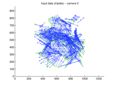
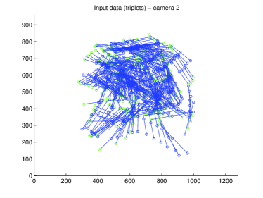
Figure 5: Example of input data for the tests (triplets of aligned LEDs in a rigid bar). Only the points are used in the calibration with the proposed algorithms. The triplet structure is used for evaluation purposes.

The sampling parameters in Algorithm 2 have been $M=N=50$, so that the cost function has been evaluated on $2\times 50\times 50=5000$ points. Figure 5 shows a sample of the input data for the calibration process. Figure 6 shows two views of the sampled points of the SLCV computed in Algorithm 2. Figure 7 displays the cost function (16) for this experiment, normalized and pseudo-colored from blue (0) to red (1). A logarithmic transformation has been applied to enhance the visualization of small costs. The reconstructed scene obtained with Algorithm 2 is shown in Fig. 8. Table 2 shows the reprojection error and the quotient between the standard deviation and the average of the segment lengths for each of the Euclidean upgrading techniques, before and after bundle adjustment.

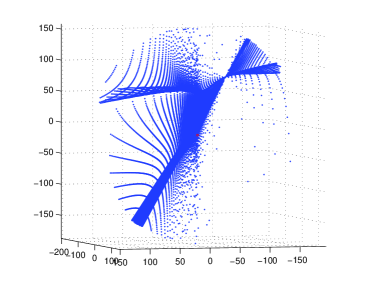
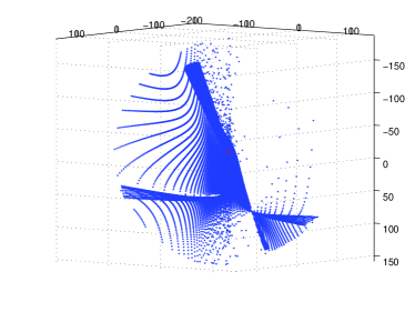
Figure 6: Two views of the sampled points of the SLCV.

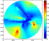
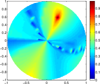
Figure 7: Experiment with the LED bar dataset: plots of the sampled cost function. Left: values at the unit disc of the complex plane, $|z|\leq 1$. Right: values at the complement of the unit disc, at positions $1/\bar{z}$. The white cross in the left plot marks the location of the minimum.

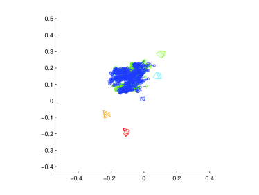
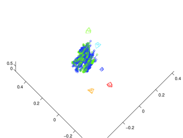
Figure 8: Two views of the 3D reconstruction in one of the experiments.

Table 2: Results of experiment comparing calibration techniques. The common previous projective calibration shows a reprojection error of $1.23$ pixels. $\sigma$ and $\mu$ are, respectively, the typical deviation and the average of LED bars lengths. SLCV sampling parameters: $N=M=50$.

	DAQ			SLCV			Triplets
	Euc. calib.	Euc. BA		Euc. calib.	Euc. BA		Euc. calib.	Euc. BA
Rep. error	$15.04$	$1.74$		$1.71$	$0.64$		$13.56$	$0.63$
$\sigma/\mu$	0.15	0.029		0.049	0.0098		0.026	0.0048

A second set of comparisons has been performed with two algorithms based on 3D search in the set of planes of space. The first of these algorithms is the one given in Hartley99 tailored to the case of square-pixel cameras and varying parameters. The second one makes use of a cost function based on the transfer of cyclic points using the candidate plane at infinity and is described in Algorithm 3.

Objective

Given the projective reconstruction of $N_{c}\geq 5$ cameras $\{\mathtt{P}^{k}\}_{k=1}^{N_{c}}$ and the coordinates $\boldsymbol{\pi}$ of a candidate plane at infinity, compute a cost of the fitting of the plane to the square-pixel constraints.

Algorithm

1. Transfer five selected imaged cyclic points to all images. These points are the projections of the points where $\boldsymbol{\pi}$ meets the isotropic lines (Appendix D) $\mathtt{L}_{j},j=1,\ldots,5$ of some selected cameras, i.e., $\mathbf{x}^{k}_{j}=\mathtt{P}^{k}\mathtt{L}_{j}\boldsymbol{\pi}$.

2. Compute the candidate IAC $\omega_{k}$ of each camera by fitting a conic to the set of five transferred points. This requires solving a system like (6), $\mathbf{x}^{k\top}_{j}\omega_{k}\mathbf{x}^{k}_{j}=0$, whose solution $\omega_{k}$ is the singular vector corresponding to the least singular value of the matrix of the system.

3. Measure the how far the obtained candidate IACs are from the square-pixel hypothesis. The cost is, based on (2), $c(\pi)=\sum_{k=1}^{N_{c}}\left(|\mathbf{I}^{\top}\omega_{k}\mathbf{I}|+|\bar{\mathbf{I}}^{\top}\omega_{k}\bar{\mathbf{I}}|\right)$, where $\mathbf{I}=(1,i,0)^{\top}$ and $\bar{\mathbf{I}}=(1,-i,0)^{\top}$.

Algorithm 3  Compute the cost of a candidate plane at infinity by transferring five cyclic points to all image planes and estimating the corresponding IACs of the cameras.

The compared methods search for the plane at infinity, but while Hartley99 and Algorithm 3 use a direct parameterization of $\boldsymbol{\pi}_{\infty}$ by its three coordinates in a quasi-affine reconstruction, the SLCV method reduces the dimension of the search space from three to two by searching over the surface (i.e., two-dimensional variety) of candidate planes at infinity in a general projective reconstruction.

It must first be pointed out that it has not been possible to obtain valid results with any of the 3D-search algorithms without previous obtainment of a quasi-affine reconstruction Hartley-Zisserman ; Hartley98 , an unnecessary step in the case of the presented SLCV-based algorithm. Table 3 compares the performance of the SLCV algorithm (without quasi-affine upgrading) with those of the two 3D search algorithms (with quasi-affine upgrading), using the LED bar data set. The three algorithms provide similar results for similar total number of points.

As for the computational cost of the three compared algorithms, the cost in the case of each iteration of the SLCV algorithm is the sum of the cost of the plane generation and the plane evaluation, both of which are comparable to the cost of plane evaluation in the two other algorithms.

Table 3: Experiment with five cameras viewing a moving LED bar. Results of search-based autocalibration algorithms with a posteriori square-pixel enforcement. $\sigma$ and $\mu$ are, respectively, the typical deviation and the average of LED bars lengths. $N$, $M$ have been chosen so that the number of samples is $2NM\approx N_{s}$.

# samples	$N_{s}=10^{3}$	$N_{s}=10^{3}$	$N=M=22$
Rep. error	10.34	2.57	1.97
$\sigma/\mu$	0.051	0.050	0.055
# samples	$N_{s}=20^{3}$	$N_{s}=20^{3}$	$N=M=63$
Rep. error	1.63	1.21	1.06
$\sigma/\mu$	0.032	0.032	0.035

5.2 Checkerboard dataset

The developed method has also been tested on a different set of 5 to 10 images that contain checkerboard patterns ronda08 . This calibration rig provides an additional validation of the results. The images, of size $1280\times 960$ pixels, were acquired with a Sony DSC-F828 digital camera. To test varying parameters, the equivalent focal length (in a 35 mm film) of the camera was set to 50 mm in eight of the images and to 100 mm in the remaining two. Variations due to auto-focus were not controlled. For this range of focal lengths, the lens distortion (radial and tangential) can be neglected, so it is assumed to be zero.

For each of the following experiments, scale-invariant key points (SIFT Lowe99 ) are detected and matched across images, obtained using SnavelySS08 . Then, a projective reconstruction of the scene is obtained, as already explained. Normalization of coordinates (“preconditioning”) is applied, as it is essential to improve the numerical conditioning of the equations in the different estimation problems involved (fundamental matrix, triangulation, resection and bundle adjustment). Table 4 summarizes the parameters of the projective reconstructions. The resulting set of projection matrices are the input to the autocalibration algorithms.

Table 4: Projective reconstructions.

Scene	Checkerboard		Plaza de la Villa
# images	10	5	16	5
# 3-D points	1494	1199	8555	1083
# image points	6660	4472	35181	3483
Rep. error (BA)	0.22268	0.17678	0.16053	0.17855

Table 5: Reprojection error and intrinsic parameter comparison for the experiment with 10 images of the Checkerboard scene. For each statistic, the top row corresponds to the value for cameras with $f=50$ mm (equivalent in 35 mm film) and the bottom row corresponds to cameras with $f=100$ mm. Data are given in pixels.

Method	AQC	DAQ	SLCV	Euc. BA
Mean focal length $\alpha$	1822.9	1851.4	1806.2	1847.8
	3433.2	3579.3	3399.4	3555.7
$\alpha$ standard deviation	10.95	4.86	16.1	7.77
	36.15	13.33	29.21	4.53
Mean pp $(u_{0,}v_{0})$	(623.1, 463.9)	(638.1, 477.8)	(607.4, 468.9)	(620.4, 485.3)
	(618.6, 446.8)	(654.5, 505.7)	(605.5, 455.4)	(588.0, 525.2)
p.p. std. dev.	(16.85, 8.13)	(1.61, 4.96)	(27.7, 11.15)	(6.72, 8.71)
	(34.44, 0.55)	(17.27, 10.91)	(53.18, 7.47)	(24.79, 6.36)
Rep. error	0.65765	0.27181	0.27497	0.22386

Table 5 shows the results for the experiment with 10 images. In this case, it is possible to compare the SLCV and DAQ algorithms to a technique based on the AQC Valdes04 . A Euclidean bundle adjustment with enforcement of the square-pixel condition is performed after the Euclidean calibration with each of the four compared techniques. The solution obtained (regardless of the AQC, DAQ or SLCV initialization), is given in the last column of Table 5.

If the image resolution and the size of the CCD of the camera are known, it is possible to convert the focal length from mm to pixels. For this dataset, an equivalent focal length of $f=50$ mm translates to $\alpha=1850$ pixels, which is very close to the values obtained by the different algorithms tested (first row of Table 5).

Because the DAQ algorithm yields good estimates of the intrinsic parameters (with small dispersion and reprojection error), we may conclude that the principal point (p.p.) of the camera is close to the center of the image. This observation is also supported by the estimates of the p.p. due to the other algorithms. All three autocalibration methods show a strong agreement with the three-homography calibration algorithm in ronda08 and (Hartley-Zisserman, , p. 211).

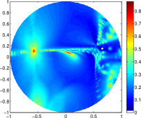
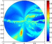
Figure 9: Experiment with 10 images of the Checkerboard dataset: plots of the sampled cost function. Left: values at the unit disc of the complex plane, $|z|\leq 1$. Right: values at the complement of the unit disc, at positions $1/\bar{z}$. The white cross in the left plot marks the location of the minimum.

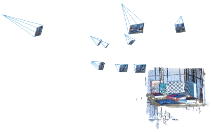
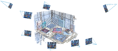
Figure 10: Experiment with 10 images of the Checkerboard dataset: reconstructed 3D scene.

Euclidean calibration by means of the developed technique (SLCV) provides competitive results with respect to the other methods (DAQ or AQC), but with a slightly bigger dispersion around the mean values. In normalized coordinates, the weights used in (17) to measure the goodness of fit of the IACs in Algorithm 2 are $\gamma_{1}=\gamma_{2}=\gamma_{3}=\gamma_{4}=1$. The sampling parameters in Algorithm 2 are $M=N=100$. Figure 9 shows the sampled cost function. Figure 10 shows two views of the densely reconstructed scene corresponding to the Euclidean calibration by means of the SLCV algorithm. The dense reconstruction was obtained by feeding the images and the Euclidean calibration of the cameras to the Patch-based Multi-view Stereo Software (PMVS) FurukawaP07 .

Figure 11: Experiment with 5 images of the Checkerboard dataset: reconstructed 3D scene.

Table 6: Reprojection error and intrinsic parameter comparison for experiment with 5 images of the Checkerboard dataset. Same notation as in Table 5. Both DAQ and SLCV methods yield good results.

Method	DAQ	SLCV	Euc. BA
Mean focal length $\alpha$	1833.3	1855.2	1883.1
	3511.2	3602.1	3662.9
$\alpha$ standard deviation	0.46	3.84	4.78
	16.24	7.90	26.15
Mean p.p. $(u_{0,}v_{0})$	(637.4, 478.9)	(624.5, 477.2)	(620.0, 500.2)
	(664.2, 493.3)	(618.0, 492.4)	(588.8, 569.5)
p.p. std. dev.	(0.72, 2.12)	(1.41, 1.48)	(8.72, 0.68)
	(28.61, 15.91)	(31.53, 20.03)	(12.3, 15.4)
Rep. error	0.26204	0.20134	0.17689

Table 7: Reprojection error and intrinsic parameter comparison for experiment with 5 expanded images of the Checkerboard dataset. Same notation as in Table 5. The SLCV method clearly outperforms the DAQ method if the principal point is not near the image center.

Method	DAQ	SLCV	Euc. BA
Mean focal length $\alpha$	3143.7	1827.2	1877.6
	25499.9	3516.0	3643.56
$\alpha$ standard deviation	29.28	3.87	5.37
	20080.2	5.30	22.69
Mean p.p. $(u_{0,}v_{0})$	(801.3, 516.4)	(622.6, 478.5)	(617.5, 500.6)
	(12192.1, -3639.6)	(626.0, 493.9)	(584.0, 571.8)
p.p. std. dev.	(261.1, 44.54)	(6.49, 0.92)	(7.54, 0.54)
	(23167.2, 9700.0)	(43.46, 7.4)	(15.97, 9.37)
Rep. error	3324.95	0.20725	0.17707

Next, an experiment with a subset of 5 images is carried out. To account for varying parameters, three of the images correspond to a focal length $f=50$ mm and the remaining two have $f=100$ mm. Table 4 shows the parameters of the projective reconstruction. Table 6 compares the Euclidean upgrading given by the DAQ and the SLCV algorithms. Both initializations converge to the same solution after Euclidean bundle adjustment (last column of Table 6). The SLCV method yields similar results to those of the DAQ method but requiring fewer equations per camera. The reconstructed scene corresponding to the Euclidean calibration by means of the SLCV algorithm is shown in Fig. 11. The SLCV method provides a sensible initialization to Euclidean bundle adjustment.

Next, we demonstrate the good performance of the developed method in case of decentered principal point. To do so, the previous 5 images of the Checkerboard dataset are extended to $1600\times 1200$ pixels from the upper-left corner. The principal point is, as seen in Table 5, near the point with coordinates $(640,480)$ pixels, which significantly differs from the new image center at $(800,600)$ pixels. A projective reconstruction of the scene is obtained, with 1197 3-D points, 4463 image projections and a reprojection error of 0.17699 pixels. Table 7 compares the Euclidean upgrading by the two autocalibration methods in Table 6. Because the hypothesis of known principal point (e.g. at the image center) is not satisfied, the DAQ method performs poorly. The SLCV method, however, yields the similar good results as in Table 6 because it solely relies on the square-pixel constraint. The last column of Table 7 shows the result after refining the SLCV Euclidean calibration by bundle adjustment.

5.3 Outdoor dataset

As an additional experiment, 16 images of the Plaza de la Villa in Madrid (see Fig. 12) were acquired with an Olympus E-620 digital camera at a resolution of $1280\times 960$ pixels. The focal length was set to $f=50$ mm ($\alpha=1850$ pixels) in half of the images and to $f=70$ mm ($\alpha=2590$ pixels) in the other half. Reconstructions were carried out with all images and with a subset of 5 images (with different focal lengths). The parameters of the projective reconstructions are summarized in Table 4. Figures 13 and 14 show reconstructions of the scene with 16 and 5 images, respectively, obtained by Euclidean upgrading with the SLCV method.

Figure 12: Two images of the outdoor (Plaza de la Villa) scene.

Figure 13: Experiment with 16 images of the outdoor dataset: reconstructed 3D scene.

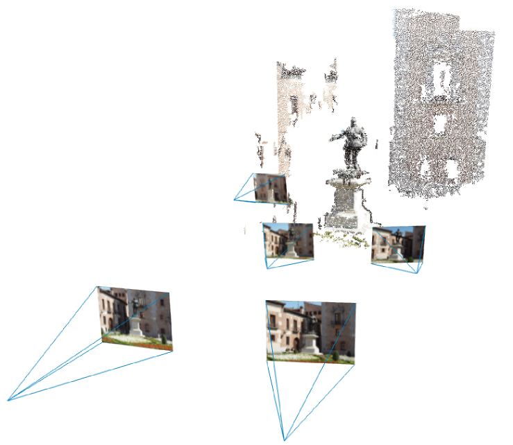
Figure 14: Experiment with 5 images of the outdoor dataset: reconstructed 3D scene.

6 Discussion

The search of the plane at infinity in a projectively reconstructed scene obtained with five or more square-pixel cameras is in principle a three-dimensional optimization problem. The SLCV concept allows to convert it into a two-dimensional optimization problem by restricting the search to the set of candidate planes that are compatible with the restrictions provided by a given subset of three of the cameras.

The empirical comparison of the SLCV algorithm performance with alternative 3D-search based algorithms presented in the results section points out two facts: First, the SLCV algorithm does provide valid results with different sets of real image data without previous preprocessing of the projective reconstruction, while for the tested 3D-search algorithms a previous quasi-affine upgrading seems to be mandatory. Second, the availability of this quasi-affine upgrading can be effective to the point of compensating for the larger dimension of the search space.

Summing up these to facts, we may conclude that the choice between the SLCV unrestricted 2D search and a cheirality constrained 3D search depends on the effectiveness of these constraints to narrow the search area, which in turn depends on the scene contents.

Although cheirality constraints have not yet been considered in the proposed algorithm, nothing prevents this integration and therefore it constitutes an interesting topic for future research. Two approaches are natural: If the convex hull of the camera centers and scene points intersects one of the camera principal planes, cheirality constraints emerge by restricting the search to the lines in this principal plane that do not intersect the convex hull. In any case, the search can be performed on the set of lines of any plane of space. For a general plane, each line will require the solution of a fifth-degree polynomial, while for a plane contained in the SLCV it suffices a fourth-degree polynomial that, as is well known, can be solved using a closed-form expression. Result 5 provides a wide source of such planes that can be used for this purpose.

7 Conclusions

In this paper we have proposed an algorithm to obtain a Euclidean reconstruction from the minimum possible number of cameras with known pixel shape but otherwise varying parameters, i.e., five cameras. To this purpose we have introduced, as our main tool, the geometric object given by the variety of conics intersecting six given spatial lines simultaneously (the six-line conic variety, SLCV). We have presented an independent and self-contained treatment including a procedure for the explicit computation of the equation of the SLCV defined by three cameras.

While the SLCV for six lines in generic position is, in general, a surface of degree 8, we have shown that this degree can be reduced to 5 in the case of the three pairs of isotropic lines of three finite square-pixel cameras. We have seen that a direct application of this result is the obtainment of the candidate planes at infinity in case two points at infinity are known.

We have seen that the fifth-degree SLCV has three singularities of multiplicity three. We have used this fact to obtain a computationally efficient parameterization of the SLCV that, if we have some additional data, permits the obtainment of the plane at infinity by means of a two-dimensional search. An algorithm has been proposed for the case in which two or more additional cameras are available.

Experiments with real images for the autocalibration of scenes with 5, 10 and 16 cameras have been given, showing the good performance of the SLCV technique. Particularly, in the case of fewer than 10 cameras, so that the AQC cannot be used, the SLCV method overcomes the limitation of the DAQ based technique for camera autocalibration with varying parameters, i.e., the need for known principal point. We have also included a comparison with two other algorithms based on 3D-search on the space of planes. Thus, the developed method seems to be a feasible approach to solve the autocalibration problem in the above situation without requiring previous initialization. Furthermore, we have shown that the SLCV method is also a sound alternative to other approaches that require 10 or more cameras or some knowledge of the principal point.

Appendix A Proof of Result 1

Proof

First note that if $D(\boldsymbol{\pi},\mathbf{a}_{1},\ldots,\mathbf{a}_{4})=0$, the points $\mathtt{L}_{i}\boldsymbol{\pi},\mathbf{a}_{j}$ lie on a quadric $Q$. By construction, the points $\mathtt{L}_{i}\boldsymbol{\pi}$ are also on the plane $\boldsymbol{\pi}$, and therefore they lie on the conic $\boldsymbol{\pi}\cap Q$.

Conversely, let us suppose that the points $\mathtt{L}_{i}\boldsymbol{\pi}$ lie on a conic $C$ contained in $\boldsymbol{\pi}$. Let us choose coordinates $(x,y,z,t)$ such that the plane $\boldsymbol{\pi}$ is given by the equation $t=0$. Let $C(x,y,z)=t=0$ be the equations of $C$. Any quadric $Q$ containing $C$ has an equation of the form

$$\alpha\,C(x,y,z)+t(ax+by+cz+dt)=0.$$

Given four points $\mathbf{a}_{j}=(x_{j},y_{j},z_{j},t_{j})^{\top}$, it is always possible to find some quadric $Q$ through them because the points lead to a linear homogeneous system of four equations in the five unknowns $a,b,c,d,\alpha$ which always admits at least one non-trivial solution. Since the $10$ points $\mathtt{L}_{i}\boldsymbol{\pi},\mathbf{a}_{j}$ lie on $Q$, we conclude that $D(\boldsymbol{\pi},\mathbf{a}_{1},\ldots,\mathbf{a}_{4})=0$. ∎

Appendix B Proof of Result 2

Proof

Any plane $\boldsymbol{\pi}$ through the point $\mathbf{a}_{1}$ is a trivial solution of $D=0$, since the seven points $\mathtt{L}_{1}\boldsymbol{\pi},\ldots,\mathtt{L}_{6}\boldsymbol{\pi},\mathbf{a}_{1}$ would lie on the plane $\boldsymbol{\pi}$ and therefore the ten points lie on the quadric given by $\boldsymbol{\pi}$ and the plane formed by points $\mathbf{a}_{2},\mathbf{a}_{3},\mathbf{a}_{4}$. Consequently, the planes through $\mathbf{a}_{1}$ produce a linear factor $\boldsymbol{\pi}^{\top}\mathbf{a}_{1}$ of $D$ and so do the planes through each of the three remaining points $\mathbf{a}_{j}$.

Let us denote $\mathtt{A}=(\mathbf{a}_{1},\ldots,\mathbf{a}_{4})$. Next we show that $\det\mathtt{A}$ also divides $D$. Since the determinant $\det\mathtt{A}$ is irreducible (Bocher, , p. 176) when regarded as a polynomial in the coordinates of the points $\mathbf{a}_{j}$, it is enough to show that $D$ vanishes whenever $\det\mathtt{A}=0$, i.e., when the points $\mathbf{a}_{j}$ are contained in some plane $\boldsymbol{\pi}^{\prime}$. In such case, the ten points $\mathtt{L}_{i}\boldsymbol{\pi}$, $i=1,\ldots,6$ and $\mathbf{a}_{j}$, $j=1,\ldots,4$, lie in the degenerate quadric $\boldsymbol{\pi}\cdot\boldsymbol{\pi}^{\prime}$ so that $D$ cancels. We have therefore the required factorization (9).

Let us now show that $F$ does not depend on the variables $\mathbf{a}_{j}$. The degree of the variables $\mathbf{a}_{j}$ on the left hand side of (9) is two because the vectors $\nu_{2}(\mathbf{a}_{j})$ are homogeneous quadratic in the entries of $\mathbf{a}_{j}$ and each of the $\nu_{2}(\mathbf{a}_{j})$ appears only once as a column of the determinant. On the right hand side of (9) we have the factor $\det\mathtt{A}$, which is homogeneous of degree one in each $\mathbf{a}_{j}$, and the factors $\boldsymbol{\pi}^{\top}\mathbf{a}_{j}$, which are also homogeneous of degree one. Therefore the remaining factor $F$ does not depend on the $\mathbf{a}_{j}$ since otherwise there would be a mismatch between the degrees of both sides of (9).

Finally, let us check that the equation $F(\boldsymbol{\pi})=0$ characterizes the planes intersecting the six lines in points of a conic. Now that we have proven factorization (9), it is trivial that if $F(\boldsymbol{\pi})=0$ then $D(\boldsymbol{\pi},\mathbf{a}_{1},\ldots,\mathbf{a}_{4})=0$ and, by Result 1, $\boldsymbol{\pi}$ is a plane intersecting the six lines in points of a conic. Conversely, if $\boldsymbol{\pi}$ intersects the six lines in points of a conic, the determinant $D$ vanishes for any $\mathbf{a}_{j}$. In particular, choosing any non-coplanar points $\mathbf{a}_{j}$ not in $\boldsymbol{\pi}$, so that $\det\mathtt{A}\not=0\not=\boldsymbol{\pi}^{\top}\mathbf{a}_{j}$, we conclude that $F(\boldsymbol{\pi})=0$. ∎

Appendix C Proof of Result 4

Proof

Let $l_{i},\bar{l}_{i}$ note the pair of lines through the optical center $\mathbf{C}_{i}$ and let $\mathtt{L}_{i}$, $\bar{\mathtt{L}}_{i}$ be their Plücker matrices. Also, let the corresponding principal planes be $\boldsymbol{\pi}_{i}$, $i=1,2,3$. Using Result 2 we have that

$$\begin{split}D&=\det\left(\nu_{2}(\mathtt{L}_{1}\boldsymbol{\pi}),\ldots,\nu_{2}(\bar{\mathtt{L}}_{3}\boldsymbol{\pi}),\nu_{2}(\mathbf{a}_{1}),\ldots,\nu_{2}(\mathbf{a}_{4})\right)\\ &=\det(\mathbf{a}_{1},\ldots,\mathbf{a}_{4})\,(\boldsymbol{\pi}^{\top}\mathbf{a}_{1})\cdots(\boldsymbol{\pi}^{\top}\mathbf{a}_{4})\,(\boldsymbol{\pi}^{\top}\mathbf{C}_{1})(\boldsymbol{\pi}^{\top}\mathbf{C}_{2})\\ &\qquad(\boldsymbol{\pi}^{\top}\mathbf{C}_{3})\,G(\boldsymbol{\pi}).\end{split}$$

Assuming that $\boldsymbol{\pi}_{1}$ is a generic principal plane, let the candidate planes be parameterized as $\boldsymbol{\pi}=\lambda\boldsymbol{\pi}_{1}+\mu\boldsymbol{\xi}$. Since $l_{1},\bar{l}_{1}$ are contained in $\boldsymbol{\pi}_{1}$ we have $\mathtt{L}_{1}\boldsymbol{\pi}_{1}=\bar{\mathtt{L}}_{1}\boldsymbol{\pi}_{1}=\mathbf{0}$ and therefore $\mathtt{L}_{1}\boldsymbol{\pi}=\mu\mathtt{L}_{1}\boldsymbol{\xi}$ and $\bar{\mathtt{L}}_{1}\boldsymbol{\pi}=\mu\bar{\mathtt{L}}_{1}\boldsymbol{\xi}$. Consequently

$$D(\lambda,\mu)=\mu^{4}\det\left(\nu_{2}(\mathtt{L}_{1}\boldsymbol{\xi}),\nu_{2}(\bar{\mathtt{L}}_{1}\boldsymbol{\xi}),\nu_{2}(\mathtt{L}_{2}\boldsymbol{\pi}),\ldots,\nu_{2}(\mathbf{a}_{4})\right).$$

On the other hand, since $\mathbf{C}_{1}$ in $\boldsymbol{\pi}_{1}$, we have $\mathbf{C}_{1}^{\top}\boldsymbol{\pi}=\mu\mathbf{C}_{1}^{\top}\boldsymbol{\xi}$, so

$$\begin{split}&\mu^{4}\det\left(\nu_{2}(\mathtt{L}_{1}\boldsymbol{\xi}),\nu_{2}(\bar{\mathtt{L}}_{1}\boldsymbol{\xi}),\nu_{2}(\mathtt{L}_{2}\boldsymbol{\pi}),\ldots,\nu_{2}(\mathbf{a}_{4})\right)\\ &=\mu\det(\mathbf{a}_{1},\ldots,\mathbf{a}_{4})\,(\boldsymbol{\pi}^{\top}\mathbf{a}_{1})\cdots(\boldsymbol{\pi}^{\top}\mathbf{a}_{4})\,(\boldsymbol{\xi}^{\top}\mathbf{C}_{1})(\boldsymbol{\pi}^{\top}\mathbf{C}_{2})\\ &\qquad(\boldsymbol{\pi}^{\top}\mathbf{C}_{3})\,G(\boldsymbol{\pi}).\end{split}$$

Using the genericity of $\boldsymbol{\pi}_{1}$ and choosing conveniently the points $\mathbf{a}_{j}$ we have that $\mathbf{C}_{2},\mathbf{C}_{3},\mathbf{a}_{j}$ not in $\boldsymbol{\pi}_{1}$ for $j=1,\ldots,4$, i.e., $\mu$ does not divide any linear factor besides $\boldsymbol{\pi}^{\top}\mathbf{C}_{1}$. Therefore $\mu^{3}$ divides $G(\lambda\boldsymbol{\pi}_{1}+\mu\boldsymbol{\xi})$ and so $\boldsymbol{\pi}_{1}$ is a singular point of $G$ of multiplicity three.

∎

Appendix D Calculation of the Isotropic Lines

The isotropic lines are the back-projection of the cyclic points at infinity $(1,\pm i,0)^{\top}$. Let us see how we can compute their Plücker matrices from the rows of the corresponding projection matrix $\mathtt{P}$. In a projective reference in which $\mathtt{P}=(\mathbf{p}_{1},\mathbf{p}_{2},\mathbf{p}_{3})^{\top}$, the back-projection of the cyclic points is given by those $\mathbf{X}$ in $\mathbb{P}^{3}$ such that

$$\mathtt{P}\mathbf{X}\sim(1,\pm i,0)^{\top}.$$

Therefore the cross-product

$$\mathtt{P}\mathbf{X}\times(1,\pm i,0)^{\top}=0,$$

or, equivalently, $\mathbf{X}$ satisfies the equations

$$\mathbf{p}_{3}^{\top}\mathbf{X}=0=(\mathbf{p}_{2}\pm i\mathbf{p}_{1})^{\top}\mathbf{X}.$$

Hence, the isotropic lines are defined by the intersection of the planes $\mathbf{p}_{3}$ and $\mathbf{p}_{2}\pm i\mathbf{p}_{1}$. Finally, their Plücker matrices are given by

$$\mathtt{L}=\mathtt{M}(\mathbf{p}_{3},\mathbf{p}_{2}+i\mathbf{p}_{1})^{\ast},\quad\bar{\mathtt{L}}=\mathtt{M}(\mathbf{p}_{3},\mathbf{p}_{2}-i\mathbf{p}_{1})^{\ast}$$

where $\mathtt{M}$ and the $\ast$ operator were defined in Section 3.1.

Appendix E Computation of Polynomial $H_{0}$

The polynomial $H_{0}(\lambda,\mu)=A_{0}\lambda^{2}+B_{0}\lambda\mu+C_{0}\mu^{2}$ in equation (15) can be computed as follows. Performing the coordinate change (14), the Plücker matrices of the lines $l_{i}$ are

$$\begin{split}\mathtt{L}_{1}&=\mathbf{C}_{1}\mathbf{q}^{\top}-\mathbf{q}\mathbf{C}_{1}^{\top}=\left(\begin{array}[]{cccc}0&0&0&-1\\ \vskip 6.0pt plus 2.0pt minus 2.0pt\cr 0&0&0&-i\\ \vskip 6.0pt plus 2.0pt minus 2.0pt\cr 0&0&0&0\\ \vskip 6.0pt plus 2.0pt minus 2.0pt\cr 1&i&0&0\end{array}\right),\\ \mathtt{L}_{2}&=\mathbf{C}_{2}\mathbf{p}_{2}^{\top}-\mathbf{p}_{2}\mathbf{C}_{2}^{\top}=\left(\begin{array}[]{cccc}0&0&-x_{{2}}&-x_{{2}}\\ \vskip 6.0pt plus 2.0pt minus 2.0pt\cr 0&0&-y_{{2}}&-y_{{2}}\\ \vskip 6.0pt plus 2.0pt minus 2.0pt\cr x_{{2}}&y_{{2}}&0&-z_{{2}}\\ \vskip 6.0pt plus 2.0pt minus 2.0pt\cr x_{{2}}&y_{{2}}&z_{{2}}&0\end{array}\right),\\ \mathtt{L}_{3}&=\mathbf{C}_{3}\mathbf{p}_{3}^{\top}-\mathbf{p}_{3}\mathbf{C}_{3}^{\top}=\left(\begin{array}[]{cccc}0&-x_{{3}}&x_{{3}}&-x_{{3}}\\ \vskip 6.0pt plus 2.0pt minus 2.0pt\cr x_{{3}}&0&z_{{3}}+y_{{3}}&-y_{{3}}\\ \vskip 6.0pt plus 2.0pt minus 2.0pt\cr-x_{{3}}&-y_{{3}}-z_{{3}}&0&-z_{{3}}\\ \vskip 6.0pt plus 2.0pt minus 2.0pt\cr x_{{3}}&y_{{3}}&z_{{3}}&0\end{array}\right),\end{split}$$

where the points $\mathbf{p}_{i}=(x_{i},y_{i},z_{i},0)^{\top}$ are the intersection of lines $l_{i}$ with the plane $\boldsymbol{\pi}_{4}=(0,0,0,1)^{\top}$. The Plücker matrices $\bar{\mathtt{L}}_{i}$ are just the complex conjugate of the matrices $\mathtt{L}_{i}$. Substituting in equation (7) and factoring out the trivial linear factors we obtain the polynomial $H_{0}(\alpha,\beta)$. Explicit formulas can be found in http://www.gti.ssr.upm.es/ jir/SLCV.html

References

- (1) Bôcher, M.: Introduction to Higher Algebra. Dover Phoenix Editions. Dover Publications (2004)
- (2) Bradski, G.: The OpenCV Library. Dr. Dobb’s Journal of Software Tools (2000)
- (3) Carballeira, P., Ronda, J.I., Valdés, A.: 3D reconstruction with uncalibrated cameras using the six-line conic variety. In: IEEE Int. Conf. Image Processing (ICIP), pp. 205–208 (2008)
- (4) Faugeras, O.: Three Dimensional Computer Vision. MIT Press (1993)
- (5) Faugeras, O.: Stratification of 3-D vision: projective, affine, and metric representations. Journal of the Optical Society of America A 12, 46,548–4 (1995)
- (6) Faugeras, O., Luong, Q., Maybank, S.: Camera self-calibration: Theory and experiments. In: Eur. Conf. Comput. Vis. (ECCV), Lecture Notes in Computer Science, vol. 588, pp. 321–334. Springer Berlin / Heidelberg (1992)
- (7) Faugeras, O., Luong, Q.T., Papadopoulou, T.: The Geometry of Multiple Images: The Laws That Govern The Formation of Images of A Scene and Some of Their Applications. MIT Press, Cambridge, MA, USA (2001)
- (8) Finsterwalder, S.: Die geometrischen grundlagen der photogrammetrie. Jahresbericht der Deutschen Mathematiker-Vereinigung 6, 1–42 (1897)
- (9) Furukawa, Y., Ponce, J.: Accurate, Dense, and Robust Multi-View Stereopsis. In: IEEE Conf. Comput. Vis. and Pattern Recognition (CVPR), pp. 1–8 (2007)
- (10) Hartley, R.: Projective reconstruction and invariants from multiple images. IEEE Trans. Pattern Anal. Mach. Intell. 16(10), 1036–1041 (1994)
- (11) Hartley, R., Gupta, R., Chang, T.: Stereo from uncalibrated cameras. In: IEEE Conf. Comput. Vis. and Pattern Recognition (CVPR), pp. 761–764 (1992)
- (12) Hartley, R., Zisserman, A.: Multiple View Geometry in Computer Vision, 2nd edn. Cambridge University Press (2003)
- (13) Hartley, R.I.: Chirality. Int. J. Comput. Vis. 26(1), 41–61 (1998)
- (14) Hartley, R.I., Hayman, E., de Agapito, L., Reid, I.: Camera Calibration and the Search for Infinity. IEEE Int. Conf. Comput. Vis. (ICCV) 1, 510 (1999)
- (15) Hemayed, E.: A survey of camera self-calibration. In: Proc. IEEE Conference on Advanced Video and Signal Based Surveillance, pp. 351–357 (2003)
- (16) Heyden, A., Åström, K.: Euclidean Reconstruction from Image Sequences with Varying and Unknown Focal Length and Principal Point. In: IEEE Conf. Comput. Vis. and Pattern Recognition (CVPR) (1997)
- (17) Longuet-Higgins, H.C.: A computer algorithm for reconstructing a scene from two projections. Nature 293, 133–135 (1981)
- (18) Lowe, D.: Object Recognition from Local Scale-Invariant Features. In: IEEE Int. Conf. Comput. Vis. (ICCV), pp. 1150–1157 (1999)
- (19) Luong, Q.T., Viéville, T.: Canonical representations for the geometries of multiple projective views. Comput. Vis. Image Underst. 64, 193–229 (1996)
- (20) Ma, Y., Soatto, S., Kosecka, J., Sastry, S.: An Invitation to 3-D Vision. Springer (2003)
- (21) Maybank, S.J., Faugeras, O.D.: A theory of self-calibration of a moving camera. Int. J. Comput. Vision 8(2), 123–151 (1992)
- (22) Mohr, R., Veillon, F., Quan, L.: Relative 3D Reconstruction Using Multiple Uncalibrated Images. In: IEEE Conf. Comput. Vis. and Pattern Recognition (CVPR), pp. 543–548 (1993)
- (23) Pollefeys, M., Gool, L.V.: A stratified approach to metric self-calibration. In: IEEE Conf. Comput. Vis. and Pattern Recognition (CVPR), pp. 407–412 (1997)
- (24) Pollefeys, M., Koch, R., van Gool, L.: Self-Calibration and Metric Reconstruction in spite of Varying and Unknown Internal Camera Parameters. Int. J. Comput. Vis. 1(32), 7–25 (1999)
- (25) Ponce, J., McHenry, K., Papadopoulo, T., Teillaud, M., Triggs, B.: On the Absolute Quadratic Complex and Its Application to Autocalibration. In: IEEE Conf. Comput. Vis. and Pattern Recognition (CVPR), vol. 1, pp. 780–787 (2005)
- (26) Quan, L.: Invariants of 6 points from 3 uncalibrated images. In: Eur. Conf. Comput. Vis. (ECCV), Lecture Notes in Computer Science, vol. 801, pp. 459–470. Springer-Verlag (1994)
- (27) Ronda, J.I., Valdés, A., Gallego, G.: Line Geometry and Camera Autocalibration. J. Math. Imaging Vis. 32(2), 193–214 (2008)
- (28) Schröcker, H.P.: Intersection Conics of Six Straight Lines. Beitr. Algebra Geom 46(2), 435–446 (2005)
- (29) Seo, Y., Heyden, A.: Auto-Calibration from the Orthogonality Constraints. In: 15th Int. Conf. Pattern Recognition, vol. 1, pp. 67–71 vol.1 (2000)
- (30) Snavely, N., Seitz, S.M., Szeliski, R.: Modeling the World from Internet Photo Collections. Int. J. Comput. Vis. 80(2), 189–210 (2008)
- (31) Sturm, P.: A Case Against Kruppa’s Equations for Camera Self-Calibration. IEEE Trans. Pattern Anal. Mach. Intell. 22(10), 1199–1204 (2000)
- (32) Sturm, P.: A historical survey of geometric computer vision. In: Computer Analysis of Images and Patterns, Lecture Notes in Computer Science, vol. 6854, pp. 1–8. Springer Berlin Heidelberg (2011)
- (33) Tresadern, P.A., Reid, I.D.: Camera calibration from human motion. Image Vision Comput. 26(6), 851–862 (2008)
- (34) Triggs, B.: The Geometry of Projective Reconstruction I: Matching Constraints and the Joint Image. In: Int. J. Comput. Vis., pp. 338–343 (1995)
- (35) Triggs, B.: Autocalibration and the Absolute Quadric. In: IEEE Conf. Comput. Vis. and Pattern Recognition (CVPR), pp. 609–614 (1997)
- (36) Triggs, B., McLauchlan, P., Hartley, R., Fitzgibbon, A.: Bundle Adjustment - A Modern Synthesis. In: Vision Algorithms: Theory and Practice, Lecture Notes in Computer Science, vol. 1883, pp. 153–177. Springer Berlin / Heidelberg (2000)
- (37) Valdés, A., Ronda, J.I., Gallego, G.: Linear camera autocalibration with varying parameters. In: IEEE Int. Conf. Image Processing (ICIP), vol. 5, pp. 3395–3398. Singapore (2004)
- (38) Valdés, A., Ronda, J.I., Gallego, G.: The Absolute Line Quadric and Camera Autocalibration. Int. J. Comput. Vis. 66(3), 283–303 (2006)