Generation of strong magnetic fields by $r$-modes in millisecond accreting neutron stars: induced deformations and gravitational wave emission

Abstract

Differential rotation induced by the $r$-mode instability can generate very strong toroidal fields in the core of accreting, millisecond spinning neutron stars. We introduce explicitly the magnetic damping term in the evolution equations of the $r$-modes and solve them numerically in the Newtonian limit, to follow the development and growth of the internal magnetic field. We show that the strength of the latter can reach large values, $B\sim 10^{14}$ G, in the core of the fastest accreting neutron stars. This is strong enough to induce a significant quadrupole moment of the neutron star mass distribution, corresponding to an ellipticity $|\epsilon_{\rm B}|\sim 10^{-8}$. If the symmetry axis of the induced magnetic field is not aligned with the spin axis, the neutron star radiates gravitational waves. We suggest that this mechanism may explain the upper limit of the spin frequencies observed in accreting neutron stars in Low Mass X-Ray Binaries. We discuss the relevance of our results for the search of gravitational waves.

I Introduction

The $r$-mode instability plays an important role in the physics of millisecond neutron stars NSs. It excites the emission of gravitational waves (GWs), which carry away spin angular momentum causing the star to spin down. It also gives rise to large scale mass drifts, particularly in the azimuthal direction, and to differential rotation Rezzolla et al. (2000); Rezzolla et al. (2001a, b); Sa and Tome (2005, 2006). Differential rotation in turn produces very strong toroidal magnetic fields inside the star and these fields damp the instability by tapping the energy of the modes. This mechanism has been investigated in the case of rapidly rotating, isolated, newly born neutron stars in Refs. Rezzolla et al. (2000); Rezzolla et al. (2001a, b); Abbassi et al. (2012) and in the case of accreting millisecond neutron and quark stars in Refs. Cuofano and Drago (2010); Bonanno et al. (2011). Magnetic fields deform the star and if the magnetic axis is not aligned with the rotation axis the NS undergoes free body precession. The deformation induced by the strong toroidal field is such that the symmetry axis of the precessing NS drifts on a timescale determined by its internal viscosity, eventually becoming an orthogonal rotator Cutler (2002). This is an optimal configuration for efficient GW emission, thus enhancing angular momentum losses from the NS.
In this work we resume the analysis in Ref. Cuofano and Drago (2010) about the growth of the internal magnetic fields in accreting millisecond neutron stars induced by $r$-modes. We account for the back-reaction of the generated magnetic field on the mode amplitude, by introducing the magnetic damping rate into the evolution equations.
We find that the GW emission due to the magnetic deformation grows secularly in accreting NSs, effectively limiting the growth of their spin frequency. In particular, this mechanism could naturally explain the observed cut-off above $730$ Hz in the distribution of spin frequencies of the faster accreting neutron stars in Low Mass X-Ray Binaries (LMXBs) Chakrabarty et al. (2003); Chakrabarty (2005).
Finally, we estimate the strain amplitude of the GW signal emitted from LMXBs in the local group of galaxies to establish their detectability with advanced LIGO and Virgo interferometers.
The paper is organized as follows: in Sec. II we write the r-mode equations taking into account also the magnetic damping rate; in Sec. III we discuss the magnetic deformation of the star and the associated gravitational-waves emission; in Sec IV we derive the expression of the magnetic damping rate; in Sec. V we discuss numerical solutions of the equations; in Sec. VI we deal with the evolutionary scenarios for accreting neutron stars; in Sec. VII we focus on the relevance of our results for the search of gravitational waves. Finally in Sec. VIII we summarize our conclusions.

II R-mode equations

We derive here the equations that describe the evolution of r-modes in a NS core with a pre-existing poloidal magnetic field, $B_{p}$, and the associated generation of an internal azimuthal field $B_{\phi}$. Following Ref. Wagoner (2002), the total angular momentum $J$ of a star can be decomposed into an equilibrium angular momentum $J_{*}$ and a canonical angular momentum $J_{c}$ proportional to the $r$-mode perturbation:

$$J=J_{*}(M,\Omega)+(1-K_{j})J_{c},\,\,\,\,\,\,\,\,\,\,\,\,\,J_{c}=-K_{c}\alpha^{2}J_{*}$$ (1)

where $K_{(j,c)}$ are dimensionless constants and $J_{*}\cong I_{*}\Omega$.
The canonical angular momentum obeys the following equation Cuofano and Drago (2010); Friedman and Schutz (1978):

$$dJ_{c}/dt= 2J_{c}\{F_{g}^{r}(M,\Omega)$$ (2)

$$-[F_{v}(M,\Omega,T_{v})+F_{m_{i}}(M,\Omega,B)]\}$$

where $F_{g}^{r}$ is the gravitational radiation growth rate of the $r$-mode, $F_{v}=F_{s}+F_{b}$ is the sum of the shear and bulk viscous damping rate and $F_{m_{i}}$ is the damping rate associated with the generation of an internal magnetic field. Finally, $T_{v}(t)$ is a spatially averaged temperature.
The total angular momentum satisfies the equation:

$$dJ/dt=2J_{c}F_{g}^{r}+\dot{J}_{a}(t)-I_{*}\Omega F_{m_{e}}$$ (3)

where $\dot{J}_{a}$ is the rate of variation of angular momentum due to mass accretion (we assume $\dot{J}_{a}=\dot{M}(GMR)^{1/2}$, see Ref. Andersson et al. (2002)) and $F_{m_{e}}$ is the magnetic braking rate associated to the external poloidal magnetic field. In this work we do not consider additional torques such as, e.g. the interaction between the magnetic field and the accretion disk. Combining Eqs. (2) and (3) we obtain the evolution equations of the r-mode amplitude $\alpha$ and of the angular velocity of the star $\Omega$:

$$\frac{d\alpha}{dt}= \alpha(F_{g}^{r}-F_{v}-F_{m_{i}})$$ (4)

$$+\alpha[K_{j}F_{g}^{r}+(1-K_{j})(F_{v}+F_{m_{i}})]K_{c}\alpha^{2}$$

$$-\frac{\alpha\dot{M}}{2\tilde{I}\Omega}\left(\frac{G}{MR^{3}}\right)^{\frac{1}{2}}+\frac{\alpha F_{m_{e}}}{2}$$

$$\frac{d\Omega}{dt}= -2K_{c}\Omega\alpha^{2}[K_{j}F_{g}^{r}+(1-K_{j})(F_{v}+F_{m_{i}})]$$ (5)

$$-\frac{\dot{M}\Omega}{M}+\frac{\dot{M}}{\tilde{I}}\left(\frac{G}{MR^{3}}\right)^{\frac{1}{2}}-\Omega F_{m_{e}}\;$$

where $I_{*}=\tilde{I}MR^{2}$ with $\tilde{I}=0.261$ for an n=1 polytrope and $K_{c}=9.4\times 10^{-2}$, see Ref. Owen et al. (1998). Our results turn out to be rather insensitive to the exact value of $K_{j}\sim 1$ (see Ref. Wagoner (2002)).
The classical $r$-mode equations are simply recovered from the above by neglecting the magnetic damping term, $F_{m_{i}}$. In this case, it is readily seen that the $r$-modes will grow only if the condition $F^{r}_{\rm g}>F_{\rm v}$ is satisfied, while viscosity keeps the NS stable against $r$-modes if this condition is reversed. This simple argument defines the classical instability window for $r$-modes, which is drawn in Fig. 1 as the thick dot-dashed curve.

Well inside the classical instability window, where viscosity is negligible, a new type of equilibrium can be reached. Eq. (4) and Eq. (5) indeed imply that the growth of $r$-modes can be quenched by the magnetic damping term, $F_{\rm m_{i}}$, when the condition $F_{g}^{r}\leq F_{m_{i}}$ holds. Since $F_{\rm g}^{r}=F_{\rm g}^{\rm r}(\Omega)$ and $F_{m_{i}}=F_{m_{i}}(\Omega,B)$, the equilibrium condition $F_{\rm g}^{r}=F_{m_{i}}$ implies a relation $\Omega=\Omega(B)$, which can be written as:

$$\nu_{cr} \approx 68\,\,B_{d,8}^{\,1/7}\,\,\bar{B}_{\phi,12}^{\,1/7}\,\,M^{-2/7}_{1.4}\,\,R_{10}^{-3/7}$$ (6)

where $B_{d,8}=(B_{d}/10^{8}\,\mbox{G})$, $\bar{B}_{\phi,12}=(\bar{B}_{\phi}/10^{12}\,\mbox{G})$, $M_{1.4}=(M/1.4\,M_{\odot})$, $R_{10}=(R/10\,\mbox{km})$.
Here, and in the following, $\nu$ indicates the NS spin frequency and $\bar{B}_{\phi}$ is an energy averaged, azimuthal magnetic field induced by the $r$-modes.

For a given combination of $({\rm B_{\rm d}},\bar{B}_{\phi})$, Eq. (6) represents the critical frequency above which the star is $r$-mode unstable even against the effect of the magnetic damping term. For a given value of the spin frequency, on the other hand, Eq. (6) tells us the minimal combination of field strengths required to damp the $r$-modes. With the value of $B_{d}$ fixed, $r$-modes are excited as long as $\bar{B}_{\phi}$ is lower than required by Eq. 6. They continue to generate further azimuthal field, until Eq. (6) is satisfied and the NS is eventually stabilized with respect to r-modes.

III Magnetic deformation and GW emission

We assume a NS with an internal poloidal field which is described by Ferraro’s solution Cuofano and Drago (2010); Ferraro (1954)

$$\mbox{{B}}^{in}(t=0)=$$ (7)

$$B_{d}\,\left[\left(-3\frac{r^{2}}{R^{2}}+5\right)\texttt{cos}\,\theta\,\mbox{{e}}_{r}+\left(6\frac{r^{2}}{R^{2}}-5\right)\,\texttt{sin}\,\theta\,\mbox{{e}}_{\theta}\right]\,.$$

where $B_{d}$ is the surface field strength at the stellar equator. This is matched to an exterior dipolar field aligned with the star spin axis

$$\mbox{{B}}^{ext}=B_{d}\frac{R^{3}}{r^{3}}(2\,\texttt{cos}\,\theta\,\mbox{{e}}_{r}+\,\texttt{sin}\,\theta\,\mbox{{e}}_{\theta})$$ (8)

As for the internal structure of the NS, it is widely accepted that protons will be superconducting at temperatures $T\lesssim 10^{9}$ K Baldo and Schulze (2007); Wasserman (2003), at least in a fraction of the NS core. To maintain focus on the salient properties of our scenario, we carry out here a detailed study of the growth of r-modes and of the azimuthal field in a normal fluid core. In Section VI.2 we consider the likely occurrence of a shell of superconducting protons in the outer core and assess its impact on our conclusions.
Once modes are excited at an initial time $t_{0}$, they induce azimuthal drift motions of fluid parcels in the NS core. Following Ref. Rezzolla et al. (2001a), the total angular displacement from the onset of the instability up to time $t$ reads

$$\Delta\tilde{x}^{\phi}(r,t)=\frac{2}{3}\left(\frac{r}{R}\right)k_{2}(\theta)\int_{t_{0}}^{t}\alpha^{2}(t^{\prime})\Omega(t^{\prime})dt^{\prime}+\mathcal{O}(\alpha^{3})\,\,\,\,\,\,\,\,\,$$ (9)

where $k_{2}(\theta)\equiv(1/2)^{7}(5!/\pi)(\texttt{sin}^{2}\theta-2\texttt{cos}^{2}\theta)$. Magnetic field lines are twisted and stretched by the shearing motions and a new field component, in the azimuthal direction, is generated accordingly. The relation between the new and the original magnetic field inside the star in the Lagrangian approach is Rezzolla et al. (2001a):

$$\frac{B^{j}}{\rho}(\tilde{\mbox{{x}}},t)=\frac{B^{k}}{\rho}(\mbox{{x}},t_{0})\frac{\partial\tilde{x_{j}}(t)}{\partial x^{k}(t_{0})}.$$ (10)

This equation implies that the radial dependence of the initial and final magnetic field is the same. Integrating over time the induction equation in the Eulerian approach one gets Rezzolla et al. (2001b):

$$\delta B^{\theta} \simeq \delta B^{r}\simeq 0$$ (11)

$$\delta B^{\phi}(r,t) \simeq B_{0}^{\theta}\int\dot{\phi}(t^{\prime})dt^{\prime}\simeq B_{0}^{\theta}\Delta\tilde{x}^{\phi}(r,t)$$ (12)

where $B^{\phi}$ is the toroidal component generated by the $r$-modes.

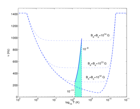
Figure 1: R-mode instability regions for NSs with strong internal fields. The $r$-mode instability window without internal magnetic field corresponds to the thick dotted-dashed line. The vertical dashed lines indicate the internal equilibrium temperatures of accreting neutron stars in LMXBs for, respectively, a maximum mass accretion rate $\dot{M}=10^{-8}\mbox{M}_{\odot}\mbox{yr}^{-1}$ (right) and a minimum value of $\dot{M}=10^{-11}\mbox{M}_{\odot}\mbox{yr}^{-1}$ (left). The instability window with a stable configuration of mixed poloidal-toroidal fields in the inner core, obtained from the condition $F_{g}^{r}=F_{m_{i}}+F_{\nu}$, is indicated by thin dotted-dashed lines. Three different values of the internal magnetic field are considered and we assume that poloidal and toroidal components have similar strengths. The light blue area indicates the region accessible to stable accreting NSs (see Sec. VI). The thick solid line indicates the maximum spin frequencies when the emission of gravitational waves due to the star’s deformation is taken into account ($\bar{B}_{\phi}\sim 10^{14}$ G, $|\epsilon_{B}|=10^{-8}$).

A toroidal field $B^{\phi}$ deforms a neutron star into a prolate ellipsoid with ellipticity

$$\epsilon_{B}\equiv\frac{I_{zz}-I_{xx}}{I_{zz}}$$ (13)

where $I_{jk}=\int_{V}\rho(r)(r^{2}\delta_{jk}-x_{j}x_{k})dV$ is the inertia tensor. For a neutron star with a normal core, this gives

$$\epsilon_{B}=-k_{\epsilon}\times 10^{-12}~{}R_{10}^{4}~{}M_{1.4}^{-2}~{}\bar{B}_{\phi,12}^{2}$$ (14)

where $k_{\epsilon}\simeq[0.5\mbox{--}5]$ is a parameter depending on the configuration of the internal fields Cutler (2002); Haskell et al. (2008); Mastrano et al. (2011).
In general, we expect the symmetry axis of the magnetic deformation not to be perfectly aligned with the rotation axis. In this situation, $J_{*}$ precesses around the symmetry axis with a period $P_{\rm prec}\simeq P/|\epsilon_{B}|$ Stella et al. (2005); Dall’Osso and Stella (2007); Dall’Osso et al. (2009), $P$ being the spin period of the star.
Due to the neutron star rotation, the relaxed state of its crust also has an intrinsic oblate deformation. This corresponds to the shape it would retain if the NS spin were stopped completely, without the crust cracking or re-adjusting in anyway. The ellipticity associated to this crustal reference deformation can be written as Cutler et al. (2003); Cutler (2002); Zdunik et al. (2008):

$$\epsilon_{\rm c}\approx k_{c}\times 10^{-8}\left(\frac{\nu_{\rm s}}{\rm kHz}\right)^{2}\,.$$ (15)

where $k_{c}\simeq[1\mbox{--}3]$ for an accreted crust Zdunik et al. (2008). As long as this is dominant, the NS effective mass distribution will be that of an oblate ellipsoid. In this case, the spin and symmetry axis of the freely precessing NS will tend to align. However, as the internal toroidal field grows, the ensuing magnetic deformation will at some point overcome the maximal oblateness that the crust can sustain (Eq. (15)). The NS first enters the r-mode instability window when its spin rate is $\nu_{\rm s,i}\gtrsim 150$ Hz. Therefore, the magnetic deformation will first become dominant when

$$|\epsilon_{\rm B}| \gtrsim 2\times 10^{-10}~{}k_{c}\left(\frac{\nu_{\rm s,i}}{150~{}\rm Hz}\right)^{2}\equiv\epsilon_{B,min}~{}~{}~{}{\rm~{}or}$$

$$\bar{B}_{\phi} \gtrsim 1.5\times 10^{13}\,\mbox{G}\left(\frac{k_{c}}{k_{\epsilon}}\right)^{1/2}\left(\frac{\nu_{\rm s,i}}{150\mbox{~{}Hz}}\right)\,M_{1.4}\,R^{-2}_{10}~{}.~{}~{}~{}~{}$$ (16)

Beyond this point, the total NS ellipticity becomes dominated by the magnetically-induced, prolate deformation. The freely precessing NS now becomes secularly unstable. In the presence of a finite viscosity of its interior, the wobble angle between the angular momentum $J_{*}$ and the symmetry (magnetic) axis grows until the two become orthogonal. This occurs on a dissipation (viscous) timescale, $\tau_{\rm v}$, which can be expressed as Cutler (2002)

$$\tau_{\rm v}=nP_{\rm prec}\simeq 10^{11}\times\left(\frac{n}{10^{5}}\right)\left(\frac{100~{}\rm{Hz}}{\nu_{s}}\right)\left(\frac{10^{-8}}{|\epsilon_{B}|}\right)\,\,\mbox{s}~{}~{}.$$ (17)

The parameter $n$ measures the dissipation timescale in units of the free precession cycle. Below, we determine quantitatively its role in promoting the orthogonalization of the NS symmetry and rotation axes. Given the significant theoretical uncertainties on the value of $n$, we normalize it to an educated guess Cutler (2002) but will consider it effectively as a free parameter.

An orthogonal rotator with a time-varying quadrupole moment, $Q_{22}\approx I_{*}\epsilon_{\rm B}$, emits gravitational-waves at a rate Shapiro and Teukolsky (1983)

$$\dot{E}_{\rm gw}^{B}=-\frac{32}{5}\frac{G(I_{*}\epsilon_{B})^{2}}{c^{5}}\Omega^{6}\,\,.$$ (18)

which produces spin down at the rate $F_{\rm g}^{\rm B}\equiv-(\dot{E}_{\rm gw}^{\rm B}/2E)$

$$F_{g}^{B}\simeq\frac{1}{5\times 10^{14}}\,\tilde{I_{1}}\,M_{1.4}~{}R_{10}^{2}\,\left(\frac{\epsilon_{\rm B}}{10^{-8}}\right)^{2}\,P_{-3}^{-4}~{}\mbox{s}^{-1}~{}$$ (19)

where $\tilde{I}_{1}=\tilde{I}/0.261$.
Therefore, if the orthogonality condition is satisfied, the NS looses significant spin angular momentum to GWs also through the induced magnetic deformation. This is accounted for by introducing the appropriate GW radiation term, $F^{\rm B}_{\rm g}$, in the Eq. (3), which now becomes:

$$dJ/dt=2J_{c}F_{g}^{r}+\dot{J}_{a}(t)-I_{*}\Omega(F_{g}^{B}+F_{m_{e}})\,\,.$$ (20)

Eq. (4) and Eq. (5) for the $r$-mode amplitude and the NS spin frequency are modified accordingly:

$$\frac{d\alpha}{dt}= \alpha(F_{g}^{r}-F_{v}-F_{m_{i}})$$ (21)

$$+\alpha[K_{j}F_{g}^{r}+(1-K_{j})(F_{v}+F_{m_{i}})]K_{c}\alpha^{2}$$

$$-\frac{\alpha\dot{M}}{2\tilde{I}\Omega}\left(\frac{G}{MR^{3}}\right)^{\frac{1}{2}}+\frac{\alpha(F_{g}^{B}+F_{m_{e}})}{2}\,,$$

$$\frac{d\Omega}{dt}= -2K_{c}\Omega\alpha^{2}[K_{j}F_{g}^{r}+(1-K_{j})(F_{v}+F_{m_{i}})]$$ (22)

$$-\frac{\dot{M}\Omega}{M}+\frac{\dot{M}}{\tilde{I}}\left(\frac{G}{MR^{3}}\right)^{\frac{1}{2}}-\Omega(F_{g}^{B}+F_{m_{e}}).~{}~{}$$

Eq. (21) and Eq. (22) now contain two terms for GW emission. Of these, $F^{B}_{g}$ is given by Eq. (19) while we adopt for $F^{r}_{g}$ the $r$-mode gravitational radiation reaction rate due to the $l=m=2$ current multipole Andersson and Kokkotas (2001)

$$F_{g}^{r}=\frac{1}{47}~{}M_{1.4}~{}R_{10}^{4}~{}P^{-6}_{-3}~{}~{}\mbox{s}^{-1}~{}~{}.$$ (23)

The evolution equations (21,22) will hold only after the symmetry axis of the azimuthal field has become orthogonal to the spin axis.
If $t$ measures the time since the generated magnetic field exceeds the critical value given by Eq. (16), the rotation of the magnetic axis will occur when $t\geq\tau_{\rm v}(t)$, where $\tau_{\rm v}$ is given by Eq. (17). Once the condition $t\geq\tau_{\rm v}(t)$ is met and Eq. (21) becomes effective, it is relevant to know which of the two GW emission terms is dominant. To see this, we consider the ratio between the GW torque due to r-modes, $\dot{J}_{g}^{r}=2J_{\rm c}F_{g}^{r}$, and the GW torque due to the magnetic deformation $\dot{J}_{g}^{B}=I_{*}\Omega F_{g}^{B}$ (see Eq. (20))

$$\frac{\dot{J}_{g}^{r}}{\dot{J}_{g}^{B}}\approx 2\times 10^{13}\,\alpha^{2}\,R_{10}^{2}\left(\frac{\epsilon_{B}}{10^{-8}}\right)^{-2}\,P^{-2}_{-3}$$ (24)

The magnetic deformation becomes dominant only when the $r$-mode amplitude gets very small, and the internal magnetic field accordingly large. In particular, the ratio in Eq. (24) becomes smaller than unity once $\alpha$ has decreased below the critical value:

$$\alpha_{\rm cr}\lesssim 2\times 10^{-7}\,R^{-1}_{10}\,\left(\frac{|\epsilon_{\rm B}|}{10^{-8}}\right)\,P_{-3}~{}~{}.$$ (25)

A numerical solution of Eqs. (21,22) is required to verify when the condition given by Eq. (25) is satisfied during the system’s evolution. Before calculating the evolution of $\alpha$ in detail, we note that a new asymptotic equilibrium could take place in this situation, with the material torque being balanced by the GW torque due to the magnetic deformation, $F_{\rm g}^{\rm B}$. This new equilibrium condition, $\dot{J}_{a}=\dot{J}_{g}^{B}$, leads to a limit spin frequency

$$\nu_{max}\approx 990~{}\tilde{I}_{1}^{-2/5}M_{1.4}^{-3/10}R_{10}^{-7/10}\,\left(\frac{\epsilon_{\rm B}}{10^{-8}}\right)^{-2/5}\,\dot{M}_{-8}^{1/5}~{}\mbox{Hz}$$ (26)

where $\dot{M}_{-8}=\dot{M}/(10^{-8}\,\rm M_{\odot}\,\rm{yr}^{-1})$.

IV Magnetic damping rate

Following Ref. Rezzolla et al. (2001b), we make use of Eq. (9) and Eq. (12) to derive the expression for the magnetic damping term. Let us first write the variation of the magnetic energy for a NS with a normal fluid core

$$\delta E_{M}\equiv\frac{1}{8\pi}\int_{V_{\infty}}\delta B^{2}dV$$ (27)

where $\delta B^{2}=(\delta B_{\hat{p}})^{2}+(\delta B_{\hat{\phi}})^{2}\simeq(\delta B_{\hat{\phi}})^{2}=B_{\hat{\phi}}^{2}$. In the last steps we have taken into account the Eqs. (11,12). The rate of variation of magnetic energy can be obtained from the Eqs. (9,12) and reads

$$\delta E_{M}^{N} \simeq \frac{2AB_{d}^{2}R^{3}}{9\pi}\left(\int_{0}^{t}\alpha^{2}(t^{\prime})\Omega(t^{\prime})dt^{\prime}\right)^{2}~{}.$$ (28)

From this the expression of the magnetic damping rate is derived Cuofano and Drago (2010):

$$F_{m_{i}}^{N} = \frac{(dE_{M}^{N}/dt)}{\tilde{E}}$$ (29)

$$\simeq \frac{4A}{9\pi\cdot(8.2\times 10^{-3})}\frac{B_{d}^{2}R\int^{t}_{0}\alpha^{2}(t^{\prime})\Omega(t^{\prime})dt^{\prime}}{M\Omega}\,\,\,\,\,\,\,\,\,\,\,$$

where $\tilde{E}\simeq 8.2\times 10^{-3}\alpha^{2}M\Omega^{2}R^{2}$ is the energy of the $r$-mode Rezzolla et al. (2001b) and $A\simeq 0.99$ Cuofano and Drago (2010). We make use of Eqs. (27) and (28) to estimate the toroidal magnetic field generated by r-modes

$$\bar{B}_{\phi}\simeq\left(\frac{4A}{3\pi}\right)^{1/2}B_{d}\int_{0}^{t}\alpha^{2}(t^{\prime})\Omega(t^{\prime})dt^{\prime}\,.$$ (30)

Note that $F_{\rm m_{i}}$ is not related to $\alpha$ in a simple way. The magnetic damping rate depends, like $B_{\hat{\phi}}$, on the integrated history of the $r$-mode amplitude since the star first entered the instability window (cfr. Eq. (12)).
Finally, by using the volume-averaged expression for the azimuthal field, $\bar{B}_{\phi}$, we can re-write the expression of the magnetic damping rate as

$$F_{m_{i}}^{N}\approx\frac{1}{6.67\times 10^{9}}\,R_{10}\,M_{1.4}^{-1}\,B_{d,8}\,\bar{B}_{\phi,12}\,P_{-3}~{}\mbox{s}^{-1}.~{}$$ (31)

V Numerical solutions

In the scenario we are describing, an initially slowly rotating NS is secularly spun up by mass accretion. When its spin frequency reaches a few hundred Hz, the NS enters the classical $r$-modes instability window. As the instability develops, the evolution of the $r$-mode amplitude becomes coupled to the growth of an internal, toroidal magnetic field. We now turn to a detailed numerical calculation of their coupled evolution, in the light of our previous discussion. This will help us clarify the sequence of events expected to occur as an accreting NS in a LMXB is secularly spun up by the material torque. In all our calculations we consider values of the mass accretion rate $\dot{M}=(10^{-8}\,\mbox{--}\,10^{-10})\,\mbox{M}_{\odot}\mbox{yr}^{-1}$. Note that, in accreting NSs, the mass accretion rate has an upper limit $\dot{M}_{\rm Edd}\sim 10^{-8}\mbox{M}_{\odot}\mbox{yr}^{-1}$ and most LMXBs do not accrete at this rate for a long time. Here $\dot{M}_{\rm Edd}$ is the mass accretion rate that produces the Eddington luminosity.

V.1 Numerical estimates of relevant rates

We begin by discussing the main physical quantities in the evolution equations that were not described in previous sections.
For non–superfluid matter the shear viscosity damping rate reads Andersson and Kokkotas (2001)

$$F_{s}=\frac{1}{6.7\times 10^{7}}M_{1.4}^{5/4}R_{10}^{-23/4}T^{-2}_{9}~{}~{}\mbox{s}^{-1}~{},$$ (32)

where $T_{9}=T/10^{9}$ K, while the bulk viscosity damping rate is given by Owen et al. (1998)

$$F_{b}=\frac{1}{6.99\times 10^{8}}\left(\frac{\Omega^{2}}{\pi G\bar{\rho}}\right)T_{9}^{6}~{},$$ (33)

which we can approximately rewrite as

$$F_{b}=\frac{1}{2.5\times 10^{9}}M^{-1}_{1.4}R_{10}^{3}P^{-2}_{-3}T^{6}_{9}\,\,\,\,\,\mbox{s}^{-1}\,.$$ (34)

However, for the temperatures of interest here the bulk viscosity damping rate is a few orders of magnitude smaller than the shear viscosity damping rate and therefore it is negligible.
Notice that viscous damping of the modes depends strongly on temperature, and that temperature will in turn be affected by viscous heating. It is thus important to describe accurately the global thermal balance of the NS. We consider three main factors: modified URCA cooling ($\dot{\epsilon}_{\rm u}$), shear viscosity reheating ($\dot{\epsilon}_{\rm s}$) and accretion heating ($\dot{\epsilon}_{\rm n}$). The equation of thermal balance of the star therefore reads:

$$\frac{d}{dt}\left[\frac{1}{2}C_{v}T\right]=-\dot{\epsilon}_{u}+\dot{\epsilon}_{s}+\dot{\epsilon}_{n}\,\,.$$ (35)

Here, C_v is the total heat capacity of the NS Watts and Andersson (2002):

$$C_{\rm v}=1.6\times 10^{39}M_{1.4}^{1/3}T_{9}\,\,\,\,\,\mbox{erg K}^{-1}.$$ (36)

The cooling rate due to the modified URCA reactions, $\dot{\epsilon}_{\rm u}$, reads Shapiro and Teukolsky (1983)

$$\dot{\epsilon}_{\rm u}=7.5\times 10^{39}M_{1.4}^{2/3}T_{9}^{8}\,\,\,\,\,\,\mbox{erg s}^{-1}\,.$$ (37)

If direct URCA processes can also take place, the NS cooling rate is expected to become much larger Blaschke et al. (2004). A recent phenomenological analysis of their implications can be found e.g. in Ref. Klähn et al. (2006). We assume, for simplicity, that only modified Urca processes are allowed in the NS core.
Dissipation of the $r$-mode oscillations by the action of shear viscosity will contribute to heating the NS. The corresponding heating rate, $\dot{\epsilon}_{\rm s}$, reads Andersson and Kokkotas (2001)

$$\dot{\epsilon}_{\rm s} = 2\alpha^{2}\Omega^{2}MR^{2}\tilde{J}F_{s}$$ (38)

$$= 8.3\times 10^{37}\alpha^{2}\Omega^{2}\tilde{J}M_{1.4}^{9/4}R_{10}^{-15/4}T_{9}^{-2}\,\,\,\,\,\,\mbox{erg s}^{-1}\,\,\,\,\,\,\,\,$$

where $\tilde{J}=1.635\times 10^{-2}$.
The accreting material exerts an extra pressure onto the NS crust causing direct compressional heating. The compression also triggers pycnonuclear reactions in the crust, which release further heat locally. The total heating rate, given by the sum of the two contributions, is Brown and Bildsten (1998) :

$$\dot{\epsilon}_{n}=\frac{\dot{M}}{m_{N}}\times 1.5\,\,\mbox{MeV}=4\times 10^{51}\dot{M}_{1.4}\,\,\,\,\,\mbox{erg s}^{-1}$$ (39)

where $m_{N}$ is the mass of a nucleon and $\dot{M}_{1.4}=\dot{M}/1.4M_{\odot}$ is measured in s^-1.

We can now solve self-consistently Eqs. (4,5,29,35), to obtain the evolution of the core temperature, $r$-mode amplitude and generated internal magnetic field, $\bar{B}_{\phi}$. We show in Fig. 2 the evolution of the $r$-mode amplitude, $\alpha$, after the star first enters the classical $r$-mode instability window. Three different values of accretion rate $\dot{M}$ and two values of the initial poloidal magnetic field $B_{d}$ are considered. We find that the maximum values of $\alpha$ are in the range $\alpha_{max}\sim[10^{-6}-10^{-4}]$.

In Fig. 3 we show the temporal evolution of the generated, volume averaged toroidal magnetic field. Also plotted are lines along which the condition $\tau_{\rm v}(t)=t$ is met, for different values of the parameter $n$. The secular velocity field associated to the $r$-modes, which is predominantly azimuthal, clearly induces very large secular effects. In particular, very strong toroidal magnetic fields, $\bar{B}^{\phi}\sim[10^{13}\mbox{--}10^{14}]$ G, can be produced by the wrapping of the pre-existing poloidal field lines, in $10^{4}-10^{6}$ yrs.

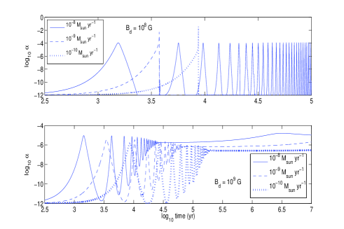
Figure 2: Temporal evolution of the r-mode amplitude $\alpha$ leaving out the instabilities of the magnetic fields. We consider three values of mass accretion rate $\dot{M}=(10^{-8},10^{-9},10^{-10})\,\mbox{M}_{\odot}\,\mbox{yr}^{-1}$ and two values of the initial poloidal magnetic field: $B_{d}=10^{8}$ G (upper panel) and $B_{d}=10^{9}$ G (lower panel).

The implications of these results for the spin equilibrium condition (Eq. (26)) will be discussed in the next section.

VI The overall evolutionary sequence: a general discussion

In the following we describe likely evolutionary scenarios for accreting ms spinning NSs, based on the numerical solutions and the physical discussion of the previous sections. We also consider implications of the possible occurrence of the Tayler instability in the strongly twisted internal field. Finally, the occurrence of proton superconductivity in (at least a fraction of) the NS core and its impact on our arguments are discussed.

Note that our analysis does not apply to compact stars in which exotic matter, like e.g. hyperons or deconfined quarks, is present in the inner core. In this type of stars the viscosity and thus the r-mode instability window is quite different from that of normal NSs Drago et al. (2008). Moreover, the evolution of the internal magnetic fields and the magnetic properties of the compact star are also expected to be different Bonanno et al. (2011); Alford et al. (2008).

VI.1 Normal Core

The growth rate of the azimuthal magnetic field once the accreting NS enters the r-mode instability window depends on the strength of the initial poloidal field $B_{d}$, and on the mass accretion rate $\dot{M}$.
In the most favorable cases, e.g. for $B_{d,8}=1$ and $\dot{M}_{-8}=(0.01-0.1)$, the magnetic field can reach a huge strength, $\bar{B}_{\phi}\approx 10^{14}$ G, in a few hundred years. In other cases, the internal magnetic field evolves on a much longer timescale up to million years (see discussion in Ref. Cuofano and Drago (2010)).

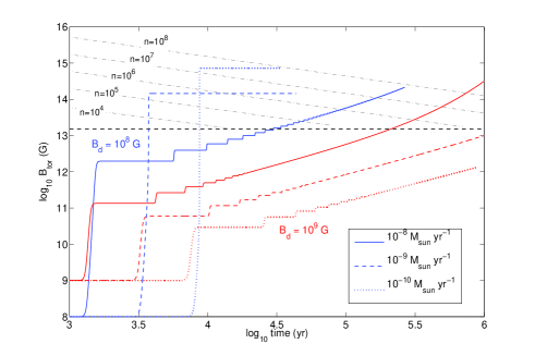
Figure 3: Temporal evolution of the generated toroidal magnetic field obtained by solving Eqs. (4,5). We considered three values of mass accretion rate $\dot{M}=(10^{-8},10^{-9},10^{-10})\,\mbox{M}_{\odot}\,\mbox{yr}^{-1}$ and two values of initial poloidal magnetic field $B_{d}=(10^{8},10^{9})$ G. The black dashed line indicates the minimal strength of the generated toroidal magnetic field for which the magnetic deformation becomes dominant (Eq. (16)). The time at which the rotation of the internal field takes place ($t=\tau_{\rm v}(t)$) is shown as a function of time for five values of the parameter $n=[10^{4}\mbox{--}10^{8}]$ (dashed-dotted gray lines). Except in cases with large values of initial poloidal fields $B_{d}\sim 10^{9}$ G and small values of mass accretion rate $\dot{M}<10^{-9}\,\mbox{M}_{\odot}\,\mbox{yr}^{-1}$, huge magnetic fields $B^{\phi}\sim[10^{13}\mbox{--}10^{14}]$ G are generated in less than $10^{6}$ years.

As already stated in Sec. III, the NS enters the $r$-mode instability window at $\nu_{\rm s,i}\gtrsim 150$. Hence, a minimal magnetic distortion $|\epsilon_{\rm B,min}|\approx 2\times 10^{-10}$ must be achieved for the magnetic deformation to overcome the crustal oblateness. This corresponds to a minimal azimuthal field $\bar{B}_{\phi,{\rm min}}\approx 10^{13}$ G. Only once this field strength is reached the star becomes secularly unstable. However, the magnetic axis is driven orthogonal to the spin axis in a time $\tau_{\rm v}$ (Eq. (17)). Therefore, the condition $\tau_{\rm v}(t)\leq t$ must also be satisfied for tilting of the magnetic axis to be effective. At the time at which both requirements are met, call it $t_{\rm ort}$, the toroidal magnetic field will have an intensity $B_{\phi,{\rm ort}}$ and, of course, $\tau_{\rm v}(t_{\rm ort})\leq t_{\rm ort}$.

After tilting, the original azimuthal field $B_{\phi,{\rm ort}}$ will have acquired an $r-\theta$ (poloidal) component, whose strength will be comparable to that of the new $\phi$-component. We assume that $\bar{B}_{\rm p,new}=\bar{B}_{\phi,{\rm new}}\approx(1/\sqrt{2})\bar{B}_{\phi,{\rm ort}}$, although the exact ratio will depend on the details of the distribution of the internal field.
Note that the generated magnetic fields may directly affect the r-mode oscillations when $B\gg 10^{14}$ G Lee (2005); Abbassi et al. (2012). We do not include this complicated back-reaction in our calculations. Our assumption will be justified a posteriori, since the maximum generated magnetic fields in our model reach values of order $10^{14}$ G.
In the following we will outline two possible evolutionary paths: which of the two will be followed by the star depends on the different combination of the parameters ($n$,$k_{\epsilon}$,$k_{c}$), on the mass accretion rate $\dot{M}$ and of the initial magnetic field $B_{d}$.

VI.1.1 Evolutionary Path ($\bar{B}_{\phi,ort}\gg\bar{B}_{\phi,min}$)

The first evolution path we discuss takes place if the condition $t\gtrsim\tau_{\rm v}$ is met when $B_{\phi,{\rm ort}}\gg B_{\phi,{\rm min}}$. In this case a very large deformation of the NS can be obtained. The main dissipation mechanism of these magnetic fields in the normal fluid core of neutron stars should be ambipolar diffusion whose timescale is given by Goldreich and Reisenegger (1992)

$$t_{amb}\sim 3\times 10^{9}\frac{T_{8}^{2}L_{5}^{2}}{B_{12}^{2}}~{}~{}\mbox{yr}~{},$$ (40)

where $L$ is the size of the region embedding the magnetic field and $L_{5}=L/10^{5}~{}\mbox{cm}$. Note that if $B_{\phi,{\rm ort}}\gg 10^{14}$ G the generated internal field would decay on a time shorter than a few million years to strengths of the order of $10^{14}$ G which correspond to a deformation $|\epsilon_{B}|\sim 10^{-8}$. The star is now stabilized with respect to r-modes up to frequencies $\nu_{\rm cr}\approx 950$ Hz (see Eq. (6)), but the maximum spin frequency is limited by GW emission due to the magnetic deformation (see Eq. (26)). The limiting frequency, for typical values of $\dot{M}\sim 10^{-9}M_{\odot}yr^{-1}$, corresponds to $\nu_{\rm max}\sim 630~{}\dot{M}_{-9}^{1/5}~{}(\epsilon_{B}/10^{-8})^{-2/5}$ Hz.

VI.1.2 Evolutionary Path ($\bar{B}_{\phi,ort}\approx\bar{B}_{\phi,min}$)

The second evolutionary path takes place if the condition $t\gtrsim\tau_{\rm v}$ is reached when $\bar{B}_{\rm\phi,ort}\approx\bar{B}_{\phi,{\rm min}}$. After the rotation of the magnetic axis, the GW emission term $F^{\rm B}_{\rm g}$ becomes effective, with $|\epsilon_{\rm B}|\approx\epsilon_{\rm B,min}$. The new magnetic field will have poloidal and toroidal components of comparable strength which stabilize the star against $r$-modes up to frequencies $\nu_{\rm cr}\approx 500$ Hz. Up to this frequency the magnetic deformation will thus be the only effective cause of GW emission.

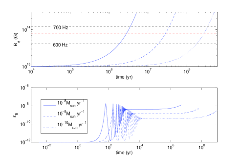
Figure 4: Upper panel: Temporal evolution of the generated toroidal magnetic field when the star enters again the r-mode instability window at frequencies $\nu_{cr}\approx 500$ Hz after the flip of the internal magnetic field ($B_{\phi,{\rm ort}}\approx B_{\phi,{\rm min}}\approx 10^{13}$ G). We show also the spin frequencies of the star (dashed black lines) obtained by Eq. (6). The red dashed line indicates the minimal strength of the generated toroidal magnetic field to have a new instability by magnetic deformation (Eq. (16)). Bottom panel: Temporal evolution of the r-mode amplitude $\alpha$ after the flip of the internal magnetic field. We consider three values of mass accretion rate $\dot{M}=(10^{-8},10^{-9},10^{-10})\,\mbox{M}_{\odot}\,\mbox{yr}^{-1}$.

Mass accretion will continue to spin up the star, which may eventually enter again the r-mode instability window thus starting the generation of new azimuthal field. In Fig. 4 we show the temporal evolution of the generated toroidal field and of the r-mode amplitude $\alpha$ (obtained by solving Eqs. (21,22)) when the star enters again the instability window at $\nu_{\rm s}\approx 500$ Hz. The magnetic fields can grow further and the star may be subject to a new instability when the magnetic field exceeds a value of the order of $10^{14}$ G at frequencies $\nu_{\rm s}\approx 650$ Hz (see Eq. (16) and Fig. 4).

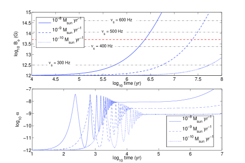
Figure 5: Upper panel: Temporal evolution of the generated toroidal magnetic field after the development of the Tayler instability. Here we assume $B_{d}=10^{12}$ G. We show also the spin frequencies of the star (dashed-dotted lines) obtained by Eq. (6). The red dashed line indicates the minimal strength of the generated toroidal magnetic field to have a new instability by magnetic deformation (Eq. (16)). Bottom panel: Temporal evolution of the r-mode amplitude $\alpha$ after the development of the Tayler instability. We consider three values of mass accretion rate $\dot{M}=(10^{-8},10^{-9},10^{-10})\,\mbox{M}_{\odot}\,\mbox{yr}^{-1}$.

After the second flip the evolution becomes similar to that described in the first scenario being again $B_{\phi,{\rm ort}}\approx 10^{14}$ G and $|\epsilon_{B}|\approx 10^{-8}$.

Tayler Instability

The issue of the stability of the magnetic field generated by $r$-modes still needs to be addressed. In the stably stratified environment of a stellar interior the Tayler instability (or pinch-type) is driven by the energy of the toroidal magnetic field. In a slowly rotating NS the instability is expected to set in at field strength $B_{\phi,\rm cr}\gtrsim 10^{12}$ G Spruit (1999); Cuofano and Drago (2010), with unstable modes growing approximately on the Alfvén time–scale as long as the ratio of the magnetic energy $E_{EM}$ to rotational kinetic energy $T_{rot}$

$$E_{EM}/T_{rot} \sim \frac{B^{2}R^{3}/3}{I\Omega^{2}/2}$$ (41)

$$\approx 2\times 10^{-8}\left(\frac{B}{10^{13}\,\mbox{G}}\right)^{2}\left(\frac{{\rm P}}{5\,\mbox{ms}}\right)^{2}$$

is greater than 0.2 Kiuchi et al. (2008).
In systems of interest to us, however, this ratio is expected to be extremely small, as shown by the estimate of Eq. (41). In this condition it is not clear at all that the Tayler instability will ever set in  Kiuchi et al. (2008); Lander and Jones (2011); Braithwaite (2009). It is interesting to briefly sketch the implications of this instability for the evolution of the magnetic fields in fast accreting compact stars.
The most important property of the Tayler instability in this context is that, after it develops, the toroidal component of the field produces, as a result of its decay, a new poloidal component which can itself be wound up, closing the dynamo loop Braithwaite (2006). When the differential rotation stops, the field can evolve into a stable configuration of a mixed poloidal-toroidal twisted-torus shape, with the two components having a comparable strength Reisenegger (2009); Braithwaite and Spruit (2006, 2004); Braithwaite and Nordlund (2006).
Here we assume that the Tayler instability develops in the Alfvén time–scale when $\bar{B}_{\phi}\sim 10^{12}$ G. At that point a poloidal field is generated, having a comparable strength, and the star is stable against $r$-modes only for frequencies slightly larger than 200 Hz. Mass accretion accelerates the star back into the instability region and a new toroidal field can then develop. The growth of the modes, and the generation of the new toroidal field, will start at a much higher initial poloidal field, say $B_{d}\approx 10^{12}$ G.
In Fig. 5 we show the evolution of the r-mode amplitude and of the magnetic field in this scenario, after the star re-enters the instability window.
The magnetic fields can grow further and the star may be subject to magnetic instability when $B_{\phi}\gtrsim 10^{14}$ G at frequencies $\nu_{\rm s}\approx 450$ Hz (see Eq. (16) and Fig. 5). After the flip of the internal magnetic field the evolution becomes once again similar to that described in the first scenario with $B_{\phi,{\rm ort}}\approx 10^{14}$ G and $|\epsilon_{B}|\approx 10^{-8}$.

VI.2 Superconducting layer

Protons in a NS core are expected to undergo a transition to a (type-II) superconducting state at temperatures $\lesssim 10^{9}$ K Baym et al. (1969). Recent calculations of the proton energy gap indicate that this transition should occur only in a limited density range in the outer core Baldo and Schulze (2007); Akgun and Wasserman (2008), corresponding to a spherical shell of thickness $\ell_{\rm s}=[1\mbox{--}3]$ km Baldo and Schulze (2007); Cuofano and Drago (2010). Accordingly, we assume protons in the inner core, a sphere of radius $R_{1}=R-\ell_{\rm s}$, to be in a normal (as opposed to superconducting) phase.

In a superconductor, components of the Maxwell stress tensor are enhanced by the ratio $H_{\rm c1}/B_{\rm s}$, with respect to a normal conductor Easson and Pethick (1977). Here $H_{\rm c1}\approx 10^{15}$ G is the lower critical field  and $B_{\rm s}$ is the magnetic induction within the superconductor, which is always $\ll H_{\rm c1}$ in a NS . Several authors thus suggested Jones (1975); Cutler (2002) that the deformation caused by a typical magnetic field $\sim 10^{12}~{}{\rm G}$ would be $\sim 10^{3}$ times larger than given by, e.g. Eq. (14). This would have very important implications for the scenario proposed here.

For a phase transition in a pre-existing magnetic field, Ref. Akgun and Wasserman (2008) argued that the magnetic induction in the superconducting outer core would be reduced with respect to that in the inner normal core, as required to maintain stress balance at the interface between the two regions. As a consequence, no significant change in the total NS ellipticity should be expected in this case.

In the context of the present work, the toroidal magnetic field is generated in the superconducting layer at the expenses of the $r$-mode energy. We thus expect that a larger deformation of the NS can be obtained only if a correspondingly larger amount of energy can be transferred from the modes to the toroidal field. Conversely, for a fixed energy transfer rate, one would expect a weaker field to be produced in the superconductor, such that the total magnetic stress - thus the induced deformation - would be the same as for a normal conductor.

A solution to the $r$-mode equations in an inhomogeneous star would be required to solve this problem self-consistently Cuofano and Drago (2010), which is beyond our scope here. However, we can gain some insight by considering the energy budget of the system.

We adopt the expression of the magnetic damping rate in the normal and superconducting case, following Rezzolla et al. (2001b) (cfr. Sec. III). For the normal fluid in the inner core, the rate of production of magnetic energy is (cfr. Eq. (31))

$$\frac{{\rm d}}{{\rm dt}}E^{({\rm N})}_{\rm M} = \frac{8}{45\pi}R_{1}\Phi_{\rm B}^{\rm N}~{}\bar{B}^{({\rm N})}_{\phi}(t)\frac{\Lambda^{{}^{\prime}}}{\Lambda}\,\alpha^{2}_{\rm N}(t)\,\Omega(t)~{}.$$ (42)

Here $\Lambda^{{}^{\prime}}$ and $\Lambda$ are angular integrals of order unity defined in Ref. Rezzolla et al. (2001b), $\Phi_{\rm B,0}$ is the initial magnetic flux threading the inner core and $\bar{B}^{({\rm N})}_{\phi}(t)$ is obtained by taking the volume average of the generated azimuthal field (cfr. Eq. (12)).

The superconducting layer has a volume $V^{({\rm SC})}=4\pi R^{2}_{1}\ell_{\rm s}$ and we can write

$$\frac{{\rm d}}{{\rm dt}}E^{({\rm SC})}_{\rm M} = \frac{H_{\rm c1}}{4\pi}V^{({\rm SC})}\frac{\Phi_{\rm B}^{SC}}{8\pi R^{2}_{1}}\frac{{\rm d}}{{\rm dt}}\Delta\tilde{x}^{\phi}$$ (43)

$$\approx \frac{H_{\rm c1}\Phi_{\rm B}^{SC}}{12\pi^{2}}\ell_{\rm s}\Lambda\alpha^{2}_{\rm SC}(t)\Omega(t)\,.$$

As the $r$-mode energy is tapped by the newly generated azimuthal field, the magnetic energy density and Maxwell stress grow both in the inner and outer core. We thus expect that stress balance at the interface between the two regions will play a role in the subsequent development of $r$-modes. To obtain the rates of magnetic energy density production $\dot{{\cal U}}_{\rm B}$ in either region we divide Eqs. (42,43) by the corresponding volumes, $V^{({\rm N})}$ and $V^{({\rm SC})}$. Hence

$$\frac{\dot{{\cal U}}^{({\rm N})}_{\rm B}}{\dot{{\cal U}}^{({\rm SC})}_{\rm B}}=\frac{\bar{B}^{({\rm N})}_{\phi}(t)}{H_{\rm c1}}\frac{dB^{({\rm N})}_{\phi}}{dB^{({\rm SC})}_{\phi}}\simeq\frac{\bar{B}^{({\rm N})}_{\phi}(t)}{H_{\rm c1}}\left[\frac{\alpha_{\rm N}(t)}{\alpha_{\rm SC}(t)}\right]^{2}~{},$$ (44)

having neglected numerical factors of order unity. If Maxwell stresses in the two zones need to meet an equilibrium condition, the above ratio should be of order unity. Accordingly, a stable evolution of the internal magnetic field requires that $\alpha_{\rm SC}/\alpha_{\rm N}\sim\,[\bar{B}^{({\rm N})}_{\phi}(t)/H_{\rm c1}]^{1/2}$. This relation can be considered as a boundary condition on the amplitude at the surface separating the normal and the superconducting region. If this condition on the $r$-mode amplitudes is not satisfied, we expect that the magnetic instabilities will affect the growth of $\alpha$ in the two zones acting to restore the stress balance. From this, we conclude that, if the condition of stress balance were to hold (at least in a time-average sense), azimuthal fields of different strengths would be generated in the two zones (see Eq. (44)), namely

$$B^{({\rm SC})}_{\phi}(t)\simeq\bar{B}^{({\rm N})}_{\phi}(t)\frac{\bar{B}^{({\rm N})}_{\phi}(t)}{H_{\rm c1}}$$ (45)

This implies that the total NS deformation is expected to be of the same order of the deformation in a normal conductor.
Note that superconducting protons may coexist with superfluid neutrons, in a fraction of the neutron star core. Pinning of neutron vortices to magnetic flux tubes may affect in this case both the growth of the magnetic field in the superconducting shell and the spin frequency evolution Alford and Good (2008); Glampedakis et al. (2011). However, this complicated interplay and its ultimate implications are still subject of much debate Srinivasan et al. (1990); Ruderman et al. (1998); Glampedakis and Andersson (2011) and the problem is far from settled. The coexistence of the two mutually interacting superfluid and superconducting particles of different species is still controversial, and notable observational limits on it have been proposed Link (2003). A detailed analysis of these effects and their inclusion in our numerical calculations are beyond the scope of this paper.

Discussion

The analysis of the previous scenarios allows us to draw some general conclusion about the internal magnetic fields and the maximum spin frequencies of the fastest accreting NSs. These conclusions are quite independent of the particular evolutionary path of the recycled stars. In the cases where $B_{\rm\phi,ort}\ll 10^{14}$ G and $\epsilon_{B}\approx\epsilon_{\rm min}$, the GW emission due to the magnetic deformation does not limit the spin frequency of the accreting stars that can re-enter the r-mode instability window and generate new azimuthal field. The new toroidal component can reach strengths $\bar{B_{\phi}}\gtrsim 10^{14}$ G causing a new magnetic instability. On the other hand, in the cases where $B_{\rm\phi,ort}\gg 10^{14}$ G the magnetic field rapidly decays by ambipolar diffusion to strengths again of order $10^{14}$ G. It is clear that an equilibrium configuration requires a value of the internal magnetic field $B_{\rm\phi,ort}\approx 10^{14}$ G with an $|\epsilon_{B}|\approx 10^{-8}$. This internal configuration limits the spin frequencies at values $\nu_{\rm max}\sim 630~{}\dot{M}_{-9}^{1/5}~{}(\epsilon_{B}/10^{-8})^{-2/5}$ Hz preventing the star from further increasing their magnetic field by re-entering the r-mode instability region. In Fig. 1 and Fig. 6 we show the limits on the maximum spin frequencies of accreting neutron stars as a function of temperature and of mass accretion rate respectively. In Fig. 6 we plot also the observational data of accreting millisecond pulsars and of burst oscillation sources. The fastest spin frequencies ($\nu\gtrsim 650$ Hz) can be reached only for mass accretion rates $\dot{M}\gtrsim 10^{-9}\,\rm M_{\odot}\rm yr^{-1}$ with a spin up time-scale in the range $\approx[10^{7}\mbox{--}10^{8}]$ yrs. Note that during this period of time, the internal magnetic field $B_{\rm\phi,ort}$ is not subject to significant decay.

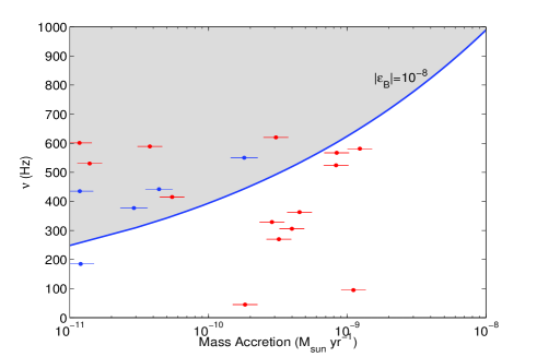
Figure 6: Limits on the maximum spin frequencies of accreting neutron stars with an ellipticity $|\epsilon_{B}|\sim 10^{-8}$ due to the magnetic deformation (solid line). We show also the fastest accreting millisecond pulsars (blue points) and the burst oscillation sources (red points) Watts et al. (2008). The stars can enter horizontally in the gray area when the mass accretion rate decreases down to values $\dot{M}<10^{-9}M_{\odot}\mbox{yr}^{-1}$ (see Discussion in Sec. VI).

Taking into account the maximum values of $\dot{M}$ for the NSs in LMXBs ($\approx 10^{-9}\rm\,M_{\odot}\,\rm yr^{-1}$) we can estimate a maximum spin frequency $\nu_{max}\lesssim 800$ Hz which is in agreement with the estimate $\nu_{max}\sim 730$ Hz of Refs. Chakrabarty et al. (2003); Chakrabarty (2005).

Note that the star can move horizontally in Fig. 6 entering the forbidden region (gray area) when the mass accretion rate decreases down to values $\dot{M}<10^{-9}M_{\odot}\mbox{yr}^{-1}$. An accreting spinning up neutron star is expected to move upwards in the white area in Fig. 6. When its spin frequency reaches the limiting value indicated by the solid line the star cannot spin up further and its position remains close to the limiting line. If subsequently the mass accretion diminishes, the star drift horizontally to the left Fig. 6. Therefore, in this interpretation, stars lying in the gray area of Fig. 6 are presently accreting at significant lower rate than in the past.

VII Detectability of the gravitational-waves emitted

In this section we discuss the detectability of the gravitational radiation emitted by recycled millisecond NSs due their magnetically-induced distortion. We consider a typical distance $d=10$ kpc of accreting NSs in our Galaxy and we calculate the average gravitational wave amplitude $h$.
The instantaneous signal strain can be expressed as Stella et al. (2005):

$$h\sim 1.5\times 10^{-29}\,\,k_{\epsilon}\,\,d_{10}^{-1}\,\,B_{\phi,13}^{2}\,\,\nu_{500}^{2}~{},$$ (46)

where $B_{\phi,13}=B_{\phi}/(10^{13}\mbox{~{}G})$, $d_{10}=d/(10\,\mbox{kpc})$ and $\nu_{500}=\nu/(500\,\mbox{Hz})$.
The spin frequency of accreting neutron stars changes significantly over a (long) timescale

$$\tau_{sv}\equiv\frac{\Omega}{\dot{\Omega}}\simeq\left[K_{m}\frac{\dot{M}}{\Omega}-{F_{g}^{B}}\right]^{-1}\gtrsim 10^{6}~{}\mbox{yr}~{},$$ (47)

where $K_{m}=(G/MR^{3})^{1/2}/\tilde{I}$. Hence we can integrate for long periods $T_{obs}$. The minimal detectable signal amplitude $h_{0}$ is Watts et al. (2008)

$$h_{0}\approx 11.4\sqrt{\frac{S_{n}}{T_{obs}}}$$ (48)

where $S_{n}$ is the power spectral density of the detector noise.

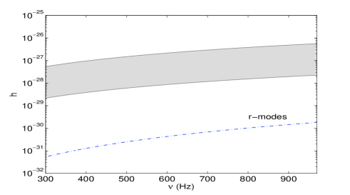
Figure 7: Averaged gravitational wave amplitude $h$ vs. the spin frequency of the star $\nu$. The gray area is obtained assuming that the accreting neutron star is located at a distance $d=10$ kpc and that the internal magnetic field is in the range $\bar{B}_{\phi}\approx[0.2\mbox{--}1]\times 10^{14}$ G and $k_{\epsilon}=1$. For comparison we show also the maximum amplitude of the GWs emitted by the star due to r-modes (dotted-dashed line) after the rotation of the internal magnetic field or the development of the Tayler instability. We assume that $\alpha\simeq 10^{-8}$ (see Figs. 4 and 5).

In Fig. 7 we show $h$ as a function of the spin frequencies $\nu$ of the star, while in Fig. 8 we compare the predicted and detectable amplitudes as a function of the frequency $f=2\,\nu$ of the signal.

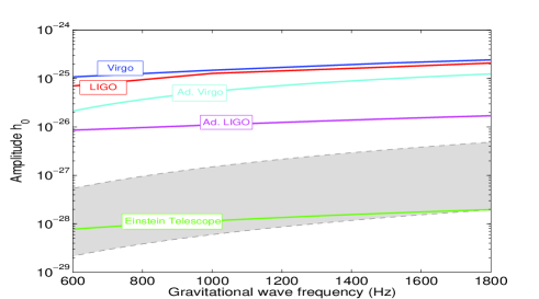
Figure 8: We compare the predicted amplitude (gray area) and the detectable amplitude for LIGO (2010) lig , Virgo vir , Advanced LIGO AdL , Advanced Virgo AdV and the Einstein Telescope et as a function of the frequency of the gravitational waves. Here we consider an integration time $T_{obs}=1$ yr. As in Fig. 7, $d=10$ kpc, $\bar{B}_{\phi}\approx[0.2\mbox{--}1]\times 10^{14}$ G and $k_{\epsilon}=1$.

We show also the sensitivity curve of LIGO and Virgo and of the next generation of detectors (Advanced LIGO, Advanced Virgo and Einstein Telescope).

VIII Conclusions

We have shown that accreting millisecond NSs can be deformed significantly by the very large magnetic fields generated by r-modes. A secular instability takes place when the magnetic distortion dominates over the maximal oblateness that the NS crust can sustain ($B_{\phi}\gtrsim 10^{13}$ G). As a consequence of this instability, the angular momentum $J_{*}$ and the magnetic axis become orthogonal on a timescale $\tau_{\rm v}$ given by Eq. (17) and the star begins to emit GWs.

We have shown that the GWs emission due to the magnetic deformation can limit the spin frequencies of accreting NSs. In particular we obtain a maximum spin frequency $\nu_{max}\lesssim 800$ Hz. Our results are quite independent of the exact evolution of the internal magnetic field, that is difficult to estimate and depends on several unknown parameters, e.g. the growth timescale of the Tayler instability and the parameter $n$ that is related to the flip time of the generated toroidal field.

In the end we analyzed the GWs emission due to the magnetic distortion. Our results suggest that with an integration time of $1$ year, the next generation of detectors (e.g. the Einstein Telescope) should be able to detect GW signals by accreting millisecond NSs located in our Galaxy.

References

- Rezzolla et al. (2000) L. Rezzolla, F. K. Lamb, and S. L. Shapiro, Astrophys. J. 531, L139 (2000).
- Rezzolla et al. (2001a) L. Rezzolla, F. K. Lamb, D. Markovic, and S. L. Shapiro, Phys. Rev. D64, 104013 (2001a).
- Rezzolla et al. (2001b) L. Rezzolla, F. K. Lamb, D. Markovic, and S. L. Shapiro, Phys. Rev. D64, 104014 (2001b).
- Sa and Tome (2005) P. M. Sa and B. Tome, Phys. Rev. D71, 044007 (2005).
- Sa and Tome (2006) P. M. Sa and B. Tome, Phys. Rev. D74, 044011 (2006).
- Abbassi et al. (2012) S. Abbassi, M. Rieutord, and V. Rezania, Mon.Not.Roy.Astron.Soc. 419, 2893 (2012).
- Cuofano and Drago (2010) C. Cuofano and A. Drago, Phys. Rev. D82, 084027 (2010).
- Bonanno et al. (2011) L. Bonanno, C. Cuofano, A. Drago, G. Pagliara, and J. Schaffner-Bielich, Astron.Astrophys. 532, A15 (2011).
- Cutler (2002) C. Cutler, Phys. Rev. D66, 084025 (2002).
- Chakrabarty et al. (2003) D. Chakrabarty et al., Nature 424, 42 (2003).
- Chakrabarty (2005) D. Chakrabarty, ASP Conf.Ser. 328, 279 (2005).
- Wagoner (2002) R. V. Wagoner, Astrophys. J. 578, L63 (2002).
- Friedman and Schutz (1978) J. L. Friedman and B. F. Schutz, Astrophys. J. 222, 281 (1978).
- Andersson et al. (2002) N. Andersson, D. I. Jones, and K. D. Kokkotas, Mon. Not. Roy. Astron. Soc. 337, 1224 (2002).
- Owen et al. (1998) B. J. Owen et al., Phys. Rev. D58, 084020 (1998).
- Ferraro (1954) V. C. A. Ferraro, Astrophys. J. 119, 407 (1954).
- Baldo and Schulze (2007) M. Baldo and H.-J. Schulze, Phys. Rev. C75, 025802 (2007).
- Wasserman (2003) I. Wasserman, Mon. Not. Roy. Astron. Soc. 341, 1020 (2003).
- Haskell et al. (2008) B. Haskell, L. Samuelsson, K. Glampedakis, and N. Andersson, Mon. Not. Roy. Astron. Soc. 385, 531 (2008).
- Mastrano et al. (2011) A. Mastrano, A. Melatos, A. Reisenegger, and T. Akgun, Mon.Not.Roy.Astron.Soc. 417, 2288 (2011).
- Stella et al. (2005) L. Stella, S. Dall’Osso, G. Israel, and A. Vecchio, Astrophys. J. 634, L165 (2005).
- Dall’Osso and Stella (2007) S. Dall’Osso and L. Stella, Astrophys.Space Sci. 308, 119 (2007).
- Dall’Osso et al. (2009) S. Dall’Osso, S. N. Shore, and L. Stella, Mon. Not. Roy. Astron. Soc. 398, 1869 (2009).
- Cutler et al. (2003) C. Cutler, G. Ushomirsky, and B. Link, Astrophys. J. 588, 975 (2003).
- Zdunik et al. (2008) J. L. Zdunik, M. Bejger, and P. Haensel, Astron. Astrophys. 491, 489 (2008).
- Shapiro and Teukolsky (1983) S. L. Shapiro and S. A. Teukolsky, Black holes, white dwarfs, and neutron stars: The physics of compact objects (1983).
- Andersson and Kokkotas (2001) N. Andersson and K. D. Kokkotas, Int. J. Mod. Phys. D10, 381 (2001).
- Watts and Andersson (2002) A. L. Watts and N. Andersson, Mon. Not. Roy. Astron. Soc. 333, 943 (2002).
- Blaschke et al. (2004) D. Blaschke, H. Grigorian, and D. N. Voskresensky, Astron. Astrophys. 424, 979 (2004).
- Klähn et al. (2006) T. Klähn, D. Blaschke, S. Typel, E. N. E. van Dalen, A. Faessler, C. Fuchs, T. Gaitanos, H. Grigorian, A. Ho, E. E. Kolomeitsev, et al., Phys. Rev. C74, 035802 (2006).
- Brown and Bildsten (1998) E. F. Brown and L. Bildsten, Astrophys. J. 496, 915 (1998).
- Drago et al. (2008) A. Drago, G. Pagliara, and I. Parenti, Astrophys. J. 678, L117 (2008).
- Alford et al. (2008) M. G. Alford, A. Schmitt, K. Rajagopal, and T. Schäfer, Reviews of Modern Physics 80, 1455 (2008).
- Lee (2005) U. Lee, Mon.Not.Roy.Astron.Soc. 357, 97 (2005).
- Goldreich and Reisenegger (1992) P. Goldreich and A. Reisenegger, Astrophys. J. 395, 250 (1992).
- Spruit (1999) H. C. Spruit, Astron. Astrophys. 349, 189 (1999).
- Kiuchi et al. (2008) K. Kiuchi, M. Shibata, and S. Yoshida, Phys. Rev. D78, 024029 (2008).
- Lander and Jones (2011) S. Lander and D. Jones, Mon.Not.Roy.Astron.Soc. 412, 1394 (2011).
- Braithwaite (2009) J. Braithwaite, Mon. Not. Roy. Astron. Soc. 397, 763 (2009).
- Braithwaite (2006) J. Braithwaite, Astron. Astrophys. 449, 451 (2006).
- Reisenegger (2009) A. Reisenegger, Astron. Astrophys. 499, 557 (2009).
- Braithwaite and Spruit (2006) J. Braithwaite and H. C. Spruit, Astron. Astrophys. 450, 1097 (2006).
- Braithwaite and Spruit (2004) J. Braithwaite and H. C. Spruit, Nature. 431, 819 (2004).
- Braithwaite and Nordlund (2006) J. Braithwaite and Å. Nordlund, Astron. Astrophys. 450, 1077 (2006).
- Baym et al. (1969) G. Baym, C. Pethick, and D. Pines, Nature (London) 224, 673 (1969).
- Akgun and Wasserman (2008) T. Akgun and I. Wasserman, Mon.Not.Roy.Astron.Soc. 383, 1551 (2008).
- Easson and Pethick (1977) I. Easson and C. J. Pethick, Phys. Rev. D16, 275 (1977).
- Jones (1975) P. B. Jones, Astrophys.Space Sci. 33, 215 (1975).
- Alford and Good (2008) M. G. Alford and G. Good, Phys. Rev. B 78, 024510 (2008).
- Glampedakis et al. (2011) K. Glampedakis, N. Andersson, and L. Samuelsson, Mon.Not.Roy.Astron.Soc. 410, 805 (2011).
- Srinivasan et al. (1990) G. Srinivasan, D. Bhattacharya, A. G. Muslimov, and A. J. Tsygan, Current Science 59, 31 (1990).
- Ruderman et al. (1998) M. Ruderman, T. Zhu, and K. Chen, Astrophys. J. 492, 267 (1998).
- Glampedakis and Andersson (2011) K. Glampedakis and N. Andersson, Astrophys. J. 740, L35 (2011).
- Link (2003) B. Link, Physical Review Letters 91, 101101 (2003).
- Watts et al. (2008) A. L. Watts, B. Krishnan, L. Bildsten, and B. F. Schutz, Mon.Not.Roy.Astron.Soc. 389, 839 (2008).
- (56) http://www.ligo.caltech.edu/~jzweizig/distribution/LSC_Data/.
- (57) https://wwwcascina.virgo.infn.it/senscurve/.
- (58) https://dcc.ligo.org/cgi-bin/DocDB/ShowDocument?docid=2974.
- (59) https://wwwcascina.virgo.infn.it/advirgo/.
- (60) http://www.et-gw.eu/etsensitivities#datafiles.