Efficient simulation of density and probability of large deviations of sum of random vectors using saddle point representations

Abstract

We consider the problem of efficient simulation estimation of the density function at the tails, and the probability of large deviations for a sum of independent, identically distributed, light-tailed and non-lattice random vectors. The latter problem besides being of independent interest, also forms a building block for more complex rare event problems that arise, for instance, in queuing and financial credit risk modeling. It has been extensively studied in literature where state independent exponential twisting based importance sampling has been shown to be asymptotically efficient and a more nuanced state dependent exponential twisting has been shown to have a stronger bounded relative error property. We exploit the saddle-point based representations that exist for these rare quantities, which rely on inverting the characteristic functions of the underlying random vectors. These representations reduce the rare event estimation problem to evaluating certain integrals, which may via importance sampling be represented as expectations. Further, it is easy to identify and approximate the zero-variance importance sampling distribution to estimate these integrals. We identify such importance sampling measures and show that they possess the asymptotically vanishing relative error property that is stronger than the bounded relative error property. To illustrate the broader applicability of the proposed methodology, we extend it to similarly efficiently estimate the practically important expected overshoot of sums of iid random variables.

1 Introduction

Let $(X_{i}:i\geq 1)$ denote a sequence of independent, identically distributed (iid) light tailed (their moment generating function is finite in a neighborhood of zero) non-lattice (modulus of their characteristic function is strictly less than one) random vectors taking values in $\Re^{d}$, for $d\geq 1$. In this paper we consider the problem of efficient simulation estimation of the probability density function of $\bar{X}_{n}=\frac{1}{n}\sum_{i=1}^{n}X_{i}$ at points away from $EX_{i}$, and the tail probability $P(\bar{X}_{n}\in\mathcal{A})$ for sets $\mathcal{A}$ that do not contain $EX_{i}$ and essentially are affine transformations of the non-negative orthant of $\Re^{d}$. We develop an efficient simulation estimation methodology for these rare quantities that exploits the well known saddle point representations for the probability density function of $\bar{X}_{n}$ obtained from Fourier inversion of the characteristic function of $X_{1}$ (see e.g., [4], [9] and [21]). Furthermore, using Parseval’s relation, similar representations for $P(\bar{X}_{n}\in\mathcal{A})$ are easily developed. To illustrate the broader applicability of the proposed methodology, we also develop similar representation for $E(\bar{X}_{n}:\bar{X}_{n}\geq a)$ in a single dimension setting $(d=1)$, for $a>EX_{i}$, and using it develop an efficient simulation methodology for this quantity as well.

The problem of efficient simulation estimation of the tail probability density function has not been studied in the literature, although, from practical viewpoint its clear that visual inspection of shape of such density functions provides a great deal of insight into the tail behavior of the sums of random variables. Another potential application maybe in the maximum likelihood framework for parameter estimation where closed form expressions for density functions of observed outputs are not available, but simulation based estimators provide an accurate proxy. The problem of efficiently estimating $P(\bar{X}_{n}\in\mathcal{A})$ via importance sampling, besides being of independent importance, may also be considered a building block for more complex problems involving many streams of i.i.d. random variables (see e.g., [23], for a queuing application; [16] for applications in credit risk modeling). This problem has been extensively studied in rare event simulation literature (see e.g., [5], [13], [15], [17], [25], [26]). Essentially, the literature exploits the fact that the zero variance importance sampling estimator for $P(\bar{X}_{n}\in\mathcal{A})$, though unimplementable, has a Markovian representation. This representation may be exploited to come up with provably efficient, implementable approximations (see [3] and [19]).

Sadowsky and Bucklew in [26] (also see [10]) developed exponential twisting based importance sampling algorithms to arrive at unbiased estimators for $P(\bar{X}_{n}\in\mathcal{A})$ that they proved were asymptotically or weakly efficient (as per the current standard terminology in rare event simulation literature, see e.g., [3] and [19] for an introduction to rare event simulation. Popular efficiency criteria for rare event estimators are also discussed later in Section 2.1). The importance sampling algorithms proposed by [26] were state independent in that each $X_{k+1}$ was generated from a distribution independent of the previously generated $(X_{i}:i\leq k)$. Blanchet, Leder and Glynn in [5] also considered the problem of estimating $P(\bar{X}_{n}\in\mathcal{A})$ where they introduced state dependent, exponential twisting based importance sampling distributions (the distribution of generated $X_{k+1}$ depended on the previously generated $(X_{i}:i\leq k)$). They showed that, when done correctly, such an algorithm is strongly efficient, or equivalently has the bounded relative error property.

The problem of efficient estimation of the expected overshoot $E\left[(\bar{X}_{n}-a):\bar{X}_{n}\geq a\right]$ is of considerable importance in finance and insurance settings. To the best of our knowledge, this is the first paper that directly tackles this estimation problem.

As mentioned earlier, in this article we exploit the saddle point based representations of the rare event quantities considered. These representations allow us to write the quantity of interest $\alpha_{n}$ as a product $c_{n}\times\beta_{n}$ where $c_{n}\sim\alpha_{n}$ (that is, $c_{n}/\alpha_{n}\rightarrow 1$ as $n\rightarrow\infty$) and is known in closed form. So the problem of interest is estimation of $\beta_{n}$, which is an integral of a known function. Note that $\beta_{n}\rightarrow 1$ as $n\rightarrow\infty$. In the literature, asymptotic expansions for $\beta_{n}$ exist, however they require computation of third and higher order derivatives of the log-moment generating function of $X_{i}$. This is particularly difficult in higher dimensions. In addition, it is difficult to control the bias in such approximations. As we note later in numerical experiments, these biases can be significant even when probabilities are as small as of order $10^{-9}$. In the insurance and financial industry, simulation, with its associated variance reduction techniques, is the preferred method for tail risk measurement even when asymptotic approximations are available (since these approximations are typically poor in the range of practical interest; see e.g., [16]).

In our analysis, we note that the integral $\beta_{n}$ can be expressed as an expectation of a random variable using importance sampling. Furthermore, the zero variance estimator for this expectation is easily ascertained. We approximate this estimator by an implementable importance sampling distribution and prove that the resulting unbiased estimator of $\alpha_{n}$ has the desirable asymptotically vanishing relative error property. More tangibly, the estimator of the integral $\beta_{n}$ has the property that its variance converges to zero as $n\rightarrow\infty$. An additional advantage of the proposed approach over existing methodologies for estimating $P(\bar{X}_{n}\in\mathcal{A})$ and related rare quantities is that while these methods require $O(n)$ computational effort to generate each sample output, our approach per sample requires small and fixed effort independent of $n$.

The use of saddle point methods to compute tail probabilities has a long and rich history (see e.g., [4], [20] and [21]). To the best of our knowledge the proposed methodology is the first attempt to combine the expanding literature on rare event simulation with the classical theory of saddle point approximations.

The rest of the paper is organized as follows: In Section 2 we briefly review the popular performance evaluation measures used in rare event simulation, and the existing literature on estimating $P(\bar{X}_{n}\in\mathcal{A})$. Then, in Section 3, we develop an importance sampling estimator for the density of $\bar{X}_{n}$ and show that it has asymptotically vanishing relative error. In Section 4, we devise an integral representation for $P(\bar{X}_{n}\in\mathcal{A})$ and develop an importance sampling estimator for it and again prove that it has asymptotically vanishing relative error. In this section we also discuss how this methodology can be adapted to similarly efficiently estimate $E(\bar{X}_{n}:\bar{X}_{n}\geq a)$ in a single dimension setting. In Section 5 we report the results of a few numerical experiments to support our analysis. We end with a brief conclusion and a discussion on some directions for future research in Section 6.

2 Rare event simulation, a brief review

Let $\alpha_{n}=E_{n}Y_{n}=\int Y_{n}dP_{n}$ be a sequence of rare event expectations in the sense that $\alpha_{n}\rightarrow 0$ as $n\rightarrow\infty$, for non-negative random variables $(Y_{n}:n\geq 1)$. Here, $E_{n}$ is the expectation operator under $P_{n}$. For example, when $\alpha_{n}=P(B_{n})$, $Y_{n}$ corresponds to the indicator of the event $B_{n}$.

Naive simulation for estimating $\alpha_{n}$ requires generating many iid samples of $Y_{n}$ under $P_{n}$. Their average then provides an unbiased estimator of $\alpha_{n}$. Central limit theorem based approximations then provide an asymptotically valid confidence interval for $\alpha_{n}$ (under the assumption that $E_{n}Y_{n}^{2}<\infty$).

Importance sampling involves expressing $\alpha_{n}=\int Y_{n}L_{n}d\tilde{P}_{n}=\tilde{E}_{n}[Y_{n}L_{n}]$, where $\tilde{P}_{n}$ is another probability measure such that $P_{n}$ is absolutely continuous w.r.t. $\tilde{P}_{n}$, with $L_{n}=\frac{dP_{n}}{d\tilde{P}_{n}}$ denoting the associated Radon-Nikodym derivative, or the likelihood ratio, and $\tilde{E}_{n}$ is the expectation operator under $\tilde{P}_{n}$. The importance sampling unbiased estimator $\hat{\alpha}_{n}$ of $\alpha_{n}$ is obtained by taking an average of generated iid samples of $Y_{n}L_{n}$ under $\tilde{P}_{n}$. Note that by setting

$$d\tilde{P}_{n}=\frac{Y_{n}}{E_{n}(Y_{n})}dP_{n}$$

the simulation output $Y_{n}L_{n}$ is $E_{n}(Y_{n})$ almost surely, signifying that such a $\tilde{P}_{n}$ provides a zero variance estimator for $\alpha_{n}$.

2.1 Popular performance measures

Note that the relative width of the confidence interval obtained using the central limit theorem approximation is proportional to the ratio of the standard deviation of the estimator divided by its mean. Therefore, the latter is a good measure of efficiency of the estimator. Note that under naive simulation, when $Y_{n}=I(B_{n})$ (For any set $D$, $I(D)$ denotes its indicator), the standard deviation of each sample of simulation output equals $\sqrt{\alpha_{n}(1-\alpha_{n})}$ so that when divided by $\alpha_{n}$, the ratio increases to infinity as $\alpha_{n}\rightarrow 0$.

Below we list some criteria that are popular in evaluating the efficacy of the proposed importance sampling estimator (see [3]). Here, $Var(\hat{\alpha}_{n})$ denotes the variance of the estimator $\hat{\alpha}_{n}$ under the appropriate importance sampling measure.

A given sequence of estimators $(\hat{\alpha}_{n}:n\geq 1)$ for quantities $(\alpha_{n}:n\geq 1)$ is said

• to be weakly efficient or asymptotically efficient if

  $$\limsup_{n\rightarrow\infty}\frac{\sqrt{Var(\hat{\alpha}_{n})}}{\alpha_{n}^{1-\epsilon}}<\infty$$

  for all $\epsilon>0$;

• to be strongly efficient or to have bounded relative error if

  $$\limsup_{n\rightarrow\infty}\frac{\sqrt{Var(\hat{\alpha}_{n})}}{\alpha_{n}}<\infty;$$

• to have asymptotically vanishing relative error if

  $$\lim_{n\rightarrow\infty}\frac{\sqrt{Var(\hat{\alpha}_{n})}}{\alpha_{n}}=0.$$

2.2 Literature review

Recall that $(X_{i}:i\geq 1)$ denote a sequence of independent, identically distributed light tailed random vectors taking values in $\Re^{d}$. Let $(X_{i}^{1},\ldots,X_{i}^{d})$ denote the components of $X_{i}$, each taking value in $\Re$. Let $F(\cdot)$ denote the distribution function of $X_{i}$. Denote the moment generating function of $F$ by $M(\cdot)$, so that

$$M(\theta):=E\left[e^{\theta\cdot X_{1}}\right]=E[e^{\theta_{1}X_{1}^{1}+\theta_{2}X_{1}^{2}+\cdots+\theta_{d}X_{1}^{d}}],$$

where $\theta=(\theta_{1},\theta_{2},\ldots,\theta_{d})$ and for $x,y\in\Re^{d}$ the Euclidean inner product between them is denoted by

$$x\cdot y:=x_{1}y_{1}+x_{2}y_{2}+\cdots+x_{d}y_{d}.$$

The characteristic function (CF) of $X_{i}$ is given by

$$\varphi(\theta):=E\left[e^{\iota\theta\cdot X_{1}}\right]=E[e^{\iota(\theta_{1}X_{1}^{1}+\theta_{2}X_{1}^{2}+\cdots+\theta_{d}X_{1}^{d})}]$$

where $\iota=\sqrt{-1}$. In this paper we assume that the distribution of $X_{i}$ is non-lattice, which means that $|\varphi(\theta)|<1$ for all $\theta\in\Re^{d}-\{0\}$.

Let $\Lambda(\theta):=\ln M(\theta)$ denote the cumulant generating function (CGF) of $X_{i}$. We define $\Theta$ to be the effective domain of $M(\theta)$, that is

$$\Theta:=\left\{\theta=(\theta_{1},\theta_{2},\ldots,\theta_{d})\in\Re^{d}|\Lambda(\theta)<\infty\right\}.$$

Throughout this article we assume that $0\in\Theta^{0}$, the interior of $\Theta$.

The large deviations rate function (see e.g., [11]) associated with $X_{i}$ is defined as

$$\Lambda^{*}(x)=\sup_{\theta\in\Re^{d}}(\theta\cdot x-\Lambda(\theta)).$$

This can be seen to equal $\tilde{\theta}\cdot x-\Lambda(\tilde{\theta})$ whenever there exists $\tilde{\theta}\in\Theta^{0}$ such that $\Lambda^{\prime}(\tilde{\theta})=x$. (Here, $\Lambda^{\prime}$ denotes the gradient of $\Lambda$). Now consider the problem of estimating $P(\bar{X}_{n}\in\mathcal{A})$. Let $dF_{\theta}(x)=\exp(\theta\cdot x-\Lambda(\theta))dF(x)$ denote the exponentially twisted distribution associated with $F$ when the twisting parameter equals $\theta$. Let $x_{0}$ denote the $\arg\min_{x\in\mathcal{A}}\Lambda^{*}(x)$. Furthermore, let $\theta^{*}\in\Theta^{0}$ solve the equation $\Lambda^{\prime}(\theta)=x_{0}$. Under the assumption that such a $\theta^{*}$ exists, [26] propose an importance sampling measure under which each $X_{i}$ is iid with the new distribution function $F_{\theta^{*}}$. Then, they prove that under this importance sampling measure, when $\mathcal{A}$ is convex, the resulting estimator of $P(\bar{X}_{n}\in\mathcal{A})$ is weakly efficient. See [3] and [19] for a sense in which this distribution approximates the zero variance estimator for $P(\bar{X}_{n}\in\mathcal{A})$. Since, $\Lambda^{\prime}(\theta^{*})=x_{0}$, it is easy to see that under the exponentially twisted distribution $F_{\theta^{*}}$, each $X_{i}$ has mean $x_{0}$.

As mentioned in the introduction, [5] consider a variant importance sampling measure where the distribution of $X_{j}$ depends on the generated $(X_{1},\ldots,X_{j-1})$. Modulo some boundary conditions, they choose an exponentially twisted distribution to generate $X_{j}$ so that its mean under the new distribution equals $\frac{1}{n-j+1}(nx_{0}-\sum_{i=1}^{j-1}X_{i})$. They prove that the resulting estimator is strongly efficient under the restriction that $\mathcal{A}$ is convex and has a twice continuously differentiable boundary. Later in Section 5, we compare the performance of the proposed algorithm to the one based on exponential twisting developed by [26] as well as with that proposed by [5].

3 Efficient estimation of probability density function of $\bar{X}_{n}$

In this section we first develop a saddle point based representation for the probability density function (pdf) of $\bar{X}_{n}$ in Proposition 1 (see e.g., [4], [9] and [21]). We then develop an approximation to the zero variance estimator for this pdf. Our main result is Theorem 1, where we prove that the proposed estimator has an asymptotically vanishing relative error.

Some notation is needed in our analysis. Let

$${\Re_{+}^{d}}:=\{(x_{1},x_{2},\ldots,x_{d})\in\Re^{d}|\,\,x_{i}\geq 0\,\,\,\forall i=1,2,\ldots d\}.$$

Denote the Euclidean norm of $x\in\Re^{d}$ by $|x|:=\sqrt{x\cdot x}$. For a square matrix $A$, $\text{det}(A)$ will denote the determinant of $A$, while norm of $A$ is denoted by

$$||A||:=\max_{|x|=1}|Ax|\,.$$

Let $\Lambda^{\prime\prime}(\theta)$ denote the Hessian of $\Lambda(\theta)$ for $\theta\in\Theta^{0}$. Whenever, this is strictly positive definite, let $A(\theta)$ be the inverse of the unique square root of $\Lambda^{\prime\prime}(\theta)$.

Proposition 1.

Suppose $\Lambda^{\prime\prime}(\theta)$ is strictly positive definite for some $\theta\in\Theta^{0}$. Furthermore, suppose that $|\varphi|^{\gamma}$ is integrable for some $\gamma\geq 1$. Then $f_{n}$, the density function of $\bar{X}_{n}$, exists for all $n\geq\gamma$ and its value at any point $x_{0}$ is given by:

$$f_{n}(x_{0})=\left(\frac{n}{2\pi}\right)^{\frac{d}{2}}\frac{\exp\left[n\left\{\Lambda(\theta)-\theta\cdot x_{0}\right\}\right]}{\sqrt{\text{det}(\Lambda^{\prime\prime}(\theta))}}\int_{v\in\Re^{d}}\psi(n^{-\frac{1}{2}}A(\theta)v,\theta,n)\times\phi(v)\,dv,$$ (1)

where

$$\psi(y,\theta,n)=\exp\left[n\times\eta(y,\theta)\right]$$

and

$$\eta(y,\theta)=\frac{1}{2}y^{t}\Lambda^{\prime\prime}(\theta)y+\Lambda\left(\theta+\iota y\right)-(\theta+\iota y)\cdot x_{0}-\Lambda(\theta)+\theta\cdot x_{0}.$$ (2)

Proof.

$$f_{n}(x_{0}) = \left(\frac{1}{2\pi}\right)^{d}\int_{t\in\Re^{d}}M_{\bar{X}_{n}}(\iota t)e^{-\iota(t\cdot x_{0})}\,dt\,\,\,\,[M_{\bar{X}_{n}}\,\,\text{is the MGF of}\,\bar{X}_{n}]$$

$$= \left(\frac{1}{2\pi}\right)^{d}\int_{t\in\Re^{d}}M^{n}\left(\frac{\iota t}{n}\right)e^{-\iota(t\cdot x_{0})}\,dt\,\,\,\,[M_{\bar{X}_{n}}\,\,\text{written in terms of}\,\,M]$$

$$= \left(\frac{n}{2\pi}\right)^{d}\int_{s\in\Re^{d}}M^{n}(\iota s)e^{-n\iota(s\cdot x_{0})}\,ds\,\,\,\,[\text{substituting}\,\,s=\frac{t}{n}]$$

$$= \left(\frac{n}{2\pi\iota}\right)^{d}\int_{\theta_{1}-\iota\infty}^{\theta_{1}+\iota\infty}\int_{\theta_{2}-\iota\infty}^{\theta_{2}+\iota\infty}\cdots\int_{\theta_{d}-\iota\infty}^{\theta_{d}+\iota\infty}e^{n[\Lambda(s)-s\cdot x_{0}]}\,ds_{1}ds_{2}\cdots ds_{d}$$

$$= \left(\frac{n}{2\pi\iota}\right)^{d}\int_{y\in\Re^{d}}\exp\left[n\left\{\Lambda(\theta+\iota y)-(\theta+\iota y)\cdot x_{0}\right\}\right]\,(\iota)^{d}dy$$

$$= \left(\frac{n}{2\pi}\right)^{d}\exp\left[n\left\{\Lambda(\theta)-\theta\cdot x_{0}\right\}\right]\int_{y\in\Re^{d}}\psi(y,\theta,n)\times\exp\left\{-n\frac{1}{2}y^{t}\Lambda^{\prime\prime}(\theta)y\right\}\,dy$$

$$= \left(\frac{n}{2\pi}\right)^{\frac{d}{2}}\exp\left[n\left\{\Lambda(\theta)-\theta\cdot x_{0}\right\}\right]\int_{w\in\Re^{d}}\psi(n^{-\frac{1}{2}}w,\theta,n)\times\phi(A(\theta)^{-1}w)\,dw$$ (5)

$$= \left(\frac{n}{2\pi}\right)^{\frac{d}{2}}\frac{\exp\left[n\left\{\Lambda(\theta)-\theta\cdot x_{0}\right\}\right]}{\sqrt{\text{det}(\Lambda^{\prime\prime}(\theta))}}\int_{v\in\Re^{d}}\psi(n^{-\frac{1}{2}}A(\theta)v,\theta,n)\times\phi(v)\,dv\,,$$ (6)

where the equality in (3), which holds for all $n\geq\gamma$, is the inversion formula applied to the characteristic function of $\bar{X}_{n}$ (see e.g, [14]). The assumption that $|\varphi|^{\gamma}$ is integrable ensures that $|M(\frac{\iota t}{n})|^{n}$, which is the characteristic function of $\bar{X}_{n}$, is an integrable function of $t$ for all $n\geq\gamma$. The equality in (3) holds, by Cauchy’s theorem, for any $\theta=(\theta_{1},\theta_{2},\ldots,\theta_{d})$ in the interior of $\Theta$. The substitution $y=n^{-\frac{1}{2}}w$ gives (5), while (6) follows from (5) by the substitution $w=A(\theta)v$. ∎

For a given $x_{0}\in\Re^{d},x_{0}\neq EX_{1}$, suppose that the solution $\theta^{*}$ to the equation $\Lambda^{\prime}(\theta)=x_{0}$ exists and $\theta^{*}\in\Theta^{0}$. Then, the expansion of the integral in (1) is available. For example, the following is well-known:

Proposition 2.

Suppose $\Lambda^{\prime\prime}(\theta^{*})$ is strictly positive definite and $|\varphi|^{\gamma}$ is integrable for some $\gamma\geq 1$. Then,

$$\int_{v\in\Re^{d}}\psi(n^{-\frac{1}{2}}A(\theta^{*})v,\theta^{*},n)\times\phi(v)\,dv=1+o\left(\frac{1}{\sqrt{n}}\right)\,.$$ (7)

A proof of Proposition 2 can be found in [21] (see also [14]). For completeness we include a proof in the Appendix. It is also useful in following proof of Proposition 3. The proof uses the estimates (32), (33), (34) and Lemma 1 developed later in this section.

3.1 Monte Carlo estimation

The integral in (1) may be estimated via Monte Carlo simulation. In particular, this integral may be re-expressed as

$$\int_{v\in\Re^{d}}\psi(n^{-\frac{1}{2}}A(\theta^{*})v,\theta^{*},n)\frac{\phi(v)}{g(v)}g(v)\,dv\,,$$

where $g$ is a density supported on $\Re^{d}$. Now if $V_{1},V_{2},\ldots,V_{N}$ are iid with distribution given by the density $g$, then

$$\hat{f}_{n}(\bar{x}):=\left(\frac{n}{2\pi}\right)^{\frac{d}{2}}\frac{\exp\left[n\left\{\Lambda(\theta^{*})-\theta^{*}\cdot x_{0}\right\}\right]}{\sqrt{\text{det}(\Lambda^{\prime\prime}(\theta^{*}))}}\frac{1}{N}\sum_{i=1}^{N}\frac{\psi(n^{-\frac{1}{2}}A(\theta^{*})V_{i},\theta^{*},n)\phi(V_{i})}{g(V_{i})}$$ (8)

is an unbiased estimator for $f_{n}(x_{0})$.

3.1.1 Approximating the zero variance estimator

Note that to get a zero variance estimator for the above integral we need

$$g(v)\varpropto\psi(n^{-\frac{1}{2}}A(\theta^{*})v,\theta^{*},n){\phi(v)}\,.$$

We now argue that

$$\psi(n^{-\frac{1}{2}}A(\theta^{*})v,\theta^{*},n)\sim 1$$ (9)

for all $v=o(n^{\frac{1}{6}})$. We may then select an IS density $g$ that is asymptotically similar to $\phi$ for $v=o(n^{\frac{1}{6}})$. In the further tails, we allow $g$ to have fatter power law tails. This ensures that large values of $V$ in the simulation do not contribute substantially to the variance.

Further analysis is needed to see (9). Note from the definition of $\eta(v,\theta)$, that

$$\eta(0,\theta)=0,\,\,\,\,\eta^{\prime\prime}(0,\theta)=0\,\,\,\,\text{and}\,\,\,\eta^{\prime\prime\prime}(v,\theta)=(\iota)^{3}\Lambda^{\prime\prime\prime}(\theta+\iota v)$$ (10)

for all $\theta$, while

$$\eta^{\prime}(0,\theta^{*})=0$$ (11)

for the saddle point $\theta^{*}$. Here $\eta^{\prime}$ , $\eta^{\prime\prime}$ and $\eta^{\prime\prime\prime}$ are the first, second and third derivatives of $\eta$ w.r.t. $v$, with $\theta$ held fixed. Note that while $\eta^{\prime}$ and $\eta^{\prime\prime}$ are $d$-dimensional vector and $d\times d$ matrix respectively, $\eta^{\prime\prime\prime}(v,\theta)$ is the array of numbers: $((\frac{\partial^{3}\eta}{\partial v_{i}\partial v_{j}\partial v_{k}}(v,\theta)))_{1\leq i,j,k\leq d}$.

The following notation aids in dealing with such quantities: If $A=(a_{ijk})_{1\leq i,j,k\leq d}$ is a $d\times d\times d$ array of numbers and $u=(u_{1},u_{2},\ldots,u_{d})$ is a $d$-dimensional vector and $B$ is a $d\times d$ matrix then we use the notation

$$A\odot u=\sum_{1\leq i,j,k\leq d}a_{ijk}u_{i}u_{j}u_{k}$$

and

$$A\star B=(c_{ijk})_{1\leq i,j,k\leq d}\,\,,$$

where

$$c_{ijk}=\sum_{m,n,p}a_{mnp}b_{mi}b_{nj}b_{pk}\,.$$

Following identity is evident:

$$A\odot(Bu)=(A\star B)\odot u\,.$$ (12)

Since, it follows from the three term Taylor series expansion and (10,11) above, that

$$\psi(n^{-\frac{1}{2}}A(\theta^{*})v,\theta^{*},n)=\exp\left\{n\eta(n^{-\frac{1}{2}}A(\theta^{*})v,\theta^{*})\right\}=\exp\left\{\frac{1}{6\sqrt{n}}\Lambda^{\prime\prime\prime}\left(\theta^{*}+\iota n^{-\frac{1}{2}}A(\theta^{*})\tilde{v}\right)\odot(\iota A(\theta^{*})v)\right\}\,,$$

continuity of $\Lambda^{\prime\prime\prime}$ in the neighborhood of $\theta^{*}$ implies (9).

3.1.2 Proposed importance sampling density

We now define the form of the IS density $g$. We first show its parametric structure and then specify how the parameters are chosen to achieve asymptotically vanishing relative error.

For $a\in(0,\infty)$, $b\in(0,\infty)$, and $\alpha\in(1,\infty)$, set

$$g(v)=\left\{\begin{array}[]{lr}b\times\phi(v)&\text{when}\,\,|v|<a\\ \frac{C}{|v|^{\alpha}}&\text{when}\,\,|v|\geq a\,.\end{array}\right.$$ (13)

Note that if we put

$$p:=\int_{|v|<a}g(v)\,dv=b\int_{|v|<a}\phi(v)\,dv=b\times IG\left(\frac{d}{2},\frac{a^{2}}{2}\right),$$

where

$$IG(\omega,x)=\frac{1}{\Gamma(\omega)}\int_{0}^{x}e^{-t}t^{\omega-1}\,dt$$

is the incomplete Gamma integral (or the Gamma distribution function, see e.g, [21]), then

$$C=\frac{(1-p)}{\int_{|v|\geq a}\frac{dv}{|v|^{\alpha}}}>0,$$

provided $p<1$.

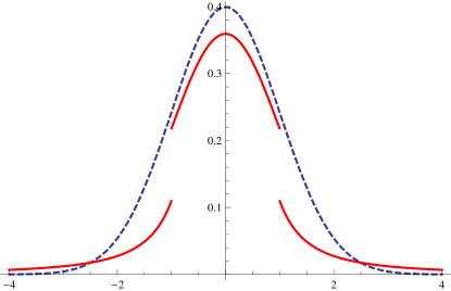
Figure 1: Dotted curve is the normal density function, while solid line is the density of the proposed IS density.

The following Assumption is important for coming up with the parameters of the proposed IS density.

Assumption 1.

There exist $\alpha_{0}>1$ and $\gamma\geq 1$ such that

$$\int_{u\in\Re^{d}}|u|^{\alpha_{0}}\left|\varphi(u)\right|^{\gamma}\,du<\infty\,\,.$$

By Riemann-Lebesgue lemma, if the probability distribution of $X_{1}$ is given by a density function, then $|\varphi(u)|\rightarrow 0$ as $|u|\rightarrow\infty$. Assumption 1 is easily seen to hold when $|\varphi(u)|$ decays as a power law as $|u|\rightarrow\infty$. This is true, for example, for Gamma distributed random variables. More generally, this holds when the underlying density has integrable higher derivatives (see [14]): If $k$-th order derivative of the underlying density is integrable then for any $\alpha_{0}$, Assumption 1 holds with $\gamma>\frac{1+\alpha_{0}}{k}$.

To specify the parameters of the IS density we need further analysis.

Define

$$\varphi_{\theta}(u):=E_{\theta}\left[e^{\iota u\cdot(X_{1}-x_{0})}\right]=e^{-\iota u\cdot x_{0}}\frac{M\left(\theta+\iota u\right)}{M(\theta)}\,\,,$$

where $E_{\theta}$ denotes the expectation operator under the distribution $F_{\theta}$. Let

$$h(x):=1-\sup_{|u|\geq x}|\varphi_{\theta^{*}}(u)|^{2}.$$ (14)

Then $0\leq h(x)\leq 1$, $h(0)=0$, $h(x)$ is continuous, non-decreasing and $h(x)\uparrow 1$ as $x\downarrow 0$. Further, since $\varphi$ is the characteristic function of a non-lattice distribution, $h(x)>0$ if $x>0$. We define

$$h_{1}(y)=\min\{z\,|\,h(z)\geq y\}\,\,\text{for}\,\,y\in(0,1).$$

Then for any $y\in(0,1)$ we have $h(h_{1}(y))\geq y$ and $h_{1}(z)\downarrow 0$ as $z\downarrow 0$.

Let $\{s_{n}\}_{n=1}^{\infty}$ be any sequence with following three properties:

1. $s_{n}\downarrow 0$ as $n\rightarrow\infty$

2. For any $\beta$ positive, $(1-s_{n})^{n}n^{\beta}\rightarrow 0$ as $n\rightarrow\infty$

3. $\sqrt{n}h_{1}(s_{n})\rightarrow\infty$ as $n\rightarrow\infty$

Later in Section 5 we discuss how such a sequence may be selected in practice. Set $\delta_{3}(n):=h_{1}(s_{n})$. Then, it follows that if $x\geq\delta_{3}(n)$ then $h(x)\geq s_{n}$. Equivalently, $|\varphi_{\theta^{*}}(u)|<\sqrt{1-s_{n}}$ for all $u\geq\delta_{3}(n)$.

Let $\kappa_{min}$ and $\kappa_{max}$ denote the minimum and maximum eigenvalue of $\Lambda^{\prime\prime}(\theta^{*})$, respectively. Hence $\frac{1}{\kappa_{min}}$ is the maximum eigenvalue of $\Lambda^{\prime\prime}(\theta^{*})^{-1}=A(\theta^{*})A(\theta^{*})$. Therefore, we have

$$\frac{1}{\kappa_{min}}=||A(\theta^{*})||^{2}\,.$$

Next, put $\delta_{2}(n)=\sqrt{\kappa_{max}}\delta_{3}(n)$. Then, $\sqrt{n}\delta_{2}(n)\rightarrow\infty$ and $|v|\geq\delta_{2}(n)$ implies $|A(\theta^{*})v|\geq\delta_{3}(n)$. Also let

$$\delta_{1}(n)=\frac{1}{\sqrt{\kappa_{min}}}\delta_{2}(n)=\sqrt{\frac{\kappa_{max}}{\kappa_{min}}}\delta_{3}(n),$$

so that $|v|<\delta_{2}(n)$ implies $|A(\theta^{*})v|<\delta_{1}(n)$.

Now we are in position to specify the parameters for the proposed IS density. Set

$$\alpha=\alpha_{0}$$

and

$$a_{n}=\sqrt{n}\delta_{2}(n).$$

Let $p_{n}=b_{n}\times IG\left(\frac{d}{2},\frac{a_{n}^{2}}{2}\right)$. For $g$ to be a valid density function, we need $p_{n}<1$. Since $IG\left(\frac{d}{2},\frac{a_{n}^{2}}{2}\right)\rightarrow 1$, select $b_{n}$ to be a sequence of positive real numbers that converge to 1 in such a way that $b_{n}<1/IG\left(\frac{d}{2},\frac{a_{n}^{2}}{2}\right)$ and

$$\lim_{n\rightarrow\infty}\frac{(1-s_{n})^{n}n^{\frac{d+\alpha}{2}}}{\left[1-b_{n}\times IG\left(\frac{d}{2},\frac{a_{n}^{2}}{2}\right)\right]}=0.$$ (15)

For example, $b_{n}=1-n^{-\xi}$ for any $\xi>0$ satisfies (15). For each $n$, let $g_{n}$ denote the pdf of the form (13) with parameters $\alpha$, $a_{n}$ and $b_{n}$ chosen as above. Let $E_{n}$ and $Var_{n}$ denote the expectation and variance, respectively, w.r.t. the density $g_{n}$.

Theorem 1.

Suppose Assumption 1 holds and $\theta^{*}\in\Theta^{0}$. Then,

$$E_{n}\left[\frac{\psi^{2}(n^{-\frac{1}{2}}A(\theta^{*})V,\theta^{*},n)\phi^{2}(V)}{g^{2}_{n}(V)}\right]=\int_{v\in\Re^{d}}\frac{\psi^{2}(n^{-\frac{1}{2}}A(\theta^{*})v,\theta^{*},n)\phi^{2}(v)}{g_{n}(v)}\,dv=1+o(n^{-\frac{1}{2}})\,.$$

Consequently, from Proposition 2, it follows that

$$Var_{n}\left[\frac{\psi(n^{-\frac{1}{2}}A(\theta^{*})V_{i},\theta^{*},n)\phi(V_{i})}{g_{n}(V_{i})}\right]\rightarrow 0\,\,\,\text{as}\,\,n\rightarrow\infty\,,$$

so that the proposed estimators for $(f_{n}(x_{0}):n\geq 1)$ have an asymptotically vanishing relative error.

We will use the following lemma from [14].

Lemma 1.

For any $\lambda,\,\beta\in\mathbb{C}$,

$$|\exp(\lambda)-1-\beta|\leq\left(|\lambda-\beta|+\frac{|\beta|^{2}}{2}\right)\exp(\omega)\,\,\,\,\text{for all}\,\,\omega\geq\max\{|\lambda|,|\beta|\}\,.$$

Also note that from the definitions of $\psi$ and $\eta$ it follows that, for any $\theta\in\Theta$,

$$\exp\left\{-\frac{v\cdot v}{2}\right\}\psi(n^{-\frac{1}{2}}A(\theta)v,\theta,n)$$

is a characteristic function. To see this, observe that

$$\exp\left\{-\frac{v\cdot v}{2}\right\}\psi(n^{-\frac{1}{2}}A(\theta)v,\theta,n) = \left[\exp\left\{-\frac{v\cdot v}{2n}+\eta\left(n^{-\frac{1}{2}}A(\theta)v,\theta\right)\right\}\right]^{n}$$

$$= \left(E_{\theta}\left[e^{\iota n^{-\frac{1}{2}}A(\theta)v\cdot(X_{1}-x_{0})}\right]\right)^{n}$$

$$= \left[\varphi_{\theta}\left(n^{-\frac{1}{2}}A(\theta)v\right)\right]^{n}.$$

Some more observations are useful for proving Theorem 1.

Since $\eta^{\prime\prime\prime}$ is continuous, it follows from the three term Taylor series expansion,

$$\eta(v,\theta)=\eta(0,\theta)+\eta^{\prime}(0,\theta)v+\frac{1}{2}(v)^{T}\eta^{\prime\prime}(0,\theta)v+\frac{1}{6}\eta^{\prime\prime\prime}(\tilde{v},\theta)\odot v$$

(where $\tilde{v}$ is between $v$ and the origin) and (10) and (11) above that there exists a sequence $\{\epsilon_{n}\}$ of positive numbers converging to zero so that

$$|\eta(v,\theta^{*})-\frac{1}{3!}\eta^{\prime\prime\prime}(0,\theta^{*})\odot v|\leq\epsilon_{n}(\kappa_{min})^{\frac{3}{2}}|v|^{3}\,\,\,\,\text{for}\,\,|v|<\delta_{1}(n),$$

or equivalently

$$|\eta(v,\theta^{*})-\frac{1}{3!}\Lambda^{\prime\prime\prime}(\theta^{*})\odot(\iota v)|\leq\epsilon_{n}(\kappa_{min})^{\frac{3}{2}}|v|^{3}\,\,\,\,\text{for}\,\,|v|<\delta_{1}(n)\,.$$ (16)

Furthermore, for $n$ sufficiently large,

$$\left|\frac{1}{3!}\Lambda^{\prime\prime\prime}(\theta^{*})\odot(\iota v)\right|<\frac{1}{8}\kappa_{min}|v|^{2}$$ (17)

and

$$|\eta(v,\theta^{*})|<\frac{1}{8}\kappa_{min}|v|^{2}$$ (18)

for all $|v|<\delta_{1}(n)$. We shall assume that $n$ is sufficiently large so that (17) and (18) hold in the remaining analysis.

Proof.

( Theorem 1)
We write

$$\int_{v\in\Re^{d}}\frac{\psi^{2}(n^{-\frac{1}{2}}A(\theta^{*})v,\theta^{*},n)\phi^{2}(v)}{g_{n}(v)}\,dv=I_{3}+I_{4}\,.$$

Where

$$I_{3}=\int_{|v|<\sqrt{n}\delta_{2}(n)}\frac{\psi^{2}(n^{-\frac{1}{2}}A(\theta^{*})v,\theta^{*},n)\phi^{2}(v)}{g_{n}(v)}\,dv$$

and

$$I_{4}=\int_{|v|\geq\sqrt{n}\delta_{2}(n)}\frac{\psi^{2}(n^{-\frac{1}{2}}A(\theta^{*})v,\theta^{*},n)\phi^{2}(v)}{g_{n}(v)}\,dv.$$

From (13) we get

$$I_{3}=\frac{1}{b_{n}}\int_{|v|<\sqrt{n}\delta_{2}(n)}\psi^{2}(n^{-\frac{1}{2}}A(\theta^{*})v,\theta^{*},n)\phi(v)\,dv$$

and

$$I_{4}=\frac{1}{C_{n}}\int_{|v|\geq\sqrt{n}\delta_{2}(n)}|v|^{\alpha}\psi^{2}(n^{-\frac{1}{2}}A(\theta^{*})v,\theta^{*},n)\phi^{2}(v)\,dv.$$

For any $c>0$, put

$$\Phi_{d}(c):=\int_{|v|<c}\phi(v)dv\left(=IG\left(\frac{d}{2},\frac{c^{2}}{2}\right)\right)\,.$$

By triangle inequality we have

$$|I_{3}-1|\leq\left|I_{3}-\frac{\Phi_{d}\left(\sqrt{n}\delta_{2}(n)\right)}{b_{n}}\right|+\left|\frac{\Phi_{d}\left(\sqrt{n}\delta_{2}(n)\right)}{b_{n}}-1\right|.$$

Since as $n\rightarrow\infty$ we have $\Phi_{d}\left(\sqrt{n}\delta_{2}(n)\right)\rightarrow 1$ and $b_{n}\rightarrow 1$, the second term in RHS converges to zero. Writing $\zeta_{3}(\theta^{*})=\Lambda^{\prime\prime\prime}(\theta^{*})\star A(\theta^{*})$, for the first term we have

$$\left|I_{3}-\frac{\Phi_{d}\left(\sqrt{n}\delta_{2}(n)\right)}{b_{n}}\right| = \frac{1}{b_{n}}\left|\int_{|v|<\sqrt{n}\delta_{2}(n)}\left\{\psi^{2}(n^{-\frac{1}{2}}A(\theta^{*})v,\theta^{*},n)-1\right\}\phi(v)\,dv\right|$$

$$= \frac{1}{b_{n}}\left|\int_{|v|<\sqrt{n}\delta_{2}(n)}\left\{\psi^{2}(n^{-\frac{1}{2}}A(\theta^{*})v,\theta^{*},n)-1-\frac{\zeta_{3}(\theta^{*})}{3\sqrt{n}}\odot(\iota v)\right\}\phi(v)\,dv\right|$$

$$\leq \frac{1}{b_{n}}\frac{1}{(2\pi)^{\frac{d}{2}}}\int_{|v|<\sqrt{n}\delta_{2}(n)}\left|\psi^{2}(n^{-\frac{1}{2}}A(\theta^{*})v,\theta^{*},n)-1-\frac{\zeta_{3}(\theta^{*})}{3\sqrt{n}}\odot(\iota v)\right|e^{-\frac{v^{2}}{2}}\,dv.$$

We apply Lemma (1) with

$$\lambda=2n\times\eta\left(n^{-\frac{1}{2}}A(\theta^{*})v,\theta^{*}\right)\,\,\,\text{and}\,\,\,\beta=n\frac{\Lambda^{\prime\prime\prime}(\theta^{*})}{3}\odot\left(\iota n^{-\frac{1}{2}}A(\theta^{*})v\right).$$

Since $\frac{|\beta|^{2}}{2}=\frac{1}{n}P(v)$, where $P$ is a homogeneous polynomial whose coefficients does not dependent on $n$, and $|v|<\sqrt{n}\delta_{2}(n)$ implies $|n^{-\frac{1}{2}}A(\theta^{*})v|<\delta_{1}(n)$, we have from (18), (17) and (16), respectively

$$|\lambda|=2n\left|\eta\left(n^{-\frac{1}{2}}A(\theta^{*})v,\theta^{*}\right)\right|<2n\frac{1}{8}\kappa_{min}|n^{-\frac{1}{2}}A(\theta^{*})v|^{2}\leq\frac{1}{8}\kappa_{min}||A(\theta^{*})||^{2}|v|^{2}=\frac{|v|^{2}}{4},$$

$$|\beta|=2n\left|\frac{1}{3!}\Lambda^{\prime\prime\prime}(\theta^{*})\odot\left(\iota n^{-\frac{1}{2}}A(\theta^{*})v\right)\right|<2n\frac{1}{8}\kappa_{min}|n^{-\frac{1}{2}}A(\theta^{*})v|^{2}\leq\frac{1}{8}\kappa_{min}||A(\theta^{*})||^{2}|v|^{2}=\frac{|v|^{2}}{4}$$

and

$$|\lambda-\beta|=2n\left|\eta\left(n^{-\frac{1}{2}}A(\theta^{*})v,\theta^{*}\right)-\frac{1}{3!}\Lambda^{\prime\prime\prime}(\theta^{*})\odot\left(\iota n^{-\frac{1}{2}}A(\theta^{*})v\right)\right|<2n\epsilon_{n}(\kappa_{min})^{\frac{3}{2}}|n^{-\frac{1}{2}}A(\theta^{*})v|^{3}\leq\frac{2\epsilon_{n}|v|^{3}}{\sqrt{n}}.$$

From Lemma 1, it now follows that the integrand in the last integral is dominated by

$$\exp\left\{\frac{|v|^{2}}{4}\right\}\times\left(\frac{2\epsilon_{n}|v|^{3}}{\sqrt{n}}+\frac{1}{n}P(v)\right)\exp\left\{-\frac{|v|^{2}}{2}\right\}\times=\exp\left\{-\frac{|v|^{2}}{4}\right\}\left(\frac{2\epsilon_{n}|v|^{3}}{\sqrt{n}}+\frac{1}{n}P(v)\right).$$

Therefore we have $I_{3}=1+o(n^{-\frac{1}{2}})$.

Also

$$|I_{4}| \leq \frac{1}{(2\pi)^{d}C_{n}}\int_{|v|>\sqrt{n}\delta_{2}(n)}|v|^{\alpha}\left|\exp\left\{-|v|^{2}\right\}\psi^{2}(n^{-\frac{1}{2}}A(\theta^{*})v,\theta^{*},n)\right|\,dv$$

$$= \frac{1}{(2\pi)^{d}C_{n}}\int_{|v|>\sqrt{n}\delta_{2}(n)}|v|^{\alpha}\left|\varphi_{\theta^{*}}\left(n^{-\frac{1}{2}}A(\theta^{*})v\right)\right|^{2n}\,dv$$

$$\leq \frac{(1-s_{n})^{n-\frac{\gamma}{2}}}{(2\pi)^{d}C_{n}}\int_{v\in\Re}|v|^{\alpha}\left|\varphi_{\theta^{*}}\left(n^{-\frac{1}{2}}A(\theta^{*})v\right)\right|^{\gamma}\,dv$$

$$= \frac{(1-s_{n})^{n-\frac{\gamma}{2}}n^{\frac{d+\alpha}{2}}\sqrt{|\Lambda^{\prime\prime}(\theta^{*})|}}{(2\pi)^{d}C_{n}}\int_{u\in\Re}|A(\theta^{*})^{-1}u|^{\alpha}\left|\varphi_{\theta^{*}}(u)\right|^{\gamma}\,du$$

$$\leq D_{1}\frac{(1-s_{n})^{n-\frac{\gamma}{2}}n^{\frac{d+\alpha}{2}}}{C_{n}}\int_{u\in\Re}|u|^{\alpha}\left|\varphi_{\theta^{*}}(u)\right|^{\gamma}\,du$$

$$\leq D_{1}\frac{(1-s_{n})^{n-\frac{\gamma}{2}}n^{\frac{d+\alpha}{2}}\int_{|v|\geq\sqrt{n}\delta_{2}(n)}\frac{dv}{|v|^{\alpha}}}{(1-p_{n})}\int_{u\in\Re}|u|^{\alpha}\left|\varphi_{\theta^{*}}(u)\right|^{\gamma}\,du\,.$$

where $D_{1}$ is a constant independent of $n$. By Assumption 1, the above integral over $u$ is finite. For large $n$ we also have

$$\int_{|v|\geq\sqrt{n}\delta_{2}(n)}\frac{dv}{|v|^{\alpha}}\leq\int_{|v|\geq 1}\frac{dv}{|v|^{\alpha}}.$$

By choice of $b_{n}$ we can conclude that $I_{4}\rightarrow 0$ as $n\rightarrow\infty$, proving Theorem 1. ∎

4 Efficient Estimation of Tail Probability

In this section we consider the problem of efficient estimation of $P(\bar{X}_{n}\in\mathcal{A})$ for sets $\mathcal{A}$ that are affine transformations of the non-negative orthants $\Re^{d}_{+}$ along with some minor variations. As in ([6]), dominating point of the set $\mathcal{A}$ plays a crucial role in our analysis. As is well known, a point $x_{0}$ is called a dominating point of $\mathcal{A}$ if $x_{0}$ uniquely satisfies the following properties (see e.g, [22], [6]):

1. $x_{0}$ is in the boundary of $\mathcal{A}$.

2. There exists a unique $\theta^{*}\in\Re^{d}$ with $\Lambda^{\prime}(\theta^{*})=x_{0}$.

3. $\mathcal{A}\subseteq\{x|\theta^{*}\cdot(x-x_{0})\geq 0\}$.

As is apparent from ([22], [26], [6]), in many cases a general set $\mathcal{A}$ may be partitioned into finitely many sets $(\mathcal{A}_{i}:i\leq m)$ each having its own dominating point. From simulation viewpoint, one way to estimate $P(\bar{X}_{n}\in\mathcal{A})$ then is to estimate each $P(\bar{X}_{n}\in\mathcal{A}_{i})$ separately with an appropriate algorithm. In the remaining paper, we assume the existence of a dominating point $x_{0}$ for $\mathcal{A}$.

Our estimation relies on a saddle-point representation of $P(\bar{X}_{n}\in\mathcal{A})$ obtained using Parseval’s relation. Let

$$Y_{n}:=\sqrt{n}(\bar{X}_{n}-x_{0})$$

and

$$\mathcal{A}_{n,x_{0}}:=\sqrt{n}(\mathcal{A}-x_{0})$$

where $x_{0}=(x_{0}^{1},x_{0}^{2},\ldots,x_{0}^{d})$ is an arbitrarily chosen point in $\Re^{d}$. Let $h_{n,\theta,x_{0}}(y)$ be the density function of $Y_{n}$ when each $X_{i}$ has distribution function $F_{\theta}$, where, recall that

$$dF_{\theta}(x)=\exp(\theta\cdot x)M(\theta)^{-1}dF(x)=\exp\{\theta\cdot x-\Lambda(\theta)\}dF(x)\,.$$

An exact expression for the tail probability is given by:

$$P[\bar{X}_{n}\in\mathcal{A}]=P[Y_{n}\in\mathcal{A}_{n,x_{0}}]=e^{-n\{\theta\cdot x_{0}-\Lambda(\theta)\}}\int_{y\in\mathcal{A}_{n,x_{0}}}e^{-\sqrt{n}(\theta\cdot y)}h_{n,\theta,x_{0}}(y)\,dy\,$$ (19)

which holds for any $\theta\in\Theta$ and any $x_{0}\in\Re^{d}$. The representation (19) is not very useful without further restriction on $x_{0}$ and $\theta$ (see e.g., [22]). Again, assuming that a solution $\theta^{*}\in\Theta^{0}$ to $\Lambda^{\prime}(\theta)=x_{0}$ exists, where $x_{0}$ is the dominating point of $\mathcal{A}$, define

$$c(n,\theta^{*},x_{0})=\int_{y\in\mathcal{A}_{n,x_{0}}}\exp\{-\sqrt{n}(\theta^{*}\cdot y)\}\,dy=n^{\frac{d}{2}}\int_{w\in(\mathcal{A}-x_{0})}\exp\{-n(\theta^{*}\cdot w)\}\,dw$$

We need the following assumption:

Assumption 2.

$\forall n$, $c(n,\theta^{*},x_{0})<\infty$.

Since $x_{0}$ is a dominating point of $\mathcal{A}$, for any $y\in\mathcal{A}_{n,x_{0}}$, we have $\theta^{*}\cdot y\geq 0$. Hence, if $\mathcal{A}$ is a set with finite Lebesgue measure then $c(n,\theta^{*},x_{0})$ is finite. Assumption 2 may hold even when $\mathcal{A}$ has infinite Lebesgue measure, as Example 1 below illustrates.

When Assumption 2 holds, we can rewrite the right hand side of (19) as

$$c(n,\theta^{*},x_{0})e^{-n\{\theta^{*}\cdot x_{0}-\Lambda(\theta^{*})\}}\int_{y\in\mathcal{A}_{n,x_{0}}}r_{n,\theta^{*},x_{0}}(y)h_{n,\theta^{*},x_{0}}(y)\,dy\,$$ (20)

where

$$r_{n,\theta^{*},x_{0}}(y)=\left\{\begin{array}[]{lr}\frac{\exp\{-\sqrt{n}(\theta^{*}\cdot y)\}}{c(n,\theta^{*},x_{0})}&\text{when}\,\,y\in\mathcal{A}_{n,x_{0}}\\ 0&\text{otherwise}\end{array}\right.$$ (21)

is a density in $\Re^{d}$.

Let $\rho_{n,\theta^{*},x_{0}}(t)$ denote the complex conjugate of the characteristic function of $r_{n,\theta^{*},x_{0}}(y)$. Since the characteristic function of $h(n,\theta^{*},x_{0})$ equals

$$e^{-\iota t\sqrt{n}x_{0}}\left[\frac{M\left(\theta^{*}+\frac{\iota t}{\sqrt{n}}\right)}{M(\theta^{*})}\right]^{n},$$

by Parseval’s relation, (20) is equal to

$$c(n,\theta^{*},x_{0})e^{-n\{\theta^{*}\cdot x_{0}-\Lambda(\theta^{*})\}}\left(\frac{1}{2\pi}\right)^{d}\int_{t\in\Re^{d}}\rho_{n,\theta^{*},x_{0}}(t)e^{-\iota t\sqrt{n}x_{0}}\left[\frac{M\left(\theta^{*}+\frac{\iota t}{\sqrt{n}}\right)}{M(\theta^{*})}\right]^{n}\,dt.$$ (22)

This in turn, by the change of variable $t=A(\theta^{*})v$ and rearrangement of terms, equals

$$\frac{c(n,\theta^{*},x_{0})e^{-n\{\theta^{*}\cdot x_{0}-\Lambda(\theta^{*})\}}}{\sqrt{\operatorname{det}(\Lambda^{\prime\prime}(\theta^{*}))}}\left(\frac{1}{2\pi}\right)^{\frac{d}{2}}\int_{v\in\Re^{d}}\rho_{n,\theta^{*},x_{0}}(A(\theta^{*})v)\psi(n^{-\frac{1}{2}}A(\theta^{*})v,\theta^{*},n)\phi(v)\,dv.$$ (23)

We need another assumption to facilitate analysis:

Assumption 3.

For all $t\in\Re^{d}$,

$$\lim_{n\rightarrow\infty}\rho_{n,\theta^{*},x_{0}}(t)=1.$$

Proposition 3.

Suppose $\mathcal{A}$ has a dominating point $x_{0}$, the associated $\theta^{*}\in\Theta^{o}$ and $\Lambda^{\prime\prime}(\theta^{*})$ is strictly positive definite. Further, Assumptions 2 and 3 hold. Then,

$$P[\bar{X}_{n}\in\mathcal{A}]\sim\left(\frac{1}{2\pi}\right)^{\frac{d}{2}}\frac{c(n,\theta^{*},x_{0})e^{-n\{\theta^{*}\cdot x_{0}-\Lambda(\theta^{*})\}}}{\sqrt{\operatorname{det}(\Lambda^{\prime\prime}(\theta^{*}))}},$$ (24)

or, equivalently by (23)

$$\lim_{n\rightarrow\infty}\int_{v\in\Re^{d}}\rho_{n,\theta^{*},x_{0}}(A(\theta^{*})v)\psi(n^{-\frac{1}{2}}A(\theta^{*})v,\theta^{*},n)\phi(v)\,dv=1.$$ (25)

Proof of Proposition 3 is omitted. It follows along the line of proof of Proposition 2 and from noting that:

$$\lim_{n\rightarrow\infty}\int_{v\in\Re^{d}}\rho_{n,\theta^{*},x_{0}}(A(\theta^{*})v)\phi(v)\,dv=1,$$

$$\lim_{n\rightarrow\infty}\int_{v\in\Re^{d}}v_{i}v_{j}v_{k}\rho_{n,\theta^{*},x_{0}}(A(\theta^{*})v)\phi(v)\,dv=0.$$

Let $g$ be any density supported on $\Re^{d}$. If $V_{1},V_{2},\ldots,V_{N}$ are iid with distribution given by density $g$, then the unbiased estimator for $P[\bar{X}_{n}\in\mathcal{A}]$ is given by

$$\hat{P}[\bar{X}_{n}\in\mathcal{A}] = \left(\frac{1}{2\pi}\right)^{\frac{d}{2}}\frac{c(n,\theta^{*},x_{0})e^{-n\{\theta^{*}\cdot x_{0}-\Lambda(\theta^{*})\}}}{\sqrt{\operatorname{det}(\Lambda^{\prime\prime}(\theta^{*}))}}$$ (26)

$$\times\frac{1}{N}\sum_{j=1}^{N}\frac{\rho_{n,\theta^{*},x_{0}}(A(\theta^{*})V_{j})\psi(n^{-\frac{1}{2}}A(\theta^{*})V_{j},\theta^{*},n)\phi(V_{j})}{g(V_{j})}.$$

Note that for above estimator to be useful, one must be able to find closed form expression for $c(n,\theta^{*},x_{0})$ and $\rho_{n,\theta^{*},x_{0}}(t)$ or these should be cheaply computable. In Section 4.1, we consider some examples where we explicitly compute $c(n,\theta^{*},x_{0})$ and $\rho_{n,\theta^{*},x_{0}}$ and verify Assumptions 2 and 3.

Theorem 2.

Under Assumptions 1, 2 and 3,

$$E_{n}\left[\frac{\rho_{n,\theta^{*},x_{0}}^{2}(A(\theta^{*})V)\psi^{2}(n^{-\frac{1}{2}}A(\theta^{*})V,\theta^{*},n)\phi^{2}(V)}{g_{n}^{2}(V)}\right]=1+o(n^{-\frac{1}{2}})\,\,\,\,\text{as}\,\,\,n\rightarrow\infty,$$

where $g_{n}$ is same as Theorem 1. Consequently, by Proposition 3, it follows that as $n\rightarrow\infty$

$$Var_{n}\left[\hat{P}[\bar{X}_{n}\in\mathcal{A}]\right]\rightarrow 0$$

and the proposed estimator has asymptotically vanishing relative error.

The proof of Theorem 2 is given in the appendix.

4.1 Examples

Example 1.

Let $\mathcal{A}=x_{0}+{\Re_{+}^{d}}$, where $x_{0}=(x_{0}^{1},x_{0}^{2},\ldots,x_{0}^{d})$ is a given point in $\Re^{d}$. Further suppose that $\forall i=1,2,\ldots,d,\,\,\theta_{i}^{*}>0$. It is easy to see that existence of such a $\theta^{*}$ implies that $x_{0}$ is a dominating point for $\mathcal{A}$. It also follows that Assumption 2 holds and

$$c(n,\theta^{*},x_{0})=\frac{1}{n^{\frac{d}{2}}\theta_{1}^{*}\theta_{2}^{*}\cdots\theta_{d}^{*}}.$$

It can easily be verified that

$$\rho_{n,\theta^{*},x_{0}}(t_{1},t_{2},\ldots t_{d})=\prod_{i=1}^{d}\left(\frac{1}{1+\frac{\iota t_{i}}{\sqrt{n}\theta_{i}^{*}}}\right).$$

Therefore Assumption 3 also holds in this case. By Proposition 3, we then have

$$P[\bar{X}_{n}-x_{0}\in\Re_{+}^{d}]\sim\frac{e^{n\left\{\Lambda(\theta^{*})-\theta^{*}\cdot x_{0}\right\}}}{(2\pi)^{\frac{d}{2}}n^{\frac{d}{2}}\sqrt{\operatorname{det}(\Lambda^{\prime\prime}(\theta^{*}))}\theta_{1}^{*}\theta_{2}^{*}\cdots\theta_{d}^{*}}.$$

By Theorem 2,

$$\hat{P}[\bar{X}_{n}-x_{0}\in\Re_{+}^{d}]:=\frac{e^{n\left\{\Lambda(\theta^{*})-\theta^{*}\cdot x_{0}\right\}}}{(2\pi)^{\frac{d}{2}}n^{\frac{d}{2}}\sqrt{\operatorname{det}(\Lambda^{\prime\prime}(\theta^{*}))}\theta_{1}^{*}\theta_{2}^{*}\cdots\theta_{d}^{*}}\times\frac{1}{N}\sum_{j=1}^{N}\frac{\psi(n^{-\frac{1}{2}}A(\theta^{*})V_{j},\theta^{*},n)\phi(V_{j})}{\prod_{i=1}^{d}\left(1+\frac{\iota e_{i}^{T}A(\theta^{*})V_{j}}{\sqrt{n}\theta_{i}^{*}}\right)g(V_{j})}$$ (27)

is an unbiased estimator for $P[\bar{X}_{n}-x_{0}\in\Re_{+}^{d}]$ and has an asymptotically vanishing relative error.

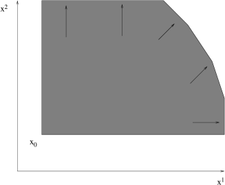
(a) $\mathcal{A}=x_{0}+\Re_{+}^{d}$.

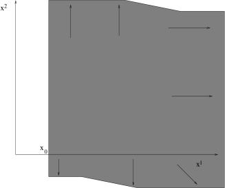
(b) $\mathcal{A}=x_{0}+Q_{1}^{+}$ .

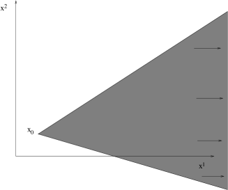
(c) $\mathcal{A}=x_{0}+B{\Re_{+}^{d}}$.

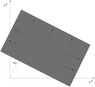
(d) $\mathcal{A}=x_{0}+BQ_{1}^{+}$.

Figure 2: $\mathcal{A}$ is shown as shaded region ($d=2$).

Example 2.

For $0\leq d^{\prime}\leq d$, let

$$Q_{d^{\prime}}^{+}:=\{(x_{1},x_{2},\ldots,x_{d})\in\Re^{d}|\,\,x_{i}\geq 0\,\,\,\forall\,\,\,0\leq i\leq d^{\prime}\}.$$

Suppose we want to estimate $P[\bar{X}_{n}\in\mathcal{A}]$, where, now $\mathcal{A}=x_{0}+Q_{d^{\prime}}^{+}$ and $x_{0}$ is a given point in $\Re^{d}$ (see Figure 2(b)). We proceed as in Example 1. In this case Equation (19) is

$$P[\bar{X}_{n}\in\mathcal{A}]=e^{-n\{\theta\cdot x_{0}-\Lambda(\theta)\}}\int_{y\in Q_{d^{\prime}}^{+}}e^{-\sqrt{n}(\theta\cdot y)}h_{n,\theta,x_{0}}(y)\,dy$$ (28)

We now assume that $\theta^{*}_{i}>0,\,\,\forall i\leq d^{\prime}$ and $\theta^{*}_{i}=0\,\,\forall i>d^{\prime}$

Dividing the right hand side of equation (28) by $\sqrt{n}\theta^{*}_{1},\sqrt{n}\theta^{*}_{2},\ldots,\sqrt{n}\theta^{*}_{d^{\prime}}$ s and integrating out $y_{d^{\prime}+1},y_{d^{\prime}+2},\ldots,y_{d}$ we obtain

$$\frac{e^{n\left\{\Lambda(\theta^{*})-\theta^{*}\cdot x_{0}\right\}}}{n^{\frac{d^{\prime}}{2}}\theta^{*}_{1}\theta^{*}_{2}\cdots\theta^{*}_{d^{\prime}}}\int_{y_{i}>0\forall i\leq d^{\prime}}\left(\prod_{i=1}^{d^{\prime}}\sqrt{n}\theta^{*}_{i}e^{-\sqrt{n}\theta^{*}_{i}y_{i}}\right)\left(\int_{y_{i}\in\mathbb{R}\forall d^{\prime}<i\leq d}h_{n,\theta^{*},x_{0}}(y)\prod_{i=d^{\prime}+1}^{d}dy_{i}\right)\prod_{i=1}^{d^{\prime}}dy_{i},$$

which we can write as

$$\frac{e^{n\left\{\Lambda(\theta^{*})-\theta^{*}\cdot x_{0}\right\}}}{n^{\frac{d^{\prime}}{2}}\theta^{*}_{1}\theta^{*}_{2}\cdots\theta^{*}_{d^{\prime}}}\int_{y_{i}>0\forall i\leq d^{\prime}}\left(\prod_{i=1}^{d^{\prime}}\sqrt{n}\theta^{*}_{i}e^{-\sqrt{n}\theta^{*}_{i}y_{i}}\right)\tilde{h}_{n,\theta^{*},x_{0}}(y_{1},y_{2},\ldots,y_{d^{\prime}})\prod_{i=1}^{d^{\prime}}dy_{i},$$

where $\tilde{h}_{n,\theta^{*},x_{0}}(y_{1},y_{2},\ldots,y_{d^{\prime}})$ is the density function of $(Y^{1},Y^{2},\ldots,Y^{d^{\prime}})$ under the measure induced by $F_{\theta^{*}}$. Thus, the problem reduces to that in Example 1 with dimension $d^{\prime}$ instead of $d$. In this case,

$$c(n,\theta^{*},x_{0})=\frac{1}{n^{\frac{d^{\prime}}{2}}\theta^{*}_{1}\theta^{*}_{2}\cdots\theta^{*}_{d^{\prime}}}$$

and

$$\rho(n,\theta^{*},x_{0})(t_{1},t_{2},\ldots t_{d})=\prod_{i=1}^{d^{\prime}}\left(\frac{1}{1+\frac{\iota t_{i}}{\sqrt{n}\theta^{*}_{i}}}\right).$$

Thus, both the Assumptions 2 and 3 hold and we have

$$P[\bar{X}_{n}\in\mathcal{A}]\sim\frac{e^{n\left\{\Lambda(\theta^{*})-\theta^{*}\cdot x_{0}\right\}}}{(2\pi n)^{\frac{d^{\prime}}{2}}\sqrt{\operatorname{det}(\Lambda^{\prime\prime}(\theta^{*}))}\theta^{*}_{1}\theta^{*}_{2}\cdots\theta^{*}_{d^{\prime}}}.$$

Furthermore, the associated estimator has an asymptotically vanishing relative error.

Example 3.

When $\mathcal{A}=x_{0}+B{\Re_{+}^{d}}$ and $B$ a nonsingular matrix (see Figure 2(c)), the problem can also be reduced to that considered in Example 1 by a simple change of variable. Set $y=B^{-1}z$. Then, it follows that for any $\theta$

$$c(n,\theta,x_{0})=\text{det}(B)\int_{z\in\Re_{+}^{d}}\exp\{-\sqrt{n}(B^{T}\theta\cdot z)\}\,dz.$$

Now if we assume that all the $d$ components of $B^{T}\theta^{*}$ are positive, then as in Example 1, both the Assumptions 2 and 3 hold.

Similar analysis holds when $\mathcal{A}=x_{0}+B{Q_{d^{\prime}}^{+}}$, $(1\leq d^{\prime}<d)$, and $B$ a nonsingular matrix. Then, simple change of variable $y=B^{-1}z$ reduces the problem to that in Example 2.

(a)

(b)

Figure 3: Set $\mathcal{A}^{(i)}$ is the region labeled $i$ ($i=1,2,3$, $\mathcal{A}^{(1)}\subset\mathcal{A}^{(2)}\subset\mathcal{A}^{(3)}$.)

Example 4.

In above examples we have considered sets $\mathcal{A}$ which are unbounded. In this example we show that similar analysis holds when the set $\mathcal{A}$ is bounded. Consider the three increasing regions $(\mathcal{A}_{i}:i=1,2,3)$ as depicted in Figure 3(a). Here $\mathcal{A}_{3}$ corresponds to region $\mathcal{A}$ considered in Example 1. $x_{0}$ is the common dominating point for all the three sets. Again suppose that $\forall i=1,2,\ldots,d,\,\,\theta_{i}^{*}>0$. Suppressing dependence on $x_{0}$ and $\theta^{*}$, for $i=1,2$, let

$$c_{n}^{(i)}:=\int_{y\in\sqrt{n}(\mathcal{A}^{(i)}-x_{0})}\exp\{-\sqrt{n}(\theta^{*}\cdot y)\}\,dy$$

and

$$\rho_{n}^{(i)}(t):=\frac{1}{c_{n}^{(i)}}\int_{y\in\sqrt{n}(\mathcal{A}^{(i)}-x_{0})}\exp\{-\iota t\cdot y-\sqrt{n}(\theta^{*}\cdot y)\}\,dy.$$

If $\mathcal{A}^{(1)}$ is the $d$-dimensional rectangle given by $\prod_{i}^{d}[x_{0}^{i},x_{0}^{i}+D_{i}]$ then

$$c_{n}^{(1)}=\frac{(1-e^{-n\theta_{1}^{*}D_{1}})(1-e^{-n\theta_{2}^{*}D_{2}})\cdots(1-e^{-n\theta_{d}^{*}D_{d}})}{n^{\frac{d}{2}}\theta_{1}^{*}\theta_{2}^{*}\cdots\theta_{d}^{*}}$$

and

$$\rho_{n}^{(1)}(t_{1},t_{2},\ldots t_{d})=\prod_{i=1}^{d}\left(\frac{1}{1+\frac{\iota t_{i}}{\sqrt{n}\theta_{i}^{*}}}\times\frac{1-e^{-n\theta_{i}^{*}D_{i}(1+\frac{\iota t_{i}}{\sqrt{n}\theta_{i}^{*}})}}{1-e^{-n\theta_{i}^{*}D_{i}}}\right).$$

Therefore, it follows that Assumption 3 holds for $\mathcal{A}^{(1)}$. Also note that,

$$|\rho_{n}^{(2)}(t)-1| \leq \frac{1}{c_{n}^{(2)}}\int_{y\in\sqrt{n}(\mathcal{A}^{(2)}-x_{0})}\exp\{-\sqrt{n}(\theta^{*}\cdot y)\}\left|e^{-\iota t\cdot y}-1\right|\,dy$$

$$\leq \frac{1}{n^{\frac{d}{2}}c_{n}^{(1)}}\int_{z\in n(\mathcal{A}^{(2)}-x_{0})}\exp\{-\theta^{*}\cdot z\}\left|e^{-\frac{\iota t\cdot z}{\sqrt{n}}}-1\right|\,dz$$

$$\leq \frac{1}{n^{\frac{d}{2}}c_{n}^{(1)}}\int_{z\in\Re_{+}^{d}}\exp\{-\theta^{*}\cdot z\}\left|e^{-\frac{\iota t\cdot z}{\sqrt{n}}}-1\right|\,dz.$$

Since the last integral converges to zero, it follows that Assumption 3 holds for $\mathcal{A}^{(2)}$. Similar analysis carries over to sets as illustrated by Figure 3(b) under the conditions as in Example 3.

In Example 1 we assumed that $\forall i=1,2,\ldots,d,\,\,\theta_{i}^{*}>0$. In many setting, this may not be true but the problem can be easily transformed to be amenable to the proposed algorithms. We illustrate this through the following example. Essentially, in many cases where such a $\theta^{*}$ does not exist, the problem can be transformed to a finite collection of subproblems, each of which may then be solved using the proposed methods.

Example 5.

Let $(X_{i}:i\geq 1)$ be a sequence of independent rv’s with distribution same as $X=(Z_{1},Z_{2})$, where $Z_{1}$ and $Z_{2}$ are standard normal rvs with correlation $\rho$. Suppose $\mathcal{A}:=(a,b)+\Re^{2}_{+}$, that is $\mathcal{A}:=\{(z_{1},z_{2})|z_{1}\geq a\,\,\text{and}\,\,z_{2}\geq b\}$. Solving $\Lambda^{\prime}(\theta_{1},\theta_{2})=(a,b)$ we get

$$\theta_{1}^{*}=\frac{a-\rho b}{1-\rho^{2}}\,\,\,\,\text{and}\,\,\,\,\theta_{2}^{*}=\frac{b-\rho a}{1-\rho^{2}}$$

Thus, if $\min\{\frac{a}{b},\frac{b}{a}\}>\rho$ we have both $\theta_{1}^{*}$ and $\theta_{2}^{*}$ positive, and we are in situation of Example 1. Suppose $\frac{b}{a}<\rho$ so that $\theta_{2}^{*}<0$. Then making the change of variable $Z_{3}=-Z_{2}$ we have

$$P[\bar{Z_{1}}\geq a,\bar{Z_{2}}\geq b]=P[\bar{Z_{1}}\geq a]-P[\bar{Z_{1}}\geq a,\bar{Z_{3}}\geq-b].$$

Now for estimating the second probability we have both $\theta_{1}^{*}$ and $\theta_{2}^{*}$ positive. Similarly, the first probability is easily estimated using the proposed algorithm.

However, note that if $(a,b)$ lies on $\{(z_{1},z_{2})|z_{1}=\rho z_{2}\,\,\text{or}\,\,z_{2}=\rho z_{1}\}$ we have one of $\theta_{1}^{*}$ or $\theta_{2}^{*}$ zero, and consequently $c(n,\theta_{1}^{*},\theta_{2}^{*},a,b)$ is infinite. The proposed algorithms may need to be modified to handle such situations, however its not clear if simple adjustment to our algorithm will result in the asymptotically vanishing relative error property. We further discuss restrictions to our approach in Section 6.

4.2 Estimating expected overshoot

The methodology developed previously to estimate the tail probability $P(\bar{X}_{n}\in\mathcal{A})$ can be extended to estimate $E[\bar{X}_{n}^{\alpha}\,|\bar{X}_{n}\in\mathcal{A}]$ for $\alpha\in(\mathbb{Z}_{+}-\{0\})^{d}$. We illustrate this in a single dimension setting ($d=1$) for $\alpha=1$, and $\mathcal{A}=(x_{0},\infty)$ for $x_{0}>EX_{i}$.

Let $S_{n}=\sum_{i=1}^{n}X_{i}$. In finance and in insurance one is often interested in estimating $E[(S_{n}-nx_{0})|S_{n}>nx_{0}]$, which is known as the expected overshoot or the peak over threshold. As we have an efficient estimator for $P(\bar{X}_{n}>x_{0})$, the problem of efficiently estimating $E[S_{n}|S_{n}>nx_{0}]$ is equivalent to that of efficiently estimating $E[(S_{n}-nx_{0})I(S_{n}>nx_{0})]$. Note that

$$E[((S_{n}-nx_{0})I(S_{n}>nx_{0})]=\sqrt{n}E[Y_{n}I(Y_{n}>0)],$$

where $Y_{n}=\sqrt{n}(\bar{X}_{n}-x_{0})$. Using (19) we get

$$E[Y_{n}I(Y_{n}>0)]=e^{-n\{\theta^{*}\cdot x_{0}-\Lambda(\theta^{*})\}}\int_{0}^{\infty}y\,e^{-\sqrt{n}(\theta^{*}\cdot y)}h_{n,\theta^{*},x_{0}}(y)\,dy,$$ (29)

where recall that $\theta^{*}\in\Theta$ is a solution to $\Lambda^{\prime}(\theta)=x_{0}$ and $h_{n,\theta^{*},x_{0}}(y)$ is the density of $Y_{n}$ when each $X_{i}$ has distribution $F_{\theta^{*}}$. Define

$$\tilde{c}(n,\theta^{*})=\int^{\infty}_{0}y\,\exp\{-\sqrt{n}(\theta^{*}\cdot y)\}\,dy=(n\,{\theta^{*}}^{2})^{-1}$$

Hence, $\forall n$, $\tilde{c}(n,\theta^{*})<\infty$. The right hand side of (29) may be re-expressed as

$$\tilde{c}(n,\theta^{*})e^{-n\{\theta^{*}\cdot x_{0}-\Lambda(\theta^{*})\}}\int^{\infty}_{0}\tilde{r}_{n,\theta^{*}}(y)h_{n,\theta^{*},x_{0}}(y)\,dy\,$$ (30)

where,

$$\tilde{r}_{n,\theta^{*}}(y)=\left\{\begin{array}[]{lr}\frac{y\,\exp\{-\sqrt{n}(\theta^{*}\cdot y)\}}{\tilde{c}(n,\theta^{*})}&\text{when}\,\,y>0\\ 0&\text{otherwise}\end{array}\right.$$ (31)

is a density in $\Re_{+}$.

Let $\tilde{\rho}_{n,\theta^{*}}(t)$ denote the complex conjugate of the characteristic function of $\tilde{r}_{n,\theta^{*}}(y)$. By simple calculations, it follows that

$$\tilde{\rho}_{n,\theta^{*}}(t)=\frac{1}{1-\frac{t^{2}}{n{\theta^{*}}^{2}}-\frac{2\iota\,t}{\sqrt{n}\theta^{*}}}\,\,,$$

and $\underset{n\rightarrow\infty}{\lim}\tilde{\rho}_{n,\theta^{*}}(t)=1.$ Then, repeating the analysis for the tail probability, analogously to (23), we see that (30) equals

$$\frac{\tilde{c}(n,\theta^{*})e^{-n\{\theta^{*}\cdot x_{0}-\Lambda(\theta^{*})\}}}{\sqrt{2\pi\,\Lambda^{\prime\prime}(\theta^{*})}}\int^{\infty}_{0}\tilde{\rho}_{n,\theta^{*}}(A(\theta^{*})v)\psi(n^{-\frac{1}{2}}A(\theta^{*})v,\theta^{*},n)\phi(v)\,dv.$$

As in Proposition 3, we can see that

$$E[(S_{n}-nx_{0})I(S_{n}>nx_{0})]\sim\left(\frac{n}{2\pi}\right)^{\frac{1}{2}}\frac{\tilde{c}(n,\theta^{*})e^{-n\{\theta^{*}\cdot x_{0}-\Lambda(\theta^{*})\}}}{\sqrt{\operatorname{det}(\Lambda^{\prime\prime}(\theta^{*}))}}=\left(\frac{1}{2\pi n}\right)^{\frac{1}{2}}\frac{e^{-n\{\theta^{*}\cdot x_{0}-\Lambda(\theta^{*})\}}}{{\theta^{*}}^{2}\sqrt{\operatorname{det}(\Lambda^{\prime\prime}(\theta^{*}))}},$$

so that

$$\frac{E[(S_{n}-nx_{0})I(S_{n}>nx_{0})]}{P[S_{n}>nx_{0}]}\sim\frac{1}{\theta^{*}}.$$

Using analysis identical to that in Theorem 2, it follows that the resulting unbiased estimator of $E[(S_{n}-nx_{0})I(S_{n}>nx_{0})]$ (when density $g_{n}$ is used) has an asymptotically vanishing relative error.

The above analysis can be easily extended to prove similar results for the case of $X_{i}\in\Re^{d}$ and $\alpha$ a vector of positive integers.

5 Numerical Experiments

5.1 Choice of parameters of IS density

To implement the proposed method, the user must first specify the parameters of the IS density $g_{n}$ appropriately. In this subsection we indicate how this may be done in practice. All the user needs is to identify a sequence $\{s_{n}\}_{n=1}^{\infty}$ satisfying the three properties listed in Subsection 3.1.2. Once $\{s_{n}\}_{n=1}^{\infty}$ is specified, arriving at appropriate $\alpha$, $a_{n}$, and $b_{n}$ is straightforward (see discussion before Theorem 1; Finding $A(\theta^{*})$, $\kappa_{max}$ and $\kappa_{min}$ are one time computations and can be efficiently done using MATLAB or MATHEMATICA).

Clearly for any $\epsilon\in(0,1)$, $s_{n}:=\frac{1}{n^{\epsilon}}$ satisfies properties 1 and 2. To see that property 3 also holds, note that

$$1-|\varphi_{\theta^{*}}(t)|^{2}=\int_{x\in\Re^{d}}(1-\cos(t\cdot x))d\tilde{F}_{\theta^{*}}(x),$$

where $\tilde{F}_{\theta^{*}}(x)$ is the symmetrization of $F_{\theta^{*}}(x)$ (if $G$ is the distribution function of random vector $Y$ then symmetrization of $G$, denoted $\tilde{G}$, is the distribution function of the random vector $Y+Z$, where $Z$ has same distribution as $-Y$). Since

$$\frac{(t\cdot x)^{2}}{2!}-\frac{(t\cdot x)^{4}}{4!}\leq 1-\cos(t\cdot x)\leq\frac{(t\cdot x)^{2}}{2!},$$

it follows that there exist a neighborhood $U\subset\Re^{d}$ of origin and positive constants $c$ and $C$, such that

$$c|t|^{2}\leq 1-|\varphi_{\theta^{*}}(t)|^{2}\leq C|t|^{2}$$

for all $t\in U$. This in turn implies that there is a neighborhood $V\subset\Re$ of zero and positive constants $c,C,c_{1}$ and $C_{1}$ such that

$$cx^{2}\leq h(x)\leq Cx^{2}$$

and

$$c_{1}\sqrt{x}\leq h_{1}(x)\leq C_{1}\sqrt{x}$$

for all $x\in V$. Therefore $\sqrt{n}h_{1}(s_{n})=\sqrt{n}h_{1}(n^{-\epsilon})\geq cn^{\frac{1}{2}-\frac{\epsilon}{2}}\rightarrow\infty$ for any $\epsilon<1$.

One may choose $\epsilon$ close to $1$ so that $\sqrt{n}h_{1}(s_{n})$ grows slowly. Then, since $a_{n}=\sqrt{n}\delta_{2}(n)=\sqrt{\kappa_{max}}\sqrt{n}h_{1}(s_{n})$, $a_{n}$ can be taken approximately a constant over a specified range of variation of $n$. Also since $p_{n}=b_{n}\times IG\left(\frac{d}{2},\frac{a_{n}^{2}}{2}\right)$ is what one uses for simulating from $g_{n}$, and $p_{n}\uparrow 1$, in practice for reasonable values of $n$, one may take $p_{n}$ as a constant close to 1. In our numerical experiment below, parameters for $g_{n}$ are chosen using these simple guidelines.

5.2 Estimation of probability density function of $\bar{X}_{n}$

We first use the proposed method to estimate the probability density function of $\bar{X}_{n}$ for the case where sequence of random variables $(X_{i}:i\geq 1)$ are independent and identically exponentially distributed with mean 1. Then the sum has a known gamma density function facilitating comparison of the estimated value to the true value. The density function estimates using the proposed method (referred to as SP-IS method) are evaluated for $n=30$, $a_{n}=2,\alpha=2$ and $p_{n}=0.9$ (the algorithm performance was observed to be relatively insensitive to small perturbations in these values) based on $N$ generated samples. Table 1 shows the comparison of our method with the conditional Monte Carlo (CMC) method proposed in Asmussen and Glynn (2008) (pg. 145-146) for estimating the density function of $\bar{X}_{n}$ at a few values. As discussed in Asmussen and Glynn (2008), the CMC estimates are given by an average of $N$ independent samples of $nf(x-S_{n-1})$, where $S_{n-1}$ is generated by sampling $(X_{1},\ldots,X_{n-1})$ using their original density function $f$. Figure 4 shows this comparison graphically over a wider range of density function values. As may be expected, the proposed method provides an estimator with much smaller variance compared to the CMC method.

$x$	True value	SP-IS	Sample	CMC	Sample
		estimate	variance	estimate	variance
1.0	2.179	2.185	0.431	2.360	31.387
1.5	0.085	0.087	4.946 $\times 10^{-4}$	0.067	0.478
2.0	1.094 $\times 10^{-4}$	$1.105\times 10^{-4}$	$1.066\times 10^{-9}$	$7.342\times 10^{-7}$	$3.341\times 10^{-1}$

Table 1: True density function and its estimates using the proposed (SP-IS) method and the conditional Monte Carlo (CMC) for an average of 30 independent exponentially distributed mean = 1 random variables. For $x=1.0$ and $1.5$, the number of generated samples $N=1000$ in both the methods, and for $x=2.0$, $N=10,000$.

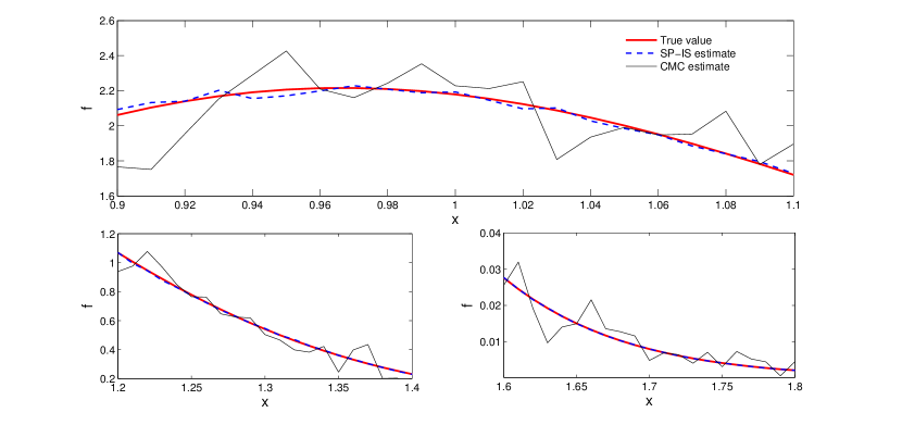
Figure 4: True density function and its estimates using the proposed (SP-IS) method and the conditional Monte Carlo (CMC) for an average of 30 independent exponentially distributed mean = 1 random variables. This plot illustrates the performance of the two methods over wide range of $x$ values. In both simulations $N=1,000$ at each point.

5.3 Comparison with independent exponential twisting approach

We consider a simple numerical experiment in dimension $d=3$ to compare efficiency of the proposed method with the one involving state independent exponential twisting proposed by Sadowsky and Bucklew (1990). We consider a sequence of random vectors $(X_{i},Y_{i},Z_{i}:i\geq 1)$ that are independent and identically distributed as follows: Let $E_{1},E_{2},E_{3}$ be iid exponentially distributed with mean 1. Define rvs $X$, $Y$ and $Z$ as

$$X=\frac{1}{2}\left(E_{1}+E_{2}\right)$$

$$Y=\frac{1}{2}\left(E_{2}+E_{3}\right)$$

$$Z=\frac{1}{2}\left(E_{3}+E_{1}\right)$$

Each $(X_{i},Y_{i},Z_{i})$ for $i=1,2,\ldots,n$ has the same distribution as $(X,Y,Z)$. We estimate the probability $P(\bar{X}_{n}\geq x,\bar{Y}_{n}\geq y,\bar{Z}_{n}\geq z)$ for $x=1.4$, $y=1.5$ and $z=1.4$ and different values of $n$. Table 2 below reports the estimates based on $N$ generated samples. $c_{n}$ denotes the exact asymptotic (the saddle point estimate) corresponding to the probability. These differ substantially from the estimated probability values, emphasizing the inaccuracy of $c_{n}$ even for reasonably large values of $n$, and thus motivating simulation as a tool for accurate estimation of the associated rare probabilities.

In these experiments we set $a_{n}=2$, $\alpha=3$ and $p_{n}=0.95$. We also report the variance reduction achieved by the proposed method over the one proposed by Sadowsky and Bucklew (1990). This is substantial and it increases with increasing $n$.

Table 2: Comparison of the proposed methodology (SP-IS) with optimal state independent exponential twisting (OET). In second and third columns we report the $95\%$ confidence intervals for the tail probability under SP-IS and OET respectively.

n=10			$c_{n}=0.0122562$
N	OET	SP-IS	Variance reduction
1000	$(2.391\pm 0.494)\times 10^{-3}$	$(2.492\pm 0.211)\times 10^{-3}$	$5.48$
10000	$(2.546\pm 0.163)\times 10^{-3}$	$(2.478\pm 0.073)\times 10^{-3}$	$4.98$
100000	$(2.503\pm 0.05)\times 10^{-3}$	$(2.479\pm 0.024)\times 10^{-3}$	$4.34$
n=20			$c_{n}=4.490\times 10^{-4}$
N	OET	SP-IS	Variance reduction
1000	$(1.621\pm 0.373)\times 10^{-4}$	$(1.383\pm 0.102)\times 10^{-4}$	$13.37$
10000	$(1.507\pm 0.118)\times 10^{-4}$	$(1.513\pm 0.029)\times 10^{-4}$	$16.55$
100000	$(1.506\pm 0.037)\times 10^{-4}$	$(1.474\pm 0.009)\times 10^{-4}$	$16.90$
n=40			$c_{n}=1.704\times 10^{-6}$
N	OET	SP-IS	Variance reduction
1000	$(7.349\pm 2.346)\times 10^{-7}$	$(8.309\pm 0.364)\times 10^{-7}$	$41.53$
10000	$(7.77\pm 0.757)\times 10^{-7}$	$(8.186\pm 0.115)\times 10^{-7}$	$43.33$
100000	$(8.039\pm 0.255)\times 10^{-7}$	$(8.181\pm 0.037)\times 10^{-7}$	$47.50$
n=60			$c_{n}=9.960\times 10^{-9}$
N	OET	SP-IS	Variance reduction
1000	$(5.411\pm 2.051)\times 10^{-9}$	$(5.869\pm 0.257)\times 10^{-9}$	$63.69$
10000	$(5.734\pm 0.668)\times 10^{-9}$	$(5.632\pm 0.071)\times 10^{-9}$	$88.52$
100000	$(5.666\pm 0.214)\times 10^{-9}$	$(5.651\pm 0.023)\times 10^{-9}$	$86.57$
n=80			$c_{n}=6.946\times 10^{-11}$
N	OET	SP-IS	Variance reduction
1000	$(4.101\pm 1.664)\times 10^{-11}$	$(4.337\pm 0.181)\times 10^{-11}$	$84.52$
10000	$(4.615\pm 0.622)\times 10^{-11}$	$(4.401\pm 0.059)\times 10^{-11}$	$111.14$
100000	$(4.343\pm 0.187)\times 10^{-11}$	$(4.381\pm 0.018)\times 10^{-11}$	$107.93$
n=100			$c_{n}=5.336\times 10^{-13}$
N	OET	SP-IS	Variance reduction
1000	$(3.676\pm 1.478)\times 10^{-13}$	$(3.618\pm 0.146)\times 10^{-13}$	$102.48$
10000	$(3.923\pm 0.533)\times 10^{-13}$	$(3.637\pm 0.049)\times 10^{-13}$	$118.32$
100000	$(3.546\pm 0.172)\times 10^{-13}$	$(3.609\pm 0.016)\times 10^{-13}$	$115.56$

5.4 Comparison with state dependent exponential twisting

We compare the efficiency of SP-IS method for estimating the tail probability $P(\bar{X}_{n}\in\mathcal{A})$ with the optimal state dependent exponential twisting method proposed by [5] (referred to as BGL method). They restrict their analysis to convex sets $\mathcal{A}$ with twice continuously differentiable boundary whereas SP-IS method is applicable to sets that are affine transformations of the non-negative orthants $\Re^{d}_{+}$. The two methods agree in the single dimension and hence we compare them on a single dimension example.

For a sequence of random variables $(X_{i}:i\geq 1)$ that are independent and identically exponentially distributed with mean 1, $P(\bar{X}_{n}\geq 1.5)$ is estimated for different values of $n$. Table 3 reports the estimates based on different $N$ generated samples. In this experiment, $a_{n}=2,\alpha=2$ and $p_{n}=0.9$ for SP-IS method. BGL method is implemented as per [5] as follows: first $X_{1}$ is generated using an exponentially twisted distribution with mean $x_{0}=1.5$. At each next step, the exponential twisting coefficient in the distribution used to generate $X_{k+1}$ is recomputed such that mean of the distribution is $\frac{nx_{0}-\sum_{i=1}^{k}X_{i}}{n-k}$. The exponential twisting is dynamically updated until the generated $\sum_{i=1}^{k}X_{i}\geq nx_{0}$ at which point we stop the importance sampling and sample rest of $n-k$ values with the original distribution. In the other case, if distance to the boundary $nx_{0}-\sum_{i=1}^{k}X_{i}$ is sufficiently large relative to remaining time horizon $n-k$ $\big{(}\frac{nx_{0}-\sum_{i=1}^{k}X_{i}}{n-k}\geq 2\,x_{0}\big{)}$, then we generate the next $n-k$ samples with exponentially twisted distribution with mean $\frac{nx_{0}-\sum_{i=1}^{k}X_{i}}{n-k}$.

n	N	True value	BGL	CoV	SP-IS	CoV	VR	CT
		(exact asymptotic $c_{n}$)						BGL	SP-IS
	$10^{3}$		9.276$\times 10^{-4}$	1.41	9.055$\times 10^{-4}$	0.32	20.38
50	$10^{4}$	9.039$\times 10^{-4}$	9.127$\times 10^{-4}$	1.41	9.036$\times 10^{-4}$	0.32	19.77	7.5	0.9
	$10^{5}$	(9.992$\times 10^{-4}$)	9.036$\times 10^{-4}$	1.41	9.038$\times 10^{-4}$	0.32	19.13
	$10^{3}$		5.936$\times 10^{-6}$	1.44	5.932$\times 10^{-6}$	0.28	25.84
100	$10^{4}$	5.924$\times 10^{-6}$	5.913$\times 10^{-6}$	1.45	5.923$\times 10^{-6}$	0.29	24.54	15.4	0.9
	$10^{5}$	(6.261$\times 10^{-6}$)	5.928$\times 10^{-6}$	1.44	5.921$\times 10^{-6}$	0.29	24.20
	$10^{3}$		3.355$\times 10^{-10}$	1.48	3.378$\times 10^{-10}$	0.28	25.83
200	$10^{4}$	3.371$\times 10^{-10}$	3.381$\times 10^{-10}$	1.46	3.368$\times 10^{-10}$	0.29	26.17	32.0	0.9
	$10^{5}$	(3.473$\times 10^{-10}$)	3.370$\times 10^{-10}$	1.46	3.374$\times 10^{-10}$	0.28	26.92
	$10^{3}$		2.169$\times 10^{-14}$	1.46	2.180$\times 10^{-14}$	0.29	26.48
300	$10^{4}$	2.176$\times 10^{-14}$	2.180$\times 10^{-14}$	1.47	2.175$\times 10^{-14}$	0.28	27.76	48.0	0.9
	$10^{5}$	(2.226$\times 10^{-14}$)	2.173$\times 10^{-14}$	1.47	2.179$\times 10^{-14}$	0.28	27.89

Table 3: SP-IS method has a decreasing coefficient of variation (CoV) and it provides increasing variance reduction (VR) over the optimal state dependent exponential twisting (BGL) method. Computation time per sample (CT), reported in micro seconds, increases with $n$ for BGL method whereas it remains constant for SP-IS method.

In this example, the true value of tail probability for different values of $n$ is calculated using approximation of gamma density function available in MATLAB. Variance reduction achieved by SP-IS method over BGL method is reported. This increases with increasing $n$. In addition, we note that the computation time per sample for BGL method increases with $n$ whereas it remains constant for the SP-IS method. Table 3 shows that the exact asymptotic $c_{n}$ can differ significantly from the estimated value of the probability. As shown in Table 2, this difference can be far more significant in multi-dimension settings, thus emphasizing the need for simulation despite the existence of asymptotics for the rare quantities considered.

6 Conclusions and Direction for Further Research

In this paper we considered the rare event problem of efficient estimation of the density function of the average of iid light tailed random vectors evaluated away from their mean, and the tail probability that this average takes a large deviation. In a single dimension setting we also considered the estimation problem of expected overshoot associated with a sum of iid random variables taking a large deviations. We used the well known saddle point representations for these performance measures and applied importance sampling to develop provably efficient unbiased estimation algorithms that significantly improve upon the performance of the existing algorithms in literature and are simple to implement.

In this paper we combined rare event simulation with the classical theory of saddle point based approximations for tail events. We hope that this approach spurs research towards efficient estimation of much richer class of rare event problems where saddle point approximations are well known or are easily developed.

Another direction that is important for further research involves relaxing Assumptions 2 or 3 in our analysis. Then, our IS estimators may not have asymptotically vanishing relative error but may have bounded relative error. We illustrate this briefly through a simple example below. Note that many intricate asymptotics developed by Iltis [18] for estimating $P[\bar{X}_{n}\in\mathcal{A}]$ correspond to cases where Assumptions 2 or 3 may not hold.

Example 6.

Let $(X_{i}:i\geq 1)$ be a sequence of independent rv’s with distribution same as $X=(Z_{1},Z_{2})$, where $Z_{1}$ and $Z_{2}$ are uncorrelated standard normal rvs. Suppose $\mathcal{A}:=\{(z_{1},z_{2})|z_{1}\geq z_{2}^{2}+a\}$ for some $a>0$ (see Figure 5).

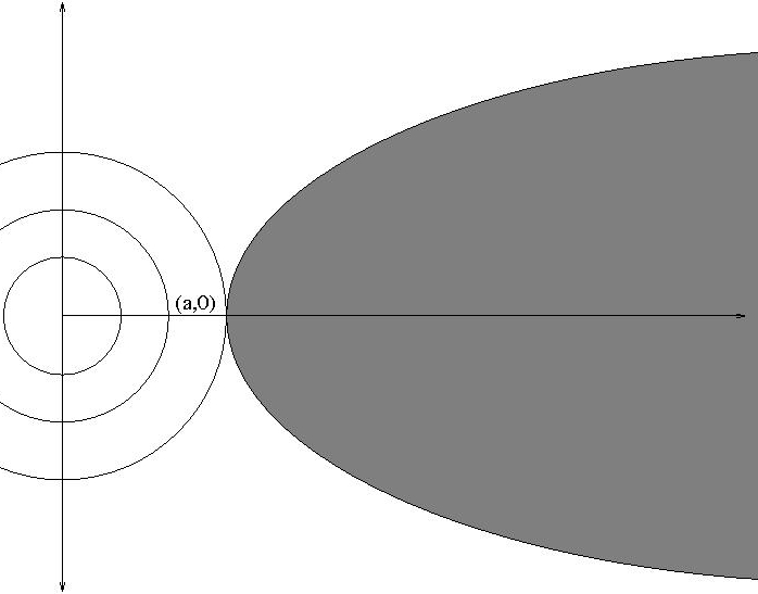
Figure 5: $\mathcal{A}=\{(x^{1},x^{2})|x^{1}\geq(x^{2})^{2}+a\}$.

As $x_{0}$ we choose the point $(a,0)$ which is clearly the dominating point of the set $\mathcal{A}$. Now for any $\theta_{1}>0$ and $\theta_{2}$ it can be shown that

$$c(n,\theta_{1},\theta_{2},a)=\int_{\{\sqrt{n}y_{1}\geq y_{2}^{2}\}}\exp\{-\sqrt{n}(\theta_{1}y_{1}+\theta_{2}y_{2})\}dy_{1}dy_{2}=\frac{\sqrt{\pi}\exp\{\frac{n\theta_{2}^{2}}{4\theta_{1}}\}}{\sqrt{n}\theta_{1}^{\frac{3}{2}}}.$$

Solving $\Lambda^{\prime}(\theta_{1},\theta_{2})=(a,0)$ gives $\theta_{1}^{*}=a$ and $\theta_{2}^{*}=0$. Also

$$\rho_{n,\theta^{*},x_{0}}(t)=\left(\frac{1}{1-\frac{\iota t_{1}}{a\sqrt{n}}}\right)^{\frac{3}{2}}\exp\left\{\frac{-t_{2}^{2}}{4(a-\frac{\iota t_{1}}{\sqrt{n}})}\right\}.$$

Therefore Assumption 3 fails to hold:

$$\lim_{n\rightarrow\infty}\rho_{n,\theta^{*},x_{0}}(t)=\exp\left\{-\frac{t_{2}^{2}}{4a}\right\}.$$

Therefore, in this case the the family of estimator given by (26) may not have asymptotically vanishing relative error. But, nevertheless, it can be shown to have bounded relative error. To see this, note that

$$\int_{v\in\Re^{d}}\rho_{x_{0},\theta^{*}}(A(\theta^{*})v)\phi(v)\,dv=\left(1+\frac{1}{2a}\right)^{-\frac{1}{2}}$$

and

$$\int_{v\in\Re^{d}}\rho_{x_{0},\theta^{*}}(A(\theta^{*})v)^{2}\phi(v)\,dv=\left(1+\frac{1}{a}\right)^{-\frac{1}{2}}.$$

(Here $\Lambda^{\prime\prime}(\theta)={1\,0\choose 0\,1}$ for all $\theta$. So $A(\theta^{*})={1\,0\choose 0\,1}$.) Also $\forall 1\leq i,j,k\leq d$

$$\int_{v\in\Re^{d}}v_{i}v_{j}v_{k}\rho_{x_{0},\theta^{*}}(A(\theta^{*})v)\phi(v)\,dv=0=\int_{v\in\Re^{d}}v_{i}v_{j}v_{k}\rho_{x_{0},\theta^{*}}(A(\theta^{*})v)^{2}\phi(v)\,dv.$$

Therefore as in Proposition 3, it follows that

$$P[\bar{X}_{n}\in\mathcal{A}]\sim\frac{e^{-\frac{na^{2}}{2}}}{2\sqrt{\pi}\sqrt{n}a^{\frac{3}{2}}}\times\left(1+\frac{1}{2a}\right)^{-\frac{1}{2}}.$$

Mimicking the proof of Theorem (2) it can be established that

$$Var_{n}\left[\hat{P}[\bar{X}_{n}\in\mathcal{A}]\right]\rightarrow\frac{1+\frac{1}{2a}}{\sqrt{1+\frac{1}{a}}}-1.$$

Appendix A Proofs

Proof.

(of Proposition 2)
Let $\zeta_{3}(\theta^{*})=\Lambda^{\prime\prime\prime}(\theta^{*})\star A(\theta^{*})$. We have

$$\left|\int_{v\in\Re^{d}}\psi(n^{-\frac{1}{2}}A(\theta^{*})v,\theta^{*},n)\phi(v)dv-1\right| = \left|\int_{v\in\Re^{d}}\{\psi(n^{-\frac{1}{2}}A(\theta^{*})v,\theta^{*},n)-1\}\phi(v)dv\right|$$

$$= \left|\int_{v\in\Re^{d}}\left\{\psi(n^{-\frac{1}{2}}A(\theta^{*})v,\theta^{*},n)-1-\frac{\zeta_{3}(\theta^{*})}{6\sqrt{n}}\odot(\iota v)\right\}\phi(v)dv\right|$$

$$\leq \int_{v\in\Re^{d}}\left|\psi(n^{-\frac{1}{2}}A(\theta^{*})v,\theta^{*},n)-1-\frac{\zeta_{3}(\theta^{*})}{6\sqrt{n}}\odot(\iota v)\right|\phi(v)dv$$

$$= \frac{1}{(2\pi)^{\frac{d}{2}}}(I_{1}+I_{2})\,,$$

where

$$I_{1}=\int_{|n^{-\frac{1}{2}}A(\theta^{*})v|<\delta}\left|\exp\left\{n\times\eta(n^{-\frac{1}{2}}A(\theta^{*})v,\theta^{*})\right\}-1-n\frac{\Lambda^{\prime\prime\prime}(\theta^{*})}{3!}\odot\left(\iota n^{-\frac{1}{2}}A(\theta^{*})v\right)\right|\exp\left\{-\frac{v^{2}}{2}\right\}\,dv,$$

$$I_{2}=\int_{|n^{-\frac{1}{2}}A(\theta^{*})v|\geq\delta}\left|\exp\left\{n\times\eta(n^{-\frac{1}{2}}A(\theta^{*})v,\theta^{*})\right\}-1-n\frac{\Lambda^{\prime\prime\prime}(\theta^{*})}{3!}\odot\left(\iota n^{-\frac{1}{2}}A(\theta^{*})v\right)\right|\exp\left\{-\frac{v^{2}}{2}\right\}\,dv.$$

We now discuss how the $\delta$ above may be selected.

Since $\eta^{\prime\prime\prime}$ is continuous, it follows from the three term Taylor series expansion,

$$\eta(v,\theta)=\eta(0,\theta)+\eta^{\prime}(0,\theta)v+\frac{1}{2}(v)^{T}\eta^{\prime\prime}(0,\theta)v+\frac{1}{6}\eta^{\prime\prime\prime}(\tilde{v},\theta)\odot v$$

(where $\tilde{v}$ is between $v$ and the origin), (10) and (11) that for any given $\epsilon$ we can choose $\delta$ small enough so that

$$|\eta(v,\theta^{*})-\frac{1}{3!}\eta^{\prime\prime\prime}(0,\theta^{*})\odot v|\leq\epsilon(\kappa_{min})^{\frac{3}{2}}|v|^{3}\,\,\,\,\text{for}\,\,|v|<\delta,$$

or equivalently

$$|\eta(v,\theta^{*})-\frac{1}{3!}\Lambda^{\prime\prime\prime}(\theta^{*})\odot(\iota v)|\leq\epsilon(\kappa_{min})^{\frac{3}{2}}|v|^{3}\,\,\,\,\text{for}\,\,|v|<\delta\,.$$ (32)

Since

$$\left|\frac{1}{3!}\Lambda^{\prime\prime\prime}(\theta^{*})\odot(\iota v)\right|<\frac{1}{8}\kappa_{min}|v|^{2}$$ (33)

and

$$|\eta(v,\theta^{*})|<\frac{1}{8}\kappa_{min}|v|^{2}$$ (34)

for all $|v|$ sufficiently small, we choose $\delta$ so that (33) and (34) also hold for $|v|<\delta$.

We apply Lemma (1) with

$$\lambda=n\times\eta\left(n^{-\frac{1}{2}}A(\theta^{*})v,\theta^{*}\right)\,\,\,\text{and}\,\,\,\beta=n\frac{\Lambda^{\prime\prime\prime}(\theta^{*})}{3!}\odot\left(\iota n^{-\frac{1}{2}}A(\theta^{*})v\right).$$

Since $\frac{|\beta|^{2}}{2}=\frac{1}{n}P(v)$, where $P$ is a homogeneous polynomial with coefficients independent of $n$ and for $|n^{-\frac{1}{2}}A(\theta^{*})v|<\delta$ we have from (34), (33) and (32), respectively,

$$|\lambda|=n\left|\eta\left(n^{-\frac{1}{2}}A(\theta^{*})v,\theta^{*}\right)\right|<n\frac{1}{8}\kappa_{min}|n^{-\frac{1}{2}}A(\theta^{*})v|^{2}\leq\frac{1}{8}\kappa_{min}||A(\theta^{*})||^{2}|v|^{2}=\frac{|v|^{2}}{8}\,\,,$$

$$|\beta|=n\left|\frac{1}{3!}\Lambda^{\prime\prime\prime}(\theta^{*})\odot\left(\iota n^{-\frac{1}{2}}A(\theta^{*})v\right)\right|<n\frac{1}{8}\kappa_{min}|n^{-\frac{1}{2}}A(\theta^{*})v|^{2}\leq\frac{1}{8}\kappa_{min}||A(\theta^{*})||^{2}|v|^{2}=\frac{|v|^{2}}{8}$$

and

$$|\lambda-\beta|=n\left|\eta\left(n^{-\frac{1}{2}}A(\theta^{*})v,\theta^{*}\right)-\frac{1}{3!}\Lambda^{\prime\prime\prime}(\theta^{*})\odot\left(\iota n^{-\frac{1}{2}}A(\theta^{*})v\right)\right|<n\epsilon(\kappa_{min})^{\frac{3}{2}}|n^{-\frac{1}{2}}A(\theta^{*})v|^{3}\leq\frac{\epsilon|v|^{3}}{\sqrt{n}}\,.$$

From Lemma (1) it now follows that the integrand in $I_{1}$ is dominated by

$$\exp\left\{\frac{v^{2}}{8}\right\}\times\left(\frac{\epsilon|v|^{3}}{\sqrt{n}}+\frac{1}{n}P(v)\right)\times\exp\left\{-\frac{v^{2}}{2}\right\}=\exp\left\{-\frac{3v^{2}}{8}\right\}\left(\frac{\epsilon|v|^{3}}{\sqrt{n}}+\frac{1}{n}P(v)\right).$$

Since $\epsilon$ is arbitrary we have $I_{1}=o(n^{-\frac{1}{2}})$.

Next we have

$$I_{2} \leq \int_{|n^{-\frac{1}{2}}A(\theta^{*})v|\geq\delta}\left|\exp\left\{-\frac{v^{2}}{2}\right\}\psi(n^{-\frac{1}{2}}A(\theta^{*})v,\theta^{*},n)\right|\,dv$$

$$+ \int_{|n^{-\frac{1}{2}}A(\theta^{*})v|\geq\delta}\left(1+\left|\frac{\zeta_{3}(\theta^{*})\odot v}{6}\right|\right)\exp\left\{-\frac{v^{2}}{2}\right\}\,dv,$$

$$= \int_{|A(\theta^{*})v|\geq\delta\sqrt{n}}\left|\varphi_{\theta^{*}}\left(n^{-\frac{1}{2}}A(\theta^{*})v\right)\right|^{n}\,dv+\int_{|A(\theta^{*})v|\geq\delta\sqrt{n}}\left(1+\left|\frac{\zeta_{3}(\theta^{*})\odot v}{6}\right|\right)\exp\left\{-\frac{v^{2}}{2}\right\}\,dv.$$

Let $q_{\delta}<1$ be such that $|\varphi_{\theta^{*}}(v)|<q_{\delta}$ for $|v|\geq\delta$. Then we have

$$I_{2} \leq q_{\delta}^{n-\gamma}\int_{v\in\Re^{d}}\left|\varphi_{\theta^{*}}\left(n^{-\frac{1}{2}}A(\theta^{*})v\right)\right|^{\gamma}\,dv+\int_{|A(\theta^{*})v|\geq\delta\sqrt{n}}\left(1+\left|\frac{\zeta_{3}(\theta^{*})\odot v}{6}\right|\right)\exp\left\{-\frac{v^{2}}{2}\right\}\,dv,$$

$$= q_{\delta}^{n-\gamma}n^{\frac{d}{2}}\sqrt{|\Lambda^{\prime\prime}(\theta^{*})|}\int_{v\in\Re^{d}}\left|\varphi_{\theta^{*}}(u)\right|^{\gamma}\,du+\int_{|A(\theta^{*})v|\geq\delta\sqrt{n}}\left(1+\left|\frac{\zeta_{3}(\theta^{*})\odot v}{6}\right|\right)\exp\left\{-\frac{v^{2}}{2}\right\}\,dv.$$

It follows that $I_{2}=o(n^{-\alpha})$ for any $\alpha$. ∎

Proof.

(of Theorem 2)
The proof follows along the same line as proof of Theorem 1. We write

$$\int_{v\in\Re^{d}}\frac{\rho_{n,\theta^{*},x_{0}}^{2}(A(\theta^{*})v)\psi^{2}(n^{-\frac{1}{2}}A(\theta^{*})v,\theta^{*},n)\phi^{2}(v)}{g_{n}(v)}\,dv=I_{5}+I_{6}$$

where

$$I_{5} = \int_{|v|<\delta_{2}(n)\sqrt{n}}\frac{\rho_{n,\theta^{*},x_{0}}^{2}(A(\theta^{*})v)\psi^{2}(n^{-\frac{1}{2}}A(\theta^{*})v,\theta^{*},n)\phi^{2}(v)}{g_{n}(v)}\,dv$$

$$= \frac{1}{b_{n}}\int_{|v|<\delta_{2}(n)\sqrt{n}}\rho_{n,\theta^{*},x_{0}}^{2}(A(\theta^{*})v)\psi^{2}(n^{-\frac{1}{2}}A(\theta^{*})v,\theta^{*},n)\phi(v)\,dv.$$

$$I_{6} = \int_{|v|\geq\delta_{2}(n)\sqrt{n}}\frac{\rho_{n,\theta^{*},x_{0}}^{2}(A(\theta^{*})v)\psi^{2}(n^{-\frac{1}{2}}A(\theta^{*})v,\theta^{*},n)\phi^{2}(v)}{g_{n}(v)}\,dv$$

$$= \frac{1}{C_{n}}\int_{|v|\geq\delta_{2}(n)\sqrt{n}}\rho_{n,\theta^{*},x_{0}}^{2}(A(\theta^{*})v)|v|^{\alpha}\psi^{2}(n^{-\frac{1}{2}}A(\theta^{*})v,\theta^{*},n)\phi^{2}(v)\,dv.$$

Now

$$|I_{5}-1| = \left|\frac{1}{b_{n}}\int_{|v|<\delta_{2}(n)\sqrt{n}}\rho_{n,\theta^{*},x_{0}}^{2}(A(\theta^{*})v)\psi^{2}(n^{-\frac{1}{2}}A(\theta^{*})v,\theta^{*},n)\phi(v)\,dv-1\right|$$

$$\leq \frac{1}{b_{n}}\left|\int_{|v|<\delta_{2}(n)\sqrt{n}}\rho_{n,\theta^{*},x_{0}}^{2}(A(\theta^{*})v)\left\{\psi^{2}(n^{-\frac{1}{2}}A(\theta^{*})v,\theta^{*},n)-1\right\}\phi(v)\,dv\right|+o(1)$$

$$\leq \frac{1}{b_{n}}\left|\int_{|v|<\delta_{2}(n)\sqrt{n}}\rho_{n,\theta^{*},x_{0}}^{2}(A(\theta^{*})v)\left\{\psi^{2}(n^{-\frac{1}{2}}A(\theta^{*})v,\theta^{*},n)-1-\frac{\zeta_{3}(\theta^{*})}{3\sqrt{n}}\odot(\iota v)\right\}\phi(v)\,dv\right|+o(1)$$

$$\leq \frac{1}{b_{n}}\int_{|v|<\delta_{2}(n)\sqrt{n}}\left|\rho_{n,\theta^{*},x_{0}}(A(\theta^{*})v)\right|^{2}\left|\psi^{2}(n^{-\frac{1}{2}}A(\theta^{*})v,\theta^{*},n)-1-\frac{\zeta_{3}(\theta^{*})}{3\sqrt{n}}\odot(\iota v)\right|\phi(v)\,dv+o(1)$$

$$\leq \frac{1}{b_{n}}\int_{|v|<\delta_{2}(n)\sqrt{n}}\left|\psi^{2}(n^{-\frac{1}{2}}A(\theta^{*})v,\theta^{*},n)-1-\frac{\zeta_{3}(\theta^{*})}{3\sqrt{n}}\odot(\iota v)\right|\phi(v)\,dv+o(1).$$

Now as in the case of Theorem 1 we conclude that $I_{5}=1+o(n^{-\frac{1}{2}})$. Also, since

$$|I_{6}| \leq \frac{1}{C_{n}}\int_{|A(\theta^{*})v|\geq\delta_{2}(n)\sqrt{n}}|v|^{\alpha}\left|\rho_{n,\theta^{*},x_{0}}(A(\theta^{*})v)\right|^{2}\left|\psi^{2}(n^{-\frac{1}{2}}A(\theta^{*})v,\theta^{*},n)\right|\phi^{2}(v)\,dv$$

$$\leq \frac{1}{(2\pi)^{d}C_{n}}\int_{|A(\theta^{*})v|\geq\delta_{2}(n)\sqrt{n}}|v|^{\alpha}\left|\exp\left\{-v^{2}\right\}\psi^{2}(n^{-\frac{1}{2}}A(\theta^{*})v,\theta^{*},n)\right|\,dv,$$

we conclude that $I_{6}\rightarrow 0$ as $n\rightarrow\infty$ proving the theorem. ∎

References

- [1] Abate, J. and Whitt, W. (1992). The Fourier Series Method for Inverting Transforms of Probability Distribution. Queueing Systems Theory and Applications 10 5–88.
- [2] Abate, J. and Whitt, W. (1992). Numerical Inversion of Probability Generating Functions. Operation Research Letters 12 245–251.
- [3] Asmussen, S. and Glynn, P. (2008). Stochastic Simulation: Algorithms and Analysis. Springer Verlag. New York, NY, USA.
- [4] Butler, R. W. (2007). Saddlepoint Approximation with Applications. Cambridge University Press. Cambridge.
- [5] Blanchet, J. Leder, D. and Glynn, P. (2008). Strongly efficient algorithms for light-tailed random walks: An old folk song sung to a faster new tune… MCQMC 2008.Editor:Pierre L’Ecuyer and Art Owen Springer 227–248.
- [6] Bucklew, J. (2004). An Introduction to Rare Event Simulation. Springer Series in Statistics.
- [7] Carr, P. and Madan, D. (1999). Option Valuation Using Fast Fourier Transform The Journal of Computational Finance. 3, 463–520.
- [8] Carr, P. and Madan, D. (2009). Saddlepoint Methods for Option Pricing. The Journal of Computational Finance. 13 No.1, 49–61.
- [9] Daniels, H. E. (1954). Saddlepoint Approximation in Statistics. Annals of Mathematical Statistics. 25 No.4, 631–650.
- [10] Bucklew, J. A. Ney, P. and Sadowsky, J. S. (1990). Monte Carlo Simulation and Large Deviations Theory for Uniformly Recurrent Markov Chains Journal of Applied Probability, Vol. 27, No. 1 , 44-59.
- [11] Dembo, A. and Zeitouni, O. (1998). Large Deviation Techniques and Applications. 2nd ed. Springer. New York.
- [12] Dey, S. and Juneja, S. (2011). Efficient Estimation of Density and Probability of Large Deviations of Sum of IID Random Variables. To appear in Proceedings of the 2011 Winter Simulation Conference.
- [13] Dieker, A. B. and Mandjes, M. (2005). On Asymptotically Efficient Simulation of Large Deviations Probability. Advances in Applied Probability. 37 No.2, 539–552.
- [14] Feller, W. (1971). An Introduction to Probability Theory and Its Applications Vol.2. John Wiley and Sons.
- [15] Glasserman, P and Juneja, S. (2008). Uniformly Efficient Importance Sampling for the Tail distribution of Sums of Random Variables Maathematics of Operation Research 33 No.1, 36–50.
- [16] Glasserman, P and Li, J. (2005). Importance Sampling for Portfolio Credit Risk Management Science 51 1643–1656.
- [17] Glasserman, P and Wang, Y. (1997). Counterexamples in Importance Sampling for Large Deviation Probabilities The Annals of Applied Probability 7 No. 3, 731–746.
- [18] Iltis, M. (1995). Sharp Asymptotics of Large Deviations in Journal of Theoretical Probability 8 No.3, 501–522.
- [19] Juneja, S. and Shahabuddin, P. (2006). Rare Event Simulation Techniques Handbooks in Operation Research and Management Science 13 Simulation.Elsevier North-Holland, Amsterdam, 291–350.
- [20] Lugnnani, R. and Rice, S. (1980). Saddle Point Approximation for Distribution of the Sum of Independent Random Variables. Advances in Applied Probability 12 No.2, 475–490.
- [21] Jensen, J. L. (1995). Saddlepoint Approximations. Oxford University Press. Oxford.
- [22] Ney, P. (1983). Dominating Points and the Asymptotics of Large Deviations for Random Walk on Annals of Probability 11 No.1, 158–167.
- [23] Parekh, S. and Walrand, J. (1989). A Quick Simulation Method for Excessive Backlogs in Networks of Queue. IEEE Transactions on Automatic Control. 34 No.1, 54–66.
- [24] Rogers, L. C. G. and Zane, O. (1999). Saddlepoint Approximations to Option Pricing. The Annals of Applied Probability. 9 No.2, 493–503.
- [25] Sadowsky, J. S. (1996). On Monte Carlo Estimation of Large Deviation Probabilities The Annals of Applied Probability. 6, 399–422.
- [26] Sadowsky, J. S. and Bucklew, J. A. (1990). On Large Deviation Theory and Asymptotically Efficient Monte Carlo Simulation Estimation IEEE Trans. Inform. Theory 36 No.1, 579–588.
- [27] Scott, L. O. (1997). Pricing Stock Options in a Jump-Diffusion Model with Stochastic Volatility and Interest Rates: Applications of Fourier Inversion Methods Mathematical Finance. 7 No.4, 413–424.