Solar Intranetwork Magnetic Elements: bipolar flux appearance

Abstract

The current study aims to quantify characteristic features of bipolar flux appearance of solar intranetwork (IN) magnetic elements. To attack such a problem, we use the Narrow-band Filter Imager (NFI) magnetograms from the Solar Optical Telescope (SOT) on board Hinode; these data are from quiet and an enhanced network areas. Cluster emergence of mixed polarities and IN ephemeral regions (ERs) are the most conspicuous forms of bipolar flux appearance within the network. Each of the clusters is characterized by a few well-developed ERs that are partially or fully co-aligned in magnetic axis orientation. On average, the sampled IN ERs have total maximum unsigned flux of several $10^{17}$ Mx, separation of $3-4$ arcsec, and a lifetime of $10-15$ minutes. The smallest IN ERs have a maximum unsigned flux of several $10^{16}$ Mx, separations less than 1 arcsec, and lifetimes as short as 5 minutes. Most IN ERs exhibit a rotation of their magnetic axis of more than 10 degrees during flux emergence. Peculiar flux appearance, e.g., bipole shrinkage followed by growth or the reverse, is not unusual. A few examples show repeated shrinkage-growth or growth-shrinkage, like magnetic floats in the dynamic photosphere. The observed bipolar behavior seems to carry rich information on magneto-convection in the sub-photospheric layer.

1 Introduction

The solar surface is often divided in active regions and quiet Sun. The term ‘quiet Sun’ in general refers to regions far from active regions (ARs) where the violent activity, e.g., flares, takes place. However, the ‘quiet Sun’ is never quiet. Many types of small-scale magnetic activity have been revealed, such as microflares (Lin et al., 1987), explosive events in the transition region (Dere et al., 1991), X-ray bright points (Vaiana et al., 1973), X-ray jets (Shibata et al., 1992) and mini-filament eruptions (Wang et al., 2000). They are indicators of an exceedingly dynamic sea of mixed-polarity magnetic fields everywhere on the Sun (Wang et al., 2000), possibly powered by the quiet Sun non-potential magnetic field (Zhao et al., 2009; Yang et al., 2011). Small-scale activity on the Sun, e.g., jets and spicules, can provide a ubiquitous mass supply that is crucial to coronal heating (see De Pontieu et al., 2011).

Network (NT) magnetic elements were known since the 60s (Sheeley, 1967). Intra-network or inner-network (IN) magnetic fields were first described by Livingston and Harvey (1975) and Smithson (1975) as ‘discrete elements’ of mixed polarities ‘interior to the network’. By mid-90s, a few papers (Keller et al., 1994; Lin, 1995; Wang et al., 1995; Lites et al., 1996) largely renewed the interest in the intranetwork field. Great progress has been made (see the recent reviews by de Wijn et al., 2009 and Sánchez Almeida and Martínez González, 2011) since then. With the new Hinode Solar Optical Telescope (SOT) observations, it appears timely to re-examine the key results in this working area and to initiate new efforts to more thoroughly understand this important component of solar magnetism. A few key issues on the physics of the solar intranetwork magnetic field remain to be settled down and require further studies, such as:

1. Intrinsic properties, e.g., the field strength, filling factor, and internal structure. Are the IN elements strong or weak in term of the equipartition magnetic field that has a rough equipartition with the kinetic energy of photospheric plasma flow (Lin, 1995; Solanki et al., 1996; Lin and Rimmele, 1999; Sánchez Almeida and Lites, 2000; Khomenko et al., 2003, 2005; Sánchez Almeida et al., 2003; Socas-Navarro and Lites, 2004; Martínez González et al., 2006; Orozco Suárez et al., 2007a, b; Jin, Wang, and Xie, 2011)? Do they still have internal magnetic structure at the current resolution (see Sánchez Almeida and Lites, 2000)?

2. Flux appearance and disappearance. What is the nature of horizontal magnetic elements (Lites et al., 1996; Harvey et al., 2007; Lites et al., 2008; Ishikawa et al., 2008; Ishikawa and Tsuneta, 2009; Jin et al., 2009a; Ishikawa, Tsuneta, and Jur$\check{c}\acute{a}$k, 2010)? Is there a dominant flux of intranetwork elements in their flux distribution (Wang et al., 1995)? How important are these tiny magnetic elements for the Sun’s magnetic energy supply (Zirin, 1987; Sánchez Almeida, 1998; Trujillo Bueno, Shchukina, and Asensio Ramos, 2004; Thornton and Parnell, 2011; Jin et al., 2011)? How much flux can still be hidden below the spatial scales that can be resolved (Sánchez Almeida and Lites, 2000; Sánchez Almeida, Emonet, and Cattaneo, 2003; Trujillo Bueno, Shchukina, and Asensio Ramos, 2004)? In which ways does the flux disappear from the solar surface? Does flux disappear by magnetic reconnection in the lower solar atmosphere, or by submergence below the photosphere, or by diffusion into unresolved scraps (Livi, Wang, and Martin, 1985; Wang and Shi, 1993; Zhang et al., 1998a; Zhou et al., 2010)?

3. Observed characteristics of magneto-convection. Can we envision how magneto-convection works in the sub-photospheric convective plasma using observations (see Zhang, Yang, and Jin, 2009)? How does the local turbulent dynamo operate in the near-surface layers of the Sun (see Cattaneo, 1999; Sánchez Almeida, Emonet, and Cattaneo, 2003; Vögler et al., 2005; Stein and Nordlund, 2006; Vögler and Schüsler, 2007; Stein et al., 2011)? Is there evidence of the convective collapse in the quiet Sun magnetism (Solanki et al., 1996; Nagata et al., 2008)?

4. Response of the solar atmosphere to the magnetic evolution in the quiet Sun. What is the magnetic nature of network bright points (Dunn and Zirker, 1973; Mehltretter, 1974; Muller and Roudier, 1984; Berger et al., 1995, 2004)? Are we confident about the vision of “magnetic bright points” (see Sánchez Almeida et al., 2004; Sánchez Almeida et al., 2010)? What magnetic quantities and processes determine the heating of the upper atmosphere (Berger and Title, 2001; Ishikawa et al., 2007; Zhao et al., 2009; De Pontieu et al., 2011)?

All quantitative aspects of the above issues are critical in constraining the models of the origin and role of the IN field in solar magnetism and atmospheric heating.

In earlier papers, we have described the life-story and lifetime of IN magnetic elements (Zhou et al., 2010) and studied the intrinsic properties of intranetwork and network elements including the field strength, filling factor, inclination, and other aspects (Jin, Wang, and Xie, 2011). The IN elements are found to be intrinsically weak in term of the equipartition field strength. This paper is focused on the IN flux appearance in the form of bipolar emergence, shrinkage and submergence. Our main motivation is to explore the interaction of magnetic and convective fields in the photosphere and immediate sub-photosphere.

Based on the SOT/Spectro-polarimeter (SP) and SOT/FGIV observations onboard Hinode, which have improved the spatial resolution and polarization sensitivity, flux appearance at IN scale has been amply studied. Centeno et al. (2007) reported an event of bipolar emergence within a quiet granule. Extended examples of bipolar emergence have been studied by Martínez González and Bellot Rubio (2009). These authors find that a significant fraction of the magnetic flux in IN regions appears in the form of $\Omega$-shaped loops with an emergence rate of 1.1$\times 10^{12}$ Mx s^-1 arcsec^-2, which corresponds to 8.38$\times 10^{26}$ Mx per day for the whole Sun. Unipolar flux emergence has been studied by Lamb et al.(2010). They find it likely that the coalescence of weak flux leads to the appearance of unipolar flux elements. Orozco Suárez et al. (2008) describe a particular example of vertical field emergence; the emergence of horizontal magnetic elements has been reported by many authors (see Ishikawa and Tsuneta, 2009). Ishikawa and Tsuneta (2009) distinguished the buoyancy-driven emergence (type 1) and the convection-driven emergence (type 2). The later is related to the horizontal magnetic elements. Zhang, Yang and Jin (2009) examined the interaction of flux emergence and granulation. Jin, Wang and Zhao (2009b) obtained the vector magnetic field distribution in solar granules. These observations provide a rich set of information on the magneto-convection in the layer immediately beneath the photosphere. With the unprecedented spatial resolution and polarization sensitivity from Hinode and new ground-based observations, we seem to be at a critical moment to diagnose or even to image the subsurface magneto-convection. It is also worth to mention that remarkable progress in numerical simulations of magneto-convection has been made (see Cheung et al., 2008). The simulations have shed new light in understanding the recent observations.

In this study we use SOT/Narrow-band Filter Imager (NFI) magnetograms to particularly explore magnetic bipolar appearance in IN regions. Emergence in clusters of mixed polarity and IN ephemeral regions are exemplified, and a peculiar pattern of bipolar shrinkage-growth, and/or growth-shrinkage, like a magnetic float in convective plasma, is described for the first time.

The next section is devoted to the description of observations and calibration methods. Section 3 is devoted to the detailed description of magnetic bipolar appearance in the form of clusters, IN ephemeral regions and float-like bipoles. Conclusions and discussion will be presented in the last section.

2 Hinode SOT/NFI Observations

2.1 Why are SOT/NFI observations needed?

This series of studies is mostly based on Hinode SOT/NFI data. The basic reason to choose SOT/NFI data comes from the following considerations. SOT/NFI data have adequate temporal resolution, e.g., 1-2 minutes, in addition to high spatial resolution of 0.3 arcsec. We can follow many magnetic elements in a large field of view. The selection of IN bipoles is much less ambiguous when the temporal behavior can be taken into account. Moreover, the evolution of the magnetic bipoles can be followed for a reasonable time interval in order to understand their appearance and disappearance. Using the simultaneous filtergrams obtained by Hinode/SOT, we can diagnose the chromospheric response to the magnetic evolution, a study that we defer for a later time.

2.2 Selected quiet regions

Two regions are selected for this study. They are listed in Table 1. The pixel size for the observations of both regions is 0.16 arcsec, and the spatial resolution is 0.32 arcsec. The analysis is made for the time-sequence of the quiet-network region (QNT) on 24 June 2007 (see Figure 1) and the enhanced-network region (ENT) on 11 December 2006 (see Figure 2). The ENT is to the east of NOAA active region (AR) 10930 and covers partially the AR plage. To the west in the center of Figure 2, the outer boundary of a sunspot penumbra is marked by dashed curved line. For the quiet network region, the temporal resolution is 1 minute; while for the enhanced network region it is 2 minutes. In Table 1, we list two other quiet-network regions in lines 2 and 3 for a future study on the flux distribution (Zhou, Wang, and Jin, 2011). All the quiet regions are located close to disk center.

Table 1.: The studied ENT region and QNT regions. tbl-0

dates	Obs. (UT)	Wavelenth (Å)	Pos.	FOV (pix2)	Charac.
Dec. 11 2006	19:08-23:58	FeI 6302	S10E01	638$\times$788	ENT
Dec. 19 2006	23:56	FeI 6302	S00E10	626$\times$782	QNT
Dec. 20 2006	06:36	FeI 6302	S00E02	751$\times$783	QNT
June 24 2007	17:12-18:09	NaI 5896	S00W10	932$\times$894	QNT

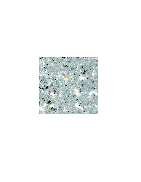
Figure 1.: The SOT/NFI line-of-sight magnetogram at 17:36:50 UT, 24 June 2007, is scaled in the range of $\pm$ 50 G. A bar in the lower-right corner indicates a 10 arcsec length. The framed boxes correspond to the windows discussed in text; from top to bottom: IN ERs (framed by solid lines), peculiar flux appearance (by dashed-dotted lines), and cluster emergence of mixed polarities (by dashed lines). In the lower part of the magnetogram, a complete network cell is marked by a circle. A few tiny IN ERs are marked by small yellow circles, while cancelling magnetic features (CMFs) are identified as red squares. Here and in the following figures, north is to the top and east, to the left.fig1

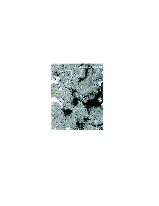
Figure 2.: The SOT/NFI line-of-sight magnetogram at 20:50:43 UT, 11 December 2006, is drawn in the same style as for Figure 1. A bar in the lower-right corner indicates a 10 arcsec length. The box framed by dashed lines shows an area of cluster flux emergence, while an adjacent box drawn with dot-dashed lines shows a flux convergence center. Red boxes and yellow circles have the same meaning as in Figure 1. fig2

Extremely rich information about IN bipolar appearance, evolution and disappearance is exhibited by Hinode SOT/NFI observations, though it is not easy to describe. In this study we try to explore and show the most conspicuous behavior of bipoles during their appearance, not revealed by earlier ground-based observations with lower spatial resolutions. A few sub-fields in each of the magnetograms in the chosen time intervals, selected rather randomly, are used for our exploratory work. We leave for further studies a more complete statistic description of the properties of the flux evolution of IN magnetic elements.

2.3 Calibration of flux measurements

Following the procedure suggested by Chae et al. (2007), we calibrate the magnetic flux measurements by comparing the SOT/NFI observations adopted in this study, with quasi-simultaneous SOT/SP observations. For each of the four quiet regions, we selected a subfield for which NFI and SP observations were taken quasi-simultaneously. For each subfield to match temporarily the two types of observations, we created a combined NFI magnetogram with stripes taken from the magnetograms at different times which are as close as possible to the scanning interval of Stokes V profiles in SP observations. In this way, the observed magnetic structures are present almost at the same time in both NFI and SP observations (see the top panels of Figure 3). In the present paper, we use the same calibration and procedure as in Zhou et al. (2010).

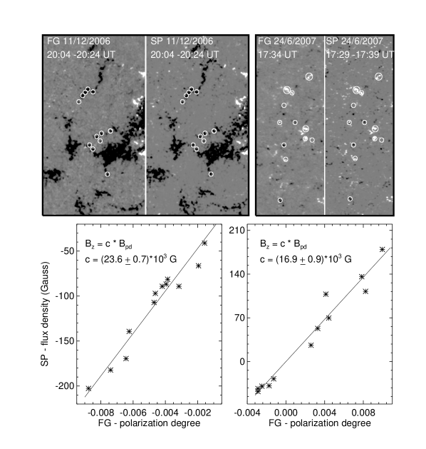
Figure 3.: Top panels: quasi-simultaneous SOT/NFI and SP line-of-sight magnetograms for selected windows. The SP magnetograms are reconstructed from an inversion of Stokes V profiles using an ME atmospheric model. The SP magnetogram has been scaled to the dynamic range of $\pm 300$ G; while for that of SOT/NFI, the dynamic range of V/I is set to $0.014$. From each pair of magnetograms, a few well-defined NT elements are selected and encircled. Bottom panels: correlation of SOT/NFI V/I and the inverted flux density from SP V/I profiles. The slope found for each set of observations is used to calibrate the NFI magnetograms.fig3

As demonstrated by Chae et al. (2007), for flux densities $<$ 1 kG a linear relationship exists between the observed flux density in NFI observations and the ‘true’ flux density, obtained from the inversion of SP data. Therefore, it is meaningful to select a few well-defined NT magnetic elements and obtain a calibration constant by forcing the measured flux of these elements to be the same in both types of observations. The relationships for both ENT and QNT are shown in the bottom panels of Figure 3. For the observations of ENT regions taken in the FeI 6302 Å line, the calibration coefficient falls in the range of 23600$\pm$700 G, while for the observations of the QNT region in the NaI 5896 Å line, the calibration coefficient is 16900$\pm$900 G. The calibration coefficient is higher than for other filter-based magnetographs operated on the ground (see Wang et al., 1996), but consistent in order of magnitude. The magnetograms taken in NaI 5896 Å appear to be more sensitive than those taken in FeI 6302 Å.

2.4 Apparent oscillation of the IN flux density

There are very clear signals of oscillations in the apparent flux density observed in the IN regions, with a magnitude of $\pm$1 G around the mean background flux density. In Figure 4, the average net flux density of a very quiet IN area within a typical network is shown.

Figure 4.: Mean net flux density within a network marked by a circle in Figure 1. The solid line is the measured mean net flux density, with the fitted curve indicating the general trend of the background flux density changes with time. The dotted line represents the standard deviation of the mean net flux density. To include the plots in the same figure, 34.0 G were subtracted from the standard deviation curve.fig4

Within approximately 63 minutes, 15 cycles of flux density variation appear, indicating an oscillation with a period of 4.2 minutes. At present, it is not clear whether this oscillation of the net flux density is a real magnetic oscillation, i.e., of magnetic origin, or the manifestation of Doppler remnants in the magnetic flux measurements.

Although the magnitude of the oscillation, as we measured for many network cells, is no more than $\pm$ 1-2 G, the average net flux density changes with time; see the fitted curve for the net flux density in Figure 4. This would mean that there is a changing background polarization in the flux measurements, which affects those for weak magnetic features. Moreover, the oscillation would cause mis-identification of tiny weak magnetic elements. Therefore, in this set of studies, whenever necessary, we perform a temporal average to reduce the oscillation effects.

3 Magnetic bipole appearance

3.1 In clusters of mixed polarities

The analysis of Hinode data has fully confirmed earlier observations of a flux emergence center which appears somewhere within the network (Wang et al., 1995). In such an emergence center, IN flux appears in the form of a cluster of mixed polarities.

An example of a flux emergence center in the QNT region is shown in Figure 5 (see also Figure 1). In the upper-left of the figure there is an emergence center, where a cluster of mixed polarities started to show up from 17:31 UT. The cluster reached its maximum development at 17:46 UT and faded after 17:50 UT, suggesting a lifetime of about 30 minutes. We have clearly observed that in this cluster of mixed polarities, there were, at least, 4 ephemeral regions (ERs) which are marked in the figure by green ovals. Their flux density, size, and location fall into the typical categories of IN magnetic elements. In this paper, we call them as intranetwork ephemeral regions (IN ERs). Two of the IN ERs showed the same magnetic axis orientation, suggesting one or two co-aligned flux bundles emerging in the convective plasma. The maximum unsigned flux of each ER in the cluster is (5.9$\pm$2.0)$\times 10^{17}$ Mx in average, and the separation of the two polarities, 3.3$\pm$2.1 arcsec. The positive flux of these ERs is dominant in this cluster.

Since 17:35 UT, another cluster appeared in the lower-right part of the field of view (FOV). Three larger ERs, each with total unsigned flux larger than $10^{18}$ Mx, are identified and marked by green ovals. They were generally co-aligned, indicating the emergence of a bundle of magnetic flux from below. Flux cancellation within the cluster seem to suggest a serpentine structure of the flux bundle near the surface (see Cheung et al., 2008). However, it is noticed that in SOT/NFI observations the small-scale emerged flux is always in the form of point-like flux patches instead of sheets. From ground-based observations of the highest spatial resolution, the smallest magnetic field structures appear to arise from isolated points in the intergranular lanes, instead of arising as continuous flux sheets confined to the lanes (Goode et al., 2010).

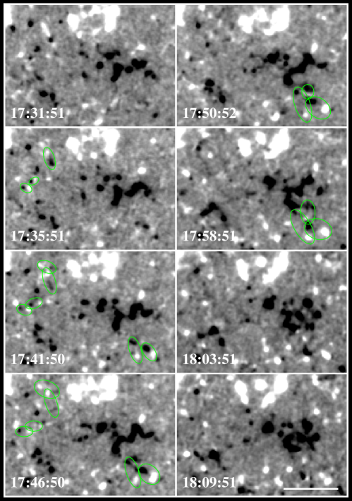
Figure 5.: Time-sequence of magnetic flux evolution in the flux emergence center framed with dashed lines in Figure 1. A bar in the lower-right corner indicates a length of 10 arcsec. An emergence center in the upper-left corner appeared since 17:31 UT and faded after 17:50 UT. In the cluster of mixed-polarity elements, 4 IN ERs are marked by green ovals. Another cluster emergence started later at 17:35 UT in the lower-right corner of the FOV, in which 3 larger ERs were identified.fig5

A flux emergence center within a network in the ENT region is shown in Figure 6 (see also Figure 2). A cluster of mixed polarities first appeared at 20:10 UT in the lower-left of the FOV and flux emergence extended later to the middle and upper parts. In this cluster 4 IN ERs are clearly identified. Its maximum development took place at approximately 20:20 UT. In the decay phase of the cluster, one ER grew up and became a relatively large ER with total unsigned flux close to $10^{18}$ Mx by 20:32 UT. Moreover, another ER emerged in the same location and showed the same magnetic orientation, even though the cluster had already disappeared. The lifetime of this cluster was about 30 minutes. As for the cluster described in Figure 5, most of the identified IN ERs in this cluster have roughly the same magnetic orientation. Again, another cluster started to emerge at 21:04 UT in the upper-right corner of the FOV, in which at least one or two IN ERs show up clearly.

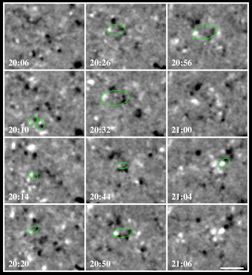
Figure 6.: Time-sequence of the magnetic flux evolution in the flux emergence center framed in Figure 2 with dashed lines. A bar in the lower-right corner indicates a 10 arcsec length. An emergence center in the lower left corner appeared at 20:10 UT and faded after 20:26 UT. In this cluster of mixed polarities, 4 IN ERs are marked by green ovals. Later at 21:04 UT another cluster started to emerge in the upper-right corner of the FOV. One ER was clearly seen and marked by a green oval.fig6

In earlier ground-based observations (Wang et al., 1995), we occasionally found small bipoles, i.e., ERs, could be identified in the cluster of mixed polarities. With Hinode SOT/NFI data, the largely improved spatial and adequate temporal resolutions enable us to reveal that in each of the clusters there are always a few well-defined ERs. Most of the IN ERs in a cluster have a total unsigned flux less than $10^{18}$ Mx, while the total unsigned flux of each cluster is several times $10^{18}$ Mx. The cluster behavior, e.g., the rather ordered alignment of mixed polarities and a few clearly identified ERs, seem to be consistent with the predicted picture of the serpentine field lines that emerge into the photosphere in magneto-convection simulations (see Cheung et al., 2008 and the references therein). However, the total flux for each well-observed cluster is much less than the one in the simulation, e.g., from several times $10^{19}$ Mx to $10^{20}$ Mx. The observed clusters seem to exhibit interlaced and braided features as in an emerging bundle of magnetic flux. However, even with one minute temporal resolution and 0.3 arcsec spatial resolution, we are unable to identify the magnetic connectivity of all the mixed polarity elements in an observed cluster.

It is interesting to see that sometimes within the same network, a flux convergence center is just located in adjacent to a flux emergence center (see the one framed by a dash-dotted line in Figure 2). The flux convergence is shown in Figure 7. It is not difficult to see the general convergence of magnetic elements toward to the center of the FOV. For the two negative elements which converged toward the center of the FOV and merged into an element, the average convergence speed was about 4.0 km$s^{-1}$ from 20:22 to 20:52 UT. Flux convergence is usually achieved by converging motions and flux cancellation of IN elements of opposite polarity.

In cases of flux coalescence of the same polarity flux patches, we always observe their cancellation with opposite polarities between them. The isolated merging of same polarity patches without flux cancellation with surrounding opposite polarities has never been found. This fact was previously recognized in our early ground-based observations (e.g., Wang et al., 1995).

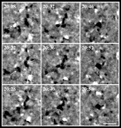
Figure 7.: Time-sequence of magnetic evolution in the flux convergence center framed with a dot-dashed line in Figure 2. A bar at the lower-right corner indicates a 10 arcsec length. Arrows in the figure mark 3 elements which moved rapidly to the center of the FOV with a speed above 4 km$s^{-1}$.fig7

3.2 Intranetwork ephemeral regions

For the sampled QNT and ENT regions, lots of tiny ERs within the cells of the magnetic network are identified. They typically have the size and flux of IN magnetic elements. Hereby we refer to them as intranetwork ephemeral regions (IN ERs). A statistical analysis of IN ERs is undertaken.

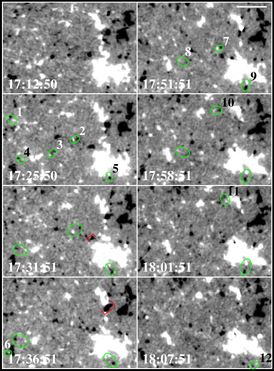
Figure 8.: Illustrations of IN ERs for the area of a network cell framed in Figure 1 by the solid lines. A bar in the upper-right corner indicates a 10 arcsec length. Twelve IN ERs emerged in this area, each of which is marked by a green oval in the figure, from 17:13 to 18:08 UT.fig8

In an area of 45$\times$31 arcsec², approximately the size of a supergranular cell, and in an interval of 55 minutes (Figure 1) we identified 12 likely ERs. They are numbered in Figure 8 according to the time of first appearance. Most of them are not difficult to follow in the successive frames in the figure. Their magnetic axis distribution is random. The average maximum unsigned flux, separation, and lifetime of the 12 IN ERs are (7.8$\pm$4.1)$\times 10^{17}$ Mx, 3.3$\pm$1.4 arcsec, and 14$\pm$8 minutes, respectively. The ERs emerged close to strong NT elements tend to have more magnetic flux. In Figure 8, ERs 5 and 9 emerged in the strong network boundary and close to strong positive NT elements. Their total unsigned fluxes were 1.48 $\times 10^{18}$ Mx and 1.41$\times 10^{18}$ Mx, respectively, which are still two orders of magnitude smaller than those first reported by Harvey and Martin (1973), and one order of magnitude smaller than the average flux found by Heganaar (2001). Careful statistical work needs to be done to distinguish (if possible) between IN ERs and other ‘normal’ ERs as described in the earlier literature.

In Figure 8 we mark two cancelling magnetic features with red square brackets at 17:31 and 17:36 UT, respectively. Two adjacent flux patches of opposite polarity are not necessarily ERs, but often pseudo ERs though they are paired in the close vicinity (Martin et al., 1985). For example, at 17:36 UT, a negative NT element (marked with a red square bracket) and the adjacent positive NT element of about the same size looked like an ER. However, looking at their evolution, we find that they moved toward one another, the magnetic gradient between the opposite polarities increased, and their flux disappeared mutually. This is a typical cancelling magnetic feature (CMF) consisting of two NT elements of opposite polarity (Livi, Wang, and Martin, 1985; Wang et al., 1988). An IN element of negative polarity, which was marked at 17:31 UT in the figure, intruded into the strong positive network elements and cancelled with them. By 18:01 UT it was encircled entirely by NT positive flux, and disappeared completely after 18:07 UT. The scenario is very typical of flux cancellation between IN and NT elements.

  

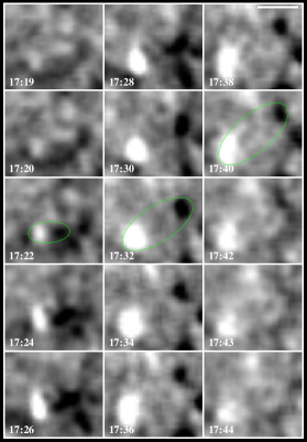
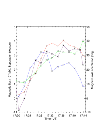
                 (a)                                (b)

Figure 9.: Panels (a): illustration of ER2 from the earliest appearance to the disappearance of its negative polarity. The bar in the upper-right corner indicates a length of 2 arcsec. Panel (b): curves indicating the evolution of the magnetic flux, separation, and magnetic orientation of ER2. The positive flux is drawn in red and marked by Plus symbol, negative flux, in blue and by Cross symbol. The separation of the two polarities is shown in green and by Square symbol, and the magnetic orientation from the positive to the negative polarity in dark purple and by Asterisk symbol. Note, the flux, separation, and orientation have different scales though they share the same ordinate. The magnetic flux is expressed in units of $10^{17}$ Mx, the separation in units of 1 arcsec, and the orientation in units of 10 degrees being the angle positive for an anti-clockwise rotation starting from the solar equator.fig9

The appearance of ER2 is shown in Panels (a) of Figure 9, and the flux evolution, separation, and magnetic orientation of its polarities are shown in Panel (b). Although being a simple ER, it had a complicated interaction with the surrounding magnetic flux. Both poles of ER2 did not fully grow while cancelling with nearby opposite polarities. The negative pole seemed to be clustered with nearby flux of the same polarity and embodied in the unresolved flux of opposite polarity with very low flux density. It never grew as strong as its positive counterpart. The most rapid separation, growth and rotation took place from 17:24 to 17:30 UT in the early phase of flux emergence. It is remarkable that this IN ER rotated anti-clockwise for more than 30⁰ with a rotating rate of approximately 0.08⁰ s${-1}$ (see Panel (b) of Figure 9). The fast magnetic axis rotation is co-temporal with the flux growth. The evolution of these characteristics of ER2 are common to other IN ERs in this study.

Moreover, even with a 1 minute cadence, it is not straightforward to identify the same ER in two successive Hinode/NFI frames. The identification of ERs is affected by problems due to a low temporal resolution in three cases: 1) an ER with a shorter lifetime, 2) an ER subject to complicated interactions with the surrounding magnetic elements, and 3) an ER displaying convective motions. Often, the identification is difficult and uncertain, as in the case of ER5 and ER9. We are not sure if they are a single ER or two ERs, or even some peculiar flux appearance. We will discuss them in the next section.

According to the traditional definition for an ER, the two flux patches with opposite polarity emerge simultaneously or one following the other, and grow and separate co-temporally (see Harvey and Martin 1973). Hinode data extend the identification of ERs to those with much lower flux. It has long been believed that ERs represent small-scale bipole loop emergence (see Parker 1984). The ERs shown here are the same as the emerging small-scale magnetic loops, described observationally by Centeno et al. (2007) and Martinez Gonzalez and Bellot Rubio (2009). In Figures 1 and 2, we marked a few tiny IN ERs by green circles. They all meet the above definition for an ER and their emergence can be traced at least in three successive frames. The ERs on the quiet Sun may have a total unsigned flux less than 10¹⁷ Mx and separation less than 1 arcsec.

Figure 10.: Top panels: a tiny ER in shown by contours of the flux density. Its total unsigned flux is about $1.0\times 10^{17}$ Mx and the separation less than 1 arcsec. Middle panels: a tiny CMF is shown by contours of the flux density. Bottom panels: a tiny ER shown by contours of the flux density. The axes are in arcsec. The contour levels are $\pm$10, 20, 30, 50 G, respectively. fig10

In the top panels of Figure 10, the emergence of a tiny ER (marked as the uppermost green circle in Figure 1) is shown by contours of the magnetic flux density. It fitted exactly the definition of an ER and showed imbalance magnetic flux between opposite polarities in its later development. The flux imbalance of this ER resulted from the merging of its positive pole with a nearby positive flux. Moreover, its magnetic axis rotated anti-clockwise for more than 20 degrees in 5 minutes. In the bottom panels of Figure 10, another tiny ER (marked by a green circle in the central part of Figure 2) is shown in the same way. Its positive pole is in the center of the FOV and the negative one to its north. As usual, this ER exhibited flux imbalance between opposite polarities. The imbalance is caused by the cancellation of the ER’s positive pole with the negative flux to its south. The positive pole grows and simultaneously cancels with a nearby negative flux patch. As the result of flux cancellation, the negative flux patch in the south showed a rapid decrease both in area and flux density and the ER positive pole never grew as strong as the negative one. It is important to notice that even at the smallest spatial scale, IN ERs follow the typical scenario in emergence as larger ERs (Schrijver and Zwaan, 2001; Thomas and Weiss, 2008). Often, an apparent bipole with approximately the same flux and size, e.g, the apparent bipole at 20:50 UT in the lower-left of the FOV in the bottom panel, is not an ER. The automatic selection of ERs from magnetograms with poor temporal resolution should be considered with great cautions (see Hagenaar, 2001).

A few tiny CMFs are marked in Figures 1 and 2 by small red squares. One of them is shown in the middle panels of Figure 10 (marked by a small red square in the middle-right of Figure 1). Its negative pole is in the middle of the FOV. The positive pole grew from 17:35 to 17:40 UT by coalescence with a positive polarity to its north-west. The cancellation, as usual, started first at the place where there were high field gradients. As the result of flux cancellation, the negative flux fragmented into two pieces, one of them was very small. The positive flux tended to move toward the cancellation site. From the curvature of the periphery of the positive flux, we know where flux loss had taken place. The negative flux disappeared completely from 17:40 to 17:43 UT. The scenario is very much typical of any CMF though happening between tiny flux patches of opposite polarity.

3.3 Peculiar flux appearance and magnetic float

Observations of flux submergence have been reported for ARs using early ground-based observations (Wallenhorst and Topka, 1982; Rabin et al., 1984; Zirin, 1985; Harvey et al., 1999; Kalman, 2001). These observations sometimes were considered to be questionable as the spatial and temporal resolutions were not high enough and in most of the cases no vector field observations were available in the analysis. Yang et al.(2009) reported an example of flux submergence of an ER in a coronal hole observed with Hinode high spatial resolution. It is worthwhile emphasizing that the term of flux “submergence” implies the physical scenario of an $\Omega$ loop that once broke out into the photosphere from below and now retracted into the sub-photosphere again. Without 3-D magnetic observations, including data from the sub-photospheric layers, it is really hard to believe that the observed submergence is real. Therefore, the term “submergence” is used in this paper to describe that the opposite polarities of an ER reverse their growth and separation.

Figure 11.: Time evolution of an ER, ER 3 in Figure 8, shown by contour maps of magnetic flux density. The axes are in arcsec, and the contour levels are $\pm$10, 20, 30, 50 G, respectively.fig11

Among all the ERs described above, only ER3 in Figure 8 exhibited the unusual scenario of flux emergence followed by an apparent submergence. In Figure 11, we show the whole evolution of ER3 with contour maps at one minute cadence. In this way, the quantitative evolution can be viewed more clearly. The ER seemed to emerge partially in pre-existing flux. From the earlier appearance of the ER at 17:23 UT to the disappearance of its negative polarity at 17:46 UT, the evolution can be divided in steps: (1) clearing up the bipole emergence from 17:24 to 17:28 UT, during which a portion of the negative pole separated and cancelled with the pre-existing positive pole while moving outward; (2) evolving to its maximum development at 17:34 UT when its negative pole became strongest in flux density and its positive pole showed up the secondary flux center (with a contour value of 20 G); (3) setting up for submergence in the interval of 17:34 to 17:41 UT, during which its positive pole had its secondary flux patch cancelled with the ER negative pole and its positive flux coalesced; (4) shrinkage of the bipole from 17:41 to 17:47 UT. The first and third steps are complicated and involve interior cancellation between pieces of flux of two opposite polarities and external cancellation with surrounding opposite polarities. After these two steps, the ER seemed to strip the surrounding flux and appeared as a more simple bipole. It is interesting to notice that the magnetic axis of the overall bipole rotated clockwise in the first two steps for about 30 degrees. Then in step 3, it rotated back anti-clockwise, and finally in step 4, the axis rotated clockwise again close to east-west direction. From this and other examples, we have learned that the magnetic axis of an ER always rotates rapidly during rapid flux growth and shrinkage.

To our knowledge, this is the first evidence of a bipole emergence followed by apparent submergence, i.e., an ER cancelling itself. We believe that there is a bipole emergence and submergence because we track the two opposite polarities continuously at high enough cadence and spatial resolution.

Although it is not often to see an ER cancelling itself, quite a few examples show the opposite process, a cancelling magnetic feature that finally reverses its evolution and appears as an ER. In Figure 12, we show a pair of opposite polarities approaching and cancelling from 17:42 - 17:53 UT. However, after the opposite polarities appeared to come into contact, they reverse their evolution. A pair of polarities with almost the same flux started to grow and separate like a usual ER. This can be seen until the negative flux disappeared. For comparison, a normal ER is surrounded with a green oval in the first three magnetograms. The ER grew and separated during the whole time-sequence, a very clear example of “direct emergence” (see Toriumi and Yokoyama, 2010).

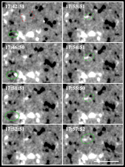
Figure 12.: A cancelling magnetic feature is marked by open square brackets at 17:42 UT. After approach and cancellation of opposite polarities for 10 minutes, the bipole, marked by a dashed green oval, appears to separate from 17:53 UT as a usual ER. To compare, an ER at the NT boundary is shown by a solid green oval. A bar at the lowest right corner indicates a length of 10 arcesec.fig12

Sometimes, a bipole is seen to shrink first, then, to grow for some time, and to shrink again. In the process of shrinkage-growth-shrinkage its magnetic axis rotates greatly. An example of this type of flux evolution is shown in Figure 13. The first shrinkage took place from 17:30 to 17:42 UT. The shrinkage was followed by growth from 17:42 to 17:50 UT. The bipole shrank again after 17:50 UT. The negative polarity of the bipole disappeared after 17:54 UT. The flux decrease and increase in the negative pole was companied by the co-temporal decrease and increase in the positive polarity. During this evolution, the magnetic axis rotated clockwise from about 40 degrees to -80 degrees. The negative pole rotated around the stronger positive pole for more than 100 degrees with a rotating rate of 0.1 degrees/s (for rapid sunspot rotation see Zhang, Li, and Song, 2007 and Yan et al., 2009). The bipole shown here looks like a magnetic float in the convective photosphere, i.e., the $\Omega$-loop is observed to sink, rise, and sink again while rotating.

Figure 13.: A bipole showing shrinkage-growth-shrinkage during a time interval of 20 minutes. fig13

The evolution of ER5 and ER9 in Figure 8 is complex (see Section 3.2). Observationally, analyzing a short time interval with an intermittent image sampling, we would have no doubts that their evolutions were consistent with two ERs. However, if we viewed the evolution in a longer interval and with higher cadence, we would find that the evolution was very complicated (see Figure 14). We could not be sure if we did observe two ERs or just one ER with a peculiar evolution.

First, we saw two opposite polarity elements which moved closer from 17:20 to 17:25 UT while their flux slightly decrease, e.g., characteristic of a “cancelling magnetic feature”. Secondly, from 17:25 to 17:34 UT, we basically saw the separation and some flux increase of these two opposite polarities, although interacting with other smaller magnetic elements. Even with one minute cadence, we could not ascertain if the negative polarity that we saw at 17:34 UT was the same as that at 17:25 UT. Thirdly, we could only tentatively conclude that only an ER (marked as ER5 in Figure 8) was observed. Notice that from 17:27 to 17:31 UT additional negative flux patches, whose magnetic connectivity was hard to tell, appeared. Fourthly, from 17:34 UT, we seem to see another cancelling magnetic feature, i.e., the approach and shrinkage of opposite polarities until 17:48 UT. Finally, another ER (marked as ER9 in Figure 8) was seen from 17:48 to 18:09 UT. The fast separation of opposite polarities seemed to really represent a buoyant flux emergence with an increase of the magnetic field strength.

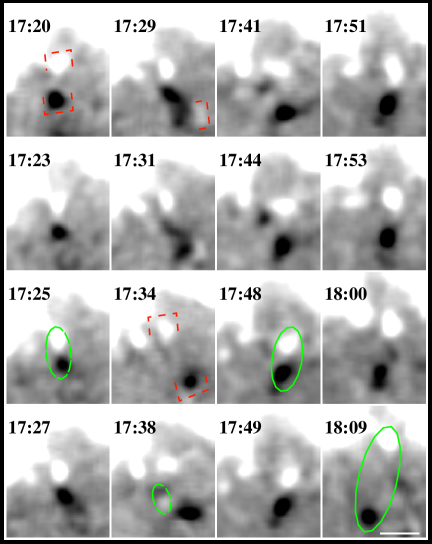
Figure 14.: A bipole showing double shrinkage-growth during an hour. The bar in the lowest-right corner indicates a length of 2 arcsec.fig14

It is interesting to notice that the total flux of this bipole changed in the range of (8 - 15)$\times 10^{17}$ Mx, i.e., within a factor of two. We have not observed a rapid flux emergence like the one in other ERs or fast CMF-like flux disappearance. We seem to witness a floating bipole suspended in the dynamic photosphere, moving up and down, while changing its orientation slightly. The other examples shown in Figures 11 to 13 also seem to show a magnetic float, at least, during some interval in their lifetime.

The magnetic float behavior is quite commonly seen in SOT/NFI magnetograms with high spacial resolution and adequate cadence. From another view point, we may be observing the complexity of flux emergence, “two-step emergence” or multiple-step emergence, or even “failed emergence”, as suggested in the numerical simulation by Toriumi and Yokoyama (2010). The magnetic fields in the complicated flux emergence is not so strong but within the typical range of intranetwork fields (see Jin, Wang, and Xie, 2011).

The behavior of magnetic floats implies that these IN bipoles are close to an equilibrium between magnetic and convective drag forces. It is assumed that the importance of the drag force increases with decreasing tube radius and that tubes can be dragged even if they have strong magnetic fields of the order of thousands of Gauss (see Sánchez Almeida, 2001 and references herein). However, as Jin, Wang, and Xie (2011) demonstrated, the IN fields are dominantly weak in terms of the equipartition field with the convection in the photosphere. The destiny of a floating bipole is either to emerge due to a magnetic buoyancy instability when the magnetic field is enhanced in the flux loop, or to submerge forced by local convection together with magnetic tension, or breaking up into fragments by interacting with other magnetic elements.

4 Conclusions and Discussion

With the unprecedented spatial resolution of SOT/NFI magnetograms, we have confirmed the existence of flux emergence centers which appear somewhere within the network as earlier found (Wang et al., 1995). IN flux appears in such an emergence center in the form of a cluster of mixed polarities. It has been further clarified that in each of the clusters there are always a few well-developed ephemeral regions, whose magnetic orientation appears to be in general the same.

The sampled IN ephemeral regions have fluxes from less than 1$\times 10^{17}$ Mx to 15 $\times 10^{17}$ Mx, separations of the two polarities from 3 arcsec to 4 arcsec, and lifetimes of 15-20 minutes. The smallest IN ERs have a maximum separation between opposite polarities of less than 1 arcsec, and a total unsigned flux of a few times of $10^{16}$ Mx.

We have shown that many IN bipoles behave like a magnetic float in the convective photosphere. They are often found to first shrink and then grow, or vice versa during a time interval of several tens of minutes. The scenario of shrinkage-growth and/or growth-shrinkage implies that these IN bipoles are in a quasi-equilibrium in the photosphere. They are likely to have an equipartition field strength with plasma kinematics, and are buffeted again and again by plasma convection.

The force keeping a magnetic bipole in an equilibrium can be simplified as

$$F=\frac{B_{i}^{2}}{2\mu\Lambda_{e}}+(\frac{T_{i}}{T_{e}}-1)\frac{P_{i}}{\Lambda_{i}}-\frac{B_{i}^{2}}{\mu R}+f_{c},$$ (1)

where, as usual, $B$, $T$, and $P$ are the magnetic induction, temperature, and pressure; $\Lambda$ is the pressure scale height $\frac{kT}{mg}$ with the Boltzmann constant $k$ (Priest, 1982), and R is the local curvature radius, or roughly speaking half the footpoint separation of the bipole loop. The subscripts ‘i’ and ‘e’ refer to the internal and external loop quantities. The last term in the equation, $f_{c}$, is the force of the convective plasma on the bipole, which is difficult to be described accurately. In the equation, the rationalised mks units are used, e.g., $B$ is in tesla (T) and $\mu=4\pi\times 10^{-7}N\,A^{-2}$. The behavior of even a simple bipole in the convective photosphere is too complex when all the physical forces are considered. Radiative MHD simulations are needed to clarify the physical picture completely (see Vögler et al., 2005).

Without the convective force and the difference between the temperatures inside and outside the flux loop, the bipole can submerge if $R<2\Lambda_{e}$ (see van Ballegooijen and Martens, 1989). In the photosphere $\Lambda_{e}$ is about 150 km. For the tiny bipoles with separations of less than 1 arcsec simple submergence could account for the bipole disappearance from the photosphere. However, for a bipole with larger separation of its two polarities, the convection buffeting would make it temporarily grow and shrink easily, provided the magnetic field inside is not very strong to initiate the buoyancy instability. Whenever, the temperature inside the loop is higher than that in the surrounding, the additional buoyancy force, i.e., the second term on the right hand side of equation (1), will favor bipole emergence. The internal dynamics of a small-scale loop and its interaction with the external plasma makes the bipolar flux appearance in the intranetwork regions to be complicated.

Cluster emergence of mixed polarities is common and often has a preferred magnetic orientation, but it is never so ideal as Thornton and Parnell (2011) have searched for. Current spatial resolution and cadence in Hinode observations do not allow a definitive diagnosis of magnetic connectivity and pairing of opposite polarities in a cluster. In each of the observed clusters, there were always a few IN ERs with total unsigned magnetic flux of a few times of 10¹⁸ Mx. The morphology of the clusters with mixed polarities is consistent with magneto-convection simulations (see Cheung et al., 2008; Toriumi and Yokoyama, 2010). However, the total magnetic flux in a cluster is much less than that suggested by these simulations. This seems to hint that the horizontal flux structures responsible for flux emergence in IN regions are located much shallower than considered in these simulations, certainly not at the bottom of convection zone.

The IN ERs found in this study are as small as having a maximum flux less than 10¹⁷ Mx, and a separation of the polarities smaller than 1 arcsec. However, they have all the properties described by the pioneer studies of Harvey and Martin (1973) and Martin and Harvey (1979). Their behaviors are also found to be consistent with space observations of SOHO/MDI (Hagenaar, 2001) and the reports of other authors based on Hinode/SOT observations (see Thornton and Parnell, 2011 and references therein). It is remarkable that Thornton and Parnell (2011) found a unique power-law distribution of the flux emergence rate, which spans nearly seven orders of magnitude from 10¹⁶ to 10²³ Mx.

Table 2.: The buoyancy effect in bipole emergence. tbl-0

Case	Depth (km)	$\rho_{e}(kgm^{-3})$	$B_{i}(Tesla)$	T(K)	$\delta$
1	20,000	0.25	0.1	2.5$\times 10^{5}$	7.7$\times 10^{-6}$
2	20,000	0.25	1.0	2.5$\times 10^{5}$	7.7$\times 10^{-4}$
3	20,000	0.25	10.0	2.5$\times 10^{5}$	7.7$\times 10^{-2}$
4	20,000	0.25	0.01	2.5$\times 10^{5}$	7.7$\times 10^{-8}$
5	1,000	8.0$\times 10^{-4}$	0.1	1.5$\times 10^{4}$	4.0$\times 10^{-2}$
6	1,000	8.0$\times 10^{-4}$	0.01	1.5$\times 10^{4}$	4.0$\times 10^{-4}$
7	500	2.5$\times 10^{-4}$	0.01	1.0$\times 10^{4}$	1.9$\times 10^{-3}$

The fact that buoyant flux emergence can happen in very weak IN bipoles seems to imply a shallow depth from where the bipoles start emerging. Following Priest (1982), for a simple case ignoring the second and fourth terms in Equation (1), we can use $\delta$ to quantify how important is magnetic buoyancy

$$\delta=\frac{\rho_{e}-\rho_{i}}{\rho_{e}}=\frac{m}{2\mu k}\frac{B_{i}^{2}}{\rho_{e}T}\simeq 48.19\frac{B_{i}^{2}}{\rho_{e}T},$$ (2)

where the magnetic field $B_{i}$ is in T, $\rho_{e}$ in kg m^-3, and T in K.. In Table 2, we list the values of $\delta$ for different magnetic field intensities and initial depths of the emerging bipole. The cases 2-4 in the table represent the typical conditions of “two-step”, “direct”, and “failed” flux emergence in the simulation of Toriumi and Yokoyama (2010). For the failed emergence the buoyancy effect is so small that can be ignored. If we admit the emergence depth to be shallow enough, cases 5-7 could represent the observed “two-step” or “direct” flux emergence, although the magnetic field inside the loop is weak.

In the observations with 1-2 minute temporal resolution and 0.3 arcsec spatial resolution, the magnetic float behavior is found to be quite common for intranetwork bipoles. This implies that distinguishing ephemeral regions from cancelling magnetic features is not an easy task at all. Sometimes, an IN ER suffers various processes during its emergence. Two-step or multi-step flux emergence would be easily seen. Failed flux emergence is possible to be observed too. Their final break out as an ER requires the increase of field inside the bipole to some critical strength to initiate the buoyancy instability. Convective collapse must have taken place to enhance the field inside the bipole too.

Acknowledgements

The authors are grateful to the Hinode team for providing the data. Hinode is a Japanese mission developed and launched by ISAS/JAXA, with NAOJ as a domestic partner and NASA and STFC (UK) as international partners. It is operated by these agencies in cooperation with ESA and NSC (Norway). Hinode SOT/SP inversions were done at the National Center for Atmospheric Research (NCAR) under the framework of the Community Spectro-polarimtetric Analysis Center (CSAC; http://www.csac.hao.ucar.edu/). This work is supported by the National Natural Science Foundations of China (11003024, 10973019, 40974112, 11025315, 11003026, 10873038, 10833007 and 10921303), and the National Basic Research Program of China (G2011CB811403 and G2011CB811402), and the CAS Project KJCX2-EW-T07. The authors are indebted to our referee for the very valuable comments and his kind help to improve the English for the paper.

References

- [] Berger, T. E., Schrijver, C. J., Shine, R. A., Tarbell, T. D., Title, A. M., Scharmer, G.: 1995, ApJ, 454, 531
- [] Berger, T. E., Title, A. M.: 2001, ApJ, 553, 449
- [] Berger, T. E., Rouppe van der Voort, L. H. M., Löfdahl, M. G., et al.: 2004, A&A, 428, 613
- [] Cattaneo, F.: 1999, ApJ, 515, 39L
- [] Centeno, R., Socas-Navarro, H., Lites, B. W., et al.: 2007, ApJ, 666, L137
- [] Chae, Jongchul; Moon, Yong-Jae; Park, Young-Deuk et al.: 2007, PASJ, 59, 619
- [] Cheung, M. C. M., Schssler, M., Tarbell, T. D., Title, A. M.: 2008, ApJ, 687, 1373
- [] De Pontieu, B., McIntosh, S. W., Carlsson, M., Hansteen, V. H., Tarbell, T. D., Boerner, P., Martinez-Sykora, J., Schrijver, C. J., Title, A. M.: 2011, Science, 331, 55
- [] de Wijn, A. G., Stenflo, J. O., Solanki, S. K., Tsuneta, S.: 2009, Space Sci. Rev, 144, 275
- [] Dere, K. P., Bartoe, J.-D. F., Brueckner, G. E., Ewing, J., Lund, P.: 1991, J. Geophys. Res., 96, 9399
- [] Dunn, R. B., Zirker, J. B.: 1973, Sol. Phys., 33, 281
- [] Goode, P. R., Yurchyshyn, V., Cao, W. D., et al.: 2010, ApJ, 714, 31L
- [] Hagenaar, Hermance J.: 2001, ApJ, 555, 448
- [] Harvey, J. W., Branston, D., Henney, C. J., Keller, C. U., SOLIS Team, GONG Team: 2007, ApJ, 659, L177
- [] Harvey, Karen L., Martin, Sara F.: 1973, Sol. Phys., 32, 389
- [] Harvey, Karen L., Jones, Harrison P., Schrijver, Carolus J., Penn, Matthew J.: 1999, Sol. Phys., 190, 35
- [] Ishikawa, R., Tsuneta, S., Kitakoshi, Y. et al.: 2007, A&A, 472, 911
- [] Ishikawa, R., Tsuneta, S., Ichimoto, K., et al.: 2008, A&A, 48, 25
- [] Ishikawa, R., Tsuneta, S.: 2009, A&A, 495, 607
- [] Ishikawa, R., Tsuneta, S., Jurk, J. : 2010, ApJ, 713, 1310
- [] Jin, C. L., Wang, J. X., Zhou, G. P.: 2009a, ApJ, 697, 693
- [] Jin, C. L., Wang, J. X., Zhao, M.: 2009b, ApJ, 690, 279
- [] Jin, C. L., Wang, J. X., Xie, Z. X.:2011, Sol. Phys.(submitted)
- [] Jin, C. L., Wang, J. X., Song, Q., and Zhao, H.: 2011, ApJ, 731, 37
- [] Klmn, B.: 2001, A&A, 371, 731
- [] Keller, C. U., Deubner, F. L., Egger, U., Fleck, B., Povel, H. P.: 1994, A&A, 286, 626
- [] Khomenko, E. V., Collados, M., Solanki, S. K., Lagg, A., Trujillo Bueno, J.: 2003, A&A, 408, 1115.
- [] Khomenko, E. V., Martnez Gonzlez, M. J., Collados, M., Vgler, A., Solanki, S. K., Ruiz Cobo, B., Beck, C.: 2005, A&A, 436, L27.
- [] Lamb, D. A., DeForest, C. E., Hagenaar, H. J., Parnell, C. E., Welsch, B. T.: 2010, ApJ, 720, 1405
- [] Lin, R. P., Curtis, D. W., Primbsch, J. H., Harvey, P. R. , Levedahl, W. K.: 1987, Sol. Phys., 113, 333
- [] Lin, Haosheng: 1995, ApJ, 446, 421
- [] Lin, H. S., Rimmele, T.: 1999, ApJ, 514, 448
- [] Lites, B. W., Leka, K. D., Skumanich, A., Martinez Pillet, V., Shimizu, T.: 1996, ApJ, 460, 1019
- [] Lites, B. W., Kubo, M., Socas-Navarro, H., et al.: 2008, ApJ, 672, 1237
- [] Livi, S. H. B., Wang, J., Martin, S.F.: 1985, Aus J. Phys., 38, 855
- [] Livingston, W. C., Harvey, J.: 1975, Bull. American Astron. Union, 7, 346
- [] Martin, S. F., Harvey, K. H.: 1979, Sol. Phys., 64, 93
- [] Martin, S. F., Livi, S. H. B., Wang, J.: 1985, Aust J. Phys., 38, 922
- [] Martínez González, M. J., Collados, M., Ruiz Cobo, B.: 2006, A&A, 456, 1159
- [] Martinez Gonzalez, M. J. and Bellot Rubio, L. R.: 2009, ApJ, 700, 1391
- [] Mehltretter, J. P.: 1974, Sol. Phys., 38, 43
- [] Muller, R., Roudier, Th.: 1984, Sol. Phys., 94,33
- [] Nagata, S., Tsuneta, S., Suematsu, Y. et al.: 2008, ApJ, 677, L145
- [] Orozco Suárez, D., Bellot Rubio, L. R., Toro, Iniesta, J. C. et al.: 2007a, Pub. Astron. Soc. Japan, 59, 837
- [] Orozco Suárez, D., Bellot Rubio, L. R., Toro, Iniesta, J. C. et al.: 2007b, ApJ, 670, L61
- [] Orozco Surez, D.; Bellot Rubio, L. R.; del Toro Iniesta, J. C., Tsuneta, S.: 2008, A&A, 481, 33
- [] Parker, E. N.: 1984, ApJ, 280, 423
- [] Priest, E. R.: 1982, Geophys. Astrophys. Monogr., 21, Solar Magnetohydrodynamics, D.Reidel Publishing Commany, Dordrecht, The Netherlands
- [] Rabin, D., Moore, R., Hagyard, M. J.: 1984, ApJ, 287, 404
- [] Sánchez Almeida, J.: 1998, Astron. Soc. Pacific CS, 155, 54
- [] Sánchez Almeida, J.: 2001, Astron. Soc. Pacific CS, 248, 55
- [] Sánchez Almeida, J., Lites, B. W.: 2000, ApJ, 532, 1215
- [] Sánchez Almeida, J., Domínguez, Cerdeña, I., Kneer, F.: 2003, ApJ, 597, L177
- [] Sánchez Almeida, J., Bonet, J. A., Viticchié, B., Del Moro, D.: 2010, ApJ, 715, 26
- [] Sánchez Almeida, J., Emonet, T., Cattaneo, F.: 2003, ApJ, 585, 536
- [] Sánchez Almeida, J., Marquez, I., Bonet, J. A., et al.: 2004, ApJ, 609, L91
- [] Sánchez Almeida, J., Martínez González, M.: 2011, Astron. Soc. Pacific CS, 437, 451
- [] Schrijver, C. J., Zwaan, C.: 2000, Solar and Stellar Magnetic Activity, Camb Univ. Press.
- [] Sheeley, N. R., Jr.: 1967, Sol. Phys., 1, 171
- [] Shibata, Kazunari, Ishido, Yoshinori, Acton, Loren W. et al.: 1992, PASJ, 44, L173
- [] Smithson, R. C.: 1975, Bulletion of the American Astronomical Society, 1975, 7, 346
- [] Socas-Navarro, H. and Lites, B. W.: 2004, ApJ, 616, 587
- [] Solanki, S. K., Zufferey, D., Lin, H., Rueedi, I., Kuhn, J. R.: 1996, A&A, 310, L33
- [] Stein, R. F., Nordlund, Å.: 2006, ApJ, 642, 1246
- [] Stein, R. F.; Lagerfjärd, A.; Nordlund, Å., Georgobiani, D.: 2011, Sol. Phys., 268, 271
- [] Thomas, John H., Weiss, Nigel O.: 2008, Sunspots and Starspots, Camb. Univ. Press
- [] Thornton, L. M., Parnell, C. E.: 2011, Sol. Phys., 269, 13
- [] Toriumi, S., Yokoyama, T.: 2010, ApJ, 714, 505
- [] Trujillo Bueno, J., Shchukina, N., Asensio Ramos, A.: 2004, Nature, 430, 326
- [] Vaiana, G. S., Davis, J. M., Giacconi, R., Krieger, A. S., Silk, J. K., Timothy, A. F., Zombeck, M.: 1973, ApJ, 185, L47
- [] van Ballegooijen, A. A., Martens, P. C. H.: 1989, Sol. Phys., 343, 971
- [] Vgler, A., Shelyag, S., Schssler, M., Cattaneo, F., Emonet, T., Linde, T.: 2005, A&A, 429, 335
- [] Vgler, A., Schssler, M.: 2007, A&A, 465, L43
- [] Wallenhorst, S. G., Topka, K. P.: 1982, Sol. Phys., 81, 33
- [] Wang, Jingxiu, Shi, Zhongxian, Martin, Sara F., Livi, Silvia H. B.: 1988, Vistas in Astron., 31, 79
- [] Wang, J., Shi, Z.: 1993, Sol. Phys., 143, 119
- [] Wang, J., Wang, H. M., Tang, France, et al.: 1995, Sol. Phys., 160, 277
- [] Wang, J., Shi, Z., Wang, H., L, Y.: 1996, ApJ, 456, 861
- [] Wang, Jingxiu, Li, Wei, Denker, Carsten, Lee, Chikyin, Wang, Haimin, Goode, Philip R., McAllister, Alan, Martin, Sara F.: 2000, ApJ, 530, 1071
- [] Yan, X. L., Qu, Z. Q., Xu, C. L., Xue, Z. K., Kong, D. F.: 2009, Research in Astron. Astrophys., 9, 596
- [] Yang, S. H., Zhang, J., Li, T., Ding, M. D.: 2011 ApJ, 726, 49
- [] Yang, S. H., Zhang, J., Borrero, J. M.: 2009 ApJ, 703, 1012
- [] Zhang, J., Lin, G. H., Wang, J. X., Wang, H. M., Zirin H.: 1998a, A&A, 338, 322
- [] Zhang, J., Li, L., Song, Q.: 2007, ApJ, 662, L35
- [] Zhang, J., Yang, S. H., Jin, C. L.: 2009, Research in Astron. Astrophys., 9, 921
- [] Zhang, J., Yang, S. H., and Jin, C. L.: 2009, Research in Astron. Astrophys., 9, 921
- [] Zhao, M., Wang, J. X., Jin, C. L., Zhou, G. P.: 2009, Research in Astron. Astrophys., 9, 933
- [] Zhou, G. P., Wang, J. X., Jin, C. L.: 2010, Sol. Phys., 267, 63
- [] Zhou, G. P., Wang, J. X., Jin, C. L.: 2011, Sol. Phys.(submitted)
- [] Zirin, H.: 1987, Sol. Phys., 110, 101
- [] Zirin. H.: 1985, ApJ, 291, 858