Gemini/GMOS Spectroscopy of EXO 0748-676 (=UY Vol) in Outburst

Abstract

We present a phase-resolved, optical, spectroscopic study of the eclipsing low-mass X-ray binary, EXO 0748-676 = UY Vol. The sensitivity of Gemini combined with our complete phase coverage makes for the most detailed blue spectroscopic study of this source obtained during its extended twenty-four year period of activity. We identify 12 optical emission lines and present trailed spectra, tomograms, and the first modulation maps of this source in outburst. The strongest line emission originates downstream of the stream-impact point, and this component is quite variable from night-to-night. Underlying this is weaker, more stable axisymmetric emission from the accretion disk. We identify weak, sharp emission components moving in phase with the donor star, from which we measure $K_{\rm em}=329\pm 26$ km s^-1. Combining all the available dynamical constraints on the motion of the donor star with our observed accretion disk velocities we favor a neutron star mass close to canonical ($M_{1}\simeq 1.5$ M_⊙) and a very low mass donor ($M_{2}\simeq 0.1$ M_⊙). We note that there is no evidence for CNO processing that is often associated with undermassive donor stars, however. A main sequence donor would require both a neutron star more massive than 2 M_⊙ and substantially sub-Keplerian disk emission.

1 Introduction

The structure and stability of compact stellar objects depends on the composition and equation of state (EOS) of their matter. Degenerate white dwarf matter consists of protons and electrons and can be described employing only special relativity, but in a neutron star, the nature of matter has changed and general relativistic effects are too large to be ignored, making the neutron star EOS a strong test of General Relativity. The EOS determines both the maximum mass and the mass-radius relation of a neutron star (Lattimer & Prakash, 2007).

The majority of neutron star masses measured in binary pulsars are consistent with the canonical value of $1.35\pm 0.04M_{\odot}$ (Thorsett & Chakrabarty, 1999), however, low-mass X-ray binaries (LMXBs) have revealed a broader mass spread since accreting neutron stars grow beyond their birth masses. This is consistent with higher masses deduced in millisecond pulsars (e.g., Demorest et al., 2010), which evolve from LMXBs. In order to discriminate between theoretical models and discern the appropriate EOS, it is important to accurately determine the mass distribution and the high-mass cutoff for neutron star stability.

Because LMXBs are rich in emission lines, phase-resolved spectroscopy can reveal the mass and geometry of the system. Determining neutron star masses in LMXBs remains challenging, however, because most neutron star LMXBs are persistent X-ray sources in which the companion is never revealed directly. It has been shown in Sco X-1 and other sources that the motion of companion stars is visible in fluorescent nitrogen and carbon lines (the ‘Bowen blend’ of N iii and C iii around 4640Å; McClintock et al., 1975). Several systems have shown sharp emission lines tracing the motion of the companion (Steeghs & Casares, 2002; Casares et al., 2003; Hynes et al., 2003; Casares et al., 2006; Cornelisse et al., 2007a, b, c). The ability to detect these narrow lines is dependent on the fraction of emission line light originating from the companion relative to that from the disk.

Although knowledge of the radial velocity curve of the companion star is required for a complete determination of the system parameters, much can also be learned about the accretion disk by studying trailed spectra, Doppler tomograms, and modulation maps. Doppler tomography uses kinematic information from lines to create a velocity map of a system, even unraveling the complex information in blended lines (Marsh, 2005). Modulation mapping is an extension of Doppler tomography that permits mapping of time-dependent emission sources (Steeghs, 2003). The analysis relaxes a fundamental constraint of Doppler tomography by allowing emission line flux to vary, then generates three tomograms simultaneously mapping the modulated and non-modulated emission.

Among neutron stars, EXO 0748-676 (=UY Vol) has held particular promise for constraining the EOS of dense nuclear matter. UY Vol was first recognized by Parmar et al. (1985) as a transient source, and then persisted in outburst for over twenty years before returning to quiescence (Wolff, Ray, & Wood, 2008; Wolff et al., 2008; Hynes & Jones, 2008; Torres et al., 2008). First identified with EXOSAT, UY Vol was later classified as a low-mass X-ray binary (LMXB) containing a neutron star because it shows Type I X-ray bursts (Gottwald et al., 1986). The source shows irregular X-ray dips and periodic X-ray eclipses indicative of a 3.82 hour X-ray period (Wolff et al., 2002). The X-ray eclipses require a high inclination, reducing a major source of uncertainty in the system parameter estimates (Parmar et al., 1986; Hynes et al., 2006). The ephemeris of the source has also been studied extensively, revealing complex period changes (see, e.g., Wolff et al., 2002), though since the source has recently transitioned into quiescence ($L_{X}\approx 8.5\times 10^{33}\rm{erg/s}$; Wolff et al., 2008), it is no longer possible to perform high-timing resolution analysis. There was considerable excitement associated with the putative detection of gravitationally red-shifted absorption lines from the neutron star surface (Cottam et al., 2002). This detection could not be reproduced in a larger data set, however (Cottam et al., 2008), and Lin et al. (2010) have argued that these lines cannot originate from the neutron star surface in light of the now known 552 Hz spin frequency of the neutron star. Analyzing X-ray burst emission from the source, Özel (2006) estimated a neutron star mass $M_{1}>1.8M_{\odot}$ and possibly as high as $M_{1}=2.10\pm 0.28M_{\odot}$, although since this work used the gravitational redshift, this too may need reexamination.

Wade et al. (1985) identified the optical counterpart UY Vol, which brightened to $\rm{V}\sim$ 17 mag during the outburst, and faded to $\rm{R}\sim$ 22 mag in 2009 (Hynes & Jones, 2009). Pearson et al. (2006) performed Doppler tomography on 15 optical and ultraviolet emission lines in UY Vol. Their study combined observations from HST, VLT, Magellan, CTIO 4m, and IUE. Their data are consistent with a 1.35 $M_{\odot}$ neutron star and main sequence companion, with a mass ratio $q\approx 0.34$, based on the gas stream position shown in the He ii $\lambda$4686 Å Doppler tomogram. Muñoz-Darias et al. (2009) used intermediate resolution spectroscopy to perform Doppler tomography on narrow components in three He ii emission lines. They measure $K_{\rm em}=300\pm 10$ km/s, and derive a neutron star mass $M_{1}>1.5M_{\odot}$ for the case of a main sequence companion. Modulation mapping was successfully applied to the quiescent counterpart of UY Vol by Bassa et al. (2009). Analyzing the H$\alpha$ and He i $\lambda$6678Å lines, they directly identify narrow line emission from the counterpart and constrain $K_{\rm em}>400$ km/s from their tomograms. They hence place a lower limit on the neutron star mass of $M_{1}>1.27M_{\odot}$ and estimate a mass ratio $0.075<q<0.105$ for the specific case of a 1.4 M_⊙ neutron star. Most recently, Ratti et al. (2012) have performed further quiescent observations and obtain $K_{\rm em}=308.5\pm 3.9$ km/s from H$\beta$ and H$\gamma$ together with Fe ii. Surprisingly, if the widths of their sharp components from the companion star are due to rotational broadening, then $v\sin i=255\pm 22$ km s^-1, and a neutron star mass in excess of 3.5 M_⊙ is required. More likely is that the widths are non-rotational and signatures of material evaporating from the companion star in response to either X-ray irradiation or a pulsar wind, making this a ‘Black-Widow-like’ system.

In this paper, we present optical spectroscopy of UY Vol obtained over four nights in 2008, prior to the source’s fade to quiescence. Our observations provide complete phase coverage over multiple orbits. We detect narrow emission components in the Bowen blend from the donor star, and find a value of $K_{\rm em}$ consistent with the results of Muñoz-Darias et al. (2009), however, we do not confirm their observation of narrow He ii emission lines originating near the donor star. Our analysis represents the first attempt to deblend H i/He ii lines via Doppler mapping and also the first application of modulation mapping of this source in outburst. In Section 2, we describe our observations and data reduction. In Section 3 is our analysis and in Section 4, our discussion.

2 Observations and Data Reduction

We obtained intermediate dispersion, long slit spectroscopy with Gemini-South using the Gemini Multi-Object Spectrograph (GMOS; Hook et al., 2004) on 2008 February 9-11 and March 14. The observations were designed to optimize spectral resolution for the observation of narrow emission components and to get phase coverage over multiple orbits. We obtained a total of 68 spectra each with 600s exposure, totaling 11.3 hours of time ($>3$ binary orbits). With a 1.0 arcsec slit and B1200 grating, we obtain a resolution of 30 km/s at 4630 Å. The spectra were reduced using the standard GMOS spectral reduction packages in IRAF . Over the four nights, we had an average seeing of 0.85 arcsec and a maximum seeing of 1.4 arcsec. Slit losses averaged 10%. Dome flats were taken nightly prior to and following each set of observations. The gemini.gmos data reduction package in IRAF generates normalized flat-fields, then applies bias subtraction, flat-fielding, and rough wavelength calibration using archival arcs. Wavelength calibrations are further refined using contemporaneous CuAr arc images taken during the daytime. Gemini gratings are calibrated daily, so the zero-points are well-known. Because Gemini has exceptional stability, the pixel-to-wavelength transformations are not affected by significant flexure and we did not require night-time arcs. The wavelength calibrated image is then sky subtracted, and spectra are extracted using gsextract. Apertures were determined individually for each image, and variance weighting is applied. To compute the phase for each spectrum, we use the ephemeris given by Wolff et al. (2002). Our observations and phase coverage are listed in Table 1.

We continuum fit each spectrum and generate both continuum normalized and continuum subtracted spectra. We analyze both sets of spectra and verify that our choice of continuum treatment has negligible effect on our results.

3 Analysis

3.1 The Average Spectrum

Combining 68 spectra, we create a continuum normalized, average spectrum shown in Figure 1. We identify a total of 12 emission lines, sampling a range of ionization stages and excitations. These lines are listed in Table 2 with both their laboratory wavelengths and measured line centers.

Both H i and He ii show double-peaked emission characteristic of orbital motion. To measure the observed line centers, we fit a double Gaussian to each line and determine the line center of each peak, then average those values together. By dividing our sample of 68 spectra in half, we create two combined spectra, giving us two statistically independent measurements of the line center so that we can constrain our errors. The separation of each peak from the central wavelength for H i and He ii is typically $\sim$ 402.8 $\pm$ 0.5 km/s.

We identify the Bowen blend in our spectrum. The Bowen blend is a blend of C iii and N iii lines ranging from $4638-4652$ Å (McClintock et al., 1975). In typical LMXBs, a relatively equal proportion of C iii and N iii results in a blended line observed at $4640$ Å. Often times, strong narrow emission features are observed (Cornelisse et al., 2008). In UY Vol, the Bowen line is centered at $4645$ Å, suggesting a stronger contribution of C iii emission. GX 9+9 also shows this atypical ratio (Cornelisse et al., 2007b). We do not detect narrow line emission in our individual spectra. This likely means that the disk dominates the Bowen blend, but does not rule out weaker lines from the donor.

Two He i lines $\lambda 4922$, $\lambda 5016$, and a blended O vi $\lambda 5289/5290$ are also detected. This O vi feature was previously identified by Muñoz-Darias et al. (2009) as Fe ii $\lambda 5284$, but our trailed spectra (see below) clearly shows a moving line centered at $\lambda 5289$. The identification of oxygen at this ionization is consistent with Pearson et al. (2006) whose ultraviolet spectrum showed O v $\lambda 1371$ with very similar kinematics. Other LMXBs also show O vi line emission (see, e.g. Casares et al., 2003; Schmidtke et al., 2000). We identify no other Fe lines in our spectrum of UY Vol, so O vi is a more plausible interpretation.

3.2 Trailed Spectra

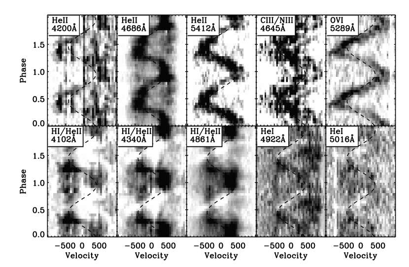
Figure 2: Trailed spectra of ten prominent lines in UY Vol. The He ii lines show clear S-wave patterns. The Bowen blend shows a broad S-wave feature with no narrow emission lines. The O vi line shows a clear S-wave with an amplitude $K_{\rm em}=710$km/s. Trailed spectra for He i and blended H i/He ii lines reveal phase-dependent absorption. Sine waves are over-plotted to guide the eye, with amplitude of 410 km/s and a phase offset of $\phi_{0}=0.3$.

Binning our 68 spectra by phase, we create trailed spectra for each observed line, and plot those in Figure 2. We observe clear modulation of the line flux with phase in all lines, and S-wave patterns emerge in several cases. The S-waves in the He ii trailed spectra have a hooked shape with a sharp $dv/d\phi$ at $\phi<0.5$ and a smoother change for $\phi>0.5$. Emission is also relatively fainter at $\phi\sim 0.75$. The O vi and Bowen blend lines also show clear S-waves. The O vi line shows higher emission velocity than H and He (710 km/s vs. 403 km/s), indicating either a location deeper inside the accretion disk or high velocity disk overflow. Interestingly, in examining the LMXB 2A 1822–371, Casares et al. (2003) find that the O vi $\lambda$3811 emission they observe has a radial velocity amplitude significantly larger than that of H/He components.

Both He i and H i/He ii blends show characteristic absorption in the trailed spectra making it difficult to identify a clear S-wave pattern. In He i lines, absorption occurs consistently at $0.7<\phi<0.9$. This is the same phase range at which X-ray dips are seen, suggesting the absorption may also be associated with the stream and its impact point. All lines showing S-waves have phasing consistent with emission originating in the accretion disk, either near the matter stream impact point or downstream of it.

3.3 The Doppler Corrected Spectrum

Muñoz-Darias et al. (2009) suggested that sharp components could be seen in the Bowen line profile if it was Doppler-corrected to match a companion star radial velocity semi-amplitude of $K_{\rm em}=300$ km/s, corresponding to a feature seen in their He ii Doppler tomogram. We also find that sharp components can be recovered by Doppler correction at approximately this velocity, but have not been able to reproduce corresponding features in a tomogram. One should be cautious in interpreting results of Doppler correction in isolation, as there could be multiple spurious combinations of phase and radial velocity that will produce small apparent peaks out of the noise.

We Doppler correct using the equation:

$$V(\phi)=\gamma+K_{\rm em}\sin 2\pi(\phi-\phi_{0}).$$ (1)

To quantify the Doppler correction procedure more rigorously, we investigated the full parameter space in phase (0–1 in steps of 0.02) and $K_{\rm em}$ (0–800 km/s in steps of 10 km/s). For each trial radial velocity curve we Doppler correct the Bowen profiles, and then cross-correlate them with a template consisting of one Gaussian matching the instrumental resolution for each N iii and C iii component. The individual strengths of the Gaussians were set to match those listed by McClintock et al. (1975) with the overall strength of nitrogen and carbon emission adjusted to best match our data. Using a cross-correlation in this way should favor finding specific patterns of lines matching the Bowen blend wavelengths rather than random peaks in the data, and should also result in a single dominant peak for a good match, rather than the multiple peaks present in the corrected line profiles.

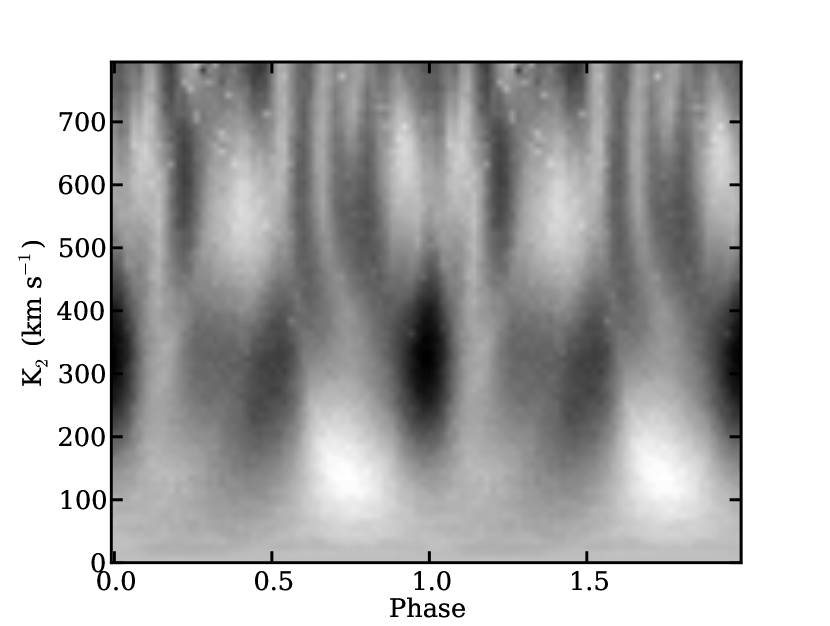
Figure 3: The strength of the residual cross-correlation peak after subtraction of the broad component of the correlation corresponding to the disk. A phase of 0 or 1 corresponds to a radial velocity curves in phase with the motion of the donor star.

After this procedure we find that the dominant feature in all of the cross-correlation functions is a broad peak corresponding to the broad emission associated with the disk. For phases near to zero and $K_{\rm em}$ near 300 km/s, a sharp peak is superposed on the broad maximum. To quantify the strength of this fit, we subtract a Gaussian fit to the broad maximum and then measure the height of the residual central peak. We show the strength of this peak as a function of the trial phases and $K_{\rm em}$ values in Figure 3.

We see that the strongest feature is seen in phase with the motion of the donor star. The peak is at a phase of $0.98$. We estimate $K_{\rm em}=329\pm 26$ km/s with the 1 $\sigma$ uncertainty derived from a bootstrap Monte Carlo simulation of our data analysis procedure. The velocity found is consistent with that of Muñoz-Darias et al. (2009) and the values determined from the quiescent He i tomograms of Bassa et al. (2009) and Ratti et al. (2012). In Figure 4, we show the Doppler corrected spectrum of UY Vol around the $\lambda$4686 and 5412 He ii lines using the value $K_{\rm em}=329$ km/s and $\gamma=70$ km/s. We adopt the latter throughout this work for consistency with (Muñoz-Darias et al., 2009); we find a consistent value from our O vi line.

While the Doppler corrected spectrum, shown in Figure 4 shows reasonable centering around the line centers, we do not see the strong narrow line emission in He ii. We observe at most a very small contribution to the He ii line from the companion star unlike Muñoz-Darias et al. (2009). Cornelisse et al. (2008) summarize a survey of 10 LMXBs, all of which show He ii emission that is not localized. However, many of these sources show H i in absorption. Both GX 9+9 and 2A 1822-371 show average spectra with H i in absorption (Casares et al., 2003; Cornelisse et al., 2007b, 2008). All of our blended H/He lines show a dual-peaked shape when Doppler corrected, with one peak strongly centered near the He ii emission and decreased emission near H i.

3.4 Tomograms

We next utilize the continuum subtracted spectra to perform Doppler tomography, first rebinning the data to a constant velocity scale of 30 km/s/pix. We then create tomograms using doppler (Marsh, 2005) which utilizes a combined maximum entropy and chi-square minimization technique. In all cases, the entropy is measured relative to a Gaussian blur default, meaning entropy is insensitive to large scale variations. We generate tomograms extending $\pm 1000$ km/s around the line center.

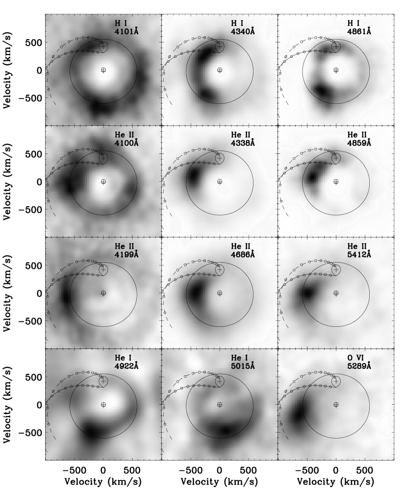
Figure 5: Doppler tomograms of identified lines. The components for the H i and He ii lines are deblended and shown separately.

We use only the 49 spectra for which the source is out of eclipse. The maps, shown in Figure 5, include model locations for the primary, secondary, matter stream, and L1 point for a 1.5 $M_{\odot}$ neutron star and an 0.1 M_⊙ donor (see Section 4.3). The bulk of the line emission emanates from the accretion disk, especially downstream of the matter impact point, with no definitive contribution from the donor star. We were not able to reconstruct a tomogram of the Bowen blend. The weak narrow line emission and the volume of contributing components resulted in poor maps.

In the top two rows of Figure 5, we show tomograms of our three H i/He ii lines. We used doppler to deblend the H/He contributions, and find that while the H i contribution is distributed throughout the disk, the He ii contribution is concentrated just downstream of the matter impact point. The location of the deblended He ii emission is consistent with that seen in the isolated He ii lines.

Using VLT data taken in 2003, Pearson et al. (2006) find He ii emission in $\lambda$4686, 5412 is brightest significantly closer to the matter stream and assumed location of the secondary. In both lines, Pearson et al. (2006) observe concentrated emission with $V_{Y}>0$ km/s. Our data very consistently shows $V_{Y}\sim 0$ km/s. Our data do not show the matter stream emission observed by Muñoz-Darias et al. (2009). Their data do show some emission features at negative $V_{Y}$. Since their data were taken one month prior to ours, this precludes the existence of a concentrated source of He ii emission migrating along the streaming disk.

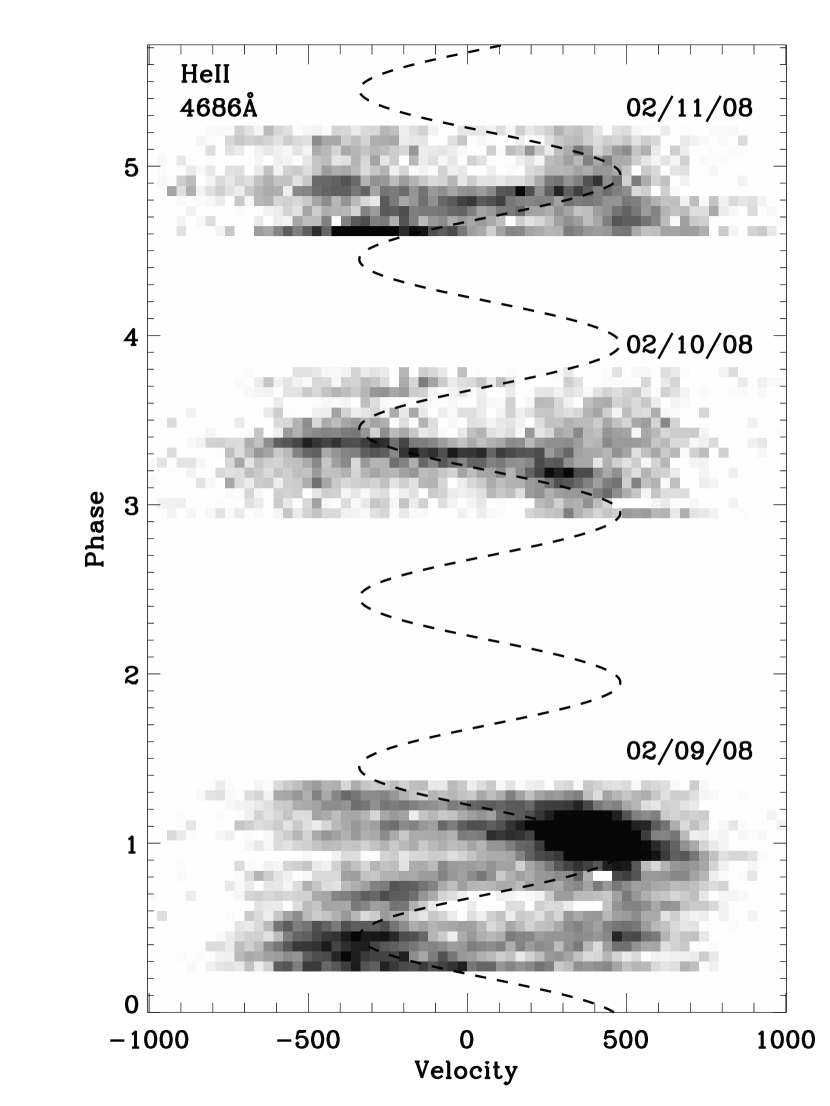
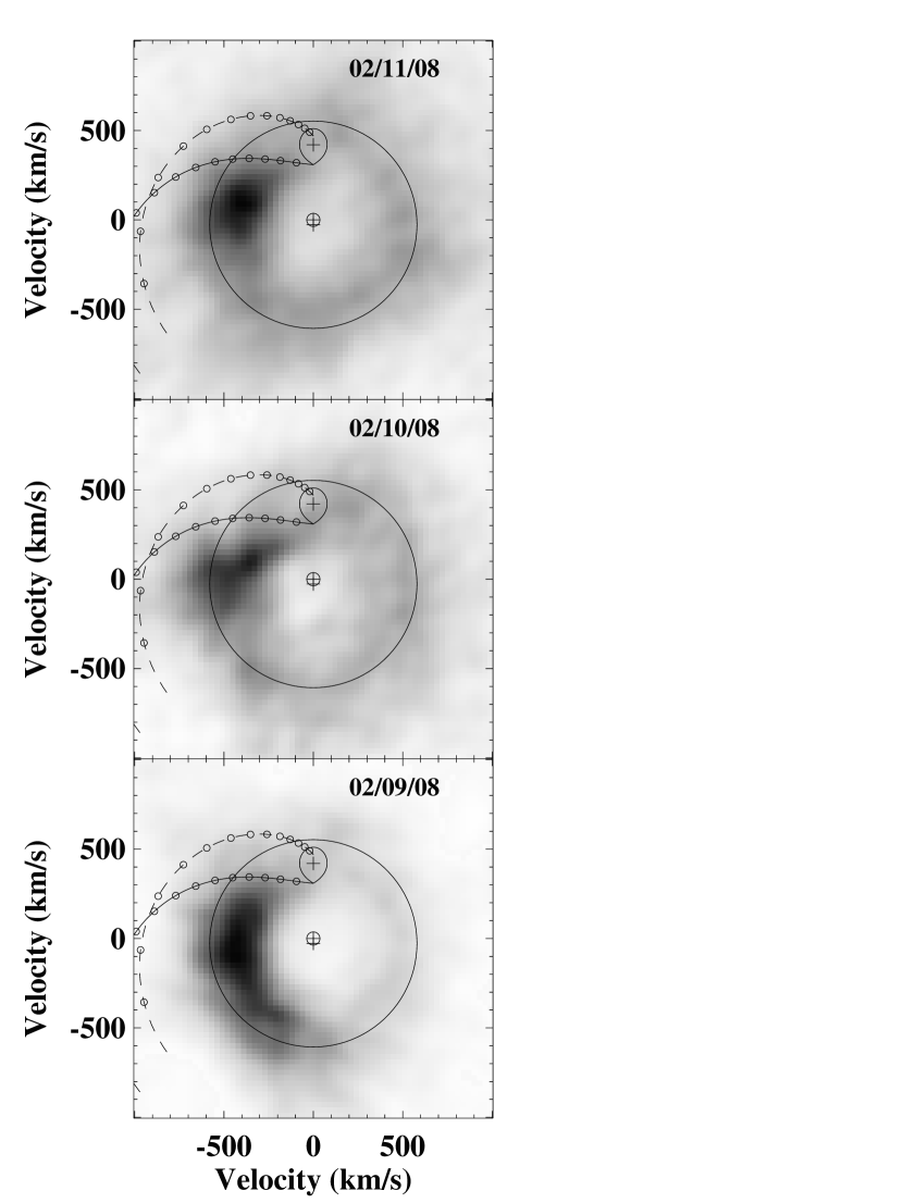
Figure 6: Night-by-night tomograms of He ii 4686. Note, the tomograms for 2/10 and 2/11 are shown at a fractional gray-scale relative to the 2/9 for clarity. They only achieve 50% of the signal. This is apparent by the relative peaks in the trailed spectra.

Because our data set covers multiple orbits, we were able to group our spectra and characterize the changes in the tomogram on a timescale of days. In Figure 6, we show the trailed spectra and tomograms for three consecutive days for which we had sufficient orbital coverage. On February 9, the emission in the trailed spectra is notably brighter and the peaks broader. In the tomogram, this corresponds to emission concentrated just downstream of the matter impact point with a large spread of emission along the lower left tomogram. The next evening, the peaks in the trailed spectra are notably narrower and the corresponding tomogram emission is more compact. On February 10, the emission disperses toward the upper right and on February 11, the emission is most concentrated. These variations in morphology also appear in the modulation maps (see below). Given how rapidly the centroid and morphology of He ii emission can change from epoch to epoch, it is unlikely that emission features in the tomogram associated with stream-disk impact region can be used to constrain the mass ratio reliably as attempted by Pearson et al. (2006).

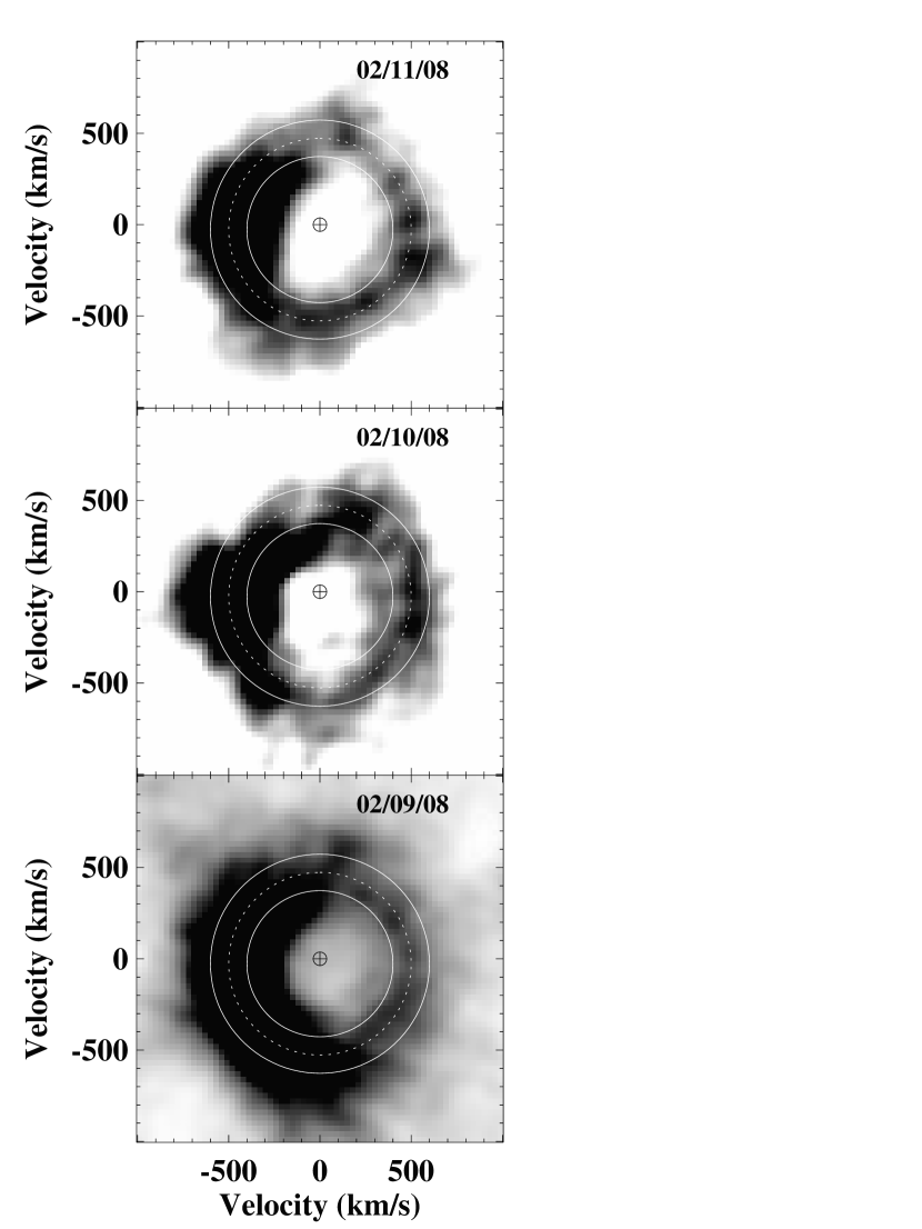
Figure 7: Night-by-night tomograms of He ii 4686 as for Figure 6. The gray-scale has now been adjusted individually to maximize visibility of the disk on the right hand side of the tomogram. The plotted circles correspond to disk velocities of 400, 500, and 600 km s^-1.

Our He ii 4686 Å maps do rather consistently define the accretion disk emission, and this potentially provides an alternative constraint on the system parameters. We show the same night-by-night tomograms in Figure 7, with the gray-scale adjusted to maximize visibility of the disk on the right hand side of the tomogram. We will concentrate on this region as it should not be distorted by the changes seen in the stream-impact/bulge region that vary from night-to-night. Instead the kinematics of the right hand side of the maps are very stable and define a circular ring quite well. The projected disk velocity indicated by the data is 500 km/s, and is well bounded by rings at 400 and 600 km/s. We will discuss the implications of interpreting this as a Keplerian disk velocity in Section 4.3.

In the last row of Figure 5, we see that He i emits more strongly in a different region of the disk to He ii, separated by about 0.25 in phase. It is possible that the He ii gets ionized near the matter impact point and is able to later recombine and form He i downstream.

The O vi emission is fairly concentrated, suggesting temperature conditions unique to O vi excitation at this point in the disk. Pearson et al. (2006) observe O v emission in the UV. As with our O vi observations, their O v observations do not occur along the the ballistic stream or at Keplerian velocity, however, it is consistent with a location downstream of the impact or the stream overflow (Pearson et al., 2006). The high velocity of the O vi emission observed in the tomogram is expected from the fact that the S-wave seen in our O vi trailed spectrum had a higher amplitude than that of the H/He lines.

The Doppler tomograms begin to form a consistent picture of the ionization structure of the disk. He ii is observed in the ionized disk bulge, predominantly on the left of the tomogram at negative $V_{X}$ and low $V_{Y}$. While we do observe some variance in the central location, we can say that we do not observe He ii emission from the donor star. We also know that the prominent He ii emission occurs downstream of the matter impact point. He i is absent from the ionized disk bulge. It occurs most prominently in the lower part of the tomogram at negative $V_{Y}$, along the flow of the disk stream. As it occurs on the opposite side of the disk from the matter stream, it is probable that the temperature conditions in the disk are more amicable to the recombination of He ii. The O vi emission, in contrast, may be tracing a higher ionization region inside the disk.

3.5 Modulation Maps

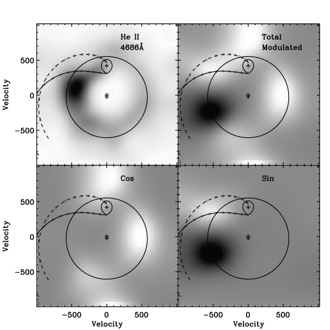
Figure 8: Modulation maps of the He ii $\lambda$4686 line. Starting at the upper left and going clockwise, the panels are (1) the average non-modulating emission, (2) the total modulated emission ($I_{sin}+I_{cos}$), (3) the $I_{sin}$ component of the modulated emission, and (4) the $I_{cos}$ component of the modulated emission. The modulation maps are shown at a fractional gray-scale of $\pm 6$% of the average, non-modulating emission.

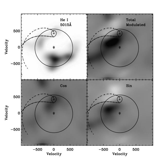
Figure 9: Modulation maps of the He i $\lambda$ 5015 line. The panels are as described in 8. The fractional gray-scale employed here is $\pm 35$% of the average non-modulating emission.

Modulation mapping is an extension of Doppler tomography that maps sources varying harmonically as a function of the orbital period (Steeghs, 2003). Periodic absorption, disk flickering, and varying visibility of the emission region all contribute to features in the modulation map. Thus, we must go back to the trailed spectra for a more accurate interpretation. At present, the modulation mapping code does not account for eclipsing, so we use only 49 of the 68 spectra for which the source was out of eclipse. Also, since the code does not deblend lines, we focus our study on isolated lines. Although modulation mapping works best with flux calibrated spectra, we did not have a comparison star on the slit for relative flux calibration. We assume that there is no significant continuum flux variation night to night and create modulation maps of all identified lines and plot two representative samples in Figures 8-9. Modulation mapping considers a line source modulating harmonically with flux as a function of orbital phase, such that $f(\phi)=I_{avg}+I_{cos}\cos(2\pi\phi)+I_{sin}\sin(2\pi\phi).$ The modulation maps show the average, non-varying line flux ($I_{avg}$) as well as the total modulated emission $(I_{sin}+I_{cos}$), and the individual sine and cosine emission maps. Because the modulated emission is often small relative to the average emission, the maps are shown on a fractional gray-scale relative to the average emission. Note that $I_{sin}$ and $I_{cos}$ can have positive or negative amplitudes and so their combination can model all phasings of the light curve.

For the $\lambda 4686$ He ii line, the modulated emission contributes less than 6% of the average emission. Figure 8 shows maps of the He ii $\lambda 4686$ line. As with the Doppler tomogram, we observe the classic disk structure in emission, and concentrated emission just downstream of the stream impact point. Modulated emission is dominated by the sine term and appears most strongly downstream of the impact point. This corresponds to the region where the night-to-night tomograms differ most (see Fig. 6). This modulated component would make our line emission appear brighter at $\phi\sim 0.25$ and fainter at $\phi\sim 0.75$. In the trailed spectrum, this is observed as a relative brightening in the S-wave near the peak radial velocity. A negative amplitude modulation appears in the cosine map, bordering the side of the disk farthest from impact. This would make our emission fainter at $\phi\sim 0$ and brighter at $\phi\sim 0.5$. In the trailed spectrum, this appears as increased emission at $\phi\sim 0.5$ in anti-phase with the S-wave amplitude. The modulating component may correspond to the irradiated inner edge of the stream bulge.

The split structure of the He i $\lambda 5015$ emission is readily apparent in the modulation map shown in Figure 9. Modulated emission here contributes up to 35% of the total flux. The sine term dominates the emission nearest the matter impact point. Very likely, this modulation does not represent varying visibility of an emission source, but rather the periodic absorption which is observed in the trailed spectra at $\phi\sim 0.75$. The non-modulated emission, $I_{avg}$ is strongest on the far side of the disk, where He ii is likely recombining.

The presence of modulating emission contributes to our emerging picture of the disk. We certainly confirm the presence of ionized He ii emission at or near the ionized disk bulge. The modulating feature in the sine map could represent the formation of optically thick clouds above and below the plane of the disk. These clouds are formed when the matter stream impacts the disk, and they are illuminated by X-rays from the disk. Since they are optically thick to X-rays, we would only observe these clouds at $\phi\sim 0.25$. These clouds may also be responsible for the periodic absorption in He i and H i and would be responsible for irregular X-ray dipping discovered by Parmar et al. (1986).

4 Discussion

4.1 Accretion disk structure

While Doppler tomography has long been used to interpret the accretion disk structure, we must be cautious not to over interpret certain aspects, as we have shown that prominent emission region morphology can vary between orbits. Our tomograms of He ii $\lambda$4686 and 5412 look different than those of Pearson et al. (2006) and Muñoz-Darias et al. (2009), but this is likely reflective of the disk evolving between epochs.

Pearson et al. (2006) attempted to constrain the mass ratio of UY Vol by studying emission from the matter stream as observed in their tomograms for He ii $\lambda$4686. Our observation of the same line does not show prominent emission from the matter impact point, but rather, some point on the disk downstream of the matter impact point. At best, our H i maps show some emission coincident with the velocities expected for the matter stream, and He ii is observed further downstream on the left side of the disk. The presence of He i emission in the lower part of the disk suggests the ionized He ii is recombining as it moves around the disk.

Neither Pearson et al. (2006) nor this work confirm the concentrated He ii emission coincident with the location of the donor star reported by Muñoz-Darias et al. (2009). While the morphology of prominent disk emission is expected to change rapidly, emission from the donor star should be more consistent. It is possible that the relative brightness of narrow emission from the donor compared to the disk made it unobservable at other epochs. We note that the He ii emission associated with the donor star by Muñoz-Darias et al. (2009) is part of a complex extending to negative $V_{x}$ in their maps, and roughly parallelling the stream trajectory. It is then also possible the the He ii seen at $V_{x}=0$ by Muñoz-Darias et al. (2009) originated from the beginning of the matter stream rather than the donor star itself, although it is unclear how He ii emission is produced in this region that should be shielded from direct irradiation by the disk rim.

As we must already use caution when comparing tomograms of the same source from different epochs, so too we must cautiously approach how we compare the tomograms of UY Vol to other LMXBs. In examining the source GX 9+9, Cornelisse et al. (2007b) observe prominent He ii emission in the lower left quadrant of their tomograms, where UY Vol shows more prominent He i. Hynes et al. (2001) find a similar emission structure for He ii in Doppler maps of XTE J2123-058. Both authors draw comparisons between these sources and SW Sex cataclysmic variables. The ionization structure of the emission source suggests a matter stream not connected with the accretion disk, that is either overflowing the disk or being propelled away (Hynes et al., 2001; Cornelisse et al., 2007b, and references therein).

In UY Vol, the six He ii lines for which we create tomograms show emission most concentrated at $V_{Y}\sim 0$, but the $V_{X}$ velocities occasionally suggest that while most emission is consistent with the Keplerian velocity of the outer edge of disk, some may be sub-Keplerian representing a similar overflow.

Casares et al. (2003) performed a study of the LMXB 2A 1822-371. Their map of He i $\lambda$4471 places the He i absorber on the leading side of companion’s Roche lobe or over the gas stream. It is not surprising that their He i maps are remarkably different than ours since they observe He i in absorption whereas UY Vol shows it in emission. Like UY Vol, 2A 1822-371 shows oxygen emission. Casares et al. (2003) observe O vi 3811 Å clearly in the post-shock region between the matter stream and the disk. This is in a very different location than that observed for UY Vol. Our O vi emission emanates downstream of the matter impact point, at a high velocity, suggesting it occurs either deeper within the disk or in a region of high-velocity disk overflow. It is worth nothing that 2A 1822-371 is also at a higher inclination and likely higher mass accretion rate than UY Vol, thus the direct stream impact may be more excited.

In summary, while UY Vol does not show the abundance of He i absorbers seen in 2A 1822-371, it does seem to show similar ionized emission in the disk and possible high-velocity and sub-Keplerian disk overflows as seen in other LMXBs. Interestingly, in UY Vol, we observe He i emission as part of the accretion disk structure, which may give us some insight to the relative mass accretion rate and disk temperature as compared to other LMXBs.

4.2 Abundances

We find that the C iii emission in the Doppler corrected Bowen blend profile in Figure 4 is of comparable strength to N iii. This can be compared to Sco X-1 (Steeghs & Casares, 2002), 2A 1822–371 (Casares et al., 2003), 4U 1636–536 (Casares et al., 2006), LMC X-2 (Cornelisse et al., 2007a), and Aql X-1 (Cornelisse et al., 2007c) where N iii is dominant, 4U 1735—444, (Casares et al., 2006) where C iii and N iii are of comparable strength, and GX 9+9 (Cornelisse et al., 2007b) where C iii dominates. Thus the C iii:N iii ratio in UY Vol is among the higher values seen among neutron star LMXBs, suggesting that the carbon abundance is at least normal, if not enhanced. We should be wary of over-interpreting the ratio, however, as it does depend on physical conditions as well as abundances. This is illustrated by the diversity of Bowen blend structures seen in GX 339–4 (Hynes et al., 2003).

As discussed in the case of GX 9+9, the strong C iii rules out substantial CNO processing of the accreted material since this would result in a pronounced deficit of carbon relative to nitrogen. The effects of CNO processing on LMXB spectra are even more pronounced in the far-UV, where the normally dominant C iv line can become completely undetectable, as in the case of the black hole system XTE J1118+480 (Haswell et al., 2002). In UY Vol, on the other hand, the far-UV spectrum is typical with a very strong C iv line (Pearson et al., 2006).

4.3 System parameters

There have now been four independent detections of features that appear to be associated with the companion star in UY Vol, spanning four different emission lines and both outburst and quiescence. In outburst we find $K_{\rm em}=329\pm 26$ km s^-1 in the Bowen blend, and Muñoz-Darias et al. (2009) obtain $K_{\rm em}=300\pm 10$ km s^-1 from He ii. In quiescence Bassa et al. (2009) obtain $345\pm 5$ km s^-1 in He i and $410\pm 5$ km s^-1 in H$\alpha$, while Ratti et al. (2012) find $308.5\pm 3.4$ km s^-1 from a weighted average of H$\beta$ and H$\gamma$. There is some spread in the deduced values, but there is also a striking congruence between them with emission from the companion star apparently spanning at least the range in velocity of 300–400 km s^-1, with different average velocities seen at different times and in different emission lines. This provides more information than a single detection, as discussed by Bassa et al. (2009), but also confuses interpretation as the ‘K correction’ from the observed $K_{\rm em}$ to the true $K_{2}$ value (Muñoz-Darias et al., 2005) cannot be single valued. Part of the variation can be accounted for with time-dependent variations in the disk shielding angle, $\alpha$, which are included in the models of Muñoz-Darias et al. (2005) but the Bassa et al. (2009) measurement of different $K_{\rm em}$ values simultaneously in H$\alpha$ and He i must indicate different patterns of emission across the donor star.

These limitations notwithstanding, we can attempt to constrain the masses of the binary components using this information. In some respects we follow the discussion of Muñoz-Darias et al. (2009) and Bassa et al. (2009), although we present the constraints more directly in $M_{2}$ vs. $M_{1}$ space in Figure 10. The first constraint is that the $K_{2}$ value must be greater than all measured $K_{\rm em}$. The H$\alpha$ detection is most constraining in this respect, requiring $K_{2}\gtrsim 405$ km s^-1. We show this constraint in Figure 10 as curve 1a which provides a lower limit on $M_{1}$ as a function of $M_{2}$. We can go beyond this limit if we assume that the emission originates in excitation by direct emission from near the compact object since the pole of the companion star itself (corresponding to $K_{\rm em}=K_{2}$) is shielded by the curve of the donor star’s surface. A tighter constraint is that $K_{\rm em}$ is less than the velocity at the tangent point, where rays from the compact object are tangential to the stellar surface. We show this constraint as curve 1b.

While there is uncertainty in the actual emission pattern over the donor star, the center of light must be between the L₁ point and the tangent point, so we also require that $K_{\rm L_{1}}$ be less than the smallest measured $K_{\rm em}$, i.e.  $K_{\rm L_{1}}\lesssim 310$ km s^-1. This constraint is shown as curve 2 in Figure 10 and this sets an upper limit on $M_{1}$ as a function of $M_{2}$. If $M_{1}$ lies above this line then the mass ratio of the system is small and the donor is consequently too small to be consistent with the range of velocities seen by different groups at different times.

These constraints together define a band in $M_{1}-M_{2}$ space that becomes increasingly narrow for small mass ratios. This argument (using curves 1a and 2) is essentially that used by Bassa et al. (2009) to constrain $0.075<q<0.105$ ($0.1<M_{2}<0.15$) for the specific case of a 1.4 _⊙ neutron star. This case is barely consistent with these constraints and requires an unusually extreme mass ratio and a very low-mass donor. Limiting emission to the tangent point rather than the pole (the band defined by curves 1b and 2) virtually eliminates a 1.4 _⊙ neutron star from consideration.

A 1.4 M_⊙ neutron star is often assumed in LMXBs. There is some support for this in the observed tight distribution of masses of radio pulsars in binaries, of $1.35\pm 0.04$ M_⊙ (Thorsett & Chakrabarty, 1999). This tight distribution presumably reflects the distribution in birth masses, however, whereas neutron stars in LMXBs are accreting and so are likely to be of higher mass. Indeed, we do see rather larger masses where we can measure them in milli-second pulsars which are believed to be the descendants of LMXBs (Demorest et al., 2010). Moving on to the companion star, the default assumption is often that it is a main-sequence star, or at least lies close to a main-sequence mass-radius relation. While under-massive mass donors are seen in some LMXBs, a main-sequence donor is still a reasonable starting point in the absence of other evidence for a more evolved status. Such other evidence can sometimes be very strong, for example, in abundance anomalies indicating that the donor has experienced a prior period of CNO burning (e.g. XTE J1118+480; Haswell et al. 2002). In the case of UY Vol, however, as discussed in Section 4.2, it appears that the carbon abundance is at least normal, if not enhanced. If we follow the usual prescription for deducing the mass of a main-sequence donor in an interacting binary (Frank et al., 2002) we obtain $M_{2}=0.42$ M_⊙. This is based on very simplistic assumptions ($R/R_{\odot}=M/M_{\odot}$ on the lower main-sequence), and more realistic mass radius relations produce somewhat lower donor masses. By way of example, we show in Figure 10 the mass-radius relation of Patterson (1984) as curve 3. This favors masses around 0.37 M_⊙ for plausible neutron star masses.

We can now draw one quite strong conclusion from the dynamical evidence in Figure 10: if the donor star is on the main-sequence, then the neutron star is massive. If curve 1b is obeyed (i.e. quiescent H$\alpha$ emission is driven by direct irradiation from the neutron star or inner disk), then a main-sequence companion star requires a neutron star more massive than about 2 M_⊙. This case would actually agree quite well with the mass estimate of Özel (2006) of $2.1\pm 0.28$ M_⊙. Alternatively if we expect the neutron star to be closer to the canonical 1.4 M_⊙, then we require a significantly under-massive donor. In that case, we might expect to see evidence of CNO processing as in, for example, XTE J1118+480 (Haswell et al., 2002), and we clearly do not. In this case, however, the low mass may be a consequence of evaporation of an initially sub-Solar donor in a ‘Black-Widow-like’ scenario (Ratti et al., 2012) where no CNO processing has had timeto occur.

We have one final dynamical constraint that has not been included yet. We observe the peak disk emission in He ii around a projected Keplerian disk velocity of $V_{\rm kep}\sin i=500$ km s^-1, and it is quite well bounded by a range of 400–600 km s^-1. This turns out to be difficult to accommodate simultaneously with the dynamical constraints from the donor star. For a given pair of $M_{1},M_{2}$ values, the mass ratio and inclination are uniquely determined (via X-ray eclipses), and so the projected Keplerian velocity from the disk rim can be calculated. We assume the disk is tidally truncated at 0.9 $R_{\rm lobe}$ (Whitehurst & King, 1991), and refer to this velocity as $V{\rm kep,tidal}$. This should be the minimum allowed velocity in a Keplerian disk. We show in Figure 10 a final set of curves (4a–d) corresponding to the loci $V_{\rm kep,tidal}\sin i=400$, 500, 600, and 700 km s^-1 respectively. The 500 km s^-1 curve is not consistent with the dynamical constraints at all, and even 600 km s^-1 is only consistent with the lowest $M_{1}$ and $M_{2}$ values, and requires that the He ii emission be mildly sub-Keplerian. Accommodating a main-sequence donor would require that the He ii emission be sub-Keplerian by about 50 %. The dynamical constraints from the disk velocities thus favor relatively small masses, but we cannot robustly rule out higher masses since all plausible solutions require some degree of sub-Keplerian motion.

We note that there is a caveat to this last point. Somero et al. (2012) have recently reported a similar analysis of 2A 1822-371, where they find He ii emission with disk-like morphology, but sub-Keplerian velocity. In the case of 2A 1822-371 the parameters are better constrained, so this conclusion cannot be avoided. That object also appears to be accreting at a substantially higher rate that UY Vol, however, and with significant mass loss (Bayless et al., 2010; Burderi et al., 2010). Somero et al. (2012) argue that their He ii emission originates in a disk wind above the orbital plane. It is then quite likely that 2A 1822-371 is an anomaly, and that UY Vol (with lower mass transfer rate) should exhibit more normal disk emission.

5 Conclusions

We have examined optical spectroscopy of the LMXB UY Vol spanning several orbits and observing nights. Doppler tomography shows that the strongest line emission, seen most characteristically in He ii, originates in the vicinity of the disk rim downstream of the stream-impact point. This dominant component is observed to be quite variable in intensity and in how far around the disk it extends. The variations are seen both within a night, and from night-to-night. This component is superimposed on weaker, less variable emission from the accretion disk. The phasing of the variations is consistent with the He ii emission originating on the irradiated inner side of a disk bulge region. The higher excitation O VI line is seen at a higher velocity than He ii, suggesting some stream overflow. It quite closely resembles the O v line seen in the far-UV by Pearson et al. (2006) in its kinematic behavior.

Careful examination of the Bowen blend reveals N iii and C iii components moving in phase with the companion star. These are best seen by Doppler correcting the line profiles using radial velocity curves and they are maximized for $K_{\rm em}=329\pm 26$ km/s, consistent with independent measurements of $K_{\rm em}$ by Muñoz-Darias et al. (2009), Bassa et al. (2009), and Ratti et al. (2012). Combining these dynamical constraints with the inferred disk velocities from our Doppler tomograms, we favor a neutron star close to the canonical mass, $M_{1}\sim 1.5$ M_⊙ and a very low mass donor star, with $M_{2}\sim 0.1$ M_⊙, in spite of the lack of evidence for CNO processing. Even this solution requires that the peak disk-emission be mildly sub-Keplerian. Higher masses are disfavored but cannot be securely ruled out. A main-sequence donor star ($M_{2}\simeq 0.37$ M_⊙) would require $M_{1}>2.0$ M_⊙ and peak disk emission at velocities 30 % lower than expected at the edge of the disk.

Figure 1: The average, continuum normalized spectrum of UY Vol. We identify a variety of H/He lines with double-peak structures indicative of emission originating in the accretion disk. The He ii 4-9 falls on a chip gap. Measured line centers are listed in Table 2.

Figure 4: We create a Doppler corrected spectrum using $K_{\rm em}=329$ km/s and $\gamma=70$ km/s. While we may tentatively identify narrow features in the Bowen blend, we do not observe strong narrow features in He ii. Note that He ii $\lambda$4542 occurs on a chip gap, so our Doppler reconstruction of that line is incomplete.

Figure 10: Dynamical constraints on the mass of the neutron star ($M_{1}$) and the companion star ($M_{2}$). The horizontal solid line corresponds to a canonical 1.4 _⊙ neutron star. The solid lines 1a and 1b are derived from the quiescent H$\alpha$ measurement of Bassa et al. (2009). The lower line, 1a is a lower boundary of allowed parameter space assuming only that $K_{2}>K_{\rm em}$. The higher line, 1b requires additionally that the H$\alpha$ emission originates in regions directly illuminated by the neutron star. The dashed line, 2, is obtained from the He ii measurement of Muñoz-Darias et al. (2009), assuming that $K_{\rm L_{1}}<K_{\rm em}$. The dot-dashed line 3 represents main-sequence donors that fill the companion star Roche lobe. Finally, the dotted lines are constraints imposed by our measurements of the disk velocity. Curves 4a–d respectively correspond to outer disk velocities of 400, 500, 600, and 700 km/s.

Table 1: Log of GMOS Observations

Date	Start Time (MJD)	End Time (MJD)	Start Phase	End Phase	Orbits
2008-02-09	54505.193	54505.370	0.269	0.398	1.11
2008-02-10	54506.103	54506.231	0.981	0.790	0.81
2008-02-11	54507.171	54507.337	0.650	0.728	1.04
2008-03-14	54539.019	54539.049	0.576	0.772	0.19

Table 2: IDENTIFIED LINES

Line	$\lambda_{air}$	$\lambda_{c}$ (Å)
H i 2-6	4101.734	4101.6 $\pm$ 0.6
He ii 4-12	4100.041
He ii 4-11	4199.832	4201. $\pm$ 2.
H i 2-5	4340.464	4340.8 $\pm$ 0.9
He ii 4-10	4338.671
He ii 4-9	4541.591	–
C iii	4647.4	4645.0 $\pm$ 0.8
	4650.3
	4651.5
N iii	4634.2
	4640.6
	4641.9
He  ii 3-4	4685.71	4686.3 $\pm$ 0.8
H i 2-4	4861.352	4861.4 $\pm$ 0.7
He  ii 4-8	4859.20
He i	4921.93	4922. $\pm$ 1
He i	5015.67	5015.3 $\pm$ 0.8
C/N/O blend	–	5133
O vi	5289.	5289. $\pm$ 1.
O vi	5290.	.
He  ii 4-7	5411.53	5412. $\pm$ 1.

Note. — Table of identified lines. The second column is the laboratory predicted central wavelength in air. The third column is the best estimate of the centroid as measured from the average spectra. Errors are estimated by creating two statistically independent spectra each summing over 34 of our nights. The $\lambda$4541 He ii line falls on a chip gap, so no center is measured. The feature visible at 5133Å is likely a blend of C/N/O.

References

- Bassa et al. (2009) Bassa, C. G., Jonker, P. G., Steeghs, D., & Torres, M. A. P. 2009, MNRAS, 399, 2055
- Bayless et al. (2010) Bayless, A. J., Robinson, E. L., Hynes, R. I., Ashcraft, T. A., & Cornell, M. E. 2010, ApJ, 709, 251
- Burderi et al. (2010) Burderi, L., di Salvo, T., Riggio, A., et al. 2010, A&A, 515, A44
- Casares et al. (2006) Casares, J., Cornelisse, R., Steeghs, D., Charles, P. A., Hynes, R. I., O’Brien, K., & Strohmayer, T. E. 2006, MNRAS, 373, 1235
- Casares et al. (2003) Casares, J., Steeghs, D., Hynes, R. I., Charles, P. A., & O’Brien, K. 2003, ApJ, 590, 1041
- Casares et al. (1995) Casares, J., Martin, A. C., Charles, P. A., Martin, E. L., Rebolo, R., Harlaftis, E. T., & Castro-Tirado, A. J. 1995, MNRAS, 276, L35
- Cornelisse et al. (2008) Cornelisse, R., Casares, J., Muñoz-Darias, T., Steeghs, D., Charles, P., Hynes, R., O’Brien, K., & Barnes, A. 2008, A Population Explosion: The Nature & Evolution of X-ray Binaries in Diverse Environments, 1010, 148
- Cornelisse et al. (2007a) Cornelisse, R., Steeghs, D., Casares, J., et al. 2007, MNRAS, 381, 194
- Cornelisse et al. (2007b) Cornelisse, R., Steeghs, D., Casares, J., Charles, P. A., Barnes, A. D., Hynes, R. I., & O’Brien, K. 2007, MNRAS, 380, 1219
- Cornelisse et al. (2007c) Cornelisse, R., Casares, J., Steeghs, D., et al. 2007, MNRAS, 375, 1463
- Cottam et al. (2002) Cottam, J., Paerels, F., & Mendez, M. 2002, Nature, 420, 51
- Cottam et al. (2008) Cottam, J., Paerels, F., Méndez, M., et al. 2008, ApJ, 672, 504
- Demorest et al. (2010) Demorest, P. B., Pennucci, T., Ransom, S. M., Roberts, M. S. E., & Hessels, J. W. T. 2010, Nature, 467, 1081
- Frank et al. (2002) Frank, J., King, A., & Raine, D. J. 2002, Accretion Power in Astrophysics, 3rd Edn., Cambridge University Press
- Gottwald et al. (1986) Gottwald, M., Haberl, F., Parmar, A. N., & White, N. E. 1986, ApJ, 308, 213
- Haswell et al. (2002) Haswell, C. A., Hynes, R. I., King, A. R., & Schenker, K. 2002, MNRAS, 332, 928
- Hook et al. (2004) Hook, I. M., Jørgensen, I., Allington-Smith, J. R., Davies, R. L., Metcalfe, N., Murowinski, R. G., & Crampton, D. 2004, PASP, 116, 425
- Hynes & Jones (2009) Hynes, R. I., & Jones, E. D. 2009, ApJ, 697, L14
- Hynes & Jones (2008) Hynes, R., & Jones, E. 2008, The Astronomer’s Telegram, 1816
- Hynes et al. (2006) Hynes, R. I., Horne, K., O’Brien, K., Haswell, C. A., Robinson, E. L., King, A. R., Charles, P. A., & Pearson, K. J. 2006, ApJ, 648, 1156
- Hynes et al. (2003) Hynes, R. I., Steeghs, D., Casares, J., Charles, P. A., & O’Brien, K. 2003, ApJ, 583, L95
- Hynes et al. (2001) Hynes, R. I., Charles, P. A., Haswell, C. A., Casares, J., Zurita, C., & Serra-Ricart, M. 2001, MNRAS, 324, 180
- Lattimer & Prakash (2007) Lattimer, J. M., & Prakash, M. 2007, Phys. Rep., 442, 109
- Lin et al. (2010) Lin, J., Özel, F., Chakrabarty, D., & Psaltis, D. 2010, ApJ, 723, 1053
- Marsh (2005) Marsh, T. R. 2005, Ap&SS, 296, 403
- McClintock et al. (1975) McClintock, J. E., Canizares, C. R., & Tarter, C. B. 1975, ApJ, 198, 641
- Muñoz-Darias et al. (2005) Muñoz-Darias, T., Casares, J., & Martínez-Pais, I. G. 2005, ApJ, 635, 502
- Muñoz-Darias et al. (2009) Muñoz-Darias, T., Casares, J., O’Brien, K., Steeghs, D., Martínez-Pais, I. G., Cornelisse, R., & Charles, P. A. 2009, MNRAS, 394, L136
- Özel (2006) Özel, F. 2006, Nature, 441, 1115
- Parmar et al. (1986) Parmar, A. N., White, N. E., Giommi, P., & Gottwald, M. 1986, ApJ, 308, 199
- Parmar et al. (1985) Parmar, A. N., Gottwald, M., Haberl, F., Giommi, P., & White, N. E. 1985, Recent Results on Cataclysmic Variables. The Importance of IUE and Exosat Results on Cataclysmic Variables and Low-Mass X-Ray Binaries, 236, 119
- Patterson (1984) Patterson, J. 1984, ApJS, 54, 443
- Pearson et al. (2006) Pearson, K. J., et al. 2006, ApJ, 648, 1169
- Ratti et al. (2012) Ratti, E. M., Steeghs, D. T. H., Jonker, P. G., et al. 2012, MNRAS, 420, 75
- Schmidtke et al. (2000) Schmidtke, P. C., Cowley, A. P., Taylor, V. A., Crampton, D., & Hutchings, J. B. 2000, AJ, 120, 935
- Somero et al. (2012) Somero, A., Hakala, P., Muhli, P., Charles, P., & Vilhu, O. 2012, A&A, in press (arXiv:1201.3461)
- Steeghs (2003) Steeghs, D. 2003, MNRAS, 344, 448
- Steeghs & Casares (2002) Steeghs, D., & Casares, J. 2002, ApJ, 568, 273
- Thorsett & Chakrabarty (1999) Thorsett, S. E., & Chakrabarty, D. 1999, ApJ, 512, 288
- Torres et al. (2008) Torres, M. A. P., Jonker, P. G., Steeghs, D., & Seth, A. C. 2008, The Astronomer’s Telegram, 1817
- Wade et al. (1985) Wade, R. A., Quintana, H., Horne, K., & Marsh, T. R. 1985, PASP, 97, 1092
- Whitehurst & King (1991) Whitehurst, R., & King, A. 1991, MNRAS, 249, 25
- Wolff et al. (2008) Wolff, M., Ray, P., Wood, K., & Wijnands, R. 2008, The Astronomer’s Telegram, 1812
- Wolff, Ray, & Wood (2008) Wolff, M. T., Ray, P. S., & Wood, K. S. 2008, The Astronomer’s Telegram, 1736
- Wolff et al. (2002) Wolff, M. T., Hertz, P., Wood, K. S., Ray, P. S., & Bandyopadhyay, R. M. 2002, ApJ, 575, 384