Cantor set zeros of one-dimensional Brownian motion minus Cantor function

Abstract.

In [ABPR] it was shown by Antunović, Burdzy, Peres, and Ruscher that a Cantor function added to one-dimensional Brownian motion has zeros in the middle $\alpha$-Cantor set, $\alpha\in(0,1)$, with positive probability if and only if $\alpha\neq 1/2$. We give a refined picture by considering a generalized version of middle $1/2$-Cantor sets. By allowing the middle $1/2$ intervals to vary in size around the value $1/2$ at each iteration step we will see that there is a big class of generalized Cantor functions such that if these are added to one-dimensional Brownian motion, there are no zeros lying in the corresponding Cantor set almost surely.

1. Introduction

Let $B(t)$ be standard one-dimensional Brownian motion with $B(0)=0$, let $C_{\alpha}$ be be a middle $\alpha$-Cantor set for $\alpha\in(0,1)$ on the interval $[1,2]$ and let $f_{\alpha}\colon[1,2]\to[0,1]$ be the corresponding Cantor function. For any function $g$ defined on some interval $I\subset\mathbb{R}^{+}$ denote by $\operatorname{\mathcal{Z}}(g)$ the set of zeros of $g$ in $(0,\infty)$.

Taylor and Watson (Example 3 in [TW]) showed that Brownian does not intersect the graph of the middle $1/2$-Cantor function restricted to the Cantor set, even though the projection of this set on the vertical axis is an interval. Surprisingly, the middle $1/2$-Cantor function is an exception in the following sense.

Theorem 1.1 ([ABPR]).

$\mathbb{P}(\operatorname{\mathcal{Z}}(B-f_{\alpha})\cap C_{\alpha}\neq\emptyset)>0$ holds if and only if $\alpha\neq 1/2$.

In the paper [ABPR] part of this result is used to prove that for every $\beta<1/2$ there is a $\beta$-Hölder continuous function $f\colon\mathbb{R}^{+}\to\mathbb{R}$ such that the set $\operatorname{\mathcal{Z}}(B-f)$ has isolated points with positive probability.

Theorem 1.1 is the main motivation of our present work. We investigate a more general class of Cantor functions defined in section 2. The $n$-th approximation of the middle $1/2$-Cantor function increases on some intervals of length $4^{-n}$ and is constant elsewhere. We now allow these intervals to vary in length for every iteration step meaning that for a positive, real sequence $(a_{n})$ the length of intervals where the function increases is $4^{-n}a_{n}^{2}$ at iteration level $n$. See Figure 1 for example. Theorems 3.1 and 3.3 give conditions for which of these generalized Cantor functions $f_{b}$ the process $B-f_{b}$ has zeros in the corresponding generalized Cantor set with positive probability or with probability $0$, respectively.

Other questions concerning path properties of Brownian motion with variable drift lying outside the Cameron-Martin space have been studied recently, e.g. in [ABPR], [APV], [PS] and [R12].

2. Generalized Cantor sets and generalized Cantor function

We now define a generalized Cantor set analogously to the standard Cantor set (see for instance section 3 of [ABPR]).

For a given positive, real sequence $(a_{n})$ we define a sequence $(b_{n})$ by $b_{n}:=(2^{-n}\cdot a_{n})^{2}$. For this sequence we define a corresponding Cantor-type set and denote it by $C_{b}$. Take a closed interval $I$ of length $b_{0}=a_{0}$. Let $\mathfrak{C}_{b_{1}}$ be the set consisting of two disjoint closed subintervals of $I$ of length $b_{1}$, the left one (for which the left endpoint coincides with the left endpoint of $I$) and the right one (for which the right endpoint coincides with the right endpoint of $I$). Now continue recursively, if $J\in\mathfrak{C}_{b_{n}}$, then include in the set $\mathfrak{C}_{b_{n+1}}$ its left and right closed subintervals of length $b_{n+1}$. We define the set $C_{b_{n}}$ as the union of all the intervals from $\mathfrak{C}_{b_{n}}$. For any $n$, the family $\mathfrak{C}_{b_{n}}$ is the set of all connected components of the set $C_{b_{n}}$. The generalized Cantor set is a compact set defined as $C_{b}=\bigcap_{n=1}^{\infty}C_{b_{n}}$.

Now we construct a Cantor-type function corresponding to the generalized Cantor set above. Define the function $f_{b_{1}}$ so that it has values $0$ and $1$ at the left and the right endpoint of the interval $I$, respectively, value $1/2$ on $I\backslash{C}_{b_{1}}$ and interpolate linearly on the intervals in $\mathfrak{C}_{b_{1}}$. Recursively, construct the function $f_{b_{n+1}}$ so that for every interval $J=[s,t]\in\mathfrak{C}_{b_{n}}$, the function $f_{b_{n+1}}$ agrees with $f_{b_{n}}$ at $s$ and $t$, it has value $(f_{b_{n}}(s)+f_{b_{n}}(t))/2$ on $J\backslash C_{b_{n+1}}$ and interpolate linearly on the intervals in $\mathfrak{C}_{b_{n+1}}$.

Figure 1. First three approximations of the generalized Cantor function on the interval $[1,2]$ (functions $f_{b_{n}}$ from the construction for $b_{1}=0.4$, $b_{2}=0.04$ and $b_{3}=0.01$, or $a_{1}=\sqrt{1.6}$, $a_{2}=\sqrt{0.64}$ and $a_{3}=0.8$, respectively. Approximations of the generalized Cantor set $C_{b}$ are drawn in bold).

The sequence of functions $(f_{b_{n}})$ converges uniformly on $I$. We define the generalized Cantor function $f_{b}$ as the limit $f_{b}=\lim_{n}f_{b_{n}}$. For any $n$ and all $m\leq n$ the functions $f_{b}$ and $f_{b_{n}}$ agree at the endpoints of intervals $J\in\mathfrak{C}_{b_{m}}$. See Figure 1 for an example.

Further, we fix an arbitrary small $\epsilon>0$ and require the sequence $(a_{n})$ to fulfill the condition $a_{n}^{2}-\frac{1}{2}a_{n+1}^{2}\geq\epsilon a_{n}^{2}$ (or equivalently $b_{n}-2b_{n+1}\geq\epsilon b_{n}$) for all $n$. Corollary 3.5 addresses the more general case of having a weaker condition $b_{n}-2b_{n+1}>0$ for all $n$. So we will only consider non-degenerate Cantor sets/ functions. Note that if the sequence $(a_{n})$ is monotone decreasing, then $a_{n}^{2}-\frac{1}{2}a_{n+1}^{2}\geq\frac{1}{2}a_{n}^{2}$ holds for all $n$.

For simplicity, we will assume the initial interval $I$ to be $[1,2]$, and we can extend the function $f_{b}$ to $\mathbb{R}^{+}$, for instance by value $0$ on $[0,1)$ and value $1$ on $(2,\infty)$.

3. Zeros in the generalized Cantor set

The following theorem gives a condition for which sequences $(b_{n})$ (or $(a_{n})$ respectively) $B-f_{b}$ has zeros in the generalized Cantor set with positive probability.

Theorem 3.1.

$\mathbb{P}(\operatorname{\mathcal{Z}}(B-f_{b})\cap C_{b}\neq\emptyset)>0$ holds if either
$\sum_{n=1}^{\infty}a_{n}<\infty$, or
$\sum_{n=1}^{\infty}\frac{1}{a_{n}}<\infty$.

Remarks 3.2.

(i) Note that for geometric series $(a_{n})$ the result was already shown in Theorem 1.1 (i.e. Theorem 1.3. of [ABPR]). For $a_{n}=\frac{1}{x^{n}}$ with some $x>1$ gives $b_{n}:=(2^{-n}\cdot\frac{1}{x^{n}})^{2}=(2x)^{-2n}$ which corresponds to $\alpha=1-\frac{1}{x}$ in Theorem 1.1. So for $\sum_{n=1}^{\infty}a_{n}<\infty$ Theorem 3.1 extends Theorem 1.1 for convergent series $(\sum a_{n})$ that increase slower than geometric series, for instance take $a_{n}=\frac{1}{n^{d}}$ with $d>1$.

(ii)The generalized Cantor function $f_{b}$ is not necessarily $\alpha$-Hölder continuous for some $\alpha\in(0,1)$. If the sequence $a_{n}$ fulfills that $-\log 2\cdot\frac{n}{\log a_{n}}$ converges to some $\sigma\in(0,1)$, then the corresponding generalized Cantor function is $\sigma$-Hölder continuous. For example, the generalized Cantor function corresponding to the sequence $(n^{-d})$ with $d>1$ does not satisfy a Hölder condition of any positive order.

To prove Theorem 3.1 we will use essentially the same method as in [ABPR].

Proof of Theorem 3.1.

For an interval $I=[r,s]\in\mathfrak{C}_{b_{n}}$, define $Z_{n}(I)$ as the event $B(s)\in[f_{b}(r),f_{b}(s)]$, and the random variable $Z_{b_{n}}=\sum_{I\in\mathfrak{C}_{b_{n}}}\mathbf{1}(Z_{n}(I))$, where $\mathbf{1}(Z_{n}(I))$ is the indicator function of the event $Z_{n}(I)$.

Note that, by simple bounds on the transition density of Brownian motion, there is a constant $c_{1}>0$, such that for any sequence $b_{n}:=(2^{-n}\cdot a_{n})^{2}$,

$$c_{1}2^{-n}\leq\mathbb{P}(Z_{n}(I))\leq 2^{-n}\ \text{ and }\ c_{1}\leq\mathbb{E}(Z_{b_{n}})\leq 1.$$ (1)

If the event $Z_{b_{n}}>0$ happens for infinitely many $n$’s, then we can find a sequence of intervals $I_{k}=[r_{k},s_{k}]\in\mathfrak{C}_{b_{n_{k}}}$, such that $f_{b}(r_{k})\leq B(s_{k})\leq f_{b}(s_{k})$, thus $|B(s_{k})-f_{b}(s_{k})|\leq 2^{-n_{k}}$. Since $s_{k}\in C_{b_{n_{k}}}$, the sequence $(s_{k})$ will have a subsequence converging to some $s\in C_{b}$, which satisfies $B(s)=f_{b}(s)$. Therefore

$$\mathbb{P}(\operatorname{\mathcal{Z}}(B-f_{b})\cap C_{b}\neq\emptyset)\geq\mathbb{P}(\limsup_{n\rightarrow\infty}\{Z_{b_{n}}>0\}).$$ (2)

To bound the probabilities $\mathbb{P}(Z_{b_{n}}>0)$ from below we apply the Paley-Zygmund inequality (see Lemma 3.23 in [MP]):

$$\mathbb{P}(Z_{b_{n}}>0)\geq(\mathbb{E}Z_{b_{n}})^{2}/\mathbb{E}(Z_{b_{n}}^{2}).$$

Therefore, we have to bound the second moment $\mathbb{E}(Z_{b_{n}}^{2})$ from above. We will use the following expression for the second moment

$$\mathbb{E}(Z_{b_{n}}^{2})=2\sum_{I,J\in\mathfrak{C}_{b_{n}}\atop I<J}\mathbb{P}(Z_{n}(I))\mathbb{P}(Z_{n}(J)\mid Z_{n}(I))+\mathbb{E}(Z_{b_{n}}),$$ (3)

where by $I<J$ we mean that the interval $I$ is located to the left of the interval $J$. Now we fix $n$ and intervals $I=[s_{1},t_{1}]$ and $J=[s_{2},t_{2}]$ from $\mathfrak{C}_{b_{n}}$, so that $I<J$. Let $x_{i}=f_{b}(s_{i})$ and $y_{i}=f_{b}(t_{i})$, for $i=1,2$. By the Markov property and the scaling property of Brownian motion, the process

$$\widetilde{B}(t)=(t_{2}-t_{1})^{-1/2}\Big{(}B(t_{1}+(t_{2}-t_{1})t)-B(t_{1})\Big{)},$$

is again a Brownian motion, independent of $\mathcal{F}_{t_{1}}$, and thus independent of the event $Z_{n}(I)\in\mathcal{F}_{t_{1}}$.

The event $Z_{n}(J)$ happens when $\widetilde{B}(1)\in\overline{J}$ for the interval $\overline{J}=[(t_{2}-t_{1})^{-1/2}(x_{2}-B(t_{1})),(t_{2}-t_{1})^{-1/2}(y_{2}-B(t_{1}))]$ of length $(t_{2}-t_{1})^{-1/2}2^{-n}$.

Figure 2. Events $Z_{n}(I)$ and $Z_{n}(J)$ (graph of Brownian motion intersects two bold vertical intervals).

Fix intervals $I^{0}$ and $J^{0}$ in $\mathfrak{C}_{b_{\ell+1}}$, which are contained in a single interval in $\mathfrak{C}_{b_{\ell}}$. Assume $I^{0}<J^{0}$ and label the intervals from $\mathfrak{C}_{b_{n}}$ contained in $I^{0}$ by $I_{1},\dots,I_{2^{n-\ell-1}}$, and those contained in $J^{0}$ by $J_{1},\dots,J_{2^{n-\ell-1}}$, so that $I_{i+1}<I_{i}$ and $J_{j}<J_{j+1}$. Set $I=I_{i}$ and $J=J_{j}$ for some $1\leq i,j\leq 2^{n-\ell-1}$, and define $x_{i}$, $y_{i}$, $\widetilde{B}$ and $\overline{J}$ as before. For $t_{2}-t_{1}$ we use the estimates $\epsilon b_{\ell}=\epsilon 2^{-2\ell}a_{\ell}^{2}\leq 2^{-2\ell}(a_{\ell}^{2}-\frac{1}{2}a_{\ell+1}^{2})=b_{\ell}-2b_{\ell+1}\leq t_{2}-t_{1}\leq b_{\ell}$. Conditional on $Z_{n}(I)$, the left endpoint of the interval $\overline{J}$ is at least $(x_{2}-y_{1})(t_{2}-t_{1})^{-1/2}$ and the right endpoint is at most $(y_{2}-x_{1})(t_{2}-t_{1})^{-1/2}$. Since $x_{2}-y_{1}=(i+j-2)2^{-n}$ and $y_{2}-x_{1}=(i+j)2^{-n}$ we have $\overline{J}\subset[(i+j-2)2^{-n}b_{\ell}^{-1/2},(i+j)2^{-n}(\epsilon b_{\ell})^{-1/2}]$. Because $\overline{J}$ has length at least $(b_{\ell})^{-1/2}2^{-n}=\frac{2^{\ell-n}}{a_{\ell}}$ and at most $(\epsilon b_{\ell})^{-1/2}2^{-n}=\frac{2^{\ell-n}}{\sqrt{\epsilon}a_{\ell}}$ we obtain

$$\mathbb{P}(Z_{n}(J_{j})\mid Z_{n}(I_{i})) =\mathbb{P}(\widetilde{B}(1)\in\overline{J}\mid Z_{n}(I))$$

$$\leq\frac{2^{\ell-n}}{\sqrt{2\pi\epsilon}a_{\ell}}\exp\Big{(}-\frac{1}{2}{((j+i-2)\frac{2^{\ell-n}}{a_{\ell}})^{2}}\Big{)}.$$

By summing over $1\leq i,j\leq 2^{n-\ell-1}$ it follows that

$$\sum_{1\leq i,j\leq 2^{n-\ell-1}}\mathbb{P}(Z_{n}(J_{j})\mid Z_{n}(I_{i}))\\ \leq 1+\frac{1}{\sqrt{2\pi\epsilon}}\sum_{k=1}^{\infty}(k+1)\frac{2^{\ell-n}}{a_{\ell}}\exp\Big{(}-\frac{1}{2}(\frac{2^{\ell-n}k}{a_{\ell}})^{2}\Big{)}$$ (4)

where we used the trivial bound for $i=j=1$. The sum on the right hand side can be written as

$$S(z)=z\sum_{k=1}^{\infty}(k+1)\exp(-(kz)^{2}/2),$$

for $z=\frac{2^{\ell-n}}{a_{\ell}}$. Since $\exp(-t^{2}/2)\leq\exp(-t+1/2)$, we get that

$$S(z)\leq e^{1/2}z\sum_{k\geq 1}(k+1)e^{-kz}=e^{1/2}z^{-1}\Big{(}\frac{z}{1-e^{-z}}\Big{)}^{2}(2e^{-z}-e^{-2z}).$$

Since $z\mapsto(\frac{z}{1-e^{-z}})^{2}(2e^{-z}-e^{-2z})$ is a bounded function on $\mathbb{R}^{+}$, it follows by (4) that for any fixed intervals $I^{0}$ and $J^{0}$ as above

$$\sum_{I,J\in\mathfrak{C}_{b_{n}}\atop I\subset I^{0},J\subset J^{0}}\mathbb{P}(Z_{n}(J)\mid Z_{n}(I))\leq 1+c_{2}\frac{a_{\ell}}{2^{\ell-n}},$$ (5)

for some constant $c_{2}>0$.

Therefore, summing the inequality in (5) over all intervals $I^{0}$ and $J^{0}$ and $\ell=0,\dots,n-1$, and using it together with (3) and (1), we have

$$\mathbb{E}(Z_{b_{n}}^{2})\leq 2^{-n+1}\sum_{\ell=0}^{n-1}\Big{(}2^{\ell}+2^{\ell}c_{2}\frac{a_{\ell}}{2^{\ell-n}}\Big{)}+1\leq 2\sum_{\ell=0}^{n}\Big{(}2^{-(n-\ell)}+c_{2}a_{\ell}\Big{)}.$$

Now we see that $\mathbb{E}(Z_{b_{n}}^{2})$ is bounded from above if $\sum_{n=1}^{\infty}a_{n}<\infty$. The lower bound in the second inequality in (1) and the Paley-Zygmund inequality imply that $\mathbb{P}(Z_{b_{n}}>0)\geq\mathbb{E}(Z_{b_{n}})^{2}/\mathbb{E}(Z_{b_{n}}^{2})$ is bounded from below and the claim follows for the first case of the theorem from (2).

Now for the second case pick intervals $I,J\in\mathfrak{C}_{b_{n}}$ such that $[s_{1},t_{1}]=I<J=[s_{2},t_{2}]$ and define $x_{i}$, $y_{i}$, $\widetilde{B}$ and $\overline{J}$ as before. By $\ell$ denote the largest integer such that both $I$ and $J$ are contained in a single interval from $\mathfrak{C}_{b_{\ell}}$. Assume that the event $Z_{n}(I)$ happens. We see that the endpoints of the interval $\overline{J}$ are satisfying that

$$\frac{x_{2}-B(t_{1})}{(t_{2}-t_{1})^{1/2}}\geq 0\ \text{ and }\ \frac{y_{2}-B(t_{1})}{(t_{2}-t_{1})^{1/2}}\leq 2^{-\ell}\cdot\sqrt{\frac{1}{\epsilon}}b_{\ell}^{-1/2}=\frac{1}{\sqrt{\epsilon}a_{\ell}}.$$

If $\frac{1}{a_{\ell}}$ is bounded, then the interval $\overline{J}$ is contained in a compact interval, which does not depend on the choice of $n$, $\ell$, $I$ or $J$. Using this and the fact that the length of $\overline{J}$ is bounded with $(b_{\ell})^{-1/2}2^{-n}\leq|\overline{J}|\leq(\epsilon b_{\ell})^{-1/2}2^{-n}$, we get that for some positive constants $c_{3}$ and $c_{4}$ we have

$$c_{3}(b_{\ell})^{-1/2}2^{-n}\leq\mathbb{P}(Z_{n}(J)\mid Z_{n}(I))=\mathbb{P}(\widetilde{B}(1)\in\overline{J}\mid Z_{n}(I))\leq c_{4}(\epsilon b_{\ell})^{-1/2}2^{-n}.$$ (6)

Substituting (6) and the upper bounds from (1) into (3), and summing over all intervals $I$ and $J$, we obtain

$$\mathbb{E}(Z_{b_{n}}^{2})\leq 1+2^{-n+1}\sum_{\ell=0}^{n-1}2^{\ell}2^{2(n-\ell-1)}c_{4}(\epsilon b_{\ell})^{-1/2}2^{-n}=1+c_{5}\sum_{\ell=0}^{n-1}\frac{1}{a_{\ell}}$$

for some positive constant $c_{5}$. We see that if $\sum_{n=1}^{\infty}\frac{1}{a_{n}}<\infty$, then $\mathbb{E}(Z_{b_{n}}^{2})$ is bounded from above by a constant not depending on $n$, and the claim follows.

∎

The following theorem gives a condition for which sequences $(b_{n})$ (or $(a_{n})$ respectively) $B-f_{b}$ has no zeros in the generalized Cantor set almost surely.

Theorem 3.3.

(i) If there is a sequence $(c_{n})$ with $\sum_{n=1}^{\infty}c_{n}=\infty$ and a fixed but arbitrary small $\delta>0$ and an $n_{0}>0$ such that for all $n\geq n_{0}$

$$\frac{1}{c_{n}}\geq a_{n}\geq\sqrt{\frac{1}{(8-\delta)\epsilon\ln{\frac{1}{c_{n}}}}},$$ (7)

then $\mathbb{P}(\operatorname{\mathcal{Z}}(B-f_{b})\cap C_{b}\neq\emptyset)=0$.

(ii) If $\sum_{\ell=1}^{n}\frac{1}{a_{\ell}}\rightarrow\infty$ for $n\rightarrow\infty$ and if there is a constant $C>0$ such that $\sum_{\ell=1}^{n}\frac{1}{a_{\ell}}\leq C\log n$ for all $n>0$, then $\mathbb{P}(\operatorname{\mathcal{Z}}(B-f_{b})\cap C_{b}\neq\emptyset)=0$.

Examples 3.4.

The sequence $(a_{n})$ defined by $a_{n}=\sqrt{\frac{1}{\ln{n}}}$ fulfills the conditions of the Theorem 3.3(i) (to see that choose $c_{n}=\frac{1}{n}$) and the sequence $(a_{n})$ defined by $a_{n}=n$ fulfills the conditions of the Theorem 3.3(ii).

By Theorem 3.3(i) also applies to sequences $(a_{n})$ where every element of the sequence is chosen from a fixed finite set of a numbers. Therefore, we see that $\mathbb{P}(\operatorname{\mathcal{Z}}(B-f_{b})\cap C_{b}\neq\emptyset)=0$ holds for all these sequences.

Note that, if two sequences $(a_{n})$ and $(a^{\prime}_{n})$ only differ by finitely many numbers, and if one of the sequences fulfills the conditions of one of the Theorems 3.1 or 3.3, then the other sequence fulfills the conditions of the same theorem.

Proof of Theorem 3.3.

For an interval $I\in\mathfrak{C}_{b_{n}}$, define $Y_{n}(I)$ as the event that Brownian motion hits the graph of $f_{b_{n}}$ on the interval $I$, that is a diagonal of the rectangle $I\times f_{b_{n}}(I)$, and the random variable $Y_{b_{n}}=\sum_{I\in\mathfrak{C}_{b_{n}}}\mathbf{1}(Y_{n}(I))$.

For an interval $I=[x,y]\in\mathfrak{C}_{b_{n}}$ define $R$ to be the corresponding rectangle $I\times f_{b}(I)$ and let $R_{1}$ be the triangle with the vertices $(x,f_{b}(x))$, $(y,f_{b}(y))$ and $(x,f_{b}(x)+2^{-n})$ (so it is the upper left triangle of $R$ with respect to the diagonal of $R$) and $R_{2}=R\backslash R_{1}$ is the lower right triangle part of $R$.

Fix an $n>0$ and let $C$ be the event that $B-f_{b_{n}}$ has a zero that is contained in $\mathfrak{C}_{b_{n}}$. Define $\overline{R}$ to be the event that $B-f_{b}$ has a zero that is contained in $\mathfrak{C}_{b}$ and the corresponding intersection point (by definition it is contained in a rectangle $R$ of described form) of the graph of Brownian motion and the graph of $f_{b}$ is contained in $R_{1}$. Analogously, by $\underline{R}$ denote the the event that $B-f_{b}$ has a zero that is contained in $\mathfrak{C}_{b}$ and the corresponding intersection point of the graph of Brownian motion and the graph of $f_{b}$ is contained in $R_{2}$.

Let $\overline{\tau}$ be the first time that $\overline{R}$ happens. Then $\mathbb{P}(B(y)\leq f_{b}(\overline{\tau}))=1/2$. The event $\left\{B(y)\leq f_{b}(\overline{\tau})\right\}$ implies that there is an $s\in I$ such that $B(s)=f_{b_{n}}(s)$, that is $\mathbb{P}(C|\overline{R})\geq 1/2$.

Now we go backwards in time. By the time reversal property of Brownian motion the process $\bar{B}(t)=B(2)-B(2-t)$ for $t\in[0,2]$ is again a Brownian motion. Let $\underline{\tau}$ be the first time that $\underline{R}$ happens for the time reversed Brownian motion $B(2-t)$, and let $\bar{x}=2-x$. We want to show that $\mathbb{P}(\bar{B}(\underline{\tau})-\bar{B}(\bar{x})>0|\bar{B}(\underline{\tau})=B(2)-f_{b}(2-\underline{\tau}))\geq\alpha$ for some $\alpha>0$. In general, for a Brownian motion $B$ the random vector $(B(t)-B(x),B(t))$ has the density

$$\psi(p,q) =\frac{1}{(2\pi)\sqrt{t(t-x)\frac{x}{t}}}\exp\Big{(}-\frac{t}{2x}\big{(}\frac{p^{2}}{(t-x)}-\frac{2pq\sqrt{t-x}}{t\sqrt{t-x}}+\frac{q^{2}}{t}\big{)}\Big{)}$$

$$=\frac{1}{(2\pi)\sqrt{x(t-x)}}\exp\Big{(}-\frac{1}{2}\big{(}\frac{tp^{2}}{x(t-x)}-\frac{2pq}{x}+\frac{q^{2}}{x}\big{)}\Big{)}.$$

Therefore, with the substitutions $g=B(2)-f_{b}(2-\underline{\tau})$, $p_{1}=p-\frac{(\underline{\tau}-\bar{x})g}{\underline{\tau}}$ and $p_{2}=p_{1}\sqrt{\frac{\underline{\tau}}{\bar{x}(\underline{\tau}-\bar{x})}}$ we get

$$\mathbb{P}(\bar{B}(\underline{\tau})-\bar{B}(\bar{x})>0 |\bar{B}(\underline{\tau})=g)=\int^{\infty}_{0}\psi(p,g)dp$$

$$\geq\frac{\exp(-\frac{g^{2}}{2\underline{\tau}})}{(2\pi)\sqrt{\bar{x}(\underline{\tau}-\bar{x})}}\int^{\infty}_{-\frac{\underline{\tau}-\bar{x}}{\underline{\tau}}g}\exp\Big{(}-\frac{\underline{\tau}p_{1}^{2}}{2\bar{x}(\underline{\tau}-\bar{x})}\Big{)}dp_{1}$$

$$=\frac{\exp(-\frac{g^{2}}{2\underline{\tau}})}{(2\pi)\sqrt{\underline{\tau}}}\int^{\infty}_{-\sqrt{\frac{\underline{\tau}-\bar{x}}{\underline{\tau}\bar{x}}}g}\exp\Big{(}-\frac{p_{2}^{2}}{2}\Big{)}dp_{2}.$$

Since the right hand side is bounded from below, and the event
$\left\{\bar{B}(\underline{\tau})-\bar{B}(\bar{x})>0\right\}$ implies the event $C$, we get $\mathbb{P}(C|\underline{R})\geq\alpha$. Thus, it follows

$$\mathbb{P}(\operatorname{\mathcal{Z}}(B-f_{b})\cap C_{b}\neq\emptyset) \leq\mathbb{P}(\overline{R}\cup\underline{R})$$

$$\leq\mathbb{P}(\overline{R})+\mathbb{P}(\underline{R})$$

$$\leq 2\mathbb{P}(C|\overline{R})\mathbb{P}(\overline{R})+\frac{1}{\alpha}\mathbb{P}(C|\underline{R})\mathbb{P}(\underline{R})$$

$$\leq 2\mathbb{P}(C)+\frac{1}{\alpha}\mathbb{P}(C).$$

Therefore,

$$\mathbb{P}(\operatorname{\mathcal{Z}}(B-f_{b})\cap C_{b}\neq\emptyset)\leq(2+\frac{1}{\alpha})\inf_{n}\mathbb{P}(Y_{b_{n}}>0).$$ (8)

For a given rectangle that is contained in the square $[1,2]\times[0,1]$ and has the four sides, right side r, left side l, bottom side b and top side t. Call the events that Brownian motion hits these sides $\overline{r},\overline{l},\overline{b}$ and $\overline{t}$, respectively. Let $D$ be the event that Brownian motion hits the diagonal of the rectangle.

Then, analogously to the above argument, by assuming that the events that the graph of Brownian motion hits each side happen instead of the events $\overline{R}$ or $\underline{R}$, there is a constant $\beta>0$ such that

$$\beta\max\left\{\mathbb{P}(\overline{r}),\mathbb{P}(\overline{l}),\mathbb{P}(\overline{b}),\mathbb{P}(\overline{t})\right\}\leq\mathbb{P}(D).$$ (9)

If Brownian motion hits the diagonal of the rectangle, then it has to intersect at least one of the sides of the rectangle. That gives the following inequality

$$\mathbb{P}(D)\leq 4\max\left\{\mathbb{P}(\overline{r}),\mathbb{P}(\overline{l}),\mathbb{P}(\overline{b}),\mathbb{P}(\overline{t})\right\}.$$ (10)

Assume that the graph hits the bottom side of the rectangle and let $\tau^{\prime}$ be the first such time. Since $\tau$ is a stopping time, by strong Markov property the process $B^{\prime}(t)=B(t+\tau^{\prime})-B(\tau^{\prime})$ is a Brownian motion. If there is a constant $c_{1}>0$ such that $\sqrt{|\textbf{b}|}\leq c_{1}|\textbf{r}|$, we can find a constant $\hat{C}>0$, only depending on $c_{1}$, such that the maximum of $B^{\prime}$ on the interval $[0,|\textbf{b}|]$ is less than $|\textbf{r}|$ with probability at least $1/\hat{C}$. Since this event implies the event $\overline{r}$, we have $\mathbb{P}(\overline{r}|\overline{b})\geq 1/\hat{C}$, which implies $\mathbb{P}(\overline{b})\leq\hat{C}\mathbb{P}(\overline{r})$. The inequality $\mathbb{P}(\overline{t})\leq\hat{C}\mathbb{P}(\overline{r})$ can be proven analogously.

If there is a constant $c_{2}>0$ such that $\sqrt{|\textbf{b}|}\geq c_{2}|\textbf{r}|$, then we can show analogously that there is a constant $C^{\prime}>0$, only depending on $c_{2}$, such that $\mathbb{P}(\overline{l})\leq C^{\prime}\mathbb{P}(\overline{t})$, and $\mathbb{P}(\overline{l})\leq C^{\prime}\mathbb{P}(\overline{b})$.

Note that there are constants $c_{3}>0$ and $c_{4}>0$ such that $c_{3}|\textbf{r}|\leq\mathbb{P}(\overline{r})\leq c_{4}|\textbf{r}|$. Assume $\sqrt{|\textbf{b}|}=|\textbf{r}|$. We get that $\frac{c_{3}}{C^{\prime}}\sqrt{|\textbf{b}|}\leq\mathbb{P}(\overline{b})\leq\hat{C}c_{4}\sqrt{|\textbf{b}|}$.

Therefore, and since the graph of the restriction of $f_{b_{n}}$ to an interval $I\in\mathcal{C}_{b_{n}}$ is a diagonal of a rectangle of width $2^{-2n}a_{n}^{2}$ and height $2^{-n}$, there are constants $C_{1}$ and $C_{2}$ such that

$$\left.\begin{array}[]{l l}C_{1}2^{-n},&\text{ if }a_{n}\leq 1,\\ C_{1}2^{-n}a_{n},&\text{ if }a_{n}>1,\end{array}\right\}\leq\mathbb{P}(Y_{n}(I))\leq\left\{\begin{array}[]{l l}C_{2}2^{-n},&\text{ if }a_{n}\leq 1,\\ C_{2}2^{-n}a_{n},&\text{ if }a_{n}>1.\end{array}\right.$$ (11)

Therefore,

$$\left.\begin{array}[]{l l}C_{1},&\text{ if }a_{n}\leq 1,\\ C_{1}a_{n},&\text{ if }a_{n}>1,\end{array}\right\}\leq\mathbb{E}(Y_{b_{n}})\leq\left\{\begin{array}[]{l l}C_{2},&\text{ if }a_{n}\leq 1,\\ C_{2}a_{n},&\text{ if }a_{n}>1.\end{array}\right.$$ (12)

For $I\in\mathfrak{C}_{b_{n}}$ and $0\leq\ell<n$, let $I^{\ell}$ denote the interval from $\mathfrak{C}_{b_{\ell}}$ that contains $I$, and let $I_{1}^{\ell},I_{2}^{\ell}\in\mathfrak{C}_{b_{\ell+1}}$ be the left and right subintervals of $I^{\ell}$, respectively.

Now we define a binary address $v_{1}v_{2}\dots v_{n}$ for $I$. Namely, if $I\subset I_{1}^{\ell}$ then $v_{\ell+1}=0$ and if $I\subset I_{2}^{\ell}$ then $v_{\ell+1}=1$.

We call an interval $I$ balanced if the sequence $v_{1},\dots,v_{n}$ contains at least a certain amount of zeros (to be specified later) and otherwise unbalanced. For a balanced interval $I\in\mathfrak{C}_{b_{n}}$ let $A_{I}$ denote the event that $I$ is the leftmost balanced interval for which $Y_{n}(I)$ happens, and, as before, let $v_{1}\dots v_{n}$ denote the binary address of $I$. Let $\tau$ be the first time that $f_{b_{n}}(t)=B(t)$ with $t\in I$ happens.

We take a look again at the event $Z_{n}(I)$ (see proof of Theorem 3.1). Fix $n>0$, and an interval $J=[x,y]\in\mathfrak{C}_{b_{n}}$, so that $I<J$. Let $\widetilde{B}$ be the process

$$\widetilde{B}(t)=(y-\tau)^{-1/2}\Big{(}B(\tau+(y-\tau)t)-B(\tau)\Big{)},$$

which is, by the Markov property and Brownian scaling, again a Brownian motion, independent of $\mathcal{F}_{\tau}$.

Let $\overline{J}$ be the interval $[(y-\tau)^{-1/2}(f_{b_{n}}(x)-B(\tau)),(y-\tau)^{-1/2}(f_{b_{n}}(y)-B(\tau))]$ of length $(y-\tau)^{-1/2}2^{-n}$.

Assume that for some $0\leq\ell<n$ we have $v_{\ell+1}=0$. $I_{2}^{\ell}$ contains $2^{n-\ell-1}$ intervals, we label them by $J_{1},\dots,J_{2^{n-\ell-1}}$ with $J_{j}<J_{j+1}$. $\overline{J_{j}}$ has length at least $(b_{\ell})^{-1/2}2^{-n}=\frac{2^{\ell-n}}{a_{\ell}}$ and at most $(\epsilon b_{\ell})^{-1/2}2^{-n}=\frac{2^{\ell-n}}{\sqrt{\epsilon}a_{\ell}}$ and $\overline{J_{j}}\subset[(j-1)2^{-n}b_{\ell}^{-1/2},(j+2^{n-\ell-1})2^{-n}(\epsilon b_{\ell})^{-1/2}]$. Then

$$\mathbb{P}(Z_{n}(J_{j})\mid A_{I}) =\mathbb{P}(\widetilde{B}(1)\in\overline{J_{j}}\mid A_{I})$$ (13)

$$\geq\int_{(j+2^{n-\ell-1})\frac{2^{\ell-n}}{\sqrt{\epsilon}a_{\ell}}-\frac{2^{\ell-n}}{a_{\ell}}}^{(j+2^{n-\ell-1})\frac{2^{\ell-n}}{\sqrt{\epsilon}a_{\ell}}}\frac{1}{\sqrt{2\pi}}\exp(-\frac{1}{2}t^{2})dt.$$ (14)

We can use the following lower bound

$$\mathbb{P}(Z_{n}(J_{j})\mid A_{I})\geq\frac{2^{\ell-n}}{\sqrt{2\pi}a_{\ell}}\exp\Big{(}-\frac{1}{2}{((j+2^{n-\ell-1})\frac{2^{\ell-n}}{\sqrt{\epsilon}a_{\ell}})^{2}}\Big{)}.$$ (15)

Summing over all $J_{1},\dots,J_{2^{n-\ell-1}}$ and over all $\ell$ such that $v_{\ell+1}=0$ gives

$$\mathbb{E}(Z_{b_{n}}\mid A_{I})\geq\sum_{1\leq\ell\leq n:v_{\ell}=0}\sum_{1\leq j\leq 2^{n-\ell-1}}\frac{2^{\ell-n}}{\sqrt{2\pi}a_{\ell}}\exp\Big{(}-\frac{1}{2}{((j+2^{n-\ell-1})\frac{2^{\ell-n}}{\sqrt{\epsilon}a_{\ell}})^{2}}\Big{)}.$$

Estimating the inner sum by integration gives

$$\sum_{1\leq j\leq 2^{n-\ell-1}}\frac{2^{\ell-n}}{\sqrt{2\pi}a_{\ell}}\exp \Big{(}-\frac{1}{2}{((j+2^{n-\ell-1})\frac{2^{\ell-n}}{\sqrt{\epsilon}a_{\ell}})^{2}}\Big{)}$$ (16)

$$\geq\int_{1}^{2^{n-\ell-1}+1}\frac{2^{\ell-n}}{\sqrt{2\pi}a_{\ell}}\exp\Big{(}-\frac{1}{2}{((j+2^{n-\ell-1})\frac{2^{\ell-n}}{\sqrt{\epsilon}a_{\ell}})^{2}}\Big{)}dj$$ (17)

$$=\sqrt{\frac{\epsilon}{\pi}}\int_{\frac{2^{\ell-n}+1/2}{\sqrt{2\epsilon}a_{\ell}}}^{\frac{2^{\ell-n}+1}{\sqrt{2\epsilon}a_{\ell}}}\exp(-t^{2})dt.$$ (18)

If $2\epsilon a^{2}_{\ell}\leq 2^{\ell-n}+1/2$ holds we can use the estimate $\int_{x}^{x+y}\exp(-t^{2})dt\geq\frac{\exp{(-x^{2})}}{4x}$ (see Figure 3). In case $\epsilon a^{2}_{\ell}\leq 1/4$ we will use this estimate and $\int_{x}^{x+y}\exp(-t^{2})dt\geq y\exp(-(x+y)^{2})$ otherwise. Using the first estimate we get that (16) is at least $\frac{\sqrt{2}\epsilon a_{\ell}}{4\sqrt{\pi}(2^{\ell-n}+1/2)}\exp(-(\frac{2^{\ell-n}+1/2}{\sqrt{2\epsilon}a_{\ell}})^{2})$ and in the second $\frac{1}{2\sqrt{2}a_{\ell}}\exp(-(\frac{2^{\ell-n}+1}{\sqrt{2\epsilon}a_{\ell}})^{2})$.

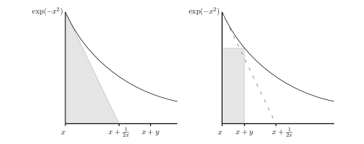
Figure 3. If $x+\frac{1}{2x}\leq x+y$, then we bound $\int_{x}^{x+y}\exp(-t^{2})dt$ from below by the area of a triangle. If $x+\frac{1}{2x}>x+y$, then we use the area of a rectangle to bound this integral from below.

Therefore, using the trivial bound $0$ for $\ell=n$ and $\ell=n-1$, we get

$$\mathbb{E}(Z_{b_{n}}\mid A_{I}) \geq\sum_{1\leq\ell\leq n-2:v_{\ell}=0,\epsilon a^{2}_{\ell}\leq 1/4}\frac{\sqrt{2}\epsilon a_{\ell}}{4\sqrt{\pi}(2^{\ell-n}+1/2)}\exp(-(\frac{2^{\ell-n}+1/2}{\sqrt{2\epsilon}a_{\ell}})^{2})$$ (19)

$$\ \ \ \ \ \ \ \ \ \ \ \ \ \ \ +\sum_{1\leq\ell\leq n-2:v_{\ell}=0,\epsilon a^{2}_{\ell}>1/4}\frac{1}{2\sqrt{2\pi}a_{\ell}}\exp(-(\frac{2^{\ell-n}+1}{\sqrt{2\epsilon}a_{\ell}})^{2})$$

$$\geq\sum_{1\leq\ell\leq\frac{5}{6}n:v_{\ell}=0,\epsilon a^{2}_{\ell}\leq 1/4}\frac{\sqrt{2}\epsilon a_{\ell}}{3\sqrt{\pi}}\exp(-(\frac{2^{\ell-n}+1/2}{\sqrt{2\epsilon}a_{\ell}})^{2})$$

$$\ \ \ \ \ \ \ \ \ \ \ \ \ \ \ +\sum_{1\leq\ell\leq n-2:v_{\ell}=0,\epsilon a^{2}_{\ell}>1/4}\frac{1}{2\sqrt{2\epsilon}a_{\ell}}\exp(-(\frac{5}{4\sqrt{2\pi}a_{\ell}})^{2}).$$

With (1) we see that

$$1\geq\mathbb{E}(Z_{b_{n}})\geq\sum_{I:balanced}\mathbb{E}(Z_{b_{n}}\mid A_{I})\mathbb{P}(A_{I}),$$ (20)

where the sum is over all intervals $I$ that are balanced. That means if we can bound $\mathbb{E}(Z_{b_{n}}\mid A_{I})$ from below by a number $C(n)$ only depending on $n$ (and not depending on the choice of the balanced interval $I$), then $\mathbb{P}(Y_{n}(I)\text{ for some balanced interval }I)$ is bounded from above by $1/C(n)$.

Now we will consider three cases, namely subsequences $(a_{n_{k}})$ of $(a_{n})$ with $a_{n_{k}}\to\infty$, $a_{n_{k}}\to 0$, and otherwise.

We start with the latter case. Here, call an interval $I$ balanced if the sequence $v_{1},\dots,v_{n}$ contains at least $n/3$ zeros and otherwise unbalanced. Then, we see that (19) goes to infinity.

To estimate the probability that $Y_{n}(I)$ happens for some unbalanced interval $I$ notice that the number of such intervals is bounded from above by $e^{-c_{5}n}2^{n}$ for some constant $c_{5}>0$. By (11) this gives

$$\mathbb{P}(Y_{n}(I)\text{ for some unbalanced interval }I)\leq\left\{\begin{array}[]{l l}e^{-c_{5}n},&\text{ if }a_{n}\leq 1,\\ e^{-c_{5}n}a_{n},&\text{ if }a_{n}>1.\end{array}\right.$$ (21)

But note for the case of $a_{n}>1$ that we note that $a_{n}\leq 2^{n/2}$. Thus, (21) goes to 0 for $n\rightarrow\infty$. It follows that $\inf_{n}\mathbb{P}(Y_{b_{n}}>0)=0$.

We proceed with the case that there is a subsequence $(a_{n_{k}})$ of $(a_{n})$ with $a_{n_{k}}\to 0$. We use the same definition of balanced intervals as in the case before. Assume there is a sequence $(c_{n})$ with $\sum_{n=1}^{\infty}c_{n}=\infty$ and fixed but arbitrary small $\delta>0$ and an $n_{0}>0$ such that for all $n\geq n_{0}$

$$\frac{1}{c_{n}}\geq a_{n}\geq\sqrt{\frac{1}{(8-\delta)\epsilon\ln{\frac{1}{c_{n}}}}}.$$

Now take the subsequence $(a_{n_{k}})$ such that for all $n_{k}\geq n_{0}$

$$\frac{1}{2\sqrt{\epsilon}}\geq a_{n_{k}}\geq\sqrt{\frac{1}{(8-\delta)\epsilon\ln{\frac{1}{c_{n_{k}}}}}}.$$

The right inequality is equivalent to

$$-\frac{1}{(8-\delta)\epsilon a_{n_{k}}^{2}}\geq\ln{c_{n_{k}}}.$$

From this it follows that

$$-\frac{1}{8\epsilon a_{n_{k}}^{2}}+\ln{a_{n_{k}}}\geq\ln{c_{n_{k}}},$$

and

$$\exp{(-\frac{1}{8\epsilon a_{n_{k}}^{2}})}\cdot{a_{n_{k}}}\geq{c_{n_{k}}}.$$

With (19) and the argument following (19) we have

$$\inf_{n}\mathbb{P}(Y_{n}(I)\text{ for some unbalanced interval }I)=0.$$

Thus together with (21) it follows $\inf_{n}\mathbb{P}(Y_{b_{n}}>0)=0$.

To finish we look at the case of having a subsequences $(a_{n_{k}})$ of $(a_{n})$ with $a_{n_{k}}\to\infty$. Let $d_{n}:=\frac{1}{2}\sum_{i=1}^{n}\frac{1}{a_{i}}$. Now we define an interval $I$ to balanced if the corresponding binary address $v_{1},\dots,v_{n}\in\{0,1\}^{n}$ fulfills that $\sum_{i=1}^{n}\frac{v_{i}}{a_{i}}\leq d_{n}$.

Observe that we can apply the exceptional Chebychev inequality, for a positive number $k$,

$$\mathbb{P}\big{(}\sum_{i=1}^{n}\frac{v_{i}}{a_{i}}\geq d_{n}\big{)} \leq\mathbb{E}\Big{(}\exp\big{[}k(\sum_{i=1}^{n}\frac{v_{i}}{a_{i}}-d_{n})\big{]}\Big{)}$$ (22)

$$=\exp(-kd_{n})\cdot\prod_{i=1}^{n}\mathbb{E}\big{(}\exp(k\frac{v_{i}}{a_{i}})\big{)}$$

$$=\exp(-kd_{n})\frac{1}{2}\big{(}1+\exp(\frac{k}{a_{i}})\big{)}.$$

Note that if $\sum_{i=1}^{n}\frac{1}{a_{i}}\leq C\log n$, then we can find a $k>0$ for (22) such that $\mathbb{P}\big{(}\sum_{i=1}^{n}\frac{v_{i}}{a_{i}}\geq d_{n}\big{)}\cdot a_{n}\to 0$. By (11) it follows that the probability that $Y_{n}(I)$ happens for some unbalanced interval goes to $0$, and also $\mathbb{P}(Y_{n}(I)\text{ for some balanced interval }I)$ goes to $0$ as $n\to\infty$ by (19) and the argument following (19).

The claim follows now from (8).

∎

If we require the sequence $(a_{n})$ to fulfill $a_{n}^{2}-\frac{1}{2}a_{n+1}^{2}\geq x_{n}$ for some positive sequence $(x_{n})$ with $x_{n}<a_{n}^{2}$ for all $n$ instead of the condition $a_{n}^{2}-\frac{1}{2}a_{n+1}^{2}\geq\epsilon a_{n}^{2}$ for all $n$ that we used so far, then the analogue to the Theorems 3.1 and 3.3 is the following result.

Corollary 3.5.

If the sequence $(a_{n})$ fulfills $a_{n}^{2}-\frac{1}{2}a_{n+1}^{2}\geq x_{n}$ for some positive sequence $(x_{n})$ with $x_{n}<a_{n}^{2}$ for all $n$, then $\mathbb{P}(\operatorname{\mathcal{Z}}(B-f_{b})\cap C_{b}\neq\emptyset)>0$ holds if either $\sum_{n=1}^{\infty}\frac{a^{2}_{n}}{\sqrt{x_{n}}}<\infty$, or $\sum_{n=1}^{\infty}\frac{1}{\sqrt{x_{n}}}<\infty$, and

$\mathbb{P}(\operatorname{\mathcal{Z}}(B-f_{b})\cap C_{b}\neq\emptyset)=0$ holds if

(i) there is a sequence $(c_{n})$ with $\sum_{n=1}^{\infty}c_{n}=\infty$ and a fixed but arbitrary small $\delta>0$ and an $n_{0}>0$ such that for all $n\geq n_{0}$

$$\frac{1}{c^{2}_{n}}\geq x_{n}\geq\frac{1}{(8-\delta)\ln{\frac{1}{c_{n}}}},$$

or if

(ii)$\sum_{\ell=1}^{n}\frac{1}{\sqrt{x_{\ell}}}\rightarrow\infty$ for $n\rightarrow\infty$ and if there is a constant $C>0$ such that $\sum_{\ell=1}^{n}\frac{1}{\sqrt{x_{\ell}}}\leq C\log n$ for all $n>0$.

Proof.

Analogously to the proofs of the Theorems 3.1 and 3.3. ∎

Theorems 3.1 and 3.3 do not give an answer for certain sequences $(a_{n})$, for instance $a_{n}=\frac{1}{n}$, whether or not the zero set of $B-f_{b}$ contains points of the corresponding generalized Cantor set with positive probability. It is natural to ask if we can strengthen the methods we used to get a stronger result.

Note that by (9) and (10) the probability of the event that Brownian motion hits a diagonal of a rectangle is up to a constant the maximum of the probabilities of the events that that Brownian motion hits the lower horizontal side or the right vertical side of the rectangle. Thus, it worth looking at the event that Brownian motion hits the lower horizontal side of the rectangle instead of the event $Z_{n}(J_{j})$ for the estimate (13). Call the former event $X_{n}(J_{j})$, then we get instead of (13)

$$\mathbb{P}(X_{n}(J_{j})\mid A_{I})\geq\int_{x}^{x+2^{-2n}a_{n}^{2}}\frac{1}{\sqrt{2\pi t}}\exp(-\frac{{(2^{-\ell-1}+2^{-n}j)}^{2}}{2t})dt$$

for some point $x\in[\sqrt{\epsilon}2^{-2\ell}a_{\ell}^{2},2^{-2\ell}a_{\ell}^{2})$. But here we see that summing over all $j$ and $\ell$ would not give an expression that goes to infinity for $n\rightarrow\infty$ for any possible sequence $(a_{n})$. Thus, looking at the event that that Brownian motion hits the lower horizontal side cannot provide an improvement of the result 3.3.

Comparing

$$\int_{(j+2^{n-\ell-1})\frac{2^{\ell-n}}{\sqrt{\epsilon}a_{\ell}}-\frac{2^{\ell-n}}{a_{\ell}}}^{(j+2^{n-\ell-1})\frac{2^{\ell-n}}{\sqrt{\epsilon}a_{\ell}}}\frac{1}{\sqrt{2\pi}}\exp(-\frac{1}{2}t^{2})dt\\ \leq\frac{2^{\ell-n}}{\sqrt{2\pi}a_{\ell}}\exp\Big{(}-\frac{1}{2}{((j+2^{n-\ell-1})\frac{2^{\ell-n}}{\sqrt{\epsilon}a_{\ell}}-\frac{2^{\ell-n}}{a_{\ell}})^{2}}\Big{)},$$

to the estimate (15), and

$$\sum_{1\leq j\leq 2^{n-\ell-1}} \frac{2^{\ell-n}}{\sqrt{2\pi}a_{\ell}}\exp\Big{(}-\frac{1}{2}{((j+2^{n-\ell-1})\frac{2^{\ell-n}}{\sqrt{\epsilon}a_{\ell}}-\frac{2^{\ell-n}}{a_{\ell}})^{2}}\Big{)}$$

$$\leq\int_{0}^{2^{n-\ell-1}}\frac{2^{\ell-n}}{\sqrt{2\pi}a_{\ell}}\exp\Big{(}-\frac{1}{2}{((j+2^{n-\ell-1})\frac{2^{\ell-n}}{\sqrt{\epsilon}a_{\ell}}-\frac{2^{\ell-n}}{a_{\ell}})^{2}}\Big{)}dj$$

$$=\sqrt{\frac{\epsilon}{\pi}}\int_{\frac{\frac{1}{2}-\sqrt{\epsilon}2^{\ell-n}}{\sqrt{2\epsilon}a_{\ell}}}^{\frac{1-\sqrt{\epsilon}2^{\ell-n}}{\sqrt{2\epsilon}a_{\ell}}}\exp(-t^{2})dt$$

$$\leq\frac{1}{2\sqrt{2\epsilon}a_{\ell}}\exp(-(\frac{\frac{1}{2}-\sqrt{\epsilon}2^{\ell-n}}{\sqrt{2\epsilon}a_{\ell}})^{2}),$$

to (16) and (19) we see that for the inequality (7) we cannot improve the result 3.3 by using better bounds.

For the proof of Theorem 3.1 it is easy to check that better estimates can not provide a stronger result. In particular, by bounding $S(z)$ from above we see that the second moment can at most be improved by a constant factor.

Remark 3.6.

Theorems 3.1 and 3.3 can be extended to more classes of Cantor-like functions. We consider for a given positive, real sequence $(a_{n})$ a sequence $(b_{k,n})$ defined by $b_{k,n}:=(k^{-n}\cdot a_{n})^{2}$ with $k>0$. For this sequence we define a corresponding $k$-Cantor-type set and denote it by $C_{b_{k}}$. Take a closed interval $I$ of length $b_{k,0}$. Define $\mathfrak{C}_{b_{k,1}}$ as the set consisting of $k$ disjoint closed subintervals of $I$ of length $b_{k,1}$, the left one (for which the left endpoint coincides with the left endpoint of $I$), the right one (for which the right endpoint coincides with the right endpoint of $I$) and $k-2$ intervals such that two neighboring intervals have the distance $\frac{b_{k,0}-kb_{k,1}}{k-1}$. Continue recursively, if $J\in\mathfrak{C}_{b_{n}}$, then include in the set $\mathfrak{C}_{b_{n+1}}$ its $k$ closed subintervals of length $b_{k,n+1}$. Define the set $C_{b_{n}}$ as the union of all the intervals from $\mathfrak{C}_{b_{n}}$. For any $n$, the family $\mathfrak{C}_{b_{k,n}}$ is the set of all connected components of the set $C_{b_{k,n}}$. The $k$-Cantor set is a compact set defined as $C_{b_{k}}=\bigcap_{n=1}^{\infty}C_{b_{k,n}}$. Now we construct a $k$-Cantor-type function corresponding to the $k$-Cantor type set above. Define the function $f_{b_{k,1}}$ so that it has values $0$ and $1$ at the left and the right endpoint of the interval $I$, respectively, values $1/k$ on the most left, $2/k$ on the second most left, …, and $(k-1)/k$ on the least most left of the $k-1$ disjoint intervals of the set $I\backslash{C}_{b_{k,1}}$, and interpolate linearly on the intervals in $\mathfrak{C}_{b_{k,1}}$. Recursively, construct the function $f_{b_{k,n+1}}$ so that for every interval $J=[s,t]\in\mathfrak{C}_{b_{k,n}}$, the function $f_{b_{k,n+1}}$ agrees with $f_{b_{k,n}}$ at $s$ and $t$, it has values $(f_{b_{k,n}}(t)-f_{b_{k},n}(s))\cdot\frac{1}{k}+f_{b_{k},n}(s)$ on the most left, $(f_{b_{k,n}}(t)-f_{b_{k},n}(s))\cdot\frac{2}{k}+f_{b_{k},n}(s)$ on the second most left, …, and $(f_{b_{k,n}}(t)-f_{b_{k},n}(s))\cdot\frac{k-1}{k}+f_{b_{k},n}(s)$ on the least most left of the $k-1$ disjoint intervals of the set $J\backslash C_{b_{k,n+1}}$ and interpolate linearly on the intervals in $\mathfrak{C}_{b_{k,n+1}}$. See Figure 4 for an example of $k=3$.

Figure 4. First three approximations of the $3$-Cantor type function on the interval $[1,2]$ (functions $f_{b_{3,n}}$ from the construction for $b_{1}=0.2$, $b_{2}=0.04$ and $b_{3}=0.01$, or $a_{1}=\sqrt{1.8}$, $a_{2}=1.8$ and $a_{3}=2.7$, respectively. Approximations of the Cantor set $C_{b_{3}}$ are drawn in bold).

As in section 2, for a fixed $k>1$ we fix an arbitrary small $\epsilon>0$ and require the sequence $(a_{n})$ to fulfill the condition $a_{n}^{2}-\frac{1}{k}a_{n+1}^{2}\geq\epsilon a_{n}^{2}$ (or equivalently $b_{k,n}-kb_{k,n+1}\geq\epsilon b_{k,n}$) for all $n$. Then, Theorems 3.1 and 3.3 hold also for the $k$-Cantor-type function.

Further, note that if we have the weaker condition $b_{k,n}-kb_{k,n+1}>0$ for all $n$, then we can apply Corollary 3.5.

4. Isolated zeros - general criteria

We will now state two criteria determining whether a zero of $B-f$ for a continuous function $f$ is almost surely isolated or not isolated. For any function $g$ defined on some subset (or the whole) of $\mathbb{R}^{+}$ denote by $\operatorname{\mathcal{Z}}(g)$ the set of zeros of $g$ in $(0,\infty)$. Recall that we denoted the middle $\alpha$-Cantor function by $f_{\alpha}$. Antunović, Burdzy, Peres, and Ruscher showed that for every $\alpha<1/2$ there is an $\alpha$-Hölder continuous function $f\colon\mathbb{R}^{+}\to\mathbb{R}$ such that the set $\operatorname{\mathcal{Z}}(B-f)$ has isolated points with positive probability, see Theorem 1.2 of [ABPR]. To show this result they proved that the zero set of $B-f_{\alpha}$ has isolated points with positive probability for $\alpha>1/2$. We want to extend that result for our generalized class of Cantor functions in the next section. First we need to look at a criterion for having isolated zeros.

Proposition 4.1.

Let $f\colon\mathbb{R}^{+}\to\mathbb{R}$ be a continuous function.

• Let $A$ be a closed subset of $\mathbb{R}^{+}$ such that for any $t\in A$

  $$\liminf_{s\to t}\frac{|f(s)-f(t)|}{\sqrt{2|t-s|\log\log{\frac{1}{|t-s|}}}}>1.$$

  Then, almost surely any point in $\operatorname{\mathcal{Z}}(B-f)\cap A$ is isolated in $\operatorname{\mathcal{Z}}(B-f)$.

• Let $A\subset\mathbb{R}^{+}$ be a set such that for any $t\in A$

  $$\limsup_{s\to t}\frac{|f(s)-f(t)|}{\sqrt{2|t-s|\log\log{\frac{1}{|t-s|}}}}<1.$$

  Then, almost surely any point in $\operatorname{\mathcal{Z}}(B-f)\cap A$ is not isolated in $\operatorname{\mathcal{Z}}(B-f)$.

Proof.

(i) We define a sequence of stopping times $(\tau_{n})$. Let

$$\tau_{0}=\min\left\{t\in A:B(t)=f(t)\right\},$$

and

$$\tau_{n}=\min\left\{t\in A,t>\tau_{n-1}:B(t)=f(t)\right\}.$$

Since $\tau_{n}$ is a stopping time for every $n$, $t\mapsto B(\tau_{n}+t)-B(\tau_{n})$ is a Brownian motion if $\tau_{n}<\infty$. We can apply the law of iterated logarithm (see Theorem 5.1 in [MP]) to get that almost surely for all $n$ we have

$$\liminf_{t\downarrow 0}\frac{B(\tau_{n}+t)-B(\tau_{n})}{\sqrt{2t\log\log{\frac{1}{t}}}}=-1\ \text{ and }\limsup_{t\downarrow 0}\frac{B(\tau_{n}+t)-B(\tau_{n})}{\sqrt{2t\log\log{\frac{1}{t}}}}=1.$$

Thus all $\tau_{n}$’s are isolated from the right. By the reverse property of Brownian motion all $\tau_{n}$’s are also isolated from the left. This implies that $\tau_{n}$ converges to $\infty$ since A is a closed set. Therefore, every zero in $A$ is contained in the sequence $(\tau_{n})$.

(ii) Assume that there exists a an isolated zero in the set $A$ with positive probability. Then, there is a $q\in\mathbb{Q}$ such that $\tau_{q}=\min\left\{t\geq q:B(t)=f(t)\right\}$ is an isolated zero in $A$.

Since $\tau_{q}$ is a stopping time, the process $B_{q}(t)=B(\tau_{q}+t)-B(\tau_{q})$, is, by the strong Markov property, a Brownian motion independent of the sigma algebra $\mathcal{F}_{\tau_{q}}$. By the law of the iterated logarithm it follows that $\tau_{q}$ is not isolated.

∎

Note that (i) is a stronger statement than Proposition 2.2.(i) of [ABPR] for closed subsets of $\mathbb{R}^{+}$. According to Proposition 2.2.(ii) of [ABPR] almost surely all isolated points of $\operatorname{\mathcal{Z}}(B-f)$ are located inside the set $A_{f}^{+}\cup A_{f}^{-}$, where

$A_{f}^{+}=\{t\in\mathbb{R}^{+}:\lim_{h\downarrow 0}\frac{f(t+h)-f(t)}{\sqrt{h}}=\infty\}$ and

$A_{f}^{-}=\{t\in\mathbb{R}^{+}:\lim_{h\downarrow 0}\frac{f(t+h)-f(t)}{\sqrt{h}}=-\infty\}$. In particular, (ii) shows that not all points in $\{A_{f}^{+}\cup A_{f}^{-}\}\cap\operatorname{\mathcal{Z}}(B-f)$ have to be isolated in $\operatorname{\mathcal{Z}}(B-f)$.

5. Isolated zeros of Brownian Motion minus Cantor function

In [ABPR] it was shown for the middle $\alpha$-Cantor function $f_{\alpha}$ that $B-f_{\alpha}$ has isolated zeros with positive probability if $\alpha>1/2$. Recall that for $a_{n}=\frac{1}{x^{n}}$ with some $x>1$ gives $b_{n}:=(2^{-n}\cdot\frac{1}{x^{n}})^{2}=(2x)^{-2n}$ which corresponds to $\alpha=1-\frac{1}{x}$. Therefore, the following proposition extends this result of [ABPR].

Proposition 5.1.

The set $\operatorname{\mathcal{Z}}(B-f_{b})$ has isolated points with positive probability if $\sum_{n=1}^{\infty}a_{n}<\infty$, and no isolated points almost surely if $\sum_{n=1}^{\infty}\frac{1}{a_{n}}<\infty$.

Proof.

First we will prove that if $\sum_{n=1}^{\infty}a_{n}<\infty$, then $\operatorname{\mathcal{Z}}(B-f_{b})$ has isolated points with positive probability. For $A\subset\mathbb{R}^{+}$ define $Z(A)$ as the event $\{\operatorname{\mathcal{Z}}(B-f_{b})\cap A\neq\emptyset\}$. We claim that there exists a constant $c_{1}$, such that for any interval $J\subset[0,1]$ of length $|J|$, we have

$$\mathbb{P}(Z(C_{b}\cap f_{b}^{-1}(J)))\leq c_{1}|J|.$$ (23)

In order to show this statement, fix an interval $J$ and take the biggest integer $n$ satisfying $|J|\leq 2^{-n}$. Notice that $J$ can be covered by two consecutive binary intervals $J_{1}$ and $J_{2}$ of length $2^{-n}$. Moreover, there are consecutive $I_{1},I_{2}\in\mathfrak{C}_{b_{n}}$ such that $f_{b}(I_{i})=J_{i}$ for $i=1,2$, and $C_{b}\cap f_{b}^{-1}(J)\subset I_{1}\cup I_{2}$.

Now we will again use the notation that we introduced in the proof of Theorem 3.1. Assume that $\operatorname{\mathcal{Z}}(B-f_{b})\cap C_{b}\neq\emptyset$ and denote the first zero of $B(t)-f_{b}(t)$ in the generalized Cantor set $C_{b}$ by $\tau$ ($\tau$ exists since $\operatorname{\mathcal{Z}}(B-f_{b})\cap C_{b}$ is a closed set). For an interval $I=[s,t]\in\mathfrak{C}_{b_{n}}$ assume that $\tau\in I$. Since $\tau$ is a stopping time, and by Brownian scaling, the conditional probability $\mathbb{P}\Big{(}Z_{n}(I)\mid\mathcal{F}_{\tau},\tau\in I\Big{)}$ is equal to the probability that Brownian motion at time $1$ is between $y_{1}=(f_{b}(s)-f_{b}(\tau))(t-\tau)^{-1/2}$ and $y_{2}=(f_{b}(t)-f_{b}(\tau))(t-\tau)^{-1/2}$. Since $f_{b}(s)\leq f_{b}(\tau)\leq f_{b}(t)$ we see that $y_{1}\leq 0$ and $y_{2}\geq 0$. Moreover, $t-\tau\leq 4^{-n}=(f_{b}(t)-f_{b}(s))^{2}$ leads to $y_{2}-y_{1}\geq 1$.

Thus we can bound the probability

$$\mathbb{P}\Big{(}Z_{n}(I)\mid\mathcal{F}_{\tau},\tau\in I\Big{)}\geq\mathbb{P}(0\leq B(1)\leq 1)=\alpha,$$ (24)

for some $\alpha>0$. Hence,

$${\alpha}\mathbb{P}(Z(C_{b}\cap I_{i}))\leq\mathbb{P}(Z_{n}(I_{i})).$$ (25)

But by the first inequality in (1), the probability on the right hand side of (25) is bounded from above by $2^{-n}$. Applying this fact in (25) and summing the expression for $i=1,2$, we obtain (23).

By Theorem 3.1 the set $\operatorname{\mathcal{Z}}(B-f_{b})\cap C_{b}$ is non-empty with some probability $p>0$. For every $n>0$ take an arbitrary $b^{\prime}_{n}=(2^{-n}a^{\prime}_{n})^{2}$ such that $b_{n}<b^{\prime}_{n}<2^{-2n}$ and $n_{0}$ such that $\sum_{n\geq n_{0}}a^{\prime}_{n}\leq p/(2c_{1})$.

For $n\geq n_{0}$ consider the interval $J_{k,n}=[k2^{-n}-\frac{1}{2}\sqrt{b^{\prime}_{n}},k2^{-n}+\frac{1}{2}\sqrt{b^{\prime}_{n}}]$ and define the set $M_{n_{0}}=\bigcup_{n\geq n_{0}}\bigcup_{0\leq k\leq 2^{n}}J_{k,n}$. By (23) and the choice of $n_{0}$, we see that $\mathbb{P}(Z(C_{b}\cap f_{b}^{-1}(M_{n_{0}})))\leq p/2$. Hence, the event that there is a zero of $B(t)-f_{b}(t)$ in the set $C_{b}\cap\text{Int}(C_{b_{n_{0}}})\backslash f_{b}^{-1}(M_{n_{0}})$ has probability of at least $p/2$ (here $\text{Int}(C_{b_{n_{0}}})$ is the interior of the set $C_{b_{n_{0}}}$). Now the claim follows if we prove that any such zero is isolated. Take $t\in C_{b}\cap\text{Int}(C_{b_{n_{0}}})\backslash f_{b}^{-1}(M_{n_{0}})$ and any $s\neq t$ in the same connected component of $\text{Int}(C_{b_{n_{0}}})$. The biggest integer $\ell$ such that both $s$ and $t$ are contained in the same interval of $\mathfrak{C}_{b_{\ell}}$ satisfies $\ell\geq n_{0}$. Further, $|f_{b}(s)-f_{b}(t)|\geq\frac{1}{2}\sqrt{b^{\prime}_{\ell}}$ and $b_{\ell+1}\leq|s-t|\leq b_{\ell}$. With Proposition 4.1(i) the claim follows by taking for example $a^{\prime}_{n}=\sqrt{a_{n}}$ for $n$ big enough.

For the second part of the claim we just need to apply the Proposition 2.2.(i) of [ABPR] (see above). ∎

References

- [ABPR] T. Antunović, K. Burdzy, Y. Peres, and J. Ruscher. Isolated zeros for Brownian motion with variable drift. Electronic Journal of Probability. Vol. 16, No. 65: 1793–1814, 2011.
- [APV] T. Antunović, Y. Peres, and B. Vermesi. Brownian motion with variable drift can be space-filling. Proc. Amer. Math. Soc. Vol. 139: 3359-3373, 2011.
- [HT] G. G. Hamedani, M. N. Tata, On the determination of the bivariate normal distribution from distributions of linear combinations of the variables. The American Mathematical Monthly. Vol. 82, No. 9: 913–915, 1975.
- [MP] P. Mörters and Y. Peres. Brownian Motion. Cambridge Series in Statistical and Probabilistic Mathematics. Cambridge University Press, 2010.
- [PS] Y. Peres and P. Sousi. Brownian motion with variable drift: 0-1 laws, hitting probabilities and Hausdorff dimension. Available at http://arxiv.org/abs/1010.2987v1.
- [R12] J. Ruscher. A note on fast times of Brownian motion with variable drift. Preprint, 2012.
- [RY] Daniel Revuz and Marc Yor. Continuous martingales and Brownian motion, volume 293 of Grundlehren der Mathematischen Wissenschaften [Fundamental Principles of Mathematical Sciences]. Springer-Verlag, Berlin, third edition, 1999.
- [TW] S. J. Taylor and N. A. Watson. A Hausdorff measure classification of polar sets for the heat equation. Math. Proc. Cambridge Philos. Soc., Vol. 97, No. 2: 325–344, 1985.