Phase extraction in disordered isospectral shapes

Abstract

The phase of the electronic wave function is not directly measurable but, quite remarkably, it becomes accessible in pairs of isospectral shapes, as recently proposed in the experiment of Christopher R. Moon et al., Science 319, 782 (2008). The method is based on a special property, called transplantation, which relates the eigenfunctions of the isospectral pairs, and allows to extract the phase distributions, if the amplitude distributions are known. We numerically simulate such a phase extraction procedure in the presence of disorder, which is introduced both as Anderson disorder and as roughness at edges. With disorder, the transplantation can no longer lead to a perfect fit of the wave functions, however we show that a phase can still be extracted - defined as the phase that minimizes the misfit. Interestingly, this extracted phase coincides with (or differs negligibly from) the phase of the disorder-free system, up to a certain disorder amplitude, and a misfit of the wave functions as high as $\sim 5\%$, proving a robustness of the phase extraction method against disorder. However, if the disorder is increased further, the extracted phase shows a puzzle structure, no longer correlated with the phase of the disorder-free system. A discrete model is used, which is the natural approach for disorder analysis. We provide a proof that discretization preserves isospectrality and the transplantation can be adapted to the discrete systems.

I Introduction

Famous mathematical problems sometimes attracted a great interest from physicists as well. One such problem was the isospectrality debate launched by Kac in 1966 Kac when he asked: ”Can one hear the shape of a drum”? It was known that the spectrum uniquely determined the area and the perimeter of a ”drum”, but whether it also contained the full shape information was yet to be researched. It wasn’t until 1992 that Gordon et.al. Gordon , in a milestone paper, answered negatively to the famous question by finding different (noncongruent) shapes with identical spectra. However, isospectrality remains a high exception, only 17 such classes of pairs being known RMP , and it is believed that no others exist. Soon after the paper by Gordon et al.Gordon , Wu et al. Wu and Driscoll Driscoll found explicitly the first eigenvalues and eigenfunctions of two - the most simple and most famous - such isospectral shapes, called ”Bilby” and ”Hawk” (see Fig.1). There has been also immediate experimental interest of realizing such isospectral domains, by Sridar and Kudrolli Sridar , in a microwave cavities experiment. Other boundary conditions for the isospectral shapes have also been discussed in Driscoll2 ; Dowker ; Levitin . Mathematical and physical aspects of isospectrality have been reviewed by Giraud and Thas RMP - including also pioneering contributions of the authors.

Recently - and this was the motivation of our paper - isospectrality has found a direct application in experimental quantum mechanics, by allowing the extraction of the electron’s phase, in a non-interferometric way. We refer to the experiment of Moon et al. Science , who realized isospectral shapes by planting CO molecules on copper surface with the use of an STM tip. The principle of the phase extraction is simple: it can be shown that, if one has two isospectral shapes, one can build the eigenfunctions of one shape by using combination of parts from the corresponding eigenfunction of the other shape. The procedure is called ”transplantation” (see Appendix A) and this brings supplementary information which are used to find the phase distribution of the eigenfunctions.

Prior to the experiment of Moon et al. Science , the phase measurement -in mesoscopic physics- has already attracted a great interest. Naturally, the first experiments used interference geometries, namely Aharonov-Bohm interferometers with embedded quantum dots. Such experiments (e.g. Schuster ) aimed to extract the phase of the electron transmittance through a quantum dot and they generated a number of intriguing questions, that are still open. We mention briefly the universal phase lapse between resonances (called by some authors ”the longest standing puzzle in mesoscopic physics” - e.g. Oreg ; Karr ) for a many-electron dot, or the reduced variation of the phase (with fractions of $\pi$ on some resonances and between them) for a few-electrons quantum dot Avinun . As was easy to expect, these open questions attracted many theoretical attempts to explain them (see for instance the recent papers Oreg ; Karr ; Goldstein ; TNA ; Rontani ; Puller ; Buchholz ; Racec and references therein). The two existing phase measurement setups (by interferometry or by use of isospectral shapes), although different, present similarities comment1 .

In this paper, we focus on the study of isospectral shapes (in particular the Bilby-Hawk pair) under the influence of disorder, with an emphasis on the phase extraction procedure. The aspect should be of interest because the experimental conditions, for instance, are never quite perfect, and isospectrality can only be closely approached. If, for instance, the isospectral shapes are carefully prepared on a flat surface, the disorder effects may come from small defects, oscillations of the atoms due to temperature, tiny movements of the STM measurement tip, etc. The are many ways in which disorder or impurities can be introduced. In this paper we present the result of averaging (the measurable quantities, such as energy levels and wave functions amplitudes) over large ensembles of disorder configurations of variable amplitude (diagonal Anderson disorder is considered). With disorder, isospectrality, as well as the transplantation procedure do not hold rigourously. One can however still define a ”measurable” or ”extracted” phase simulating the experimental procedure: we will use the (disordered averaged) wave function amplitudes and search numerically the phase distribution that leads to the best fit after transplantation. It will be found that this extracted phase coincides - up to negligible differences - with the phase of the ”clean” shapes, if the disorder is below a given amplitude.

We consider also the effect of edge roughness, with similar conclusions, namely that a certain degree of roughness can be allowed. Therefore the ”perfect” conditions are not necessary for a correct phase extraction. A discrete model is used, as being the most suitable approach for disorder analysis. The discrete approach allows easy tailoring of any shapes, which remain isospectral if their continuous counterparts are isospectral (see the proof in Appendix A). Another justification for choosing a discrete model comes again from the phase measurement experiment of Moon et. al Science , where the wave functions amplitudes (used for transplantation) were measured in a finite number of points on the surface.

The outline of the paper is as follows: in Section II we introduce our discrete model, Section III contains the main results, which are summarized in Section IV. Appendix A gives a proof that isospectrality holds in the discrete representation and Appendix B offers a comparison between continuous and discrete models.

II The discrete model

We choose a discrete approach meaning that the isospectral shapes will be described by a number of sites (noted with i or j) that belong to a rectangular lattice with given on-site energies $\epsilon_{i}$ and hopping integrals $t_{i,j}$. A generic Hamiltonian can be written as:

$$H=\sum_{i}\epsilon_{i}|i\rangle\langle i|+\sum_{i,j}t_{i,j}|i\rangle\langle j|.$$ (1)

$t_{i,j}$ is chosen to be equal with 1 (or energy unit) for the nearest neighbor sites and $0$ otherwise and the diagonal energies $\epsilon_{i}$ are equal to 0 for disorder free shapes or are given random values in the interval $[-W/2,W/2]$ in the presence of Anderson disorder with amplitude W.

The particular shapes described by the Hamiltonian in Eq.1 are determined by the way in which the sites are inter-connected, two examples being the isospectral Bilby and Hawk drums shown in Fig.1. The total number of sites inside each shape can be calculated if we give the value $N$ which is the number of sites on the hypotenuse of an elementary triangle (for Fig.1, $N=7$) sites .

Figure 1: (Color online) The isospectral shapes ”Bilby” and ”Hawk”. They are represented by a discrete set of points at the intersections of the thin dashed lines. Each shape is divided in 7 triangles, for the purpose of transplantation (see description in text). The triangles are noted with $\alpha$=A,…,G for Bilby and $n$=1,…,7 for Hawk. One can see that some points are in the interior of triangles and others on the borders between triangles (thin red lines) or on the exterior borders (black continuous lines). The points on the exterior borders are considered to have infinite potential so the wave functions vanish on these points.

It is known that the continuous Bilby and Hawk shapes are isospectral. A natural question is whether the discrete Bilby and Hawk are also isospectral, for any discretization (i.e. any $N$), or is the continuous limit necessary in order to achieve this property? We prove that the first affirmation is correct and the isospectrality holds for any discretization. The proof is presented in Appendix A and is based on the transplantation method, similar to the continuous case. A further comparison between discrete and continuous models is discussed in Appendix B.

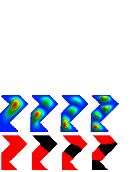
Figure 2: (Color online) The first four eigenmodes of Bilby: amplitudes (first row) and phases (second row). The black and red (gray) zones have opposite phases (the real wave function have opposite signs).

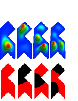
Figure 3: (Color online) The same as in Fig.2, for the first four Hawk modes.

We plot below the amplitudes and phases of the first four eigenmodes of Bilby (Fig.2) and Hawk (Fig.3), corresponding to a discretization with $N=21$. The plots are given for completeness. While the amplitudes plots can be found in literature for a large number of eigenmodes RMP , we found phase plots only in the experimental paper Science . A discussion is necessary regarding the plotted phase. The shapes we discuss are closed systems and their eigenfunctions are considered real. Therefore the phase can only be $0$ or $\pi$ corresponding to the sign $+$ or $-$ of the wave function on a particular site (see also the discussion in Science ). Obviously, the phase of a wave function is defined up to a constant, so what is relevant is the relative phase difference between the points on the surface. One can say that the fundamental mode on both Bilby and Hawk has the same phase on the entire surface (and we shall consider by convention that the wave function is positive, or has a ”$0$” phase, plotted red in Figs.2 and 3). The $2^{nd}$ mode has two regions of opposite phases and the third has two regions in-phase separated by a region of opposite phase, etc. The second and third modes have equal number of nodal lines for Bilby and Hawk, one nodal line for the second mode and two nodal lines for the third. Interestingly, the Bilby’s forth mode has three nodal lines, while Hawk’s forth mode has only two nodal lines, as isospectrality does not necessarily imply an equal number of nodal lines Gnutzmann . The two shapes are isospectral both in the continuous and in the discrete representations, and eigenfunctions of each shape can be built from the eigenfunctions of the other by the transplantation procedure (Appendix A). In particular, this allows the extraction of the phase distribution of the eigenfunctions Science . In the next section, it will be shown that a correct phase extraction is possible also in the presence of disorder (up to a certain disorder amplitude).

III Disorder effects and robustness of the phase extraction.

In this section we describe the phase extraction in the presence of disorder for our isospectral shapes. One can argue what is more relevant: to consider one single disorder configuration or the average (of the observables) over a number of disorder configurations. While both choices have their relevance, we prefer the second alternative in this paper. Even in the case of single electron transistors, for instance (or others transport phenomena where one electron at a time is involved), a steady value of the current can be read after thousands or more such single electron events. Temperature effects or tiny movements of the measurement tip (as in the STM case) can make each of these electrons to see a slightly different potential picture. Therefore averaging over a large number of disorder configurations corresponds to some realistic experimental conditions. Our plotted results refer to such averaging over a large number of disorder configurations (1000 for Figs. 6-8). There is also another reason for our choice to present the results for disorder averaging rather than individual disorder configurations. The averaging leads to convergent results, that can be easily reproduced. In fact, results regarding a single disorder configuration lead to the same main conclusions and they will be discussed briefly.

Figure 4: The Bilby-Hawk eigenvalue spectra (the first 10 eigenvalues) averaged over 1000 disorder configurations versus increasing disorder amplitude W. Notice that the spectra shift from their disorder-free values, but the two spectra remain identical to each other (in the limit of numerical errors).

Before going to the phase extraction problem -the main focus of our paper- we present briefly the effect of disorder averaging on the eigenvalue spectra of Bilby and Hawk in Fig. 4. When the Bilby-Hawk spectra are averaged over a large ensemble of disorder configurations, an expected energy shift is noticed when the disorder amplitude is increased. The initial spectra are roughly in the interval [-4:4] according to the theory for tight-binding model with nearest-neighbors hopping. For the disorder amplitude W=4 the spectra expands in the interval roughly $[-4.5:4.5]$ and also the level spacing presents a monotonic decrease from the bottom of the spectrum towards the middle (see also NAZ and references therein).

It is a known result that the tight-binding spectrum is expanding with increasing Anderson disorder (see, e.g. NAZ and references therein). In particular, this means than the lower eigenvalues move downwards. However, it is important to mention that the downward evolution of the lower eigenvalues is not just a mathematical aspect, but should also correspond to the physical situation: if a surface is affected by random positive and negative disorder potentials, the lowest eigenfunctions will tend to supplementary localize around the areas with low potentials, decreasing the eigenenergies. The effect is not significant for low disorder amplitudes, that are of interest for the phase extraction. What is interesting however, is that the Bilby and Hawk spectra remain very close to each other for any disorder amplitude, as seen in Fig.4 (the spectral lines for the two shapes practically coincide). The differences are one order of magnitude smaller than the standard deviation of the levels statistics. In other words, the isospectrality is robust against disorder averaging.

The next question, and -as mentioned- the main interest of our paper, is weather the measured (or ”extracted”) phase is also robust against disorder.

To begin with, the wave function square modules were averaged over a large number of disorder configuration, and we obtained $\langle|f_{Bi}(i)|^{2}\rangle$ and $\langle|f_{Ha}(i)|^{2}\rangle$ for Bilby and Hawk. We stress that in the experimental setup the localization probability is measured, this being the reason we mediate the square modules. In connection with experimental procedure Science one defines the ”extracted” or ”measurable” phase in the following way: it is the phase distribution that leads to the minimum misfit of the wave functions after transplantation, as described in the following numerical algorithm.

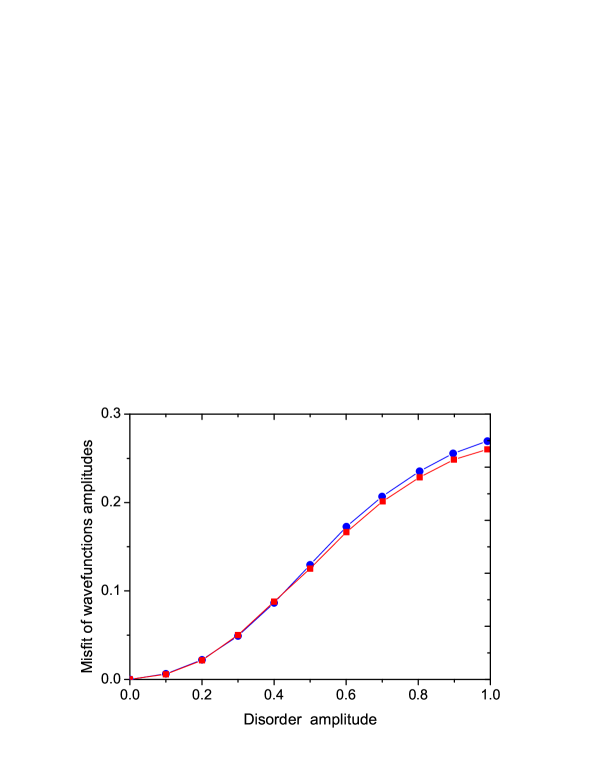
Figure 5: (Color online) The misfit between the calculated and the ”transplantated” eigenfunctions (see description in text) of Hawk shape, plotted versus the disorder amplitude W. The red line with square symbols corresponds to the first eigenvalue, the blue line (with circle symbols) corresponds to the second eigenvalue.

We start by assuming the disorder-free phase distribution for Bilby wave function (the one plotted in Fig.2). Assuming such initial phase distribution and the amplitude obtained as the squared of the disorder average function $\sqrt{\langle|f_{Bi}|^{2}\rangle}$ we have now a complete information about the Bilby wave function and this is used for transplantation (for transplantation one needs a full wave function information, both module and phase). The transplantation procedure produces a Hawk wave function $f_{Ha}^{T}$ following the recipe given by the Eqs. A5 and A6 in Appendix A. The square modulus of the transplantated wave function $|f_{Ha}^{T}(i)|^{2}$ is compared with the disorder average Hawk wave function $\langle|f_{Ha}(i)|^{2}\rangle$ and we define the misfit as the differences between the functions square modules in all sites versus the sum of the square modules:

$$Misfit=\frac{\sum_{i}Abs[\langle|f_{Ha}(i)|^{2}\rangle-|f_{Ha}^{T}(i)|^{2}]}{\sum_{i}\big{(}\langle|f_{Ha}(i)|^{2}\rangle+|f_{Ha}^{T}(i)|^{2}\big{)}}=\frac{\sum_{i}Abs[\langle|f_{Ha}(i)|^{2}\rangle-|f_{Ha}^{T}(i)|^{2}]}{2}.$$ (2)

In the absence of disorder, the misfit should be zero, and the phase distribution is the one for the unperturbed mode. In the presence of disorder, the misfit is finite and we have to search for the phase distribution of the initial Bilby function that minimize the misfit, repeating the above numerical algorithm. The convergent solution is the ’extracted’ or measured phase which is obtained when any change of a site phase would lead to a higher misfit.

The key question is whether this phase coincides with the ”unperturbed” phase (which is in fact desired to be measured) or is it a different phase distribution. The phases that minimize the misfit are determined for different disorder amplitudes W and are plotted in Figs. 6 and 7 for the first two modes of Bilby. The corresponding misfit (that was minimized by these phases) is plotted in Fig.5.

Figure 6: (Color online) Evolution with increasing disorder of the averaged -over $1000$ disorder configurations- wave function amplitude (first row) and the corresponding ”extracted phase” (second row) for the first mode of Bilby. The disorder amplitude, from left to right, is 0, 0.2, 0.3, 0.4 and 0.7. A significant deviation of the phase from the ideal (disorder-free) case can be noticed for disorder higher than $0.3$.

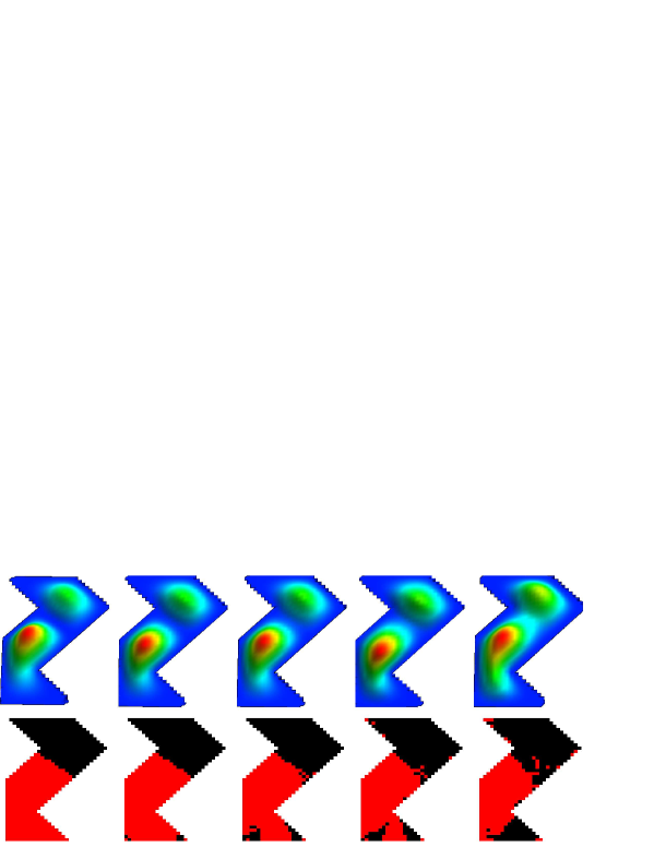
Figure 7: (Color online) The same as in Fig.6 for the second mode of Bilby.

It would be encouraging if even in the presence of the disorder, the best fit were still realized by the ”ideal” phase distribution (the one of the disorder-free system). This would make its extraction robust. Here is precisely the point we want to make in this paper. For low disorder it can be seen that indeed the ”ideal” phase actually ensures the best fit even if the wave function amplitudes are slightly changed and a finite misfit appears. Figures 6 and 7 suggest that a disorder higher than $0.2-0.3$ is needed for a significant variation of the extracted phase from the disorder-free configuration. The value $0.3$ corresponds to a misfit of the wave functions of about $5\%$. When the disorder is increased further, small zones of opposite phase appear inside the ”in-phase” zones (of the unperturbed case) and the nodal lines shifts. Such an ”extracted” phase is no longer related to the physical phase distribution of the unperturbed mode.

From Figs. 6 and 7 one can also see that the result of disorder averaging on the amplitudes of the wave functions is to extend the zones of high amplitude.

In the captions of Figs. 6 and 7, the disorder amplitude is expressed in terms of the hopping parameter between nearest-neighbors, which is taken by convention to be the energy unit (the usual approach in tight-binding models). However, the misfit of the wave functions after transplantation, plotted in Fig.5, is a directly measurable quantity. Therefore Figs. 6, 7 and 5 must be combined to give the conclusions in terms of the wave functions misfit. If the result is expressed in terms of wave functions misfit, it becomes independent of the energy scale convention and also independent of the discretization parameter N.

Our numerical results suggest that the ”extracted phase” differs negligibly from the ”ideal” phase if the misfit of the wave functions after transplantation is lower than a few percents (approx. $4-5\%$, as shown in this section).

We have checked also a large number of single disorder configurations (and not averages) and one can say that the general conclusion is the same: the extracted phase differs significantly from the ideal case when the misfit of the waves functions (after transplantation) exceeds $5\%$. In the case of single disorder configurations one can also talk about the ”intrinsic” phase of a certain eigenmode of the disordered Bilby (for instance). It is interesting to say that, with increasing disorder, the intrinsic phase will have shifted nodal lines, while the extracted phase tends to form new nodal lines separating small areas of opposite phases, resulting in a puzzle structure as seen for high disorders in Figs. 6 and 7.

To better connect our numerical simulation with experimental conditions, let us estimate, for instance (from Fig.4), that a disorder which shifts the energy levels with $10\%$ from the value of the (average) level spacing will significantly affect the phase extraction. A 2D quantum dot with area of $100nm^{2}$ may typically have a level spacing of $10meV$. Now if we assume that the thermal oscillations of atoms on the surface can be a source of disorder, we can say that a shift of the energy levels with $10\%$ from the level spacing could be expected for $K_{b}T=1meV$, resulting approximately $T=11K$. As a comparison, the phase extraction in Science was carried out at $T=4K$.

Roughness of edges discussion. In the following we discuss also another particular form of disorder, namely the roughness of edges. Let us assume that the edge lines present modification which consist in including (excluding) adjacent surfaces that do not (do) belong to the ”ideal” shapes Bilby and Hawk, respectively. It is natural to define the roughness by summing up the total surface added to the ideal shapes plus the total surface that was eliminated - and the result should be devised by the total shape surface and expressed in percents. Fig.8a shows the evolution of the Bilby and Hawk spectra when mediated over 200 roughness realizations, of increasing amplitude. The first five eigenvalues of Bilby (plotted with black) show a slight tendency of moving up, this tendency being more pronounced for the Hawk eigenvalues (plotted with red). As a result, the isospectrality is lifted for a roughness exceeding $2.5\%$.

A comparison between Fig.8a and Fig.4 is not easy to be made, but some comments are in order. In Fig.4, the downwards evolution of the spectrum can be understood in the frame of spectral expansion under increasing Anderson disorder, the interesting result being the persistence of isospectrality. On the contrary, the roughness of edges is not expected to expend the spectrum (the spectrum should remain in the interval [-4:4], since the diagonal energies were not modified). For high roughness at edges, isospectrality seems to be lifted. This should be regarded as a numerical result, which is plausible if we keep in mind that the edge roughness modifies the surfaces, and therefor may affect the isospectrality. In terms of wave functions misfit, isospectrality is lifted for a misfit exceeding $4\%$, and a roughness exceeding $2.5\%$. Also, from this value of roughness, the extracted phase shows significant deviations. For a roughness of $3.5\%$ a large region of ”false” phase can be seen in Fig.8c (the first mode of Bilby was supposed to be in-phase all over the surface, instead the red area of opposite phase emerges).

It is important to mention that the results converge remarkably with those obtained with Anderson disorder, if they are expressed in terms of wave functions misfit after transplantation. In both cases, a misfit lower than $4-5\%$ ensures a good phase extraction. In an experiment, one should always seek to reduce as possible the disorder, roughness, or other possible errors. However, they can neither be totally eliminated, nor very accurately estimated. On the other hand, the misfit of the wave functions (after transplantation) is inevitably calculated in the phase extraction process, and should be used as a key indicator. Our numerical simulations suggest that a misfit lower than $4-5\%$ implies a reliable phase extraction.

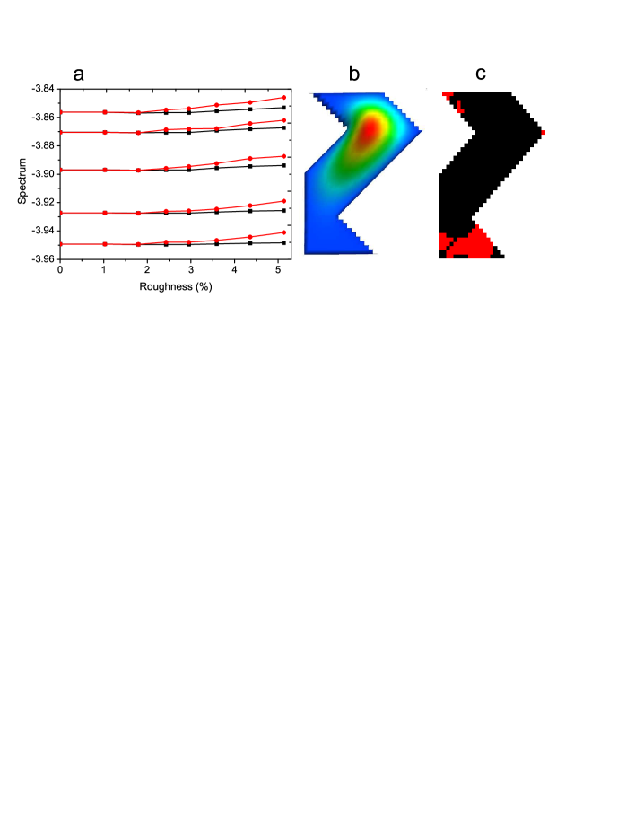
Figure 8: (Color online) a) Spectra evolution of Bilby (black) and Hawk (red) for increasing roughness of edges. b) and c) amplitude and the extracted phase for the first mode of Bilby and a roughness of edges of $3.5\%$. The spectra and amplitude distributions were calculated by averaging over 200 realizations for each roughness. The phase was extracted from the amplitude distributions, with the condition to minimize the misfit after transplantation, as described in text.

IV Conclusions

When one thinks about phase measurements, interference is the first word coming to mind - and it was actually the only word for quite a long time. However, C.R. Moon et.al Science -in a remarkable recent experiment- demonstrated that isospectrality can also be used to extract phase distributions.

In this paper, we have systematically investigated the robustness of such a phase extraction. A certain level of disorder or roughness of edges can compromise the isospectrality-based phase extraction in the same way in which inelastic scattering or environment-induced decoherence can compromise the interferometry-based phase extraction.

Phase extraction in isospectral pairs is possible because the wave functions of the two shapes can be expressed in term of each other by the ”transplantation” procedure. With disorder, the transplantation leads to a misfit of the wave functions, which can be minimized by numerically finding the most suitable phase distribution - called the ”extracted phase”. Our numerical results suggest that, if the misfit is less than $\sim 5\%$, it is likely that the extracted phase is the correct one, i.e. it coincides with the phase in the disorder-free case, which is thereby experimentally available with a certain robustness. If the disorder consists in roughness of edges, the phase extraction is compromised by a roughness exceeding $2.5\%$.

The existence of isospectral shapes is a high exception RMP and the experimental realizations of such shapes at the nanoscale bring supplementary challenges Science . In this context, our proof that the phase extraction can be performed even under imperfect conditions (quantitative estimations were given) may hopefully motivate further experimental realizations.

We explicitly present in the paper numerical results corresponding to averaging over a large number of Anderson disorder configurations or roughness of edges realizarions.

A discrete model is used, which is the natural approach for disorder analysis, allowing also an easy tailoring of any shape. A proof is provided that isospectrality holds in the discrete representation, if some general conditions are fulfilled (see Appendix A).

Another result we obtain is that isospectrality is preserved (in the limit of statistical fluctuations) if the Bilby and Hawk spectra are averaged over a large number of Anderson disorder configurations. On the contrary, if the average is performed over many configurations of edge roughness, isospectrality is lifted if the roughness exceeds $2.5\%$.

V Acknowledgements

We acknowledge support from PN-II, Contract TE 90/05.10.2011 and Core program 45N/2009.

Appendix A Transplantation procedure for the discrete Bilby and Hawk

In this Appendix, we prove the isospectrality of the discrete Bilby and Hawk using the transplantation method Science ; RMP . The adaptation of the method to the discrete case requires some care due to the non-locality of the tight-binding Hamiltonian coming from the hopping terms and, in particular, a transplantation procedure for the triangles border wave functions will be supplementary needed (see Eq. A6). Each of the two shapes is divided into 7 triangles that are labeled as $\alpha$=A,B,…,G for the Bilby drum and as n=1,2,…,7 for the Hawk drum (see Figs.1,9).

The idea of transplantation is to build a valid eigenfunction of, say, Hawk, using an eigenfunction of Bilby. This automatically would prove the one-to-one correspondence of all eigenfunctions (a bijection), and it will also be shown that they correspond to the same energy - implying isospectrality. Fig.9 shows schematically how the transplantation works. An eigenfunction of Hawk is built as follows (in triangle 1, chosen for exemplification): one adds the Bilby function from triangles A and F and substracts the function from triangle E. The triangles in Fig.9 have the borders drawn in three different colors, the rule being simple: neighboring borders of two adjacent triangles must have the same color. The significance of this rule lies in the continuity conditions at borders. Then, algebraic summation of the wave functions from different triangles is performed respecting the ”orientation”. For this purpose, the triangles A and F are simply rotated in plane, but the triangle E must also be flipped once, and as a consequence its wave function is considered with the sign ”-”. The full transplantation recipe, including the rules for the triangles borders, is given in Eqs. A5 and A6. A legitimate question of the reader would be why consider this particular recipe ? It is because it creates indeed valid Hawk eigenfunctions, verifying $H_{Ha}f_{Ha}=Ef_{Ha}$, as will be proven below. It is beyond our purpose here to give a general transplantation recipe for any pair of isospectral shapes, another example can be found in Science , for the Aye-Aye and Beluga shapes, that are devised in 21 triangles each, etc. It goes without saying that only the pairs of isospectral shapes allow such transplantation recipes of building the eigenfunctions of one shape from the other’s eigenfunctions (the existence of a transplantation recipe, that also does not modify the corresponding eigenenergy automatically implies isospectrality).

The transplantation relations allow also the phase calculation. In ”perfect” conditions, if one can measure the amplitude of the eigenmodes inside the triangles $|A|$, $|B|$,…$|G|$ and also $|1|$, $|2|$,…,$|7|$, then one can use the supplementary relations given by the transplantation rules $|A-E+F|=|1|$,……,$|-C+D-F|=|7|$ , to extract uniquely also the phases of the eigenfunctions in the triangles $A$,$B$, .. ,$G$. In particular, the eigenfunctions can be chosen real and the phase is in fact either $0$ or $\pi$, corresponding to positive or negative sign, respectively (see also the discussion in Section II and in reference Science ). In ”imperfect” conditions, however, the equalities $|A-E+F|=|1|$, etc… can only be approximately obeyed, and what one does is to numerically search for the phase distributions that minimize the misfit (defined in Eq.2) between the wave functions calculated by transplantation and those directly measured. In this paper we simulate the imperfect conditions by introducing disorder or edge roughness with the purpose to investigate the robustness of the phase extraction.

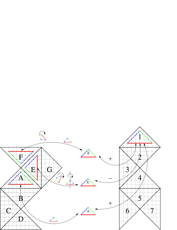
Figure 9: (Color online) The Hawk eigenfunction in triangle 1 - chosen as example in this plot- , can be expressed as a combination of parts from the corresponding eigenfunction of Bilby, by adding the function in triangles A and F and substracting the function in E.

In the discrete model the borders between triangles contain a given number of sites, and they have to be considered explicitly. The borders are named with the pair ”$\alpha\beta$” meaning the border between the triangle $\alpha$ and $\beta$ of Bilby, or ”nm” meaning the border between the triangles n and m of Hawk. First, we write explicitly the two Hamiltonians writing the parts corresponding to the seven triangles, to the borders between triangles and the borders-triangles hopping. The Bilby Hamiltonian can be written:

$$H_{Bi}=\sum_{\alpha=A,..,G}H_{\alpha}+\frac{1}{2}\sum_{(\alpha,\beta)}H_{\alpha\beta}+\sum_{(\alpha,\beta)}(H_{\alpha\rightarrow\alpha\beta}+h.c.),$$ (3)

Where $H_{\alpha}$ is the triangle Hamiltonian that describes the sites inside the triangle $\alpha$ and the hopping between them (borders excluded), $H_{\alpha\beta}$ describes the sites on the border $\alpha\beta$ (the factor $1/2$ ensures that every border is considered once, $H_{\alpha\beta}=H_{\beta\alpha}$). The last term $H_{\alpha\rightarrow\alpha\beta}$ describes the hopping between the triangle $\alpha$ and the border $\alpha\beta$ (for $(\alpha,\beta)$ neighboring triangles). The points on the exterior borders are considered to have infinite potential and need not be included explicitly in the Hamiltonian. Consequently, a wave function of Bilby, corresponding to a certain eigenenergy E, can be written:

$$f_{Bi}=\sum_{\alpha=A,..,G}f_{Bi}^{\alpha}+\frac{1}{2}\sum_{(\alpha,\beta)}f_{Bi}^{\alpha\beta},$$ (4)

and we have:

$$H_{Bi}~{}f_{Bi}=E~{}f_{Bi}.$$ (5)

In the same way the Hawk Hamiltonian is:

$$H_{Ha}=\sum_{n=1,..,7}H_{n}+\frac{1}{2}\sum_{(n,m)}H_{nm}+\sum_{(n,m)}(H_{n\rightarrow nm}+h.c.).$$ (6)

Now we start the transplantation procedure meaning that we build an eigenfunction for Hawk $f_{Ha}$ using a combination of parts from the Bilby eigenfunction $f_{Bi}$ defined in Eq.A2. For simplicity we denote by $\alpha$ and $\alpha\beta$ the triangle and border Bilby wave function $f_{Bi}^{\alpha}$ and $f_{Bi}^{\alpha\beta}$. Similarly, ”n” and ”nm” refer to the triangles and borders projection of the Hawk function $f_{Ha}$.

Now we continue with the full transplantation recipe for our case. The wave functions in the triangles $n=1,2,...,7$ of Hawk can be built from the Bilby triangle functions as follows (the transplantation matrix is the same as for the continuous case Science ; RMP ):

$$\left(\begin{array}[]{c}1\\ 2\\ 3\\ 4\\ 5\\ 6\\ 7\\ \end{array}\right)=\left(\begin{array}[]{ccccccc}1&0&0&0&-1&1&0\\ 0&1&0&0&0&-1&-1\\ 0&0&1&0&-1&0&1\\ -1&0&0&1&0&0&-1\\ 0&-1&0&-1&-1&0&0\\ -1&1&-1&0&0&0&0\\ 0&0&-1&1&0&-1&0\\ \end{array}\right)\left(\begin{array}[]{c}A\\ B\\ C\\ D\\ E\\ F\\ G\\ \end{array}\right),$$ (28)

where, for instance, $"1"$ refers to the Hawk triangle wave function $f_{Ha}^{1}=P_{1}f_{Ha}$, $P_{1}$ being the projection operator on the triangle ”1”, $"A"$ refers to the triangle A of Bilby, etc.

For the border wave functions we define the following transplantation recipe:

$$\left(\begin{array}[]{c}12\\ 23\\ 34\\ 45\\ 56\\ 57\\ \end{array}\right)=\left(\begin{array}[]{cccccc}1&0&0&0&0&-1\\ 0&1&0&0&-1&0\\ 0&0&1&-1&0&0\\ -1&0&0&0&0&-1\\ 0&0&-1&-1&0&0\\ 0&-1&0&0&-1&0\\ \end{array}\right)\left(\begin{array}[]{c}AB\\ BC\\ CD\\ AE\\ EF\\ EG\\ \end{array}\right),$$ (47)

where $"12"$ refers to the triangle wave function $f_{Ha}^{12}=P_{12}f_{Ha}$, $P_{12}$ being the projection operator on the border ”12”. The above relation results from the general rules (A5) considering that the wave functions vanish on the external borders. The transplantation matrix for the border wave function has the dimension $6$ equal to the number of internal triangle borders.

When performing the operations (A5) and (A6), it is important to respect the ”paper folding” principle, exactly as in the continuous case Berard ; Chapman ; RMP . For the first (A5) equation, this means that one has to (imaginary) fold the triangle E over the triangle A on the common border and extract in each point from the triangle A wave function the corresponding triangle E function that landed upon it after the folding, etc.

In the following we have to prove that the Hawk wave function $f_{Ha}$ as described in Eq. (A5) and (A6) is a proper wave function of the Hamiltonian $H_{Ha}$ , and corresponding to the same energy E as in Eq.(A3). For this purpose, we apply the Hawk Hamiltonian (A4) to the transplantated wave function. The proof is a bit lengthly to be written in totality, but rather straightforward. Let us consider for instance the projection on triangle labeled ”1” of $H_{Ha}f_{Ha}$:

$$P_{1}H_{Ha}f_{Ha} = H_{1}f_{Ha}^{1}+H_{12\rightarrow 1}f_{Ha}^{12}$$

$$= H_{1}(f_{Bi}^{A}-f_{Bi}^{E}+f_{Bi}^{F})+H_{12\rightarrow 1}(f_{Bi}^{AB}-f_{Bi}^{EG}).$$

On the other hand on the Bilby shape we have:

$$a) H_{A}f_{Bi}^{A}+H_{AE\rightarrow A}f_{Bi}^{AE}+H_{AB\rightarrow A}f_{Bi}^{AB}=Ef_{Bi}^{A},$$ (49)

$$b) H_{E}f_{Bi}^{E}+H_{EG\rightarrow E}f_{Bi}^{EG}+H_{EF\rightarrow E}f_{Bi}^{EF}+H_{AE\rightarrow E}f_{Bi}^{AE}=Ef_{Bi}^{E},$$

$$c) H_{F}f_{Bi}^{F}+H_{EF\rightarrow F}f_{Bi}^{EF}=Ef_{Bi}^{F}.$$

Now we have to extract Eq.A8(b) from Eq.A8(a) and add Eq.A8(c). The necessary ingredient for isospectrality is that all triangle Hamiltonians are identical: $H_{1}\equiv H_{2}\equiv...H_{7}\equiv H_{A}\equiv...\equiv H_{G}$, and also those corresponding to similar borders and borders-triangles hopping: $H_{12}\equiv H_{AB}$, $H_{12\rightarrow 1}\equiv H_{AB\rightarrow A}$, etc.

The desired result is obtained:

$$P_{1}H_{Ha}f_{Ha}=Ef_{Ha}^{1}.$$ (50)

For the other triangles and for the borders the proof runs identically, therefore one can write:

$$H_{Ha}f_{Ha}=Ef_{Ha}.$$ (51)

One should notice that the isospectrality proof given here is rather general and does not depend on the particular choice of the discrete lattice (as the discrete square network used in our numerical calculation). The only condition is the mentioned equivalence of sub-systems Hamiltonians.

Appendix B Comparison between discrete and continuous models

As shown in the Appendix A, the discrete Bilby and Hawk are isospectral for any discrete representation (see the general conditions in Appendix A). So there is no need to approach the continuous limit (by increasing the number of sites) in order to achieve isospectrality. Still, it is instructive to show that the continuous limit is approached relatively easy, if one aims to study the first few energy levels (there is no need for very many sites or a high computing power). One possible criterium for approaching the continuous limit satisfactory can be a similar spectral structure for the first few energy levels of interest. In other words, the ratio between level spacings should be very close to the corresponding ratio for the continuous model.

In Fig.10 we plot the first six level spacings divided by the first (energy distance between eigenvalues $1^{st}$ and $2^{nd}$). One can see that, for N=13 the ratios are already very close for discrete and continuous models, while for N=21, the difference is even less, as expected. N=13 corresponds to 217 sites on each shape, and N=21 to 641 sites sites . The continuous spectrum was taken from Wu ; Driscoll .

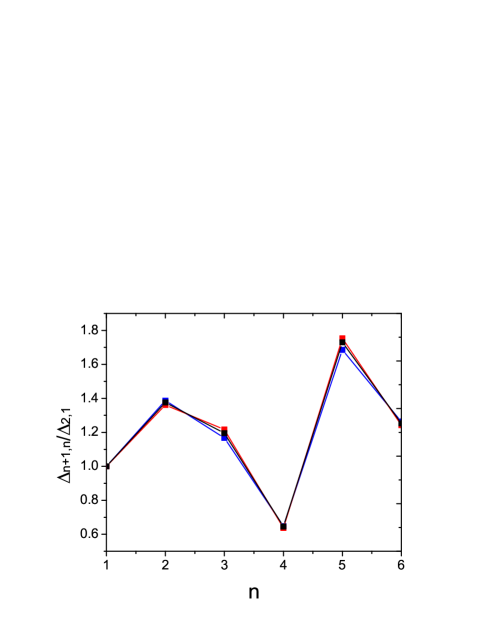
Figure 10: (Color online) The ratio between level spacings $\Delta E_{n,n+1}/\Delta E_{1,2}$ (of the Bilby-Hawk isospectral shapes) is plotted versus the eigenvalue index $n$. The red (light gray) line corresponds to the continuous model, the blue (dark gray) and black lines correspond to the discrete model with $N=13$ and $N=21$, respectively.

Some more comments can be made regarding the comparison between discrete and continuous models. In Marian , it is shown that the discrete and continuous models give the very same result also for dynamical quantities, such as the time-dependent magnetization. The technical difference between continuous and discrete models consist in the the approximations made: in the continuous model a finite number of (analytically known) triangle modes are used to compute the Bilby-Hawk spectrum, while in our discrete approach a finite number of sites is used for the discretization of space. The discrete model is more suitable for implementation of disorder (as we do in this paper) or -eventually- the electron-electron interaction, as we plan to do in a future work. Also, the discrete model allows for easy tailoring of any shapes, without the need of analytical knowledge of sub-systems spectra. The discrete model is also particularly suitable for the simulation of the experimental phase extraction procedure as in Moon et. al Science .

References

- (1) M. Kac, Am. Math. Mon. 73, 1 (1966).
- (2) C. Gordon, D. Webb, S. Wolpert, Inventiones Math. 110, 1 (1992).
- (3) O. Giraud, K. Thas, Rev.Mod.Phys. 82, 2213 (2010).
- (4) H. Wu, D.W.L. Sprung, and J. Martorell, Phys.Rev.E 51, 703 (1995).
- (5) T.A. Driscoll, SIAM Rev. 39, 1 (1997).
- (6) S. Sridhar and A. Kudrolli, Phys.Rev.Lett. 72, 2175 (1994).
- (7) T.A. Driscoll and and H. P. W. Gottlieb, Phys. Rev. E 68, 016702 (2003).
- (8) J.S. Dowker, J. of Phys. A: Math. Gen. 38, 4735 (2005).
- (9) M. Levitin, L. Parnovski, I. Polterovich, J. of Phys. A: Math. Gen. 39, 2073 (2006).
- (10) Christopher R. Moon, Laila S. Mattos, Brian K. Foster, Gabriel Zeltzer, Wonhee Ko, Hari C. Manoharan, Science 319, 782 (2008).
- (11) R. Schuster, E. Buks, M. Heiblum, D. Mahalu, V. Umansky, H. Shtrikman, Nature 385, 417 (1997).
- (12) Y. Oreg, New J. Phys. 9, 122 (2007).
- (13) C. Karrasch, T. Hecht, A. Weichselbaum, Y. Oreg, J. von Delft, and V. Meden, Phys.Rev.Lett. 98, 186802 (2007).
- (14) M. Avinun-Kalish, M. Heiblum, O. Zarchin, D. Mahalu, and V. Umanski, Nature 436, 529 (2005).
- (15) M. Goldstein, R. Berkovits, Y. Gefen, and H.A. Weidenmüller, Phys. Rev. B 79, 125307 (2009).
- (16) M. Ţolea, M. Niţă, A. Aldea, Physica E 42, 2231 (2010).
- (17) M. Rontani, Phys. Rev. B 82, 045310 (2010).
- (18) V.I. Puller, Y. Meir, Phys. Rev. Lett. 104, 256801 (2010).
- (19) S.S. Buchholz, S.F. Fischer, U. Kunze, M. Bell, D. Reuter, and A.D. Wieck, Phys. Rev. B 82, 045432 (2010).
- (20) E.R. Racec, arXiv:1105.1167 (2011).
- (21) The interference method can be regarded as measuring the relevant phases of the scattering eigenmodes, while the isospectrality method determines the phase distribution of the eigenmodes on a surface. In this respect, the difference is basically between the measured systems.
- (22) The total number of sites (for both Bilby and Hawk), corresponding to sites on the hypothenusis of an elementary triangle is: . Notice that, in our model, an odd value is assumed for . For instance in Fig.1 we have corresponding to internal points (the points on the external borders are not counted, as they have infinite potential).
- (23) S. Gnutzmann, U. Smilansky and N. Sondergaard, J. Phys. A: Math. Gen. 38, 8921 (2005).
- (24) M. Niţă, A. Aldea, J. Zittartz, J. Phys.: Condens. Matter 19, 226217 (2007).
- (25) S.J. Chapman, Am. Math. Monthly 102, 124 (1995).
- (26) P. Berard, Math. Ann. 292, 547 (1992).
- (27) S.S. Gylfadottir, M. Niţă, V. Gudmundsson, A. Manolescu, Physica E 27, 278 (2005).