Asymptotic normality of integer compositions inside a rectangle

Abstract

Among all restricted integer compositions with at most $m$ parts, each of which has size at most $l$, choose one uniformly at random. Which integer does this composition represent? In the current note, we show that underlying distribution is, for large $m$ and $l$, approximately normal with mean value $\frac{ml}{2}$.

1 Introduction

An integer composition of a nonnegative integer $n$ is, informally, a way of writing $n$ as a sum of nonnegative integers $\pi_{1},\dotsc,\pi_{k}$, for some $k\geq 0$. Let $h_{l,m}(n)$ denote the number of integer compositions of the nonnegative integer $n$ with at most $m$ parts, each of which has size at most $l$ (‘compositions inside a rectangle’). Recently, Sagan (2009) [14] has shown that the sequence

$$h_{l,m}:=\bigl{(}\,h_{l,m}(0),\dotsc,h_{l,m}(lm)\,\bigr{)},$$

is unimodal. In Figure 1, we plot this sequence for $l=2$, $m=5$; $l=6$, $m=5$; and $l=6$, $m=20$.

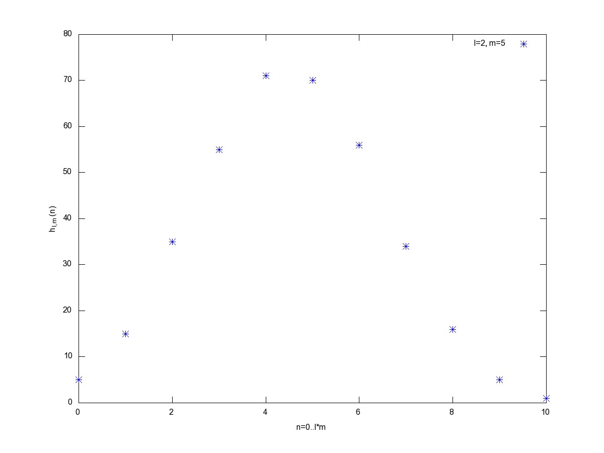
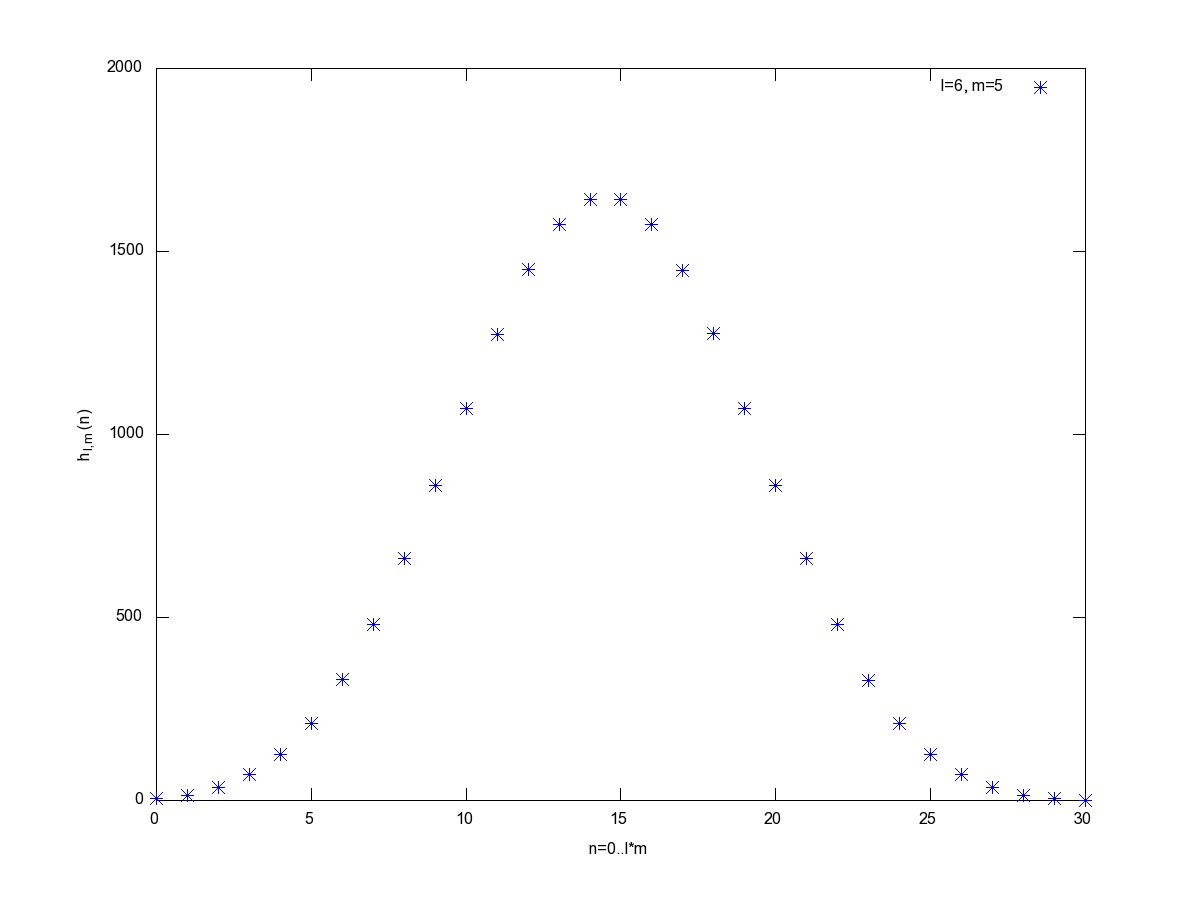
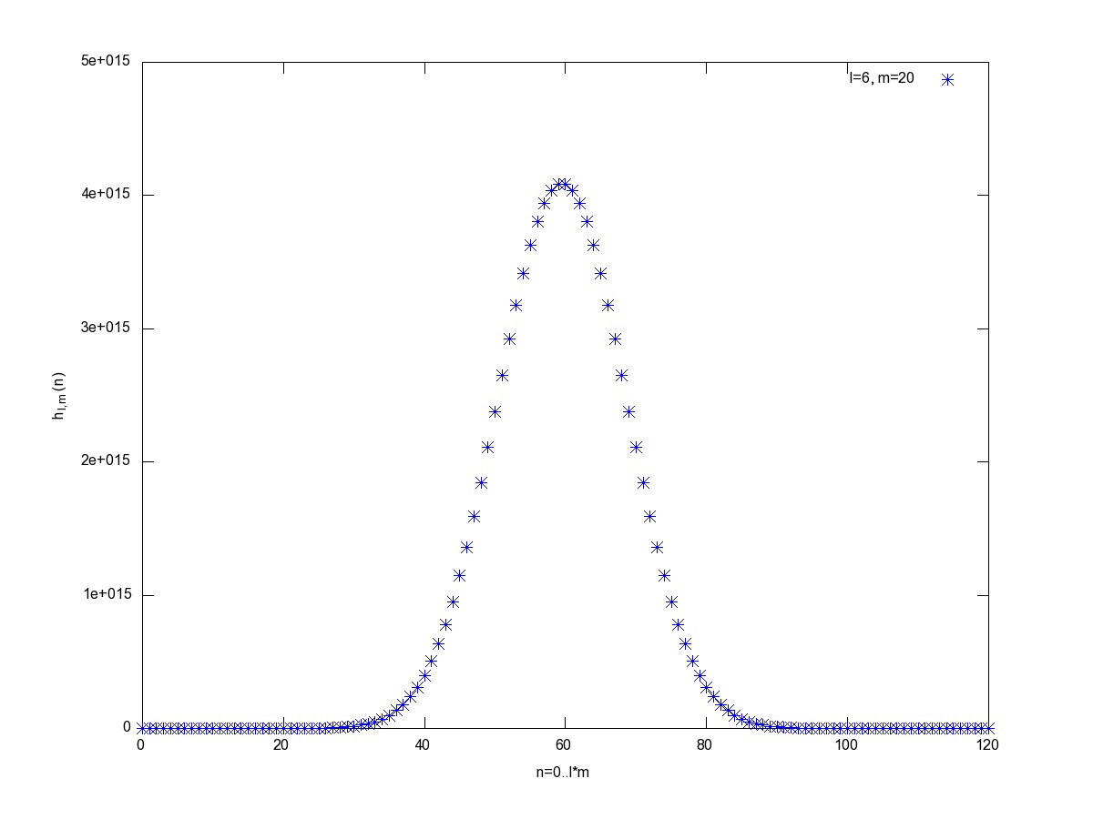
Figure 1: The sequences $h_{l,m}(0),\dotsc,h_{l,m}(lm)$ for $l=2$, $m=5$ (left), $l=6$, $m=5$ (middle) and $l=6$, $m=20$ (right).

Apparently, as $l$ and $m$ increase, $h_{l,m}$ looks more and more ‘Gaussian’. This suggests a probabilistic interpretation of $h_{l,m}(n)$, according to which the normalized values $\frac{h_{l,m}(n)}{\sum_{i=0}^{lm}h_{l,m}(i)}$, $n=0,\dotsc,lm$, denote the probabilities that a uniform randomly chosen integer composition with at most $m$ parts, each of which has size at most $l$, represents the integer $n$. In the current note, we show that these probabilities follow, for large $l$ and $m$, approximately a normal distribution with mean value $\frac{lm}{2}$ and variance $m\frac{(l+1)^{2}-1}{12}$.

Thereby, we first define multinomial triangles as a generalization of Pascal’s triangle and characterize their entries, polynomial coefficients, as generalizations of the well-studied binomial coefficients (Section 2), whereupon we outline a recently found relationship between polynomial coefficients and specificially restricted integer compositions (Section 3). The latter, with various types of restrictions, have attracted much attention in recent years (cf. [2], [4], [8], [10], [13], [15], [16]). For example, Malandro [13] determines asymptotic formulas for $L$-restricted integer compositions — $L$ being an arbitrary finite set — and Shapcott [16] and Schmutz and Shapcott [15] find a lognormal distribution for part products of restricted integer compositions. Hitczenko and Stengle [11] derive the expected number of distinct part sizes of unrestricted random compositions. Restricted and unrestricted integer compositions have a variety of applications, ranging from the theory of patterns [9] to monotone paths in two-dimensional lattices ([12]), alignments between strings ([7]), and the distribution of the sum of discrete integer-valued random variables ([5]).

Then, in Section 4, we state our main theorem, asymptotic normality of compositions inside a rectangle, which we prove in Section 5. In the conclusion, we discuss generalizations of the analyzed setting where part sizes are restricted to lie within arbitrary finite sets.

While our main result, perceived rightly, might be considered not very surprising, the steps that lead to it (Lemmas 5.1 to 5.5) may be judged interesting on their own (and are certainly novel) because they specify the exact distribution of the random variable $X_{l,m}$ that sums the parts of a randomly chosen integer composition from a rectangle of size $l\times m$, and give an elegant characterization of it in terms of the distribution of the sum of independent uniform random variables and an “error term” that quadratically tends toward zero.

2 Multinomial triangles and polynomial coefficients

In generalization to binomial triangles, $(l+1)$-nomial triangles, $l\geq 0$, are defined in the following way. Starting with a $1$ in row zero, construct an entry in row $k$, $k\geq 1$, by adding the overlying $(l+1)$ entries in row $(k-1)$ (some of these entries are taken as zero if not defined); thereby, row $k$ has $(kl+1)$ entries. For example, the monomial ($l=0$), binomial ($l=1$), trinomial ($l=2$) and quadrinomial triangles ($l=3$) start as follows,

1

1

1

1

1
1	1
1	2	1
1	3	3	1

1
1	1	1
1	2	3	2	1
1	3	6	7	6	3	1

1
1	1	1	1
1	2	3	4	3	2	1
1	3	6	10	12	12	10	6	3	1

In the $(l+1)$-nomial triangle, entry $n$, $0\leq n\leq kl$, in row $k$, which we denote by $\binom{k}{n}_{l+1}$ and refer to as polynomial coefficient (cf. Caiado (2007) [1], Comtet (1974) [3]), has the following interpretation. It is the coefficient of $x^{n}$ in the expansion of

$$(1+x+x^{2}+\dotsc+x^{l})^{k}=\sum_{n=0}^{kl}\binom{k}{n}_{l+1}x^{n}.$$ (2.1)

Also note that, by its definition, $\binom{k}{n}_{l+1}$ satisfies the following recursion

$$\binom{k}{n}_{l+1}=\sum_{j=0}^{l}\binom{k-1}{n-j}_{l+1}.$$ (2.2)

3 Integer compositions and polynomial coefficients

An integer composition of a nonnegative integer $n$ is a tuple $\pi=(\pi_{1},\dotsc,\pi_{k})$, $k\geq 0$, of nonnegative integers such that

$$n=\pi_{1}+\dotsc+\pi_{k}$$

where the $\pi_{i}$’s are called parts, and $k$ is the number of parts. Let $\mathcal{C}(n,k,a,b)$ denote the set of restricted compositions of $n$ into $k$ parts $\pi_{i}$ with $a\leq\pi_{i}\leq b$, where $a,b\in\mathbb{N}\cup\{\infty\}$ such that $0\leq a\leq b$, and let $c(n,k,a,b)$ denote its size, $c(n,k,a,b)=\left\lvert\mathcal{C}(n,k,a,b)\right\rvert$. For example, for $n=5$, $k=2$, $a=0$, $b=\infty$, we have

$$5=5+0=0+5=4+1=1+4=3+2=2+3,$$

and thus $c(5,2,0,\infty)=6$.

The following results are well-known.

$$c(n,k,0,\infty) =\binom{n+k-1}{k-1}$$ (3.1)

$$c(n,k,1,\infty) =\binom{n-1}{k-1}$$ (3.2)

$$c(n,k,a,\infty) =c(n-ka,k,0,\infty)=\binom{n-ka+k-1}{k-1}.$$ (3.3)

Moreover, in recent work, Eger (2012) [4] has shown, more generally, a simple relationship between the number of restricted integer compositions and polynomial coefficients, namely,

$$c(n,k,a,b) =\binom{k}{n-ka}_{b-a+1}.$$ (3.4)

4 Main theorem

Let $m$ be a positive integer and let $l$ be a nonnegative integer. Denote by $h_{l,m}(n)$ the number of integer compositions of the integer $n$ with at most $m$ parts $p$, each of which has size at most $l$, i.e. $0\leq p\leq l$. Let $X_{l,m}$ be the random variable that takes on the integer $n$, for $0\leq n\leq lm$, with probability

$$\frac{h_{l,m}(n)}{\sum_{i=0}^{lm}h_{l,m}(i)}.$$

Theorem 4.1.

Let $\mu_{l,m}=\frac{ml}{2}$ and let $\sigma_{l,m}^{2}=\frac{(l+1)^{2}-1}{12}$. Then

$$\frac{X_{l,m}-m\mu_{l,m}}{\sigma_{l,m}\sqrt{m}}\rightarrow\mathcal{N}(0,1)\quad\text{as }l,m\rightarrow\infty.$$

Our strategy for proving Theorem 4.1 is as follows. First, we determine the exact distribution of $X_{l,m}$ in Lemma 5.1. Then we derive the exact distribution of the sum of $m$ independently and uniformly distributed random variables in Lemma 5.2, which is, by the Central Limit Theorem, asymptotically a normal distribution. Next, Lemmas 5.3 and 5.4 provide inequalities and upper bounds that we require in Lemma 5.5, where we show that the distribution of $X_{l,m}$ can be represented, roughly, as the sum of two parts: the distribution of the sum $S_{1}+\dotsc+S_{m}$ of $m$ independently distributed uniform random variables (derived in Lemma 5.2) and an “error term” that converges quadratically toward zero in $l$.

5 Proof of the main theorem

Lemma 5.1.

Let $i$, $1\leq i\leq m$, be the smallest index such that $n\leq il$. Then,

$$P[X_{l,m}=n]=\frac{1}{(l+1)^{m}-1}\frac{l}{l+1}\sum_{j=i}^{m}\binom{j}{n}_{l+1}.$$

Proof.

By definition, $h_{l,m}(n)=\sum_{j=1}^{m}c(n,j,0,l)=\sum_{j=1}^{m}\binom{j}{n}_{l+1}$, where the last equality follows from (3.4). Moreover, $c(n,j,0,l)$ is obviously zero when $j<i$ since $n>(i-1)l$. Finally, the number of integers representable by $j$ parts, each between $0$ and $l$, is obviously $(l+1)^{j}$. Therefore,

$$\sum_{i=0}^{lm}h_{l,m}(i)=\sum_{i=0}^{lm}\sum_{j=1}^{m}c(i,j,0,l)=\sum_{j=1}^{m}\sum_{i=0}^{lm}c(i,j,0,l)=\sum_{j=1}^{m}(l+1)^{j}=\frac{l+1}{l}{\bigl{(}(l+1)^{m}-1\bigr{)}}.$$

Hence,

$$P[X_{l,m}=n]=\frac{h_{l,m}(n)}{\sum_{i=0}^{lm}h_{l,m}(i)}=\frac{1}{(l+1)^{m}-1}\frac{l}{l+1}\sum_{j=i}^{m}\binom{j}{n}_{l+1}.$$

∎

Lemma 5.2.

Denote by $S^{(m)}_{l}$ the sum $S_{1}+\dotsc+S_{m}$ of independent uniform random variables $S_{j}$, $j=1,\dotsc,m$, each taking values from the set $\{0,\dotsc,l\}$. The distribution of $S^{(m)}_{l}$ is given by

$$P[S^{(m)}_{l}=n]=\Bigl{(}\frac{1}{l+1}\Bigr{)}^{m}\binom{m}{n}_{l+1}.$$

Proof.

See Caiado [1], Eger [5]. ∎

Remark 5.1.

Note that the expected value and the variance of $S_{l}^{(m)}$ in Lemma 5.2 are given by

$$\operatorname{E}[S^{(m)}_{l}]=m\operatorname{E}[S_{j}]=\frac{ml}{2},\quad\quad\operatorname{Var}[S^{(m)}_{l}]=m\operatorname{Var}[S_{j}]=m\frac{(l+1)^{2}-1}{12}.$$

Also note that, by the Central Limit Theorem, the distribution of $S_{l}^{(m)}$ is asymptotically normal.

Now, we prove a fact well-known for binomial coefficients, namely, that the ‘central’ coefficient majorizes the remaining coefficients in a given row in the (multinomial) triangle.

Lemma 5.3.

Let $k\geq 0$ and $l\geq 0$ be integers. For all integers $n$ such that $0\leq n\leq kl$,

$$\binom{k}{n}_{l+1}\leq\binom{k}{\lfloor\frac{kl}{2}\rfloor}_{l+1}.$$

Proof.

By the representation of $\binom{k}{n}_{l+1}$ as $\binom{k}{n}_{l+1}=\sum_{j=0}^{l}\binom{k-1}{n-j}_{l+1}$ we find for $n\geq 1$

$$\binom{k}{n}_{l+1}=\binom{k}{n-1}_{l+1}+\Bigl{[}\binom{k-1}{n}_{l+1}-\binom{k-1}{n-l-1}_{l+1}\Bigr{]}.$$ (5.1)

Moreover, it is easy to show that polynomial coefficients are symmetric in the following sense,

$$\binom{k}{n}_{l+1}=\binom{k}{kl-n}_{l+1}.$$

Therefore it suffices to show that the sequence $\binom{k}{0}_{l+1},\binom{k}{1}_{l+1},\dotsc,\binom{k}{\lfloor\frac{kl}{2}\rfloor}_{l+1}$ is non-decreasing. But by (5.1) this easily follows inductively, using the row number $k$ as induction variable. Importantly, note that, in (5.1), if $n\leq\lfloor\frac{kl}{2}\rfloor$, then $\binom{k-1}{n}_{l+1}$ is defined and greater than zero for all $k\geq 2$ since then $n\leq\lfloor\frac{kl}{2}\rfloor\leq(k-1)l$. ∎

In the following lemma, we write $a_{k}\sim b_{k}$ as a short-hand for $\lim_{k\rightarrow\infty}\frac{a_{k}}{b_{k}}=1$. Also note that the following lemma is a generalization of Stirling’s approximation to the central binomial coefficient.

Lemma 5.4.

For all fixed $l$,

$$\binom{k}{\lfloor\frac{kl}{2}\rfloor}_{l+1}\sim\frac{(l+1)^{k}}{\sqrt{2\pi k\frac{(l+1)^{2}-1}{12}}}.$$

Proof.

See Eger [6]. ∎

Lemma 5.5.

For all $l$ and $m$ and for all $n$ such that $0\leq n\leq ml$,

$$P[X_{l,m}=n]=\gamma_{l,m}P[S^{(m)}_{l}=n]+e_{l,m},$$

where $e_{l,m}$ is an “error term” that satisfies

$$0\leq e_{l,m}\leq O(l^{-2})$$

and $\gamma_{l,m}$ satisfies

$$\gamma_{l,m}=\bigl{(}1+O(l^{-1})\bigr{)}^{-1}.$$

Proof.

Let $i$, $1\leq i\leq m$, be the smallest index such that $n\leq il$. Moreover, define $\alpha_{l,m}$ as $\alpha_{l,m}=\frac{1}{(l+1)^{m}-1}\frac{l}{l+1}$ and note that $\alpha_{l,m}=\gamma_{l,m}\frac{1}{(l+1)^{m}}$, where $\gamma_{l,m}=(1+1/l)^{-1}$ (ignoring the $(-1)$ in the denominator of $\alpha_{l,m}$). Then

$$P[X_{l,m}=n] =\alpha_{l,m}\sum_{j=i}^{m}\binom{j}{n}_{l+1}=\alpha_{l,m}\binom{m}{n}_{l+1}+\alpha_{l,m}\sum_{j=i}^{m-1}\binom{j}{n}_{l+1}=\gamma_{l,m}P[S^{(m)}_{l}=n]+e_{l,m},$$

where we define $e_{l,m}=\alpha_{l,m}\sum_{j=i}^{m-1}\binom{j}{n}_{l+1}$. Obviously, $e_{l,m}\geq 0$. Moreover, by Lemmas 5.3 and 5.4

$$e_{l,m} \leq\alpha_{l,m}\sum_{j=i}^{m-1}\binom{j}{\lfloor\frac{jl}{2}\rfloor}_{l+1}\leq\alpha_{l,m}O(1)\sum_{j=i}^{m-1}\frac{(l+1)^{j}}{\sqrt{2\pi j\frac{(l+1)^{2}-1}{12}}}.$$ (5.2)

Now,

$$\frac{(l+1)^{j}}{\sqrt{2\pi j\frac{(l+1)^{2}-1}{12}}}=O(1)\cdot\frac{(l+1)^{j}}{\sqrt{j\bigl{(}(l+1)^{2}-1\bigr{)}}},$$

so that

$$\sum_{j=i}^{m-1}\frac{(l+1)^{j}}{\sqrt{2\pi j\frac{(l+1)^{2}-1}{12}}}=\sum_{j=i}^{m-1}O(1)\frac{(l+1)^{j}}{\sqrt{j}\sqrt{(l+1)^{2}-1}}\leq O(1)\sum_{j=i}^{m-1}(l+1)^{j-1}=O(1)\frac{(l+1)^{i-1}\bigl{[}(l+1)^{m-i}-1\bigr{]}}{l},$$

whence, continuing from (5.2),

$$\begin{split}e_{l,m}&\leq\alpha_{l,m}O(1)\sum_{j=i}^{m-1}\frac{(l+1)^{j}}{\sqrt{2\pi j\frac{(l+1)^{2}-1}{12}}}\leq O(1)\frac{(l+1)^{i-2}}{(l+1)^{m}-1}\bigl{[}(l+1)^{m-i}-1\bigr{]}\\ &\leq O(1)\Bigl{(}(l+1)^{-2}-(l+1)^{i-m-2}\Bigr{)}\leq O(1)(l+1)^{-2}.\end{split}$$ (5.3)

∎

In Table 1, we show the decrease of $e_{l,m}$ in Lemma 5.5 as $l$ increases. Obviously, our bound is apparently quite well, as in fact $e_{l,m}$ seems to approximately quadratically decay in $l$. In Figure 2, the distributions of $X_{l,m}$ and $S_{l}^{(m)}$ for different values of $l$ and $m$ are plotted. The variable $X_{l,m}$ has a particular distributional shape that can be inferred from the proof of Lemma 5.5. For small values $n$ the distribution of $X_{l,m}$ tends to be larger than that of $S_{l}^{(m)}$ — $e_{l,m}$ is relatively larger as can be seen from Equation (5.3) — while this relation is reversed for large $n$.

	$m=10$		$m=20$
$l=1$	$0.0471$		$0.0240$
$l=2$	$0.0191$	$2.46$	$0.0093$	$2.57$
$l=4$	$0.0064$	$2.94$	$0.0031$	$2.96$
$l=8$	$0.0019$	$3.25$	$9.5016\times 10^{-4}$	$3.30$
$l=16$	$5.5909\times 10^{-4}$	$3.56$	$2.6494\times 10^{-4}$	$3.58$
$l=32$	$1.4871\times 10^{-4}$	$3.75$	$7.0291\times 10^{-5}$	$3.76$
$l=64$	$3.8399\times 10^{-5}$	$3.82$	$1.8126\times 10^{-5}$	$3.87$

Table 1: Maximum over absolute differences $\bigl{\lvert}P[X_{l,m}=n]-P[S^{(m)}_{l}=n]\bigr{\rvert}$, $n=0,\dotsc,lm$, for $m=10$ and $m=20$ and varying $l$. We also specify the factor of decrease in these differences between successive $l$ values.

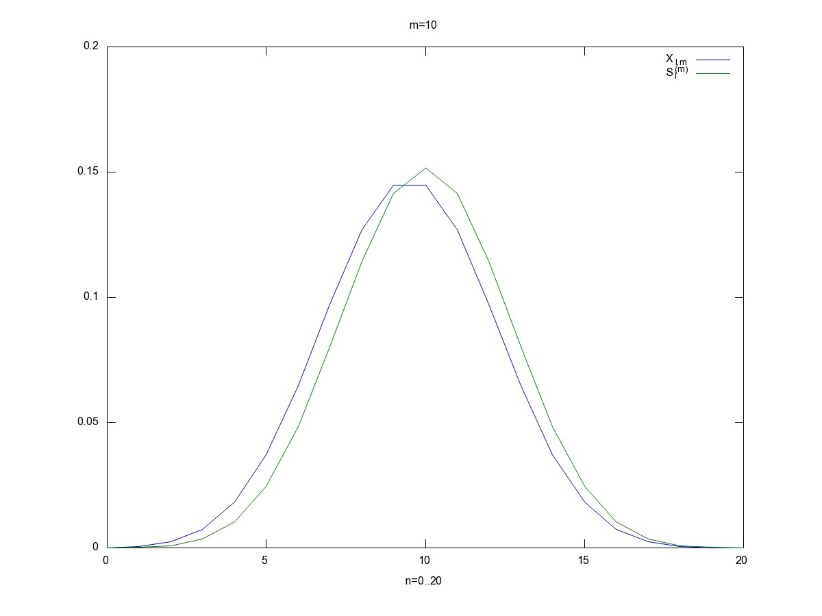
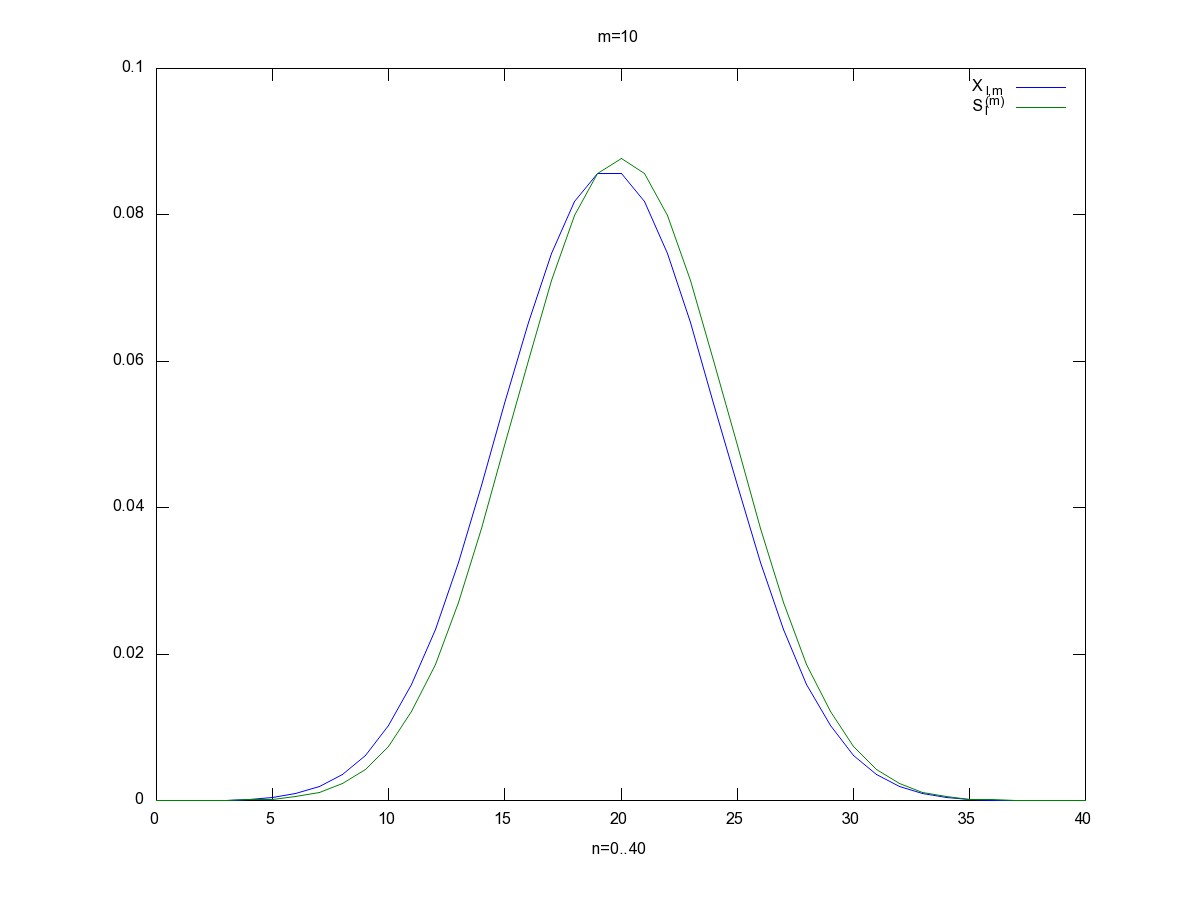
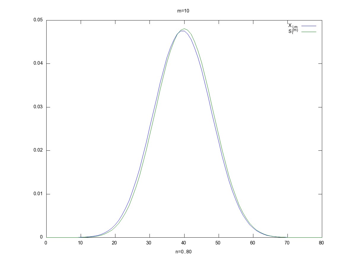
Figure 2: The distributions of $X_{l,m}$ and $S^{(m)}_{l}$ for $m=10$ and $l=2$ (left), $l=4$ (middle), and $l=8$ (right).

6 Conclusion

The choice of the restrictions $0\leq p\leq l$ for parts $p$ of integer compositions has, although illustrating a model case, largely been arbitrary. In fact, similar results as Theorem 4.1 would hold for any finite set $L=\{a_{1},\dotsc,a_{k}\}$ as range for part sizes. For $L=\{a,a+1,\dotsc,b\}$, $0\leq a\leq b$, we find simple closed form solutions of the asymptotic distribution of $X_{L,m}$, where we define $X_{L,m}$ (and other variables such as $S_{L}^{(m)}$) as a generalization of $X_{l,m}$ above with $X_{l,m}=X_{\{0,\dotsc,l\},m}$. For example, in this case, $S^{(m)}_{L}$ has exact distribution

$$\Bigl{(}\frac{1}{b-a+1}\Bigr{)}^{m}\binom{m}{n-ma}_{b-a+1},$$

(cf. Eger (2012) [5]) with expected value $\frac{m(a+b)}{2}$ and is, by the Central Limit Theorem, asymptotically normally distributed. Conversely, the distribution of $X_{L,m}$ allows a similar representation as in Lemma 5.1, as a sum of quantities $\binom{j}{n-ja}_{b-a+1}$ and a normalizing term, from which we can straightforwardly derive a decomposition of $X_{L,m}$ as in Lemma 5.5, with bounds obtained from Lemmas 5.3 and 5.4.

As a final remark, note that our results entail a ‘Stirling’ like formula for $h_{l,m}(n)$. By definition $P[X_{l,m}=n]=\frac{h_{l,m}(n)}{\sum_{i=0}^{lm}h_{l,m}(i)}$, and equating this quantity at its asymptotic mean value $\frac{ml}{2}$ with the corresponding normal density leads to

$$h_{l,m}(\frac{ml}{2})\sim\frac{\bigl{(}(l+1)^{m}-1\bigr{)}\frac{l+1}{l}}{\sqrt{2\pi m\frac{(l+1)^{2}-1}{12}}}.$$

References

- [1] Caiado, C.C.S., and Rathie, P.N. (2007). Polynomial Coefficients and Distribution of the Sum of Discrete Uniform Variables, in Mathai, A. M., Pathan, M. A. Jose, K. K. and Jacob, J., eds., Eighth Annual Conference of the Society of Special Functions and their Applications, Pala, India, Society for Special Functions and their Applications.
- [2] Chinn, P., and Heubach, S. (2003). -compositions. Congressus Numerantium, 164: 183–194.
- [3] Comtet, L. (1974). Advanced Combinatorics, D. Reidel Publishing Company.
- [4] Eger, S. (2012). Integer compositions and multinomial triangles, submitted.
- [5] Eger, S. (2012). Integer compositions and the distribution of discrete random variables, submitted.
- [6] Eger, S. (2012). Stirling’s approximation for central polynomial coefficients, submitted.
- [7] Eger, S. (2012). Sequence alignment with arbitrary steps and further generalizations, with an application to letter-to-sound alignments, submitted.
- [8] Heubach, S., and Mansour, T. (2004). Compositions of with parts in a set. Congressus Numerantium, 164: 127–143.
- [9] Heubach, S., and Mansour. T. (2006). Avoiding patterns of length three in compositions and multiset permutations. Adv. in Appl. Math. 36(2), 156–174.
- [10] Hitczenko, P., and Banderier, C., to appear. Enumeration and asymptotics of restricted compositions having the same number of parts, Discrete Applied Mathematics.
- [11] Hitczenko, P., and Stengle, G. (2000). Expected number of distinct part sizes in a random integer composition. Combin. Probab. Comput., 9(6), 519–527.
- [12] Kimberling, C. (2001). Enumeration of paths, compositions of integers, and Fibonacci Numbers, The Fibonacci Quarterly 39(5).
- [13] Malandro, M.E. (2011). Asymptotics for restricted integer compositions. Preprint available at http://arxiv.org/pdf/1108.0337v1.
- [14] B.E. Sagan, Compositions Inside a Rectangle and Unimodality, Journal of Algebraic Combinatorics 29 (2009), 405–411.
- [15] Schmutz, E., and Shapcott, C. (2011). Part-products of -restricted integer compositions, submitted.
- [16] Shapcott, C. Dissertation (in preparation). PhD thesis, Drexel University.