Accurate fundamental parameters and detailed abundance patterns from spectroscopy of 93 solar-type Kepler targets

Abstract

We present a detailed spectroscopic study of 93 solar-type stars that are targets of the NASA/Kepler mission and provide detailed chemical composition of each target. We find that the overall metallicity is well-represented by Fe lines. Relative abundances of light elements (CNO) and $\alpha$ elements are generally higher for low-metallicity stars. Our spectroscopic analysis benefits from the accurately measured surface gravity from the asteroseismic analysis of the Kepler light curves. The $\log g$ parameter is known to better than 0.03 dex and is held fixed in the analysis. We compare our $T_{\rm eff}$ determination with a recent colour calibration of $V_{\rm T}-K_{\rm S}$ (TYCHO $V$ magnitude minus 2MASS $K_{\rm S}$ magnitude) and find very good agreement and a scatter of only 80 K, showing that for other nearby Kepler targets this index can be used. The asteroseismic $\log g$ values agree very well with the classical determination using Fe i-Fe ii balance, although we find a small systematic offset of $0.08$ dex (asteroseismic $\log g$ values are lower). The abundance patterns of metals, $\alpha$ elements, and the light elements (CNO) show that a simple scaling by [Fe/H] is adequate to represent the metallicity of the stars, except for the stars with metallicity below $-0.3$, where $\alpha$-enhancement becomes important. However, this is only important for a very small fraction of the Kepler sample. We therefore recommend that a simple scaling with [Fe/H] be employed in the asteroseismic analyses of large ensembles of solar-type stars.

1 Introduction

The Kepler Space Mission, launched by NASA on 7 March 2009, has the goal of detecting transiting exoplanets down to Earth-size around solar-type stars (Borucki et al., 2010). The photometric transit depth provides a direct measure of the ratio of the planet-to-star radii. Hence, accurate measurements of the absolute planet radii depend on having robust measurements of the stellar radii. While “classical” methods of stellar radius determination suffer from large uncertainties, radii can be determined to a few percent from asteroseismic modelling of the averaged stellar pulsation data (Stello et al., 2009; Gai et al., 2011). Thus, the exquisite Kepler data (Gilliland et al., 2010; Jenkins et al., 2010) fuel an interesting synergy between exoplanet science and asteroseismology.

Asteroseismology is a powerful tool to sound the stellar interiors and determine their basic properties, such as radius, mass and age (see e.g., Aerts, Christensen-Dalsgaard & Kurtz 2010; Christensen-Dalsgaard & Thompson 2011 and references therein). Much recent progress has been made with ground-based spectroscopy and the CoRoT photometry space missions, with solar-like oscillations detected in a few dozen stars (Michel et al., 2008; Bedding, 2011). The Kepler mission is a major step forward, with oscillations having been detected during an asteroseismic survey in several hundred solar-type stars (Chaplin et al., 2011). More than 150 of these stars have since been observed continuously, the expectation being that a sizable fraction will be monitored for the entire duration of the mission. This will make it possible to investigate stars with convective cores and stars with extensive outer convective envelopes. Reliable measurements of the stars’ fundamental properties firmly constrain the range of models and allows us to exploit the seismic data much more fully (Brown et al., 1994; Basu, Chaplin & Elsworth, 2010). For example, the uncertainty in the measurement of the stellar radius drops from about 40 percent to less than 3 percent when the average large frequency spacing (the frequency between mode frequencies with the same degree and consecutive order of the pulsation modes) is combined with spectroscopic measurements of $T_{\rm eff}$ and metallicity ([Fe/H]). The technique described by Basu, Chaplin & Elsworth (2010) requires an accuracy in the spectroscopic parameters better than about 200 K in $T_{\rm eff}$ for main sequence stars and 0.2 dex in [Fe/H] for more evolved stars. For the detailed theoretical modelling, such accurate parameters are critical for removing the degeneracy between mass and metallicity.

The Kepler Input Catalogue (KIC) (Brown et al., 2011) contains estimates of the parameters of the stars, determined by calibrating $griz$ + Mg $b$ Sloan filter photometry of all stars in the 105 square degree field observed by Kepler. The precision of the KIC parameters has been called into question by recent spectroscopic analyses (Molenda-Żakowicz et al., 2011; Bruntt, Frandsen & Thygesen, 2011). It has been found that $T_{\rm eff}$ only agrees within about 300 K, while $\log g$ can be off by 0.5 dex, and [Fe/H] by up to 2.0 dex. The previous study by Molenda-Żakowicz et al. (2011) reported spectroscopic results on a wide range of stars, from solar-type to A-stars, which relied on medium-resolution spectra and with relatively low signal-to-noise ratio (S/N). In the current study we focus on the FGK (solar-type) stars, using spectra with high S/N (200 or more) and high resolution ($R=80,000$). This enables us to measure accurate values for $T_{\rm eff}$ and to obtain a detailed abundance pattern for each star.

2 Observations and data reduction

The spectra were obtained with the ESPaDOnS spectrograph at the 3.6-m Canada-France-Hawaii Telescope (CFHT) (Donati et al., 2006) in USA and with the NARVAL spectrograph mounted on the 2-m Bernard Lyot Telescope at the Pic du Midi Observatory in France. In both facilities the observations were carried out as service observations from May to September in 2010. The two spectropolarimetric instruments are very similar and we used the “star mode” with a nominal resolution of $R=80\,000$. The integration times were typically a few minutes up to 15 minutes and were adjusted to obtain S/N ratios in the range 200 to 300 per pixel. Here, we report results for the 93 stars that have detections of solar-type oscillations in the Kepler light curve data. An additional 20 stars, which are evolved stars ($\log g<3.5$), will be presented by Thygesen et al. (in preparation). However, these stars are included here in our calibration of $T_{\rm eff}$ and microturbulence.

We have used the standard pipeline-reduced spectra (Donati et al., 1997), in which the overlapping part of the échelle orders have not been merged. We used the program called rainbow (Bruntt et al., 2010b) to normalize the spectra manually. We carefully adjusted the continua by comparing with a synthetic spectrum calculated with the program that was used for the spectral line fitting. We made sure the overlapping part of the orders agreed on both the line depths and the level of the continuum. A few of the stars were observed on different nights with both spectrographs and we confirmed that their spectra were very similar. In these cases we used the spectrum with the highest S/N ratio in the continuum around 6000 Å. One star, KIC 8379927 (HD 187160), was not included in the analysis because it is an double-lined spectroscopic binary (Griffin, 2007). In addition, two stars (KIC 12155015 and 8831759) were found to be too cool ($T_{\rm eff}$ $<$4500 K) for detailed analysis.

3 Data analysis

We used the semi-automatic software VWA (Bruntt et al., 2010a) to derive fundamental stellar parameters and elemental abundances from the spectra. This software has been used to analyse several of the CoRoT exoplanet host stars (Bruntt et al., 2010b) and asteroseismic targets (Bruntt, 2009), and the results compared well with other methods, including interferometric determinations of the effective temperature (Bruntt et al., 2010a). It has also been demonstrated that the $\log g$ determination is accurate for nearby binary systems (Bruntt et al., 2010a), including Procyon and $\alpha$ Cen A+B.

VWA treats each line individually and fits them by iteratively changing the abundance and calculating synthetic profiles. VWA automatically takes into account any line blending. This makes it possible to analyse the F-type stars in the sample, which have wide lines with $v\sin i$ in the range 10 to 40 km s^-1, as well as cool stars ($T_{\rm eff}$$>$ 4500 K) where blending becomes severe in the blue part of the spectrum. We have extracted the atomic line lists from the VALD database (Kupka et al., 1999), using the appropriate $T_{\rm eff}$ and $\log g$ of each star. This is important in order for the line depths computed by VALD to be approximately correct. In addition, we updated the atomic line parameters in the region around the lithium line at 6707 Å, using the line list from Ghezzi et al. (2009), but we note that our code cannot take into account the weak CN molecular bands.

VWA uses atmospheric models that are interpolated in a grid of MARCS models (Gustafsson et al., 2008) for a fixed microturbulence of 2 km s^-1. We tested that changing to 1 km s^-1 had a negligible effect on the results. The grid had a mesh size of 250 K for $T_{\rm eff}$, 0.5 for $\log g$, and variable for [Fe/H], with a step size of typically 0.25 dex around the solar value. Abundances in MARCS models were all scaled relative to the solar abundance from Grevesse, Asplund & Sauval (2007).

Table 1: Atomic data used in the spectra analysis. The wavelength, excitation energy and oscillator strengths ($\log gf$) from VALD and the adjusted values are given. We list C,N, and O and the complete table is available in the electronic version.

		Excitation	VALD	Adjusted
El.	$\lambda$ $[$Å$]$	$[$eV$]$	$\log gf$	$\log gf$
C i	$4932.049$	$7.685$	$-1.884$	$-1.070$
	$5052.167$	$7.685$	$-1.648$	$-1.196$
	$5380.337$	$7.685$	$-1.842$	$-1.475$
	$5800.602$	$7.946$	$-2.338$	$-2.075$
	$6010.675$	$8.640$	$-4.605$	$0.031$
	$6014.834$	$8.643$	$-1.585$	$-1.379$
	$6397.961$	$8.771$	$-1.778$	$-1.287$
	$6587.610$	$8.537$	$-1.596$	$-0.901$
	$6655.517$	$8.537$	$-1.370$	$-1.669$
	$7111.469$	$8.640$	$-2.140$	$-0.209$
	$7113.179$	$8.647$	$-0.774$	$-0.700$
	$7115.168$	$8.643$	$-0.935$	$-0.808$
	$7116.988$	$8.647$	$-0.508$	$0.093$
	$7119.657$	$8.643$	$-1.149$	$-0.785$
	$8058.624$	$8.851$	$-1.275$	$-0.907$
	$8335.148$	$7.685$	$-0.420$	$-0.117$
N i	$7442.300$	$10.330$	$-0.384$	$-0.030$
	$7468.313$	$10.336$	$-0.189$	$0.137$
	$8629.240$	$10.690$	$0.075$	$0.670$
	$8683.405$	$10.330$	$0.086$	$0.527$
	$8711.707$	$10.330$	$-0.234$	$0.139$
O i	$5577.339$	$1.967$	$-8.204$	$-7.726$
	$6156.776$	$10.741$	$-0.694$	$-0.109$
	$6158.186$	$10.741$	$-0.409$	$-0.113$
	$6300.304$	$0.000$	$-9.819$	$-10.268$
	$7002.229$	$10.989$	$-1.855$	$-0.165$
	$7771.941$	$9.146$	$0.369$	$0.820$
	$7774.161$	$9.146$	$0.223$	$0.642$
	$7775.390$	$9.146$	$0.001$	$0.357$

3.1 Analysis of solar spectra

VWA relies on a differential approach, with a solar spectrum as the reference, in order to correct for systematics in the atmospheric models and to minimize errors in the atomic oscillator strengths. We adopted the new version of the Fourier Transform Spectrometer (FTS) Kitt Peak Solar Flux Atlas (Kurucz, 2006), which was also adopted by Asplund et al. (2009). This spectrum is a new reduction of the original spectrum obtained by Kurucz et al. (1984). When we compared the FTS spectrum with the calculated spectrum for the canonical solar values of $T_{\rm eff}=5777$ K and $\log g=4.437$, we found that the continuum of the synthetic profiles lies at 1.0 but the FTS spectrum is generally somewhat lower, especially in the blue part of the spectrum. This is probably due to the many “missing lines” in present-day line compilations. Since abundances are derived from the synthetic spectra, we re-normalized the FTS spectrum to have the same continuum level (close to 1.0) as the synthetic spectrum of the Sun. We used the same normalization approach for all the Kepler targets.

To remove instrumental effects, one option would be to use a solar spectrum observed with the same instrument as for the observations. The reason for adopting the FTS spectrum is its superior quality compared to what can be obtained through a normal calibration spectrum with an échelle spectrograph. The FTS spectrum has a resolution of about $R=300\,000$ and a S/N of about 3000. We were thus able to determine oscillator strength ($\log gf$) corrections for more than 1200 lines in the range 4500 to 9200 Å. Secondly, the FTS instrument design serves to minimize scattered light, which is known to affect échelle spectra. In Table 1 we list atomic data for lines that were used in at least 10 of the Kepler targets. The complete table is available in the electronic version.

Table 2: Properties of observed solar spectra. The $\Delta{\rm[Fe/H]}$ is the mean offset in Fe abundance between the FTS spectrum and the other spectra and $N$ is the number of spectral lines used.

Spectrograph	Source of light	$\Delta{\rm[Fe/H]}$	$N$
FTS	Direct	$\equiv 0.00$	405
ESPaDOnS	Twilight Sky	$-0.04\pm 0.04$	284
NARVAL	Moon	$-0.03\pm 0.04$	276
HARPS	Moon	$-0.02\pm 0.04$	197
HARPS	Ceres	$-0.02\pm 0.03$	214
FIES	Day Sky	$-0.05\pm 0.06$	280
HERMES	Venus	$-0.06\pm 0.07$	347

To investigate the influence of the adopted FTS solar spectrum, we analysed several spectra of the Sun taken with the spectrographs used for the Kepler stars: NARVAL and ESPaDOnS. In addition, we also analysed solar spectra from different spectrographs, including HARPS at the La Silla 3.6-m telescope, FIES at the 2.56-m Nordic Optical Telescope, and HERMES at the 1.2-m MERCATOR telescope. The solar spectra we acquired by observing scattered sunlight either from twilight or daytime sky, or by observing the Moon, Ceres or Venus.

In Table 2 we list the seven solar spectra we have analysed. We used lines in the range 4500 to 6800 Å and equivalent widths from 5 to 105 mÅ. Typically between 200 and 300 lines were used in each spectrum, depending on the S/N. When measuring abundances of each line relative to the FTS spectrum, we found a very slight correlation with wavelength, presumably due to insufficient removal of scattered light. In addition, we found that the spectral lines were weaker in all spectra compared to the FTS, giving lower abundances by 0.03 – 0.07 dex. In Table 2 we list the offset for Fe i and note that offsets are nearly identical for the other elements. This is expected if the cause is dilution of the lines by scattered light. We recommend that in future analyses, a spectrum of the Sun is always acquired to estimate the maximum error that is due to scattered light. From our spectra from NARVAL and ESPaDOnS we measured abundances that are 0.03 and 0.04 dex too low. We have therefore added 0.03 dex to the abundances of all stars.

4 Spectral analysis of Kepler targets

In the initial spectral analysis of the Kepler stars we used fixed starting parameters, namely $T_{\rm eff}=6000$ K, $\log g=4.0$ and $v_{\rm micro}=1.0$ km s^-1. The $v\sin i$ was adjusted manually by comparing synthetic spectra to isolated lines in the range 6000 – 6150 Å. Values for macroturbulence were taken from the calibration of Bruntt et al. (2010a). The final $v\sin i$ was adjusted later, once the other atmospheric parameters had been improved. VWA was run in an automatic mode, where the atmospheric parameters were iteratively adjusted. This was done by minimizing the correlations of the Fe i abundance with both equivalent width (EW) and excitation potential (EP), as described by Bruntt et al. (2010a, b). This was achieved by adjusting $T_{\rm eff}$ and microturbulence. Also, we demanded that Fe i and Fe ii agreed, which is dependent on both $T_{\rm eff}$ and $\log g$. This iterative approach adopted non-local thermodynamical equilibrium (NLTE) corrections to Fe i using interpolations and extrapolations in the figures in Rentzsch-Holm (1996). This is exactly the same approach used in previous analyses with VWA, but in the next section we describe an important change in the analysis, utilizing the asteroseismic results.

Table 3: Observed targets and their properties. The KIC parameters are given in columns 7–9, spectroscopic parameters in columns 9–10, and the final values of $T_{\rm eff}$, $\log g$, [Fe/H], and microturbulence are given in columns 11–14, labelled “asteroseismic $\log g$”. When the asteroseismic $\log g$ is used the uncertainties are: 60 K for $T_{\rm eff}$, 0.03 dex for $\log g$, 0.06 km s^-1 for microturbulence and 0.06 dex for [Fe/H]. For the spectroscopic values, the uncertainties are 0.08 dex for $\log g$ and 70 K for $T_{\rm eff}$. Note that we only list the the “asteroseismic” values of $v\sin i$ and $v_{\rm micro}$, since the “spectroscopic” are almost identical.

						“KIC param.”			“Spect. $\log g$”		“Asteroseismic $\log g$”
KIC-ID	HIP	HD	$V_{\rm T}$	$V_{\rm T}-K_{\rm S}$	$E(B-V)$	$T_{\rm eff}$	$\log g$	[Fe/H]	$T_{\rm eff}$	$\log g$	$T_{\rm eff}$	$\log g$	[Fe/H]	$v_{\rm micro}$	$v\sin i$
						[K]			[K]		[K]			[km s-1]	[km s-1]
1430163			9.627	1.098		6910	3.66	$-0.05$	6574	4.27	6520	4.22	$-0.11$	1.64	11.0
1435467			9.017	1.299	$0.01\pm 0.02$	6570	4.02	$-0.25$	6345	4.24	6264	4.09	$-0.01$	1.45	10.0
2837475		179260	8.547	1.083		6444	4.07	$-0.06$	6740	4.51	6700	4.16	$-0.02$	2.35	23.5
3424541			9.895	1.281		6207	3.58	$-0.12$	6180	3.50	6080	3.82	$0.01$	1.39	29.8
3427720			9.280	1.454	$0.00\pm 0.04$	5780	4.44	$-0.37$	6070	4.51	6040	4.38	$-0.03$	1.16	4.0
3456181			9.776	1.297	$0.03\pm 0.02$	6361	3.54	$-0.66$	6344	4.05	6270	3.93	$-0.19$	1.53	7.8
3632418	94112	179070	8.310	1.365	$0.00\pm 0.04$				6235	4.14	6190	4.00	$-0.16$	1.42	6.5
3656476			9.643	1.635	$0.00\pm 0.04$	5424	4.47	$-0.60$	5720	4.31	5710	4.23	$0.34$	1.02	2.0
3733735	94071	178971	8.409	1.035	$0.02\pm 0.02$	6442	4.03	$-0.62$	6715	4.45	6715	4.26	$-0.04$	1.99	16.8
4586099			9.321	1.341	$0.03\pm 0.02$	6037	3.93	$-0.77$	6296	4.05	6296	4.02	$-0.17$	1.50	6.1
4638884			9.934	1.182		6367	4.07	$-0.31$	6380	4.01	6375	4.03	$-0.03$	1.72	7.8
4914923	94734		9.571	1.636					5880	4.30	5905	4.21	$0.17$	1.19	3.6
5021689			9.588	1.392	$0.01\pm 0.02$	5997	4.29	$-0.32$	6150	4.11	6168	4.02	$-0.08$	1.39	9.8
5184732			8.386	1.565		5599	4.31	$-0.09$	5865	4.38	5840	4.26	$0.38$	1.13	3.3
5371516	96528	185457	8.483	1.281	$0.02\pm 0.02$	6050	4.17	$-0.11$	6408	4.34	6408	3.98	$0.17$	1.61	15.2
5450445			9.880	1.378		5965	4.20	$-0.30$	6110	4.15	6112	3.98	$0.05$	1.36	8.9
5512589			10.229	1.666		5554	4.39	$-0.32$	5780	4.16	5750	4.06	$0.06$	1.11	3.5
5596656			9.867	2.244	$0.00\pm 0.04$	4942	4.29	$-1.43$	5014	3.48	5094	3.35	$-0.46$	0.83	4.0
5773345			9.331	1.385		6009	4.27	$0.08$	6184	4.08	6130	4.00	$0.21$	1.46	6.6
5774694	93657	177780	8.439	1.508					5878	4.66	5875	4.47	$0.07$	1.02	5.2
5939450	92771	175576	7.384	1.284	$0.01\pm 0.02$				6200	3.61	6282	3.70	$-0.18$	1.56	8.3
5955122			9.446	1.527	$0.02\pm 0.02$	5747	4.39	$-0.21$	5865	3.88	5837	3.87	$-0.17$	1.22	6.5
6106415	93427	177153	7.275	1.446	$0.00\pm 0.04$				6055	4.40	5990	4.31	$-0.09$	1.15	4.0
6116048			8.540	1.419	$0.01\pm 0.02$	5863	4.32	$-0.07$	5990	4.32	5935	4.28	$-0.24$	1.02	4.0
6225718	97527	187637	7.580	1.297					6250	4.46	6230	4.32	$-0.17$	1.38	5.0
6442183		183159	8.661	1.678	$0.02\pm 0.02$				5740	4.16	5760	4.03	$-0.11$	1.06	4.5
6508366			9.078	1.277	$0.03\pm 0.02$	6271	4.14	$-0.21$	6310	3.95	6354	3.94	$-0.08$	1.52	18.2
6603624			9.282	1.716	$0.01\pm 0.02$	5416	4.38	$-0.06$	5640	4.47	5625	4.32	$0.28$	1.05	3.0
6679371			8.792	1.192		6313	4.07	$-0.17$	6390	3.91	6260	3.92	$-0.13$	1.62	19.2
6933899			9.818	1.647	$0.01\pm 0.02$	5616	4.25	$-0.09$	5870	4.07	5860	4.09	$0.02$	1.15	3.5
7103006			8.919	1.217		6203	4.26	$-0.01$	6394	4.18	6394	4.01	$0.05$	1.58	13.2
7206837			9.908	1.333		6100	4.15	$-0.23$	6304	4.21	6304	4.17	$0.14$	1.29	10.1
7282890			9.155	1.214	$0.03\pm 0.02$	6072	4.05	$-0.44$	6410	4.11	6384	3.88	$0.02$	1.74	22.6
7510397	93511	177412	7.922	1.378	$0.01\pm 0.02$	5972	4.13	$-0.35$	6130	4.07	6110	4.01	$-0.23$	1.35	5.4
7529180			8.542	1.094		6367	3.52	$-0.43$	6790	4.70	6700	4.23	$-0.02$	1.81	33.6
7662428			9.797	1.888		6088	4.18	$-0.04$	6360	4.35	6360	4.27	$0.22$	1.46	15.7
7668623			9.441	1.286		6013	4.11	$-0.29$	6270	4.01	6270	3.87	$-0.02$	1.43	9.6
7680114			10.227	1.554	$0.02\pm 0.02$	5578	4.63	$-0.33$	5825	4.25	5855	4.18	$0.11$	1.10	3.0
7747078	94918		9.593	1.617	$0.03\pm 0.02$				5910	3.98	5840	3.91	$-0.26$	1.22	6.0
7799349			9.782	2.264		4920	3.47	$0.18$	5065	3.71	5115	3.67	$0.41$	1.21	1.0
7800289			9.599	1.218		6208	4.21	$-0.35$	6389	3.79	6354	3.71	$-0.23$	1.66	21.6
7871531			9.512	1.996	$0.00\pm 0.04$	5153	4.16	$-0.44$	5400	4.43	5400	4.49	$-0.24$	0.71	2.9
7940546	92615	175226	7.477	1.303		5987	4.17	$-0.14$	6240	4.11	6264	3.99	$-0.19$	1.56	9.7
7970740		186306	8.042	1.957	$0.00\pm 0.04$	5231	4.41	$-0.18$	5290	4.57	5290	4.58	$-0.49$	0.68	3.0
7976303			9.220	1.490	$0.01\pm 0.02$	6005	4.23	$-0.59$	6095	4.03	6053	3.87	$-0.53$	1.37	5.5
8006161	91949		7.610	1.940		5184	3.63	$0.36$	5370	4.51	5390	4.49	$0.34$	1.07	2.5
8026226			8.529	1.300	$0.02\pm 0.02$	5930	3.84	$-0.85$	6260	3.80	6230	3.71	$-0.16$	1.58	10.6
8179536			9.570	1.292	$0.02\pm 0.02$	6163	4.12	$-0.20$	6369	4.39	6344	4.27	$0.01$	1.44	9.0
8228742	95098		9.564	1.448	$0.04\pm 0.02$	5858	3.97	$-0.26$	6070	4.00	6042	4.02	$-0.14$	1.30	5.7
8360349		181777	8.719	1.279	$0.00\pm 0.04$	6044	4.21	$-0.09$	6340	4.15	6340	3.81	$0.12$	1.61	17.9
8367710			9.987	1.238		6166	4.31	$-0.01$	6465	4.17	6500	3.99	$0.16$	1.70	21.1
8394589			9.648	1.422		5938	3.82	$-0.33$	6130	4.33	6114	4.32	$-0.36$	1.23	6.0
8524425			9.995	1.818	$0.03\pm 0.02$	5449	3.92	$-0.21$	5620	4.03	5634	3.98	$0.14$	1.23	2.3
8542853			10.382	2.579	$0.00\pm 0.04$	5406	4.41	$-0.15$	5560	4.67	5560	4.54	$-0.20$	0.80	3.5
8561221			10.166	2.076	$0.03\pm 0.02$	4997	4.65	$-0.77$	5300	3.76	5245	3.61	$-0.06$	1.01	3.5
8579578			8.996	1.228	$0.03\pm 0.02$	6078	4.21	$-0.22$	6470	4.27	6380	3.92	$-0.09$	1.92	24.7

Table 3: Observed targets and their properties (table continued)

						“KIC param.”			“Spect. $\log g$”		“Asteroseismic $\log g$”
KIC-ID	HIP	HD	$V_{\rm T}$	$V_{\rm T}-K_{\rm S}$	$E(B-V)$	$T_{\rm eff}$	$\log g$	[Fe/H]	$T_{\rm eff}$	$\log g$	$T_{\rm eff}$	$\log g$	[Fe/H]	$v_{\rm micro}$	$v\sin i$
						[K]			[K]		[K]			[km s-1]	[km s-1]
8694723			8.977	1.314	$0.03\pm 0.02$	6101	4.15	$-0.51$	6200	4.08	6120	4.10	$-0.59$	1.39	6.6
8702606			9.595	1.911	$0.02\pm 0.02$	5308	4.60	$-0.48$	5540	3.92	5540	3.76	$-0.09$	1.08	4.0
8738809			10.133	1.452		5848	4.38	$-0.15$	6090	4.02	6090	3.90	$0.11$	1.33	4.9
8751420	95362	182736	7.103	2.075	$0.00\pm 0.02$				5294	3.80	5264	3.70	$-0.15$	1.00	3.5
8760414			9.752	1.579	$0.02\pm 0.02$				5795	4.25	5787	4.33	$-1.14$	1.03	3.0
8938364			10.287	1.651	$0.00\pm 0.04$	5741	4.34	$-0.38$	5620	4.17	5630	4.16	$-0.20$	1.00	3.8
9098294			9.980	1.616	$0.02\pm 0.02$	5701	4.44	$-0.73$	5770	4.26	5840	4.30	$-0.13$	1.01	4.0
9139151	92961		9.351	1.399	$0.00\pm 0.04$	5911	4.32	$-0.15$	6105	4.54	6125	4.38	$0.11$	1.22	6.0
9139163	92962	176071	8.386	1.155	$0.00\pm 0.04$	6220	4.28	$-0.13$	6375	4.27	6400	4.18	$0.15$	1.31	4.0
9206432	93607		9.152	1.085	$0.01\pm 0.02$	6301	4.27	$-0.06$	6608	4.45	6608	4.23	$0.23$	1.70	6.7
9226926			8.741	1.032	$0.02\pm 0.02$	6735	3.57	$-1.01$	6892	4.49	6892	4.14	$-0.23$	2.04	31.1
9812850			9.576	1.277	$0.01\pm 0.02$	6169	4.21	$-0.29$	6330	4.16	6325	4.05	$-0.16$	1.61	12.9
9908400			9.157	1.332		5823	4.18	$0.04$	6620	4.45	6400	3.74	$0.34$	1.65	26.1
9955598			9.717	1.949	$0.00\pm 0.04$	5333	3.71	$0.19$	5395	4.52	5410	4.48	$0.11$	0.87	2.0
10016239			9.871	1.130		6232	4.29	$-0.58$	6340	4.33	6340	4.31	$-0.05$	1.42	14.7
10018963			8.832	1.379	$0.00\pm 0.04$	5977	4.16	$-0.47$	6130	3.98	6020	3.95	$-0.35$	1.32	5.5
10068307	94675	180867	8.299	1.355	$0.00\pm 0.04$	6052	4.13	$-0.21$	6140	4.00	6114	3.93	$-0.22$	1.38	6.5
10124866	93108	176465	8.674	2.334	$0.00\pm 0.04$	5813	4.24	$-0.14$	5850	4.55	5755	4.48	$-0.30$	0.82	3.0
10162436	97992		8.747	1.389	$0.01\pm 0.02$	6095	4.18	$-0.23$	6180	4.02	6200	3.95	$-0.08$	1.44	6.5
10355856			9.294	1.237	$0.00\pm 0.04$	6288	4.06	$-0.53$	6395	4.12	6350	4.08	$-0.19$	1.55	7.2
10454113	92983		8.744	1.453	$0.00\pm 0.04$	5972	4.30	$-0.11$	6120	4.32	6120	4.31	$-0.06$	1.21	5.5
10462940			9.836	1.368	$0.00\pm 0.04$	6070	4.27	$-0.19$	6174	4.46	6154	4.32	$0.10$	1.29	4.3
10516096			9.611	1.482	$0.02\pm 0.02$	5814	4.19	$-0.31$	5940	4.21	5940	4.18	$-0.06$	1.12	4.2
10644253			9.324	1.450	$0.00\pm 0.04$	5831	4.28	$-0.15$	6105	4.59	6030	4.40	$0.12$	1.14	3.8
10709834			9.859	1.071	$0.00\pm 0.04$	6502	3.99	$-0.23$	6570	4.17	6508	4.09	$-0.08$	1.66	10.6
10923629			9.936	1.300	$0.03\pm 0.02$	5982	4.26	$-0.00$	6214	3.95	6214	3.82	$0.16$	1.50	11.4
10963065			8.893	1.407	$0.01\pm 0.02$	6043	4.16	$-0.25$	6090	4.31	6060	4.29	$-0.20$	1.06	5.4
11026764			9.783	1.921	$0.00\pm 0.04$	5502	3.90	$-0.25$	5670	4.01	5682	3.88	$0.05$	1.17	4.8
11081729			9.061	1.088	$0.02\pm 0.02$	6359	3.98	$-0.10$	6630	4.41	6630	4.25	$-0.12$	1.72	20.0
11137075			11.034	1.760	$0.01\pm 0.02$	5425	4.17	$0.00$	5590	4.30	5590	4.01	$-0.06$	0.96	1.0
11244118			9.937	1.643		5507	4.50	$0.14$	5735	4.23	5745	4.09	$0.35$	1.16	3.0
11253226	97071	186700	8.514	1.055	$0.00\pm 0.02$	6468	4.18	$-0.34$	6605	4.21	6605	4.16	$-0.08$	1.73	15.1
11414712			8.785	1.752	$0.00\pm 0.04$	5388	3.80	$-0.66$	5620	3.84	5635	3.80	$-0.05$	1.18	4.4
11498538	93951	178874	7.420	1.172	$0.03\pm 0.02$	6287	4.04	$-0.30$	6496	3.83	6496	3.76	$0.01$	1.77	38.4
11717120			9.586	2.180	$0.00\pm 0.04$	4980	3.44	$-0.45$	5105	3.80	5150	3.68	$-0.30$	0.98	1.0
12009504			9.380	1.311	$0.00\pm 0.02$	6056	3.70	$0.13$	6125	4.23	6065	4.21	$-0.09$	1.13	8.4
12258514	95568	183298	8.204	1.446	$0.00\pm 0.04$	5808	4.30	$0.09$	6025	4.28	5990	4.11	$0.04$	1.22	3.5

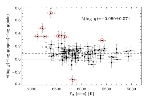
Figure 1: The difference in $\log g$ determined from spectroscopic and asteroseismic methods. The spectroscopic value is systematically higher by about 0.08 dex with RMS scatter of 0.07 dex (dashed line indicates the mean difference). A few apparent outliers have been marked by open symbols and discussed in Sect. 4.1.

4.1 Adopting asteroseismic $\log g$ values

The determination of stellar $\log g$ values from spectroscopy alone is notoriously unreliable. Although internal errors of less than 0.1 dex are often reported from high-quality data, realistic uncertainties are more likely of the order $\pm$0.2 dex (Smalley, 2005). Asteroseismically determined $\log g$ values are significantly more precise. This is due to the measurement of stellar oscillations, whose gross properties (large separation and frequency of maximum amplitude) depend on the mass, radius and effective temperature via well-established scaling relations (Brown, 1991; Kjeldsen & Bedding, 1995). The surface gravity scales as $M/R^{2}$ and is therefore very well determined from asteroseismology (Christensen-Dalsgaard et al., 2010). This allows us to further constrain the other spectroscopically determined parameters. For example, changing $T_{\rm eff}$ affects how Fe i depends on EP and both $\log g$ and $T_{\rm eff}$ affect the Fe i / Fe ii ionization balance, which can lead to a strong correlation of the output parameters of $T_{\rm eff}$ and $\log g$. This was seen in the analysis of the solar-like Kepler target KIC 11026764 reported by Metcalfe et al. (2010), where the $\log g$ uncertainty was reduced from 0.3 dex to 0.02 dex using asteroseismology.

In the present work, we have adopted the same approach of fixing the $\log g$ to the asteroseismically determined values. The asteroseismic $\log g$ were estimated with the grid-based Yale-Birmingham pipeline (Basu, Chaplin & Elsworth, 2010; Gai et al., 2011), which used as input the seismic parameters $\Delta\nu$ and $\nu_{\rm max}$, and the spectroscopically determined $T_{\rm eff}$ and [Fe/H], while adopting the Yonsei-Yale grid of evolution models (see Basu, Chaplin & Elsworth 2010 for details). The seismic parameters came from independent analyses of the Kepler lightcurves performed by five different teams (details are given by Verner et al. 2011a, b).

We found that the difference between different model grids mentioned in Basu, Chaplin & Elsworth (2010) resulted in changes in the estimated $\log g$ of less than 0.02 dex in 90 percent of the stars and less than 0.05 dex for all stars. These are smaller than the typical uncertainties in $\log g$ when determined from the spectrum alone, which are typically 0.08 dex for the slowly rotating stars in the sample, and slightly larger for the moderately fast rotators.

The determined stellar parameters are given in Table 3, both using the “asteroseismic $\log g$” in columns 12–15 and the classical “spectroscopic method” (e.g. as described in Bruntt et al. 2010a) in columns 10–11. For completion we also list the KIC parameters in columns 7–9. The differences in determined parameters between the two methods are generally small, with mean differences and RMS values as follows $\Delta\log g=+0.08\pm 0.07$ dex, $\Delta T_{\rm eff}=+10\pm 38$ K, $\Delta{\rm[Fe/H]}=-0.00\pm 0.03$ dex, and $\Delta v_{\rm micro}=+0.02\pm 0.09$ km s^-1(calculated in the sense “classical” minus seismic). Considering that the error on the mean values is $\sqrt{N}\simeq 9$ times smaller than the RMS values given here, only the difference in $\log g$ is significant (10 $\sigma$), while the differences in $T_{\rm eff}$ and microturbulence are at the $2\,\sigma$ level.

To further investigate the significant discrepancy in $\log g$, we show in Fig. 1 the difference between the $\log g$ found from the two different methods. We see that the difference does not depend on spectral type. We cannot offer an explanation for the systematic offset, but the quite low RMS scatter of 0.07 dex indicates that the two methods are internally consistent. Further analyses are needed to understand these differences. Use of independent estimates, provided by analysing binary stars that also show pulsating solar-type components, would be highly desirable in this context and might be possible in future space missions like PLATO (Catala, 2009). We note that from Fig. 1, the “classical” method appears to be able to determine $\log g$ with an accuracy of about 0.10 dex for solar-type stars.

The stars with large offsets are marked by circles in Fig. 1 and have KIC-IDs: 2837475, 3424541, 5371516, 7529180, 8360349, 8579578, 9226926, 9908400, and 11137075. The last star has parameters close to the Sun but the others have $T_{\rm eff}$ in the range 6080 – 6890 K, $\log g$ from 3.7 to 4.2, and $v\sin i$ between 15 and 34 km s^-1. One star (3424541) has only 2 usable Fe ii lines, while the others have at least 6 and up to 17. We do not find an immediate explanation for these apparent outliers in $\log g$.

In the remainder of this paper we use the stellar parameters from using the asteroseismic $\log g$, and we have labelled the axes in the figures $T_{\rm eff}$ (seis) and $\log g$ (seis).

Figure 2: The upper panel shows $T_{\rm eff}$ (seis) vs. $V_{\rm T}-K_{\rm S}$ for stars with at least 100 Fe i lines. The three stars that lie above the general distribution are close binary systems. The solid line is the fit from Eq. 1 and the dashed line is the fit from Casagrande et al. (2010). The middle and lower panels show the difference in $T_{\rm eff}$ for the two calibrations.

4.2 Photometric calibration of $T_{\rm eff}$

We have used the adopted spectroscopic parameters to make a calibration of $T_{\rm eff}$ vs. the photometric index $V_{\rm T}-K_{\rm S}$, where $V_{\rm T}$ is the TYCHO $V$ magnitude and $K_{\rm S}$ is the 2MASS magnitude. All stars in our sample have measured values of these magnitudes. We adopted this index because it is known to be a very good indicator of $T_{\rm eff}$. For example, Casagrande et al. (2010) found this index to have one of the lowest RMS residuals among the many indices they used for calibrating $T_{\rm eff}$.

In Fig. 2 we plot $T_{\rm eff}$ (seis) vs. the colour index $V_{\rm T}-K_{\rm S}$. The dashed line is the calibration of this index taken from Casagrande et al. (2010) and the residuals from the fit are shown in the middle panel. The offset of 4 K is negligible compared to the RMS scatter of 85 K. The solid line in the top panel is a second order fit and the residuals are shown in the bottom panel, with a slightly lower RMS scatter of 69 K. The three obvious outliers (KIC 7662428, 8542853, and 10124866), which are all close binary systems with near-equal components, have been excluded from the calculations of the fit and the RMS values. The calibration is

$$T_{\rm eff}/{\rm K}=8545-2090\,(V_{\rm T}-K_{\rm S})+250\,(V_{\rm T}-K_{\rm S})^{2}.$$ (1)

This new empirical calibration is valid for both main sequence and sub-giant stars ($\log g>2.5$) with $V_{\rm T}-K_{\rm S}$ in the range $1$ – $3$. The 1-$\sigma$ uncertainty is 70 K, as measured from the RMS scatter.

To estimate the influence of interstellar reddening, we measured the strength of the Na D doublet at $5990+5995$ Å. In 70 stars, interstellar lines were present and their equivalent widths were measured. The strength has been calibrated by Munari & Zwitter (1997) to give $E(B-V)$ with an uncertainty of 0.05 mag. The values we determined are given in Table 3. We find that most stars with a detectable interstellar Na D doublet have almost negligible reddening, with values in the range from 0.00 to 0.06 mag. The two stars with the highest values of $E(B-V)$ are KIC 3430868 and 8491147, which have values of 0.043 and 0.058. Since the calibration has an uncertainty of 0.05 mag, we consider the interstellar reddening to be negligible for most of the targets.

4.3 A new calibration of microturbulence

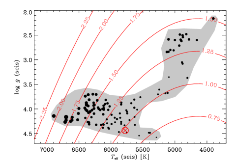
Figure 3: The diagram of $T_{\rm eff}$ (seis) vs. asteroseismic $\log g$ for Kepler targets. The size of the points scale with the microturbulence. The contours show the calibration of microturbulence and the gray area marks the region where it is valid. The location of the Sun is marked with a cross and circle. Stars with $\log g$ below 3.5 are taken from Thygesen et al. (in preparation).

In the final determination of the stellar parameters, $\log g$ was held fixed at the asteroseismically determined value, and only $T_{\rm eff}$ and the microturbulence were allowed to vary. The locations of the stars in the $T_{\rm eff}$ vs. $\log g$ diagram are shown in Fig. 3. We made a set of calibrations of the microturbulence using different combinations of $T_{\rm eff}$ and $\log g$ and found that the following gave the lowest residuals:

$$v_{\rm micro}/{\rm km\,s}^{-1} = 1.095+\,5.44\times 10^{-4}\,(T_{\rm eff}-5700)$$ (2)

$$+\,2.56\times 10^{-7}\,(T_{\rm eff}-5700)^{2}$$

$$-\,0.378\,(\log g-4.0)\,.$$

The RMS scatter of the residuals is 0.095 km s^-1, reducing to 0.057 km s^-1 when a handful of 3-$\sigma$ outliers are removed. A fit without the quadratic term in $T_{\rm eff}$ gives 20% higher residuals. To be conservative, we adopt an uncertainty on this calibration of 0.1 km/s. When using the above calibration, one must include the uncertainties in $T_{\rm eff}$ and $\log g$. For typical uncertainties in $T_{\rm eff}$ of 100 K and 0.1 dex in $\log g$, one finds a total uncertainty in microturbulence of 0.13 km/s. This new calibration is in agreement with that presented by Bruntt et al. (2010a), but has a wider applicability due to the increased sample size. The region of applicability is marked by the grey area in Fig. 3, i.e. roughly 5300 – 6900 K for main-sequence stars and 4500 – 5200 K for the evolved stars ($\log g$ from 2.1 to 3.5).

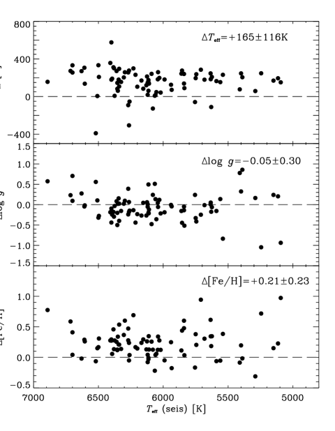
Figure 4: Differences between our adopted spectroscopic parameters ($\log g$ from asteroseismology) and the KIC photometric parameters of $T_{\rm eff}$, $\log g$ and [Fe/H]. The “$\Delta$” means spectroscopic minus KIC parameter. The mean offset and RMS are given in each panel.

5 Comparison with the KIC

Out of 93 stars in our sample, 83 stars have stellar parameters in KIC (Brown et al., 2011). In Fig. 4 we compare our adopted spectroscopic values, i.e. with $\log g$ fixed at the asteroseismically determined value, of $T_{\rm eff}$, $\log g$, and [Fe/H] with the KIC.

In each panel we give the mean offset and RMS scatter. These values were calculated using a robust method where 3-$\sigma$ outliers were removed (3, 4, 2 outliers were removed, respectively). It seems the KIC parameters are quite reliable across the entire spectral range from 5100 to 6900 K, although there is a significant offset in $T_{\rm eff}$ and [Fe/H]. Considering the approach of converting the ground-based photometry to fundamental parameters described by Brown et al. (2011), which includes the non-trivial task of removing sky extinction and interstellar reddening, we verify that the quality of the KIC catalogue is generally very good. Compared to our spectroscopic values, we find that $T_{\rm eff}$ in KIC are 165 K lower and [Fe/H] are 0.21 dex lower.

There is a modest, negative offset between the asteroseismic $\log g$ and the KIC $\log g$ values. This is consistent with the results presented in Verner et al. (2011a), once allowance is made for differences in the samples of stars used. They compared asteroseismic $\log g$ with the KIC $\log g$ of more than 500 Kepler dwarfs and subgiants. They found reasonable agreement between the two sets of values for KIC $\log g<4$, but at progressively higher values the KIC $\log g$ were found to increasingly overestimate the asteroiseismic $\log g$. The average offset, over the entire ensemble, was about 0.17 dex.

Most of the stars in this paper fall in the region $\log g\geq 4$, and the significant offset identified by Verner et al. (2011a) is present in those stars in our sample. However, there are only a few stars in this paper with KIC $\log g<4$, and they all have quite sizeable negative differences with respect to the asteroseismic $\log g$. In contrast, the sampling of stars in Verner et al. having $\log g<4$ was much more comprehensive and showed a mean offset close to zero. The effect of the sparse lower $\log g$ sample here is to reduce the mean offset from $\approx 0.17$ dex to the $\approx 0.05$ dex seen in Fig. 4.

6 Consideration of NLTE effect on Fe i

In Fig. 5 we show the difference in abundance derived from Fe i and Fe ii lines, without applying any NLTE corrections, showing evidence for a correlation with $T_{\rm eff}$. There is a large scatter, but most stars with $T_{\rm eff}>6000$ K have a higher abundance from Fe ii. Indeed, it is predicted by theoretical NLTE calculations for iron that, under the assumption of LTE, the computed Fe i lines will be too strong, hence the abundances determined from Fe i too small. The magnitude of this effect for A- and early F-type stars was computed by Rentzsch-Holm (1996) based on a model of the Fe atom, although recent calculations show that the effect is smaller (Mashonkina et al., 2010, 2011). However, our empirical results appear to be in rough agreement with those of Rentzsch-Holm (1996). As an example, for the hottest stars in our sample (6500 K), $+0.07$ dex is the correction to be applied to Fe i, while extrapolations from the Figures in Rentzsch-Holm (1996) indicate that Fe i  should be adjusted by $+0.05$ dex.

Our analyses are strickly differential with respect to the Sun. Hence, Fe i and Fe ii abundances are expected to agree for stars with similar parameters. In fact, Fig. 5 shows that this is the case for the majority of these stars. Recall from Fig. 1 that there is an apparent increase in the discrepancy in $\log g$ for the hottest stars, which could be the result of NLTE effects. However, the fact that the $\log g$ offset appears to be independent of $T_{\rm eff}$, except for these hotter stars, suggests that this is not a result of NLTE effects alone, but could be due to other effects, such as the shortcomings of mixing-length theory or 1D model atmospheres. It is beyond the scope of this paper to discuss this in more detail and we suggest that a larger sample of Kepler stars, with both asteroseismic $\log g$ values and accurate spectroscopic $T_{\rm eff}$, is needed to place stronger constraints on theoretical NLTE calculations.

Figure 5: Difference in abundances determined from Fe ii and Fe i in 79 unevolved stars using asteroseismic $\log g$ values and without applying any NLTE corrections.

7 The abundance patterns

The distribution of metallicities is presented as a histogram in Fig. 6. Normally one would use Fe i lines, since stellar spectra typically have between 200 and 300 isolated lines for the slowly rotating stars in our sample. However, NLTE effects start to become important for Fe i above 6000 K (Sect. 6). The Fe ii lines are less affected, since singly-ionized iron is the most common state of Fe, and so we used Fe ii as our primary metallicity indicator.

Figure 6 includes only stars with at least 10 Fe ii lines (85 stars). The peak value of the sample was computed from a fit of a Gaussian profile to the histogram (dashed bell-curve in Fig. 6). The central value is $-0.04$ dex with a FWHM of $0.35$ dex. We have used a bin size of 0.05 dex, but we found that changing this in the range 0.02 to 0.10 only changed the mean metallicity by 0.02 dex. Similarly, using Fe i instead we found a mean value of $-0.08$ dex.

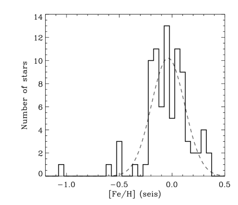
Figure 6: Histogram of the spectroscopically determined iron abundance. The diagram shows [Fe/H] using only Fe ii lines as determined for 85 stars with at least 10 Fe ii lines. The dashed curve is a Gaussian fit. The star with the lowest ${\rm[Fe/H]}=-1.14$ is KIC 8760414.

When performing the asteroseismic analysis of Kepler light curves, one often does not have a reliable estimate of the metallicity. This is a problem when comparing with theoretical evolution grids, especially for evolved stars (Basu, Chaplin & Elsworth, 2010). Based on the distribution of metallicity in Fig. 6, we recommend that for such cases one adopts ${\rm[Fe/H]}=-0.07\pm 0.20$. In our sample, only seven stars have metallicity below $-0.3$ and four stars are above $+0.3$. However, we note that this small sample of stars with “extreme” metallicity will be particularly interesting to study due to their different internal opacity, which may affect the asteroseismic properties of the stars.

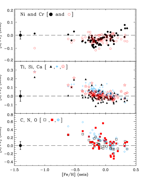
Figure 7: Abundance scaled with Fe versus the Fe abundance for selected elements. The error bar around the solid circle at ${\rm[Fe/H]}=-1.4$ indicates the approximate scatter of the points, which are 0.03, 0.06 and 0.10 dex for the three panels. The dashed horizontal line indicates the solar abundance. Note the different scale in the lower panel.

Table 4: Abundances relative to the Sun and the number of lines used for 13 elements. For each star the first and second line is for the neutral and singly ionized lines, respectively. The adopted uncertainties are 0.07 dex for elements with more than five lines and 0.15 for other elements. The complete table is available in the electronic version.

KIC ID	Li		C		N		O		Na		Mg		Si		Ca		Ti		V		Cr		Fe		Ni
1430163			$-0.09$	$11$	$-0.13$	$2$	$+0.03$	$4$	$-0.14$	$5$	$-0.08$	$2$	$-0.18$	$18$	$-0.13$	$20$	$-0.17$	$10$	$-0.10$	$1$	$-0.17$	$18$	$-0.14$	$233$	$-0.21$	$43$
													$+0.04$	$1$			$-0.13$	$22$			$-0.16$	$13$	$-0.08$	$26$
1435467			$-0.11$	$10$	$+0.51$	$3$	$+0.10$	$5$	$+0.26$	$6$	$-0.04$	$2$	$-0.02$	$13$	$+0.02$	$6$	$-0.11$	$10$	$+0.01$	$1$	$-0.08$	$16$	$-0.04$	$188$	$-0.06$	$21$
											$+0.07$	$2$	$+0.16$	$1$			$+0.04$	$19$			$-0.04$	$11$	$+0.05$	$19$
2837475			$-0.05$	$7$	$-0.31$	$3$	$-0.06$	$1$	$+0.05$	$2$	$-0.06$	$2$	$-0.02$	$14$	$+0.05$	$10$	$+0.01$	$7$		$2$	$-0.13$	$7$	$-0.05$	$133$	$-0.04$	$30$
											$+0.00$	$2$	$-0.09$	$1$			$-0.13$	$8$			$-0.20$	$5$	$-0.05$	$12$
3424541	$+1.44$	1	$+0.34$	$8$	$+0.50$	$2$	$+0.43$	$1$	$+0.15$	$2$	$-0.24$	$1$	$+0.19$	$18$	$+0.17$	$5$	$+0.01$	$6$	$-0.21$	$1$	$-0.06$	$10$	$-0.02$	$69$	$+0.01$	$34$
													$+0.51$	$1$			$+0.25$	$4$			$+0.08$	$4$	$+0.32$	$2$
3427720	$+1.53$	1	$+0.05$	$7$	$-0.07$	$1$	$+0.06$	$2$	$-0.05$	$4$	$+0.04$	$2$	$-0.04$	$28$	$-0.02$	$21$	$-0.08$	$26$	$-0.05$	$5$	$-0.06$	$16$	$-0.06$	$226$	$-0.09$	$63$
											$+0.11$	$1$	$-0.03$	$1$			$+0.04$	$19$			$-0.14$	$7$	$-0.04$	$21$
3430868			$+0.04$	$4$			$+0.02$	$4$	$+0.21$	$2$	$+0.07$	$3$	$0.08$	$21$	$+0.11$	$9$	$+0.02$	$29$	$+0.09$	$11$	$+0.02$	$11$	$+0.06$	$157$	$-0.03$	$44$
																	$+0.09$	$17$			$+0.02$	$8$	$+0.01$	$19$
3456181	$+1.59$	1	$-0.09$	$10$	$+0.01$	$1$	$+0.02$	$5$	$-0.20$	$4$	$-0.15$	$2$	$-0.23$	$24$	$-0.14$	$21$	$-0.24$	$19$	$-0.21$	$3$	$-0.28$	$20$	$-0.22$	$205$	$-0.29$	$45$
													$+0.05$	$1$			$-0.07$	$24$			$-0.25$	$8$	$-0.10$	$30$
3632418			$-0.20$	$11$	$-0.19$	$2$	$+0.08$	$3$	$-0.14$	$6$	$-0.15$	$2$	$-0.17$	$25$	$-0.10$	$19$	$-0.19$	$18$	$-0.23$	$2$	$-0.21$	$20$	$-0.19$	$291$	$-0.22$	$54$
											$-0.10$	$1$	$-0.11$	$1$			$-0.09$	$21$			$-0.22$	$11$	$-0.14$	$29$
3656476			$+0.34$	$12$	$+0.30$	$2$	$+0.16$	$5$	$+0.34$	$4$	$+0.42$	$2$	$+0.28$	$36$	$+0.29$	$9$	$+0.25$	$22$	$+0.29$	$17$	$+0.29$	$10$	$+0.31$	$221$	$+0.30$	$57$
											$+0.39$	$1$	$+0.29$	$1$			$+0.31$	$19$			$+0.20$	$7$	$+0.28$	$17$
3733735			$-0.16$	$12$	$-0.31$	$4$	$+0.01$	$2$	$-0.08$	$3$	$-0.08$	$2$	$-0.04$	$16$	$-0.03$	$18$	$+0.06$	$15$			$-0.11$	$16$	$-0.07$	$147$	$-0.10$	$35$
											$-0.01$	$2$	$-0.01$	$1$			$-0.12$	$20$			$-0.15$	$12$	$-0.07$	$18$

In Fig. 7 we show the abundances of eight important elements versus the metallicity. Ni and Cr have the most lines in the spectra after Fe. Ti, Si and Ca also have many lines and are tracers of the $\alpha$ elements. C, N and O have fewer lines but are important because they directly affect the fusion processes in the core of the star. We only show abundances for stars with at least 5 lines of each element, except for N and O where 2 and 3 lines were considered enough to compute the mean abundance. Also, only stars with $v\sin i$ below 25 km s^-1 are included in the plots. Around 92 and 95 stars are shown in the top and middle panels, respectively, while 35 stars are shown in the bottom plot.

The abundance patterns in Fig. 7 indicate that Fe is a very good proxy for the metals, since the scatter is very low for the 92 stars plotted. The $\alpha$ elements show more scatter and, as expected, the low-metallicity stars have relatively high abundance of these elements. The CNO abundances are more uncertain, since they rely on relatively few lines, but they appear to show the same trend.

It is important to recall that the abundances we have inferred in this work are based on 1D-LTE model atmospheres of the outer $\simeq 1$ per cent of the star. Furthermore, the content of helium cannot be measured, giving further uncertainty to the relative abundances. These surface abundances are assumed to fully represent those of the stellar interior. It can be debated whether the individual abundance patterns of the 13 elements in Table 4 should be used in the asteroseismic modelling. The scatter in the individual abundances shown in Fig. 7 is relatively small. Therefore, we recommend a simple approach, based on scaling the solar abundance with metallicity, except for metal-poor stars. For ensemble asteroseismology (Chaplin et al., 2011) we therefore recommend simply to use Fe  i (or Fe ii for stars hotter than 6000 K) from Table 4 to scale all elements. However, for stars with metallicity in the range $-0.7<{\rm[Fe/H]}<-0.2$, the $\alpha$ elements should be increased by 0.15 dex, and by 0.2 dex for CNO. Population II stars (${\rm[Fe/H]}\la-1.0$) are extremely rare in the Kepler field (we only observed one star KIC 8760414) and for these we recommend using an individually measured abundance pattern.

8 Conclusions

We have used high-precision stellar spectra to analyse the atmospheric properties of 93 solar-type stars that have been observed by Kepler. We have used the spectra to determine the effective temperature, surface gravity and heavy-element abundance of each star. These results will facilitate the asteroseismic investigation by providing accurate fundamental parameters of some of the brightest F5 to K1 type stars of the mission.

We find that the quantity [Fe/H] is sufficient to describe the metallicity of most stars in our sample. The [Fe/H] distribution can be well-represented by a Gaussian with a mean of $-0.06$ dex and FWHM of 0.36 dex.

We confirmed that $\log g$ can be determined in a classical spectroscopic analysis while forcing neutral and ionized lines to give the same abundance. We find a systematic offset of the spectroscopic and asteroseismic $\log g$ of 0.08 dex. Taking this into account, a spectroscopic $\log g$ can be determined with an accuracy of about 0.10 dex for solar-type stars.

We note that the PLATO satellite mission (Catala, 2009), a candidate M-class mission to the ESA Cosmic Vision program, will provide asteroseismic parameters for a very large number of planet-hosting stars. For such a mission, one needs to carefully plan the huge effort needed to obtain ground-based spectroscopy to characterize the targets. Since many of the targets will be fainter than the Kepler targets in this work, it will be necessary to work with low-S/N and/or low-resolution spectra. It will probably be the case that our approach to fix $\log g$ from the asteroseismic data will be essential for the spectroscopic analyses. This could also be true for the characterization of the many remaining Kepler targets with missing spectroscopic parameters $T_{\rm eff}$, [Fe/H], and $v\sin i$.

References

- Aerts, Christensen-Dalsgaard & Kurtz (2010) Aerts C., Christensen-Dalsgaard J., Kurtz D. W., 2010, Asteroseismology. Springer 2010
- Asplund et al. (2009) Asplund M., Grevesse N., Sauval A. J., Scott P., 2009, ARA&A, 47, 481
- Basu, Chaplin & Elsworth (2010) Basu S., Chaplin W. J., Elsworth Y., 2010, ApJ, 710, 1596
- Bedding (2011) Bedding T. R., 2011, ArXiv: 1107.1723
- Borucki et al. (2010) Borucki W. J. et al., 2010, Science, 327, 977
- Brown (1991) Brown T. M., 1991, ApJ, 371, 396
- Brown et al. (1994) Brown T. M., Christensen-Dalsgaard J., Weibel-Mihalas B., Gilliland R. L., 1994, ApJ, 427, 1013
- Brown et al. (2011) Brown T. M., Latham D. W., Everett M. E., Esquerdo G. A., 2011, AJ, 142, 112
- Bruntt (2009) Bruntt H., 2009, A&A, 506, 235
- Bruntt et al. (2010a) Bruntt H. et al., 2010a, MNRAS, 405, 1907
- Bruntt et al. (2010b) Bruntt H. et al., 2010b, A&A, 519, A51
- Bruntt, Frandsen & Thygesen (2011) Bruntt H., Frandsen S., Thygesen A. O., 2011, A&A, 528, A121
- Casagrande et al. (2010) Casagrande L., Ramírez I., Meléndez J., Bessell M., Asplund M., 2010, A&A, 512, A54
- Catala (2009) Catala C., 2009, Experimental Astronomy, 23, 329
- Chaplin et al. (2011) Chaplin W. J. et al., 2011, Science, 332, 213
- Christensen-Dalsgaard et al. (2010) Christensen-Dalsgaard J. et al., 2010, ApJ, 713, L164
- Christensen-Dalsgaard & Thompson (2011) Christensen-Dalsgaard J., Thompson M. J., 2011, in IAU Symposium, Vol. 271, IAU Symposium, N. Brummell, A. S. Brun, M. S. Miesch & Y. Ponty, ed., pp. 32–61
- Donati et al. (2006) Donati J.-F., Catala C., Landstreet J. D., Petit P., 2006, in Astronomical Society of the Pacific Conference Series, Vol. 358, Astronomical Society of the Pacific Conference Series, R. Casini & B. W. Lites, ed., pp. 362–368
- Donati et al. (1997) Donati J.-F., Semel M., Carter B. D., Rees D. E., Collier Cameron A., 1997, MNRAS, 291, 658
- Gai et al. (2011) Gai N., Basu S., Chaplin W. J., Elsworth Y., 2011, ApJ, 730, 63
- Ghezzi et al. (2009) Ghezzi L., Cunha K., Smith V. V., Margheim S., Schuler S., de Araújo F. X., de la Reza R., 2009, ApJ, 698, 451
- Gilliland et al. (2010) Gilliland R. L. et al., 2010, ApJ, 713, L160
- Grevesse, Asplund & Sauval (2007) Grevesse N., Asplund M., Sauval A. J., 2007, Space Sci. Reviews, 130, 105
- Griffin (2007) Griffin R. F., 2007, The Observatory, 127, 313
- Gustafsson et al. (2008) Gustafsson B., Edvardsson B., Eriksson K., Jørgensen U. G., Nordlund Å., Plez B., 2008, A&A, 486, 951
- Jenkins et al. (2010) Jenkins J. M. et al., 2010, ApJ, 713, L120
- Kjeldsen & Bedding (1995) Kjeldsen H., Bedding T. R., 1995, A&A, 293, 87
- Kupka et al. (1999) Kupka F., Piskunov N., Ryabchikova T. A., Stempels H. C., Weiss W. W., 1999, A&AS, 138, 119
- Kurucz (2006) Kurucz R. L., 2006, ArXiv:astro-ph/0605029
- Kurucz et al. (1984) Kurucz R. L., Furenlid I., Brault J., Testerman L., 1984, Solar flux atlas from 296 to 1300 nm. National Solar Observatory, Sunspot, New Mexico, USA
- Mashonkina et al. (2010) Mashonkina L., Gehren T., Shi J., Korn A., Grupp F., 2010, in IAU Symposium, Vol. 265, IAU Symposium, K. Cunha, M. Spite, & B. Barbuy, ed., pp. 197–200
- Mashonkina et al. (2011) Mashonkina L., Gehren T., Shi J.-R., Korn A. J., Grupp F., 2011, A&A, 528, A87
- Metcalfe et al. (2010) Metcalfe T. S. et al., 2010, ApJ, 723, 1583
- Michel et al. (2008) Michel E. et al., 2008, Science, 322, 558
- Molenda-Żakowicz et al. (2011) Molenda-Żakowicz J., Latham D. W., Catanzaro G., Frasca A., Quinn S. N., 2011, MNRAS, 412, 1210
- Munari & Zwitter (1997) Munari U., Zwitter T., 1997, A&A, 318, 269
- Rentzsch-Holm (1996) Rentzsch-Holm I., 1996, A&A, 312, 966
- Smalley (2005) Smalley B., 2005, Memorie della Societa Astronomica Italiana Supplementi, 8, 130
- Stello et al. (2009) Stello D. et al., 2009, ApJ, 700, 1589
- Verner et al. (2011a) Verner G. A. et al., 2011a, ApJ, 738, L28
- Verner et al. (2011b) Verner G. A. et al., 2011b, MNRAS, 415, 3539