Entanglement and nonclassicality of photon-added two-mode squeezed thermal state

Abstract

We introduce a kind of entangled state—photon-addition two-mode squeezed thermal state (TMSTS) by adding photons to each mode of the TMSTS. Using the P-representation of thermal state, the compact expression of the normalization factor is derived, a Jacobi polynomial. The nonclassicality is investigated by exploring especially the negativity of Wigner function. The entanglement is discussed by using Shchukin-Vogel criteria. It is shown that the photon-addtion to the TMSTS may be more effective for the entanglement enhancement than the photon-subtraction from the TMSTS. In addition, the quantum teleportation is also examined, which shows that symmetrical photon-added TMSTS may be more useful for quantum teleportation than the non-symmetric case.

PACS number(s): 42.50.Dv, 03.65.Wj, 03.67.Mn

I Introduction

Quantum entanglement with continuous-variable is an essential resource in quantum information processing 1 , such as teleportation, dense coding, and quantum cloning. In a quantum optics laboratory, a Gaussian two-mode squeezed vacuum state is ofen used as entangled resource, which cannot be distilled only by Gaussian local operators and classical communications due to the limitation from the no-go theorem 2 ; 3 ; 4 . To satisfy the requirement of quantum information protocols for long-distance communication, there have been suggestions and realizations for engineering the quantum state, which are plausible ways to conditionally manipulate a nonclassical state of an optical field by subtracting or adding photons from/to a Gaussian field 5 ; 6 ; 7 ; 8 ; 8a ; 9 ; 10 . Actually, the photon addition and subtraction have been successfully demonstrated experimentally for probing quantum commutation rules by Parigi et al. 11 .

In order to increase quantum entanglement, two-mode photon-subtraction squeezed vacuum states (TPSSV) have received more attention from both experimentalists and theoreticians 5 ; 9 ; 12 ; 13 ; 14 ; 15 ; 16 ; 17 ; 18 ; 19 ; 20 ; 21 . Olivares et al. 12 considered the photon subtraction using on–off photo detectors and showed improvement of quantum teleportation, depending on the various parameters involved. Kitagawa et al. 13 , on the other hand, investigated the degree of entanglement for the TPSSV by using an on–off photon detector. Using an operation with single photon counts, Ourjoumtsev et al. 14 ; 15 demonstrated experimentally that entanglement between Gaussian entangled states can be increased by subtracting only one photon from two-mode squeezed vacuum states. In addition, Lee et. al 21 proposed a coherent superposition of photon subtraction and addition to enhance quantum entanglement of two-mode Gaussian sate. It is shown that, especially for the small-squeezing regime, the effects of coherent operation are more prominent than those of the mere photon subtraction and the photon addition.

Recently, we proposed the any photon-added squeezed thermal state theoretically, and investigated its nonclassicality by exploring the sub-Poissonian and negative Wigner function (WF) 22 . The results show that the WF of single photon-added squeezed thermal state (PASTS) always has negative values at the phase space center. The decoherence effect on the PASTS is examined by the analytical expression of WF. It is found that a longer threshold value of decay time is included in single PASTS than in single-photon subtraction squeezed thermal state (STS). In this paper, as a natural extension, we shall introduce a kind of nonclassical state—photon-addition two-mode STS (PA-TMSTS), generated by adding photons to each mode of two-mode STS (TMSTS) which can be considered as a generalized bipartite Gaussian state. Then we shall investigate the entanglement and nonclassical properties.

This paper is organized as follows. In Sec. II we introduce the PA-TMSTS. By using the P-representation of density operator of thermal state, we derive the normal ordering and anti-normal form of the TMSTS, which is convenient to obtain distribution function, such as Q-function and WF. Then a compact expression for the normalization factor of the PA-TMSTS, which is a Jacobi polynomial of squeezing parameter $r$ and mean number $\bar{n}$ of thermal state. In Sec III, we present the nonclassical properties of the PA-TMSTS in terms of cross-correlation function, distribution of photon number, antibunching effect and the negativity of its WF. It is shown that the WF lost its Gaussian property in phase space due to the presence of two-variable Hermite polynomials and the WF of single PA-TMSTS always has its negative region at the center of phase space. Then, in Secs. IV and V are devoted to discussing the entanglement properties of the PA-TMSTS by Shchukin-Vogel criteria and the quantum teleportation. The conclusions are involved in Sec. VI.

II Photon-addition two-mode squeezed thermal state (PA-TMSTS)

As Agarwal et al 23 . introduced the excitations on a coherent state by repeated application of the photon creation operator on the coherent state, we introduce theoretically the photon-addition two-mode squeezed thermal state (PA-TMSTS).

For two-mode case, the photon-added scheme can be presented by the mapping $\rho\rightarrow a^{{\dagger}m}b^{{\dagger}n}\rho a^{m}b^{{\dagger}n}$. Here we introduce the PA-TMSTS, which can be generated by repeatedly operating the photon creation operator $a^{\dagger}$ and $b^{\dagger}$ on a two-mode squeezed thermal state (TMSTS), so its density operator is

$$\rho^{SA}\equiv N_{m,n}^{-1}{}a^{\dagger m}b^{\dagger n}S\left(r\right)\rho_{th1}\rho_{th2}S^{\dagger}\left(r\right)a^{m}b^{n},$$ (1)

where $m,n$ are the added photon number to each mode (non-negative integers), and $N_{m,n}$ is the normalization of the PA-TMSTS to be determined by $\mathtt{tr}\rho^{SA}=1$, and $S(r)=\exp[r(a^{\dagger}b^{\dagger}-ab)]$ is the two-mode squeezing operator with squeezing parameter $r$. Here $\rho_{th1,2}$ is a density operator of single-mode thermal state,

$$\rho_{th1,2}=\sum_{n=0}^{\infty}\frac{\bar{n}^{n}}{\left(\bar{n}+1\right)^{n+1}}\left|n\right\rangle\left\langle n\right|,$$ (2)

where $\bar{n}$ is the average photon number of thermal state $\rho_{thj}$ ($j=1,2$). For simplicity, we assume the average photon number of $\rho_{thj}$ ($j=1,2$) to be identical. In addition, the P-representation of density operator $\rho_{thj}$ can be expanded as 24

$$\rho_{thj}=\frac{1}{\bar{n}}\int\frac{d^{2}\alpha}{\pi}e^{-\frac{1}{\bar{n}}\left|\alpha\right|^{2}}\left|\alpha\right\rangle\left\langle\alpha\right|,$$ (3)

which is useful for later calculation and here $\left|\alpha\right\rangle$ is the coherent state.

II.1 Normal ordering and anti-normal form of the TMSTS

In order to simplify our calculation, here we shall derive the normally ordering form of the TMSTS. For this purpose, we examine the two-mode squeezed coherent states $S\left|\alpha,\beta\right\rangle$ ($\left|\alpha,\beta\right\rangle=\left|\alpha\right\rangle\otimes\left|\beta\right\rangle$). Note that $\left|\alpha\right\rangle=\exp[-\frac{1}{2}\left|\alpha\right|^{2}+\alpha a^{\dagger}]\left|0\right\rangle$ and the following transformation relations 25 ; 26 :

$$S(r)a^{\dagger}S^{\dagger}(r) =a^{\dagger}\cosh r-b\sinh r,$$

$$S(r)b^{\dagger}S^{\dagger}(r) =b^{\dagger}\cosh r-a\sinh r,$$ (4)

we see

$$S\left|\alpha,\beta\right\rangle = \text{sech}r\exp\left[-\frac{1}{2}(\left|\alpha\right|^{2}+\left|\beta\right|^{2})\right]$$ (5)

$$\times\exp\left[\alpha\left(a^{\dagger}\cosh r-b\sinh r\right)\right]$$

$$\times\exp[\beta\left(b^{\dagger}\cosh r-a\sinh r\right)]$$

$$\times\exp\left[a^{\dagger}b^{\dagger}\tanh r\right]\left|00\right\rangle,$$

where $S(r)\left|00\right\rangle=$sech$r\exp\left[a^{\dagger}b^{\dagger}\tanh r\right]\left|00\right\rangle$ is used.

Further noting $e^{\tau a}a^{\dagger}e^{-\tau a}=a^{\dagger}+\tau,$ and for operators $A,B$ satisfying the conditions $\left[A,[A,B]\right]=\left[B,[A,B]\right]=0,$ we have $e^{A+B}=e^{A}e^{B}e^{-[A,B]/2}=e^{B}e^{A}e^{[A,B]/2},$ thus Eq.(5) can be put into the following form

$$S\left|\alpha,\beta\right\rangle = \text{sech}r\exp\left[-\frac{1}{2}(\left|\alpha\right|^{2}+\left|\beta\right|^{2})-\alpha\beta\tanh r\right]$$ (6)

$$\times\exp\left[\left(a^{\dagger}\alpha+b^{\dagger}\beta\right)\text{sech}r+a^{\dagger}b^{\dagger}\tanh r\right]\left|00\right\rangle.$$

Thus inserting Eq.(6) into Eq.(3) and using the vacuum projector $\left|00\right\rangle\left\langle 00\right|=\colon\exp[-a^{\dagger}a-b^{\dagger}b]\colon$ (where $\colon\colon$ denotes the normally ordering) as well as the IWOP technique 27 ; 28 , we can obtain

$$\rho^{S} \equiv S\rho_{th1}\rho_{th2}S^{\dagger}$$ (7)

$$= \frac{1}{\bar{n}^{2}}\int\frac{d^{2}\alpha d^{2}\beta}{\pi^{2}}e^{-\frac{1}{\bar{n}}(\left|\alpha\right|^{2}+\left|\beta\right|^{2})}S\left|\alpha,\beta\right\rangle\left\langle\alpha,\beta\right|S^{\dagger}$$

$$= A_{1}\colon\exp\left[A_{2}\left(a^{\dagger}b^{\dagger}+ab\right)-A_{3}\left(a^{\dagger}a+b^{\dagger}b\right)\right]\colon,$$

where we have set

$$A_{1} = \frac{\text{sech}^{2}r}{\left(\bar{n}+1\right)^{2}-\bar{n}^{2}\tanh^{2}r},$$

$$A_{2} = \frac{\left(2\bar{n}+1\right)\sinh r\cosh r}{\left(2\bar{n}+\allowbreak 1\right)\cosh^{2}r+\bar{n}^{2}},$$

$$A_{3} = \frac{\allowbreak\cosh^{2}r+\bar{n}\cosh 2r}{\left(2\bar{n}+\allowbreak 1\right)\cosh^{2}r+\bar{n}^{2}},$$ (8)

and used the integration formula 29

$$\int\frac{d^{2}z}{\pi}e^{\zeta\left|z\right|^{2}+\xi z+\eta z^{\ast}}=-\frac{1}{\zeta}e^{-\frac{\xi\eta}{\zeta}},\text{Re}\zeta<0.$$ (9)

Eq.(7) is just the normally ordering form of TMSTS to be used to realize our calculations below.

In addition, using Eqs.(7), (9) and the formula converting any single-mode operator $\hat{O}$ into its anti-normal ordering form 30 ,

$$\hat{O}=\vdots\int\frac{d^{2}z}{\pi}\left\langle-z\right|\hat{O}\left|z\right\rangle e^{|z|^{2}+z^{\ast}a-za^{\dagger}+a^{\dagger}a}\vdots,$$ (10)

where $\left|z\right\rangle$ is the coherent state, and the symbol $\vdots$ $\vdots$ denotes antinormal ordering, (note that the order of Bose operators $a$ and $a^{\dagger}$ within $\vdots$ $\vdots$ can be permuted), one can obtain the anti-normal ordering form of the TMSTS,

$$\rho^{S}=\tilde{A}_{1}\vdots\exp\left[\tilde{A}_{2}\left(a^{\dagger}b^{\dagger}+ab\right)-\tilde{A}_{3}\left(a^{\dagger}a+b^{\dagger}b\right)\right]\vdots,$$ (11)

where we have set

$$\tilde{A}_{1} = \frac{1}{\left(\bar{n}+1\right)^{2}-\left(2\bar{n}+1\right)\cosh^{2}r},$$

$$\tilde{A}_{2} = \frac{\left(2n+1\right)\sinh r\cosh r}{\left(\bar{n}+1\right)^{2}-\left(2\bar{n}+1\right)\cosh^{2}r},$$

$$\tilde{A}_{3} = \frac{\sinh^{2}r+n\cosh 2r}{\left(\bar{n}+1\right)^{2}-\left(2\bar{n}+1\right)\cosh^{2}r}.$$ (12)

Eq.(11) implies that the P function $P(\alpha,\beta)$ of the TMSTS is

$$P(\alpha,\beta)=\tilde{A}_{1}\exp\left[\tilde{A}_{2}\left(\alpha^{\ast}\beta^{\ast}+\alpha\beta\right)-\tilde{A}_{3}(\left|\alpha\right|^{2}+\left|\beta\right|^{2})\right],$$ (13)

which leads to the P representation of density operator $S\rho_{th1}\rho_{th2}S^{\dagger}$ i.e.,

$$\rho^{S}=\int\frac{d^{2}\alpha d^{2}\beta}{\pi^{2}}P(\alpha,\beta)\left|\alpha,\beta\right\rangle\left\langle\alpha,\beta\right|.$$ (14)

In particular, for the case without squeezing, $r=0,$ then Eqs.(7) and (11) just reduce to, respectively,

$$\rho^{S}\left(r=0\right) = \frac{1}{\left(\bar{n}+1\right)^{2}}\colon\exp\left[-\frac{a^{\dagger}a+b^{\dagger}b}{\bar{n}+1}\right]\colon$$ (15)

$$= \frac{1}{\bar{n}^{2}}\vdots\exp\left[-\frac{1}{\bar{n}}\left(a^{\dagger}a+b^{\dagger}b\right)\right]\vdots,$$

as expected 24 . It is interesting to notice that, for the case of $\bar{n}=0$, corresponding to the two-mode squeezed vaccum state (TMSVS), Eqs.(7) and (11) become

$$\rho^{S}\left(\bar{n}=0\right)$$ (16)

$$= \text{sech}^{2}r\colon\exp\left[\left(a^{\dagger}b^{\dagger}+ab\right)\tanh r-\left(a^{\dagger}a+b^{\dagger}b\right)\right]\colon$$

$$= -\text{csch}^{2}r\vdots\exp\left[a^{\dagger}a+b^{\dagger}b-\left(a^{\dagger}b^{\dagger}+ab\right)\coth r\right]\vdots,$$

which are just the normal ordering form and anti-normal ordering form of the TMSVS. The second equation in Eq.(16) seems a new result. Here, we should mention that the normal (anti-)normal ordering forms of the TMSTS are useful to higher-order squeezing and photon statistics 31 ; 32 for the TMSTS.

II.2 Normalization of the PA-TMSTS

To fully describe a quantum state, its normalization is usually necessary. Using Eq.(7), the PA-TMSTS reads as

$$\rho^{SA}=\frac{A_{1}}{N_{m,n}}\colon a^{\dagger m}b^{\dagger n}e^{A_{2}\left(a^{\dagger}b^{\dagger}+ab\right)-A_{3}\left(a^{\dagger}a+b^{\dagger}b\right)}a^{m}b^{n}\colon.$$ (17)

Thus using the completeness relation of coherent state $\int d^{2}\alpha d^{2}\beta\left|\alpha,\beta\right\rangle\left\langle\alpha,\beta\right|/\pi^{2}=1$ and Eq.(9), the normalization factor $N_{m,n}$ is given by (Appendix A)

$$N_{m,n}=\left.\frac{\partial^{2m+2n}}{\partial\tau^{m}\partial t^{m}\partial\tau^{\prime n}\partial t^{\prime n}}e^{B_{1}\left(\tau t+\tau^{\prime}t^{\prime}\right)+B_{2}\left(\tau\tau^{\prime}+tt^{\prime}\right)}\right|_{t,\tau,t^{\prime},\tau^{\prime}=0},$$ (18)

where

$$B_{1} = \cosh^{2}r+\bar{n}\cosh 2r,$$

$$B_{2} = \left(2\bar{n}+1\right)\sinh r\cosh r.$$ (19)

Here we introduce a new expression of generating function for Jacobi polynomials in form (Proof see Appendix B)

$$\left.\frac{\partial^{2m+2n}}{\partial\tau^{m}\partial t^{m}\partial\tau^{\prime n}\partial t^{\prime n}}e^{A\left(\tau^{\prime}t^{\prime}+\tau t\right)+B\left(\tau\tau^{\prime}+t^{\prime}t\right)}\right|_{t,\tau,t^{\prime},\tau^{\prime}=0}$$

$$=m!n!\left\{\begin{array}[]{cc}A^{n-m}\left(B^{2}-A^{2}\right)^{m}P_{m}^{(n-m,0)}\left(\frac{B^{2}+A^{2}}{B^{2}-A^{2}}\right)&m\leqslant n\\ &\\ A^{m-n}\left(B^{2}-A^{2}\right)^{n}P_{n}^{(m-n,0)}\left(\frac{B^{2}+A^{2}}{B^{2}-A^{2}}\right)&n\leqslant m\end{array}\right.,$$ (23)

thus the normalization factor $N_{m,n}$ can be put into (without loss of generality assuming $m\leqslant n$)

$$N_{m,n}=m!n!B_{1}^{n-m}\omega^{m}P_{m}^{(0,n-m)}\left(\frac{\upsilon}{\omega}\right),$$ (24)

where we have used the property of the Jacobi polynomials $P_{m}^{(\alpha,\beta)}(-x)=(-1)^{m}P_{m}^{(\beta,\alpha)}(x),$and

$$\omega = \bar{n}^{2}+\left(2\bar{n}+1\right)\cosh^{2}r,$$

$$\upsilon = \bar{n}\left(\bar{n}+1\right)\cosh 4r+\left(\allowbreak\bar{n}+\cosh^{2}r\right)\cosh 2r.$$ (25)

Eq.(24) indicates that the normalization factor is related to the Jacobi polynomials, which is important for further studying analytically the statistical properties of the PA-TMSTS. Note Eq.(24) exhibits the exchanging symmetry.

It is clear that, when $m=n=0,$ Eq.(24) just reduces to the TMSTS due to $P_{0}^{(0,0)}\left(x\right)=1$; while for $n\neq 0$ and $m=0,$ noticing $P_{0}^{(0,n)}\left(x\right)=1,$ Eq.(24) becomes $N_{0,n}=n!B_{1}^{n}$. For the case $m=n$, $N_{m,m}$ is related to Legendre polynomial of the parameter $\frac{\upsilon}{\omega}$, because of $P_{n}^{(0,0)}(x)=P_{n}(x),$ $P_{0}(x)=1$. In addition, when $\bar{n}=0$ leading to $\omega=B_{1}=\cosh^{2}r\$and $\frac{\upsilon}{\omega}=\cosh 2r,$ then Eq.(24) reads

$$N_{m,n}\left(\bar{n}=0\right)=m!n!\cosh^{2n}rP_{m}^{(0,n-m)}\left(\cosh 2r\right),$$ (26)

which is just the normalization of two-mode photon-added squeezed vacuum state 33 .

III Nonclassical properties of the PA-TMSTS

In this section, we shall discuss the nonclassical properties of the PA-TMSTS in terms of cross-correlation function, photon statistics, anti-bunching effect and the negativity of its WF.

III.1 Cross-correlation function of the PA-TMSTS

The cross-correlation between the two modes reflects correlation between photons in two different modes, which plays a key role in rendering many two-mode radiations nonclassically. From Eqs. (17) and (24) we can easily calculate the average photon number in the PA-TMSTS,

$$\left\langle a^{\dagger}a\right\rangle=\frac{N_{m+1,n}}{N_{m,n}}-1,\left\langle b^{\dagger}b\right\rangle=\frac{N_{m,n+1}}{N_{m,n}}-1,$$ (27)

and

$$\left\langle a^{\dagger}b^{\dagger}ab\right\rangle=\frac{N_{m+1,n+1}-N_{m+1,n}-N_{m,n+1}}{N_{m,n}}+1.$$ (28)

Thus the cross-correlation function $g_{m,n}$ can be obtained by 34

$$g_{m,n}(r) = \frac{\left\langle a^{\dagger}b^{\dagger}ab\right\rangle}{\left\langle a^{\dagger}a\right\rangle\left\langle b^{\dagger}b\right\rangle}-1$$ (29)

$$= \frac{N_{m+1,n+1}N_{m,n}-N_{m,n+1}N_{m+1,n}}{\left(N_{m,n+1}-N_{m,n}\right)\left(N_{m+1,n}-N_{m,n}\right)}.$$

The positivity of the cross-correlation function $g_{m,n}$ refers to correlations between the two modes. In particular, when $m=n=0$ corresponding to the TMSTS, noticing $N_{0,0}=1,N_{0,1}=N_{1,0}=B_{1}$, and $N_{1,1}=\upsilon$, then Eq.(29) reduces to $g_{0,0}(r)=\left(2\bar{n}+1\right)^{2}\sinh^{2}r\cosh^{2}r/\left(B_{1}-1\right)^{2},$which implies that the parameter $g_{0,0}(r)$ is always positive for any $\bar{n}$ and non-zero squeezing ($B_{1}\neq 1$). Further, for the case of $\bar{n}=0,$ $g_{0,0}(r)=\coth^{2}r,$ which is just the correlation function of the TMSVS; while for $r=0,$ i.e., the TMSTS, $g_{0,0}(0)=0$, so there is no correlation between two thermal states, as expected. On the other hand, when $m=0,n=1$, noticing $N_{1,2}=B_{1}\left(3\upsilon-\omega\right),N_{0,2}=2B_{1}^{2}$, and $P_{1}^{(0,1)}\left(x\right)=(3x-1)/2,$ then Eq.(29) becomes $g_{0,1}(r)=\left(\upsilon-\omega\right)B_{1}/[\left(2B_{1}-1\right)\left(\upsilon-B_{1}\right)]$. Noticing that $\upsilon-B_{1}>0$ and $\left(2B_{1}-1\right)>0$, and $\upsilon-\omega=\frac{1}{2}\left(2\bar{n}+1\right)^{2}\sinh^{2}2r\geqslant 0,$ so $g_{0,1}(r)\$is always positive.

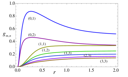
Figure 1: (Color online) Cross-correlation function between the two modes ${\small a}$ and ${\small b}$ as a function of ${\small r}$ for different parameters (m,n) and ${\small\bar{n}=0.01.}$

In order to see clearly the variation of $g_{m,n}$-parameter, we plot the graph of $g_{m,n}$ as the function of $r$ for some different ($m,n$) and $\bar{n}$ values. It is shown that $g_{m,n}$ are always larger than zero, thus there exist correlations between the two modes. This implies that the nonclassicality is enhanced by adding photon to squeezed state. For given ($m,n$) and $\bar{n}$ values, $g_{m,n}$ increases as $r$ increasing; while $g_{m,n}$ decreases as $\bar{n}$ decreasing for a given ($m,n$) value. It is interesting to notice that for single-photon-addition TMSTS, the $g_{m,n}$ parameter presents its maximum value, which implies that single-photon-addition TMSTS may possess a stronger nonclassicality than the other TMSTSs. To compare the further nonclassicality of quantum states for a different number added case, the measurments based on the volume of the negative part of the Wigner function 35 , on the nonclassical depth 36 , and on the entanglement potential 37 , Vogel’s noncalssicality criterion 38 and the Klyshko criterion 39 may be other alternative methods.

III.2 Distribution of photon number of the PA-TMSTS

In order to obtain the photon number distribution (PND) of the PA-TMSTS, we begin with evaluating the PND of TMSTS. For two-mode case described by density operator $\rho^{S}$, the PND is defined by $\mathcal{P}(m_{a},n_{b})=\left\langle m_{a},n_{b}\right|\rho^{S}\left|m_{a},n_{b}\right\rangle.$ Employing the non-normalized coherent state $\left|\alpha\right\rangle=\exp[\alpha a^{{\dagger}}]\left|0\right\rangle$ leading to $\left|n\right\rangle=\frac{1}{\sqrt{n!}}\left.\frac{d^{n}}{d\alpha^{n}}\left|\alpha\right\rangle\right|_{\alpha=0}$ $\left(\left\langle\beta\right.\left|\alpha\right\rangle=e^{\alpha\beta^{\ast}}\right)$, as well as the normal ordering form of $\rho^{S}$ in Eq.(7), the probability of finding $\left(m_{a},n_{b}\right)$ photons in the two-mode field is given by

$$\mathcal{P}(m_{a},n_{b}) = \frac{A_{1}}{m_{a}!n_{b}!}\frac{d^{2m_{a}+2n_{b}}}{d\alpha^{m_{a}}d\alpha^{\ast m_{a}}d\beta^{n_{b}}d\beta^{\ast n_{b}}}$$ (30)

$$\times\left.e^{\left(1-A_{3}\right)\left(\alpha^{\ast}\alpha+\beta^{\ast}\beta\right)+A_{2}\left(\alpha\beta+\alpha^{\ast}\beta^{\ast}\right)}\right|_{\alpha,\beta,\alpha^{\ast},\beta^{\ast}=0}$$

$$= A_{1}\left[\allowbreak\bar{n}\left(\bar{n}+1\right)\right]^{n_{b}-m_{a}}\frac{\mu\allowbreak^{m_{a}}}{\nu^{n_{a}}}P_{m_{a}}^{(n_{b}-m_{a},0)}\left(\chi\right),$$

where in the last step, we have used the new formula in Eq.(23), and

$$\nu = \left(2\bar{n}+\allowbreak 1\right)\cosh^{2}r+\bar{n}^{2},$$

$$\mu = \left(2\bar{n}+1\right)\cosh^{2}r-\left(\bar{n}+1\right)^{2},$$

$$\chi = \frac{\left(\left(2\bar{n}+1\right)\sinh 2r\right)^{2}+4\allowbreak\bar{n}^{2}\left(\bar{n}+1\right)^{2}}{\left(\left(2\bar{n}+1\right)\sinh 2r\right)^{2}-4\allowbreak\bar{n}^{2}\left(\bar{n}+1\right)^{2}}.$$ (31)

Thus the PND of TMSTS is also related to Jacobi polynomials of the parameter $\chi$. In particular, when $\bar{n}\rightarrow 0$ leading to $\chi\rightarrow 1$, corresponding to the two-mode squeezed vacuum, Eq.(30) reduces to

$$\mathcal{P}_{\bar{n}\rightarrow 0}(m_{a},n_{b})$$

$$=\lim_{\bar{n}\rightarrow 0}\frac{m_{a}!n_{b}!}{\left[\bar{n}^{2}+\left(2\bar{n}+1\right)\cosh^{2}r\right]^{m_{a}+n_{b}+1}}$$

$$\times\sum_{l=0}^{\min[m_{a},n_{a}]}\frac{\left(\allowbreak\allowbreak 2\bar{n}+1\right)^{2l}\left[\bar{n}\left(\bar{n}+1\right)\right]^{m_{a}+n_{b}-2l}\sinh^{2l}2r}{2^{2l}\left(l!\right)^{2}\left(n_{b}-l\right)!\left(m_{a}-l\right)!}$$

$$=\frac{\tanh^{2m_{a}}r}{\cosh^{2}r}\delta_{m_{a},n_{b}},$$ (32)

which is just the PND of two-mode squeezed vacuum state 23 . On the other hand, when $r\rightarrow 0$ corresponding to the case of two-mode thermal state, leading to $\chi\rightarrow-1,\nu\rightarrow\left(\bar{n}+1\right)^{2},\mu\rightarrow-\bar{n}^{2},A_{1}\rightarrow 1/\left(\bar{n}+1\right)^{2}$ and noting $P_{m_{a}}^{(n_{b}-m_{a},0)}(-1)=(-1)^{m_{a}},$ thus Eq.(30) becomes

$$\mathcal{P}_{r\rightarrow 0}(m_{a},n_{b})=\allowbreak\frac{\bar{n}^{n_{b}}}{\left(\bar{n}+1\right)^{n_{b}+1}}\frac{\bar{n}^{m_{a}}}{\left(\bar{n}+1\right)^{m_{a}+1}},$$ (33)

which is just the product of PNDs of two thermal fields, as expected.

Using the result (30) and noticing $a^{m}b^{n}\left|m_{a},n_{b}\right\rangle=\sqrt{m_{a}!n_{b}!/(m_{a}-m)!(n_{b}-n)!}\left|m_{a}-m,n_{b}-n\right\rangle$, we can directly obtain the PND $\mathcal{\bar{P}}^{SA}(m_{a},n_{b})\equiv\left\langle m_{a},n_{b}\right|\rho^{SA}\left|m_{a},n_{b}\right\rangle$ of the PA-TMSTS as

$$\mathcal{\bar{P}}^{SA}(m_{a},n_{b})$$ (34)

$$= \frac{N_{m,n}^{-1}m_{a}!n_{b}!}{(m_{a}-m)!(n_{b}-n)!}$$

$$\times\left\langle m_{a}-m,n_{b}-n\right|\rho^{S}\left|m_{a}-m,n_{b}-n\right\rangle$$

$$= \frac{N_{m,n}^{-1}m_{a}!n_{b}!}{(m_{a}-m)!(n_{b}-n)!}\mathcal{P}(m_{a}-m,n_{b}-n).$$

Eq.(34) is a Jacobi polynomial with a condition $m_{a}\geqslant m$ and $n_{b}\geqslant n$ which shows that the photon-number ($m_{a},n_{b}$) involved in PA-TMSTS are always no-less than the photon-number ($m,n$) operated on the TMSTS, and there is no photon distribution when $m_{a}<m$ and $n_{b}<n$. Here we should point out that this result (30) can be applied directly to calculate the PND of some other non-Gaussian states generated by subtracting photons from (or adding photons to) two-mode squeezed thermal states, such as $a^{m}b^{n}\rho^{S}a^{\dagger m}b^{\dagger n},$ and $a^{m}b^{{\dagger}n}\rho^{S}b^{n}a^{{\dagger}m}$.

III.3 Antibunching effect of the PA-TMSTS

Next we will discuss the antibunching for the PA-TMSTS. The criterion for the existence of antibunching in two-mode radiation is given by 40

$$R_{ab}\equiv\frac{\left\langle a^{\dagger 2}a^{2}\right\rangle+\left\langle b^{\dagger 2}b^{2}\right\rangle}{2\left\langle a^{\dagger}ab^{\dagger}b\right\rangle}-1<0.$$ (35)

In a similar way to Eq.(29) we have

$$\left\langle a^{\dagger 2}a^{2}\right\rangle = \frac{N_{m+2,n}}{N_{m,n}}-4\frac{N_{m+1,n}}{N_{m,n}}+2,$$

$$\left\langle b^{\dagger 2}b^{2}\right\rangle = \frac{N_{m,n+2}}{N_{m,n}}-4\frac{N_{m,n+1}}{N_{m,n}}+2.$$ (36)

Thus, for the state $\rho^{SA}$, substituting Eqs.(36), (28) and (24) into Eq.(35), yields

$$R_{ab} = \frac{N_{m+2,n}+N_{m,n+2}+2\left(\Omega-N_{m+1,n+1}\right)}{2\left(N_{m+1,n+1}+\Omega\right)},$$

$$\left(\Omega=N_{m,n}-N_{m+1,n}-N_{m,n+1}\right).$$

In particular, when $m=n=0$ (corresponding to the TMSTS) leading to $N_{0,0}=1,N_{0,1}=N_{1,0}=B_{1}$, and $N_{1,1}=\upsilon$, $N_{0,2}=N_{2,0}=B_{1}^{2}$, thus Eq.(III.3) becomes

$$R_{ab,m=n=0}=-\frac{\left(2\bar{n}+1\right)\left(4\cosh 2r+\left(2\bar{n}+1\right)\sinh^{2}2r\right)}{\left(2\bar{n}+1\right)\left[\left(2\bar{n}+1\right)\cosh 4r-2\cosh 2r\right]+1}.$$ (38)

From Eq.(38), it is easily seen that $R_{ab,m=n=0}<0$ for any $\bar{n}$ and non-zero $r$ values. In addition, when $m=n,$ the PA-TMSTS can always be antibunching for a small value $\bar{n}$ (see Fig.2(a)). However, for any parameter values $m,n(m\neq n)$, the case is not true. The $R_{ab}$ parameter as a function of $r$ and $m,n$ is plotted in Fig. 2. It is easy to see that, for a given $m$ the PA-TMSTS presents the antibunching effect when the squeezing parameter $r$ exceeds to a certain threshold value. For instance, when $m=0\$and $n=1$ then $R_{ab}\$may be less than zero with $r>0.1$ thereabout ($\bar{n}=0.01$). The value $R_{ab}$ parameter increases with $\bar{n}$ increasing.

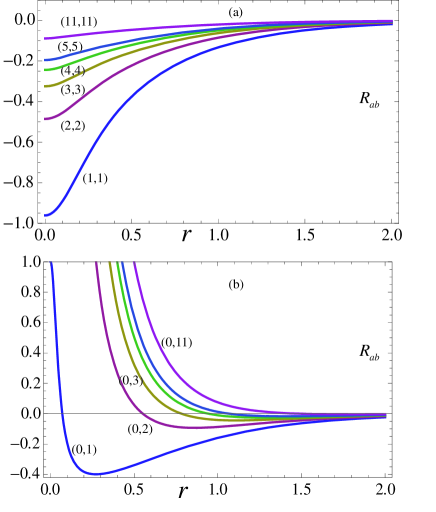
Figure 2: (Color online) ${\small R}_{ab}$ as a function of ${\small r}$ for different parameters (m,n) and ${\small\bar{n}=0.01.}$

III.4 Wigner function of PA-TMSTS

For further discussing the nonclassicality of PA-TMSTS, we examine its Wigner function (WF) whose partial negativity implies the highly nonclassical properties of quantum states. In this section, we derive the analytical expression of WF for the PA-TMSTS. The normally ordering form of the PA-TMSTS shall be used to realize our purpose.

For the two-mode case, the WF $W\left(\alpha,\beta\right)$ associated with a quantum state $\rho$ can be derived as follows 42 :

$$W\left(\alpha,\beta\right) = e^{2(\left|\alpha\right|^{2}+\left|\beta\right|^{2})}\int\frac{\mathtt{d}^{2}z_{1}\mathtt{d}^{2}z_{2}}{\pi^{4}}\left\langle-z_{1},-z_{2}\right|\rho\left|z_{1},z_{2}\right\rangle$$ (39)

$$\times\exp\left[2\left(\alpha z_{1}^{\ast}-\alpha^{\ast}z_{1}\right)+2\left(\beta z_{2}^{\ast}-\beta^{\ast}z_{2}\right)\right],$$

where $\left|z_{1},z_{2}\right\rangle=\left|z_{1}\right\rangle\left|z_{2}\right\rangle$ is the two-mode coherent state.

Substituting Eq.(17) into Eq.(39), we can finally obtain the WF of the PA-TMSTS (see Appendix C),

$$W_{m,n}\left(\alpha,\beta\right)=W_{0}\left(\alpha,\beta\right)F_{m,n}\left(\alpha,\beta\right),$$ (40)

where $W_{0}\left(\alpha,\beta\right)$ is the WF of TMSTS,

$$W_{0}\left(\alpha,\beta\right) = \frac{\pi^{-2}}{\left(2\bar{n}+1\right)^{2}}\exp\left\{-2\frac{\cosh 2r}{2\bar{n}+1}(\left|\alpha\right|^{2}+\left|\beta\right|^{2})\right.$$ (41)

$$+\allowbreak\left.2\frac{\sinh 2r}{2\bar{n}+1}\left(\beta\alpha+\alpha^{\ast}\beta^{\ast}\right)\right\},$$

and

$$F_{m,n}\left(\alpha,\beta\right) = \frac{K_{3}^{m+n}}{N_{m,n}}\sum_{l=0}^{m}\sum_{j=0}^{n}\frac{\left(m!n!\right)^{2}\left(-K_{1}/K_{3}\right)^{l+j}}{l!j!\left[\left(m-l\right)!\left(n-j\right)!\right]^{2}}$$ (42)

$$\times\left|H_{m-l,n-j}\left(\frac{R_{1}}{i\sqrt{K_{3}}},\frac{R_{3}}{i\sqrt{K_{3}}}\right)\right|^{2},$$

where we have set

$$R_{1} = 2\left(K_{1}\allowbreak\alpha-K_{3}\beta^{\ast}\right),R_{3}=2\left(K_{1}\beta-K_{3}\alpha^{\ast}\right),$$

$$K_{1} = \frac{\bar{n}+\cosh^{2}r}{2\bar{n}+1},K_{3}=\frac{\sinh r\cosh r}{2\bar{n}+1}.$$ (43)

Equation (40) is just the analytical expression of the WF for the PA-TMSTS, a real function as expected. It is obvious that the WF lost its Gaussian property in phase space due to the presence of two-variable Hermite polynomials $H_{m-l,n-j}\left(x,y\right)$.

From Eq.(42), we see that when $m=n=0$ corresponding to the TMSTS, $F_{0,0}=1,$ and $W_{m,n}\left(\alpha,\beta\right)=W_{0}\left(\alpha,\beta\right)$; whereas for the case of $m=0$ and $n\neq 0$, noticing $H_{0,n}\left(x,y\right)=y^{n}$ and $N_{0,n}=n!B_{1}^{n},$ Eq.(40) reduces to

$$W_{0,n}\left(\alpha,\beta\right)=W_{0}\left(\alpha,\beta\right)\left(-K_{1}/B_{1}\right)^{n}L_{n}(\left|R_{3}\right|^{2}/K_{1}),$$ (44)

where $L_{n}$ is the $n$-order Laguerre polynomial. Eq. (44) is just the WF of the PA-TMSTS generated by single-mode photon addition, which becomes the WF of the negative binomial state $S(r)\left|0,n\right\rangle$ with $\bar{n}=0$ [JOSAB, ??]. In particular, for the case of single photon-addition, $n=1$, it is found that

$$W_{0,1}\left(0,0\right)=-\frac{\left(\bar{n}+\cosh^{2}r\right)/\left(2\bar{n}+1\right)^{3}}{\left(\cosh^{2}r+\bar{n}\cosh 2r\right)\pi^{2}},$$ (45)

which implies that the WF of single PA-TMSTS always has its negative region at the phase space center $\alpha=\beta=0$. The maximum value of  $\left|W_{0,1}\right|$ decreases with the increasement of $\bar{n}$ and $r$ but not disappears, which can be seen clearly from Fig3,4. (a) and (b). Further, there are more visible negative region than the WF for the case of $m=n=1$. And the negative region will be absence for the latter with the increasing $\bar{n}$ value (see Fig3,4. (c) and (d)). In addition, from Figs 3 and 4, the squeezing in one of quadratures is clear, which can be seen as an evidence of nonclassicality of the state. For a given value $m$ and several different values $n$ ($\neq m$), the WF distributions are presented in Fig.5, from which it is interesting to notice that there are around $\left|m-n\right|$ wave valleys and $\left|m-n\right|+1$ wave peaks.

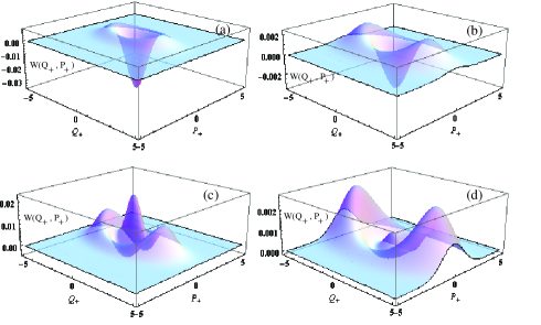
Figure 3: (Color online) The Wigner function W($\alpha,\beta$) in phase space ($Q_{+},P_{+}$) for several different parameter values $\left(m,n\right)$ and $\bar{n}$ with $r=0.3.$ (a) m=0,n=1,$\bar{n}=0.2$; (b) m=0,n=1,$\bar{n}=1$; (c) m=n=1,$\bar{n}=0.2$ and (d) m=n=1,$\bar{n}=1.$

Figure 4: (Color online) The Wigner function W($\alpha,\beta$) in phase space ($Q_{-},P_{-}$) for several different parameter values $\left(m,n\right)$ and $\bar{n}$ with $r=0.3.$ (a) m=0,n=1,$\bar{n}=0.2$; (b) m=0,n=1,$\bar{n}=1$; (c) m=n=1,$\bar{n}=0.2$ and (d) m=n=1,$\bar{n}=1.$

Figure 5: (Color online) The Wigner function W($\alpha,\beta$) in phase space ($Q_{+},P_{+}$) for several different parameter values $\left(m,n\right)$ with $\bar{n}=0.2$ and  $r=0.3.$ (a) m=0,n=2; (b) m=1,n=2; (c) m=1,n=3, and (d) m=2,n=3.

IV Entanglement properties of the PA-TMSTS

It is well known that photon subtraction/addition can be applied to improve entanglement between Gaussian states 14 ; 43 , loophole-free tests of Bell’s inequality 44 , and quantum computing 18 . In this section, we examine the entanglement properties of PA-TMSTS only with single and two photon-addition. Here, for a bipartite continuous variable state, we shall take the Shchukin-Vogel (SV) 38 criteria to describe the inseparability of PA-TMSTS.

According to the SV criteria, the sufficient condition of inseparability is

$$SV_{m,n}\equiv\left\langle a^{{\dagger}}a-\frac{1}{2}\right\rangle\left\langle b^{{\dagger}}b-\frac{1}{2}\right\rangle-\left\langle a^{{\dagger}}b^{{\dagger}}\right\rangle\left\langle ab\right\rangle<0.$$ (46)

In a similar way to derive the normalization factor Eq.(24), using Eqs.(17) and (18), we have

$$\left\langle a^{{\dagger}}b^{{\dagger}}\right\rangle=\frac{N_{m,m+1,n,n+1}}{N_{m,n}},\text{ }\left\langle ab\right\rangle=\frac{N_{m+1,m,n+1,n}}{N_{m,n}},$$ (47)

where we have set

$$N_{l,p,q,r} \equiv \left.\frac{\partial^{l+p+q+r}}{\partial\tau^{l}\partial t^{p}\partial\tau^{\prime q}\partial t^{\prime r}}e^{\left(\tau^{\prime}t^{\prime}+\tau t\right)B_{1}+\left(\tau\tau^{\prime}+tt^{\prime}\right)B_{2}}\right|_{t,\tau,t^{\prime},\tau^{\prime}=0}$$ (48)

$$= \sum_{s=0}\frac{l!r!q!p!B_{1}^{l-q+2r}B_{2}^{q-r}\left(B_{2}^{2}/B_{1}^{2}\right)^{s}\delta_{p+q,l+r}}{s!\left(q-r+s\right)!\left(r-s\right)!\left(l+r-q-s\right)!}.$$

Thus $SV$ is given by

$$SV_{m,n} = \left(\frac{N_{m+1,n}}{N_{m,n}}-\frac{3}{2}\right)\left(\frac{N_{m,n+1}}{N_{m,n}}-\frac{3}{2}\right)$$ (49)

$$-\frac{N_{m,m+1,n,n+1}}{N_{m,n}}\frac{N_{m+1,m,n+1,n}}{N_{m,n}}.$$

Next, we examine two special cases. For the case of $m=0,n=1$, using Eqs.(24) and (48), as well as noticing $N_{0,1,1,2}=N_{1,0,2,1}=2B_{1}B_{2}$, Eq.(49) becomes

$$SV_{0,1}=\left(\frac{\upsilon}{B_{1}}-\frac{3}{2}\right)\left(2B_{1}-\frac{3}{2}\right)-4B_{2}^{2}.$$ (50)

While for the case of $m=n=1$, it is shown that ($N_{1,2,1,2}=N_{2,1,2,1}=2\left(\allowbreak 2B_{1}^{2}+B_{2}^{2}\right)B_{2}$)

$$SV_{1,1}=\left(B_{1}\left(3-\frac{\omega}{\upsilon}\right)-\frac{3}{2}\right)^{2}-4\frac{\left(\allowbreak 2B_{1}^{2}+B_{2}^{2}\right)^{2}B_{2}^{2}}{\upsilon^{2}}.$$ (51)

In particular, when $\bar{n}=0$, i.e., the single PA-TMSVS, Eq.(50) is always negative for any $r>0,$ as expected (also see Fig.6 (a)). In general, it is difficult to obtain the explicit expressions of the sufficient condition of inseparability for the above cases. Here, we appeal to the number calculation shown in Fig.6. It is shown that for single PA-TMSTS with a smaller average photon number $\bar{n}$, the condition $SV_{0,1}<0$ can always be satisfied only if $r>0$; while for a larger $\bar{n}$ then the condition $SV_{0,1}<0$ is satisfied only when the squeezing parameter $r$ exceeds a certain threshold value $r_{a}$. However, it is very interesting to notice that for the photon-subtraction TMSTS, there is a threshold value $r_{c}$ for any $\bar{n}$, i.e., $r>r_{c}\equiv\frac{1}{2}\ln(2\bar{n}+1)$ 45 , which is different from the case of single PA-TMSTS. For instance, for $\bar{n}=1,$ the two threshold values are $r_{a}\approx 0.31$ and $r_{c}\approx 0.55$. This comparision may imply that the photon-addition to the TMSTS can be more effective for the entanglement enhancement than the photon-subtraction from the TMSTS. On the other hand, for the case of the PA-TMSTS with $m=n=1$ (see Fig.6 (b)), it is found that a certain threshold is needed for satisfying this condition $SV_{1,1}<0,$ which is also smaller than that of the photon-subtraction TMSTS.

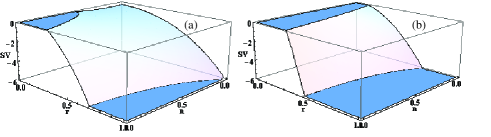
Figure 6: (Color online) The sufficient condition of inseparability as the function of ${\small r}$ and $\bar{n},$ for (a) m=0 and n=1; (b) m=n=1.

V Quantum teleportation with PA-TMSTS

As mentioned above, photon-subtraction from or photon-addition to bipartite Gaussian states can be used to improve the entanglement. In this section, we investigate the quantum teleportation with PA-TMSTS, especially for the cases $m=0,n=1$ and $m=n=1$. The role of teleportation in the CV quantum information is analyzed in the review Ref.46 .

Here, we consider the QT by using PA-TMSTS as entangled resource. Using the normal ordering form Eq.(17) and noticing the displacement operator $D_{a}\left(\alpha\right)=e^{\left|\alpha\right|^{2}/2}e^{-\alpha^{\ast}a}e^{\alpha a^{\dagger}}$, then the characteristic function (CF) of PA-TMSTS is given by (see Appendix D)

$$\chi_{E}\left(\alpha,\beta\right) = \frac{1}{N_{m,n}}e^{-(B_{1}-\frac{1}{2})(\left|\alpha\right|^{2}+\left|\beta\right|^{2})+B_{2}\left(\alpha\beta+\alpha^{\ast}\beta^{\ast}\right)}$$ (52)

$$\times\frac{\partial^{2m+2n}}{\partial\tau^{m}\partial\tau^{\prime n}\partial t^{m}\partial t^{\prime n}}e^{B_{1}\left(\tau^{\prime}t^{\prime}+t\tau\right)+B_{2}\left(t^{\prime}t+\tau^{\prime}\tau\right)}$$

$$\times e^{t\left(\alpha B_{1}-\allowbreak B_{2}\beta^{\ast}\right)+\tau\left(\beta B_{2}-B_{1}\alpha^{\ast}\right)}$$

$$\times\left.e^{\tau^{\prime}\left(\alpha B_{2}-B_{1}\beta^{\ast}\right)+t^{\prime}\left(\beta\allowbreak B_{1}-B_{2}\alpha^{\ast}\right)}\right|_{t,\tau,t^{\prime},\tau^{\prime}=0},$$

where for further calculation the differential form of $\chi_{E}$ is kept.

To quantify the performance of a QT protocol, the fidelity of QT is commonly used as a measure, $\mathcal{F=}\mathtt{tr}\left(\rho_{in}\rho_{out}\right)$, a overlap between a pure input state $\rho_{in}$ and the output (teleported, mixed) state $\rho_{out}$. For a CV system, a teleportation protocol has been given in terms of the CFs of the quantum states involved (input, source and teleported (output) states) 47 . It is shown that the CF $\chi_{out}\left(\eta\right)$ of the output state has a remarkably factorized form

$$\chi_{out}\left(\eta\right)=\chi_{in}\left(\eta\right)\chi_{E}\left(\eta^{\ast},\eta\right),$$ (53)

where $\chi_{in}\left(\eta\right)$ and $\chi_{E}\left(\eta^{\ast},\eta\right)$ are the CFs of the input state and the entangled source, respectively. Then the fidelity of QT of CVs reads 47

$$\mathcal{F=}\int\frac{d^{2}\eta}{\pi}\chi_{in}\left(\eta\right)\chi_{out}\left(-\eta\right).$$ (54)

Here, we consider the Braunstein and Kimble protocol 48 of QT for single-mode coherent-input states $\left|\gamma\right\rangle$. Note that the fidelity is independent of amplitude of the coherent state, thus for simplicity we take $\gamma=0$, then we have only to calculate the fidelity of the vacuum input state with the CF $\chi_{in}\left(\eta\right)=\exp[-\left|\eta\right|^{2}/2]$. On substituting these CFs into Eq.(54), we worked out the fidelity for teleporting a coherent state by using the PA-TMSTS as an entangled resource,

$$\mathcal{F}_{m,n}^{\bar{n}} = \frac{(m+n)!}{B_{1}-B_{2}}\frac{\left(B_{1}+B_{2}\right)^{m+n}}{2^{m+n+1}N_{m,n}}$$ (55)

$$= \frac{\left[\allowbreak\left(2\bar{n}+1\right)e^{2r}+\allowbreak 1\right]^{m+n}}{\allowbreak\left(2\bar{n}+1\right)e^{-2r}+1}\frac{(m+n)!}{2^{2m+2n}N_{m,n}}.$$

It can be seen that the fidelity is not only dependent on the parameter $r$, the average photon-number $\bar{n}$, but also on the photon number $\left(m,n\right)$ added to each mode of the TMSTS. In particular, when $m=n=0,$ Eq.(55) just reduces to

$$\mathcal{F}_{0,0}^{\bar{n}}=\frac{1}{\allowbreak\left(2\bar{n}+1\right)e^{-2r}+1},$$ (56)

which leads to the condition $r>\frac{1}{2}\ln\left(2\bar{n}+1\right)$ for satisfying the effective QT with $\mathcal{F}>\frac{1}{2}$ which is the classical limit. In addition, for the case of $\bar{n}=0$, i.e., the photon-added TMSVS, Eq.(55) becomes

$$\mathcal{F}_{m,n}^{0}=\frac{\left(\allowbreak e^{2r}+\allowbreak 1\right)^{n+m}}{\allowbreak e^{-2r}+1}\frac{(m+n)!}{2^{2m+2n}N_{m,n}}.$$ (57)

Further,  when $\left(m,n\right)=\left(0,0\right),\left(1,1\right)$ and $\left(0,1\right)$, Eq.(56) just reduce, respectively, to

$$\mathcal{F}_{0,0}^{0} \mathcal{=} (1+\tanh r)/2,$$

$$\mathcal{F}_{1,1}^{0} = \frac{(1+\tanh r)^{3}}{4(1+\tanh^{2}r)},$$

$$\mathcal{F}_{0,1}^{0} = \frac{1+\tanh r}{4\left(1-\tanh r\right)}\text{sech}^{2}r.$$ (58)

The two expressions $\mathcal{F}_{0,0}^{0}$ and $\mathcal{F}_{1,1}^{0}$ are agreement with Eqs.(15) and (17) in Ref. 49 .

In Fig. 7, for some given $\left(m,n\right)$ values, the fidelity of teleporting the coherent state is shown as a function of $r$ by using the PA-TMSTS as the entangled resource. It is shown that the fidelity with this resource is smaller than that with TMSTS, although the PA-TMSTS posesses larger entanglement 49 . In addition, for the symmetrical case $m=n$, when the squeezing parameter $r$ exceeds a certain threshold value, the fidelity increases with a increasing $m$ (see Fig.7(c)); while for non-symmetric case $m\neq n$, the fidelity decreases with increasing $n\$(see Fig.7(b)). For the former, the threshold value $r$ decreases with increasing $m\left(=n\right)$; the case is not true for the latter. This indicate that the symmetrical PA-TMSTS may be more effective for QT than the non-symmetric case.

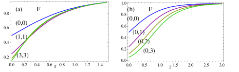
Figure 7: (Color online) The fidelity as the function of ${\small r}$ for several different (m,n) values and $\bar{n}{\small=0.01}.$

VI Conclusions

In this paper, we introduce the PA-TMSTS and investigate its entanglement and nonclassicality. By using the coherent state representation of thermal state, the normally and antinormally ordering forms of the TMSTS are obtained. Based on this, the normalization factor of the PA-TMSTS is derived, which is related to the Jacobi polynomials of the squeezing parameter $r$ and average photon number $\bar{n}$ of the thermal state. Then we discuss the nonclassical properties by using cross-correlation function, distribution of photon number, antibunching effect and the negativity of its WF. It is found that the WF lost its Gaussian property in phase space due to the presence of two-variable Hermite polynomials and the WF of single PA-TMSTS always has its negative region at the center of phase space. Further, there are more visible negative region than the WF for the case of $m=n=1$. And the negative region will be absence for the latter with the increasing $\bar{n}$ value. The entanglement properties of the PA-TMSTS by Shchukin-Vogel criteria and the quantum teleportation. It is shown that the photon-addtion to the TMSTS can be more effective for the entanglement enhancement than the photon-subtraction from the TMSTS; And using the PA-TMSTS as an entangled resource, the fidelity for teleporting a coherent state is not only dependent on the parameter $r$, the average photon-number $\bar{n}$, but also on the photon number $\left(m,n\right)$ added to each mode of the TMSTS. From this point, the symmetrical PA-TMSTS may be more effective for quantum teleportation than the non-symmetric case.

Acknowledgments: This work was supported by the NSFC (Grant No. 60978009), the Major Research Plan of the NSFC (Grant No. 91121023), and the “973” Project (Grant No. 2011CBA00200), and the Natural Science Foundation of Jiangxi Province of China (No. 2010GQW0027) as well as the Sponsored Program for Cultivating Youths of Outstanding Ability in Jiangxi Normal University.

Appendix A: Derivation of Eq.(18)

According to the normalization condition, $\mathtt{tr}\rho^{SA}=1,$ we have

$$N_{m,n} =A_{1}\mathtt{tr}\left[\colon a^{\dagger m}b^{\dagger n}e^{A_{2}\left(a^{\dagger}b^{\dagger}+ab\right)-A_{3}\left(a^{\dagger}a+b^{\dagger}b\right)}a^{m}b^{n}\colon\right]$$

$$=\frac{A_{1}\partial^{2m+2n}}{\partial\tau^{m}\partial t^{m}\partial\tau^{\prime n}\partial t^{\prime n}}\mathtt{tr}\left[\colon e^{A_{2}\left(a^{\dagger}b^{\dagger}+ab\right)-A_{3}\left(a^{\dagger}a+b^{\dagger}b\right)+\tau a^{\dagger}+ta+\tau^{\prime}b^{\dagger}+t^{\prime}b}\colon\right].$$ (A1)

Using the completeness relation of coherent state $\int d^{2}\alpha d^{2}\beta\left|\alpha,\beta\right\rangle\left\langle\alpha,\beta\right|/\pi^{2}=1$ and Eq.(9), Eq.(A1)

$$N_{m,n} =A_{1}\int\frac{d^{2}\alpha d^{2}\beta}{\pi^{2}}\left|\alpha\right|^{2m}\left|\beta\right|^{2n}e^{A_{2}\left(\alpha^{\ast}\beta^{\ast}+\alpha\beta\right)-A_{3}(\left|\alpha\right|^{2}+\left|\beta\right|^{2})}$$

$$=\frac{A_{1}\partial^{2m+2n}}{\partial\tau^{m}\partial t^{m}\partial\tau^{\prime n}\partial t^{\prime n}}\int\frac{d^{2}\alpha d^{2}\beta}{\pi^{2}}\exp\left[-A_{3}(\left|\alpha\right|^{2}+\left|\beta\right|^{2})\right.$$

$$\left.+\left(A_{2}\beta+\tau\right)\alpha+\left(A_{2}\beta^{\ast}+t\right)\alpha^{\ast}+\tau^{\prime}\beta+t^{\prime}\beta^{\ast}\right]_{t,\tau,t^{\prime},\tau^{\prime}=0}.$$ (A2)

Using Eq.(9), (A2) becomes

$$N_{m,n} =\frac{A_{1}\partial^{2m+2n}}{\partial\tau^{m}\partial t^{m}\partial\tau^{\prime n}\partial t^{\prime n}}\frac{1}{A_{3}}\int\frac{d^{2}\beta}{\pi}\exp\left[-\frac{A_{3}^{2}-A_{2}^{2}}{A_{3}}\left|\beta\right|^{2}\right.$$

$$+\left.\left(\frac{A_{2}t}{A_{3}}+\tau^{\prime}\right)\beta+\left(\frac{A_{2}\tau}{A_{3}}+t^{\prime}\right)\beta^{\ast}+\frac{\tau t}{A_{3}}\right]_{t,\tau,t^{\prime},\tau^{\prime}=0}$$

$$=\text{LHS of Eq.(\ref{t18})},$$ (A3)

where we have used $A_{1}/(A_{3}^{2}-A_{2}^{2})=1$ and $B_{2}=A_{2}\allowbreak/(A_{3}^{2}-A_{2}^{2})=\left(2\bar{n}+1\right)\sinh r\cosh r$ as well as $B_{1}=A_{3}/(A_{3}^{2}-A_{2}^{2})$.

Appendix B: New expression of generating function for Jacobi polynomials

In this appendix, we shall prove Eq.(23). Rewriting

$$H\equiv\left.\frac{\partial^{2m+2n}}{\partial\tau^{m}\partial t^{m}\partial\tau^{\prime n}\partial t^{\prime n}}e^{A\left(\tau^{\prime}t^{\prime}+\tau t\right)+B\left(\tau\tau^{\prime}+t^{\prime}t\right)}\right|_{t,\tau,t^{\prime},\tau^{\prime}=0}.$$ (B1)

Expanding the exponential items, we see

$$H =\sum_{l,j,k,s=0}^{\infty}\frac{A^{l+j}B^{s+k}}{l!j!k!s!}\left.\frac{\partial^{2m+2n}}{\partial\tau^{m}\partial t^{m}\partial\tau^{\prime n}\partial t^{\prime n}}\tau^{k+j}t^{j+s}\tau^{\prime l+k}t^{\prime l+s}\right|_{t,\tau,t^{\prime},\tau^{\prime}=0}$$

$$=\sum_{s=0}^{\min\left[m,n\right]}\frac{\left(m!n!\right)^{2}A^{n+m}}{s!s!\left(n-s\right)!\left(m-s\right)!}\left(\frac{B^{2}}{A^{2}}\right)^{s}.$$ (B2)

Comparing Eq.(B2) with the standard expression of Jacobi polynomials,

$$P_{m}^{(\alpha,\beta)}(x)=\left(\frac{x-1}{2}\right)^{m}\sum_{k=0}^{m}\left(\begin{array}[]{c}m+\alpha\\ k\end{array}\right)\left(\begin{array}[]{c}m+\beta\\ m-k\end{array}\right)\left(\frac{x+1}{x-1}\right)^{k},$$ (B3)

we can find that taking $m\leqslant n$ and $y=\left(B^{2}+A^{2}\right)/\left(B^{2}-A^{2}\right)$,

$$H =\sum_{s=0}^{m}\frac{\left(m!n!\right)^{2}A^{n+m}}{s!s!\left(n-s\right)!\left(m-s\right)!}\left(\frac{B^{2}}{A^{2}}\right)^{s}$$

$$=m!n!\left(\frac{y-1}{2}\right)^{-m}A^{m+n}\left\{\left(\frac{y-1}{2}\right)^{m}\right.$$

$$\times\left.\sum_{k=0}^{\min[m,n]}\frac{m!n!}{k!k!\left(n-k\right)!\left(m-k\right)!}\left(\frac{y+1}{y-1}\right)^{k}\right\}$$

$$=m!n!A^{n-m}\left(B^{2}-A^{2}\right)^{m}P_{m}^{(n-m,0)}\left(y\right).$$ (B4)

In a similar way, for $n\leqslant m$, we also have

$$H=m!n!A^{m-n}\left(B^{2}-A^{2}\right)^{n}P_{n}^{(m-n,0)}\left(y\right).$$ (B5)

Thus we finish the proof of Eq.(23).

In addition, when $m=n$, Eq.(23) becomes

$$\left.\frac{\partial^{4m}}{\partial\tau^{m}\partial t^{m}\partial\tau^{\prime m}\partial t^{\prime m}}e^{A\left(\tau^{\prime}t^{\prime}+\tau t\right)+B\left(\tau\tau^{\prime}+t^{\prime}t\right)}\right|_{t,\tau,t^{\prime},\tau^{\prime}=0}$$

$$=\left.\frac{\partial^{4m}}{\partial\tau^{m}\partial t^{m}\partial\tau^{\prime m}\partial t^{\prime m}}e^{\left(At^{\prime}+B\tau\right)\tau^{\prime}+\left(A\tau+Bt^{\prime}\right)t}\right|_{t,\tau,t^{\prime},\tau^{\prime}=0}$$

$$=\left.\frac{\partial^{4m}}{\partial\tau^{m}\partial t^{m}}\left[\left(At+B\tau\right)\left(A\tau+Bt\right)\right]^{m}\right|_{\tau,t^{\prime}=0}$$

$$=\left(m!\right)^{2}\left(B^{2}-A^{2}\right)^{m}P_{m}\left(\frac{B^{2}+A^{2}}{B^{2}-A^{2}}\right),$$ (B6)

where $P_{m}\left(x\right)$ is the $m$th Legendre polynomials. Eq.(B6) is just a new formula for the generating function of Legendre polynomials $P_{m}(x)$, which is different from the new form found in Ref.50 . In fact, one can check Eq. (B6) by expanding directly the whole exponential items and comparing with the standard expression of Legendre polynomials.

Appendix C: Derivation of Eq.(40)

Substituting Eq.(17) into Eq.(39) and usiing Eq.(9), we have

$$W\left(\alpha,\beta\right) =A_{1}N_{m,n}^{-1}e^{2(\left|\alpha\right|^{2}+\left|\beta\right|^{2})}\frac{\partial^{2m+2n}}{\partial\tau^{m}\partial t^{m}\partial\tau^{\prime n}\partial t^{\prime n}}\int\frac{d^{2}z_{1}d^{2}z_{2}}{\pi^{4}}$$

$$\times\exp\left\{-\left(2-A_{3}\right)\left|z_{1}\right|^{2}-\left(2-A_{3}\right)\left|z_{2}\right|^{2}\right.$$

$$+\left(t-2\alpha^{\ast}+A_{2}z_{2}\right)z_{1}+\left(2\alpha+\tau+A_{2}z_{2}^{\ast}\right)z_{1}^{\ast}$$

$$\left.\left.+2\left(\beta z_{2}^{\ast}-\beta^{\ast}z_{2}\right)+\tau^{\prime}z_{2}^{\ast}+t^{\prime}z_{2}\right\}\right|_{t,t^{\prime},\tau,\tau^{\prime}=0}$$

$$=W_{0}\left(\alpha,\beta\right)F_{m,n}\left(\alpha,\beta\right),$$ (C1)

where $W_{0}\left(\alpha,\beta\right)$ is defined in Eq.(41), and

$$F_{m,n}\left(\alpha,\beta\right) =\frac{\left(-1\right)^{m+n}}{N_{m,n}}\frac{\partial^{2m+2n}}{\partial\tau^{m}\partial t^{m}\partial\tau^{\prime n}\partial t^{\prime n}}$$

$$\times e^{R_{1}t+R_{2}\tau+R_{3}t^{\prime}+R_{4}\tau^{\prime}}$$

$$\times\left.e^{K_{1}\left(\tau t+\tau^{\prime}t^{\prime}\right)+K_{3}\left(\tau\tau^{\prime}+tt^{\prime}\right)}\right|_{t,t^{\prime},\tau,\tau^{\prime}=0},$$ (C2)

and

$$R_{1} =2\left(K_{1}\allowbreak\alpha-K_{3}\beta^{\ast}\right)=-R_{2}^{\ast},$$

$$R_{3} =2\left(K_{1}\beta-K_{3}\alpha^{\ast}\right)=-R_{4}^{\ast},$$ (C3)

as well as

$$K_{1}=\frac{\bar{n}+\cosh^{2}r}{2\bar{n}+1},K_{3}=\frac{\sinh r\cosh r}{2n+1}.$$ (C4)

Expanding the partial exponential items in Eq.(C2), then Eq.(C2) becomes

$$F_{m,n}\left(\alpha,\beta\right)$$

$$=\frac{\left(-1\right)^{m+n}}{N_{m,n}}\frac{\partial^{2m+2n}}{\partial\tau^{m}\partial t^{m}\partial\tau^{\prime n}\partial t^{\prime n}}\sum_{l,j=0}^{\infty}\frac{K_{1}^{l+j}}{l!j!}$$

$$\times\left.\left(\tau t\right)^{l}\left(\tau^{\prime}t^{\prime}\right)^{j}e^{R_{1}t+R_{3}t^{\prime}-R_{1}^{\ast}\tau-R_{3}^{\ast}\tau^{\prime}+K_{3}\left(\tau\tau^{\prime}+tt^{\prime}\right)}\right|_{t,t^{\prime},\tau,\tau^{\prime}=0}$$

$$=\frac{\left(-1\right)^{m+n}}{N_{m,n}}\sum_{l,j=0}^{\infty}\frac{K_{1}^{l+j}}{l!j!}\frac{\partial^{2l+2j}}{\partial\left(-R_{1}^{\ast}\right)^{l}\partial R_{1}^{l}\partial\left(-R_{3}^{\ast}\right)^{j}\partial R_{3}^{j}}$$

$$\left.\frac{\partial^{2m+2n}}{\partial\tau^{m}\partial t^{m}\partial\tau^{\prime n}\partial t^{\prime n}}e^{R_{1}t+R_{3}t^{\prime}-R_{1}^{\ast}\tau-R_{3}^{\ast}\tau^{\prime}+K_{3}\left(\tau\tau^{\prime}+tt^{\prime}\right)}\right|_{t,t^{\prime},\tau,\tau^{\prime}=0}.$$ (C5)

Further using the generating function of two-variable Hermite polynomials,

$$\left.\frac{\partial^{m}}{\partial\tau^{m}}\frac{\partial^{n}}{\partial\upsilon^{n}}e^{-A\tau\upsilon+B\tau+C\upsilon}\right|_{\tau=\upsilon=0}$$

$$=(\sqrt{A})^{m+n}H_{m,n}\left(\frac{B}{\sqrt{A}},\frac{C}{\sqrt{A}}\right),$$ (C6)

Eq.(C5) can be put into the following form

$$F_{m,n}\left(\alpha,\beta\right) =\frac{K_{3}^{m+n}}{N_{m,n}}\sum_{l,j=0}^{\infty}\frac{K_{1}^{l+j}}{l!j!}\frac{\partial^{2l+2j}}{\partial\left(-R_{1}^{\ast}\right)^{l}\partial R_{1}^{l}\partial\left(-R_{3}^{\ast}\right)^{j}\partial R_{3}^{j}}$$

$$\times H_{m,n}\left(\frac{R_{1}}{\sqrt{-K_{3}}},\frac{R_{3}}{\sqrt{-K_{3}}}\right)$$

$$\times H_{m,n}\left(\frac{-R_{1}^{\ast}}{\sqrt{-K_{3}}},\frac{-R_{3}^{\ast}}{\sqrt{-K_{3}}}\right).$$ (C7)

Using the relation

$$\frac{\partial^{l+k}}{\partial x^{l}\partial y^{k}}H_{m,n}\left(x,y\right)=\frac{m!n!}{\left(m-l\right)!\left(n-k\right)!}H_{m-l,n-k}\left(x,y\right),$$ (C8)

thus we can obtain Eq.(42).

Appendix D: Derivation of Eq.(52)

Using the displacement operator $D_{a}\left(\alpha\right)=e^{\left|\alpha\right|^{2}/2}e^{-\alpha^{\ast}a}e^{\alpha a^{\dagger}}$ and $D_{b}\left(\beta\right)=e^{\left|\beta\right|^{2}/2}e^{-\beta^{\ast}b}e^{\beta b^{\dagger}}$ as well as the normally ordering form of PA-TMSTS (17), the CF of PA-TMSTS is given by

$$\chi_{E}\left(\alpha,\beta\right)\left.=\right.\mathtt{tr}\left[D_{a}\left(\alpha\right)D_{b}\left(\beta\right)\rho^{SA}\right]$$

$$=\frac{A_{1}e^{(\left|\beta\right|^{2}+\left|\alpha\right|^{2})/2}}{N_{m,n}}\frac{\partial^{2m+2n}}{\partial\alpha^{m}\partial\beta^{n}\partial\left(-\alpha^{\ast}\right)^{m}\partial\left(-\beta^{\ast}\right)^{n}}$$

$$\times\mathtt{tr}\left[\colon e^{\alpha a^{\dagger}+\beta b^{\dagger}-\alpha^{\ast}a-\beta^{\ast}b+A_{2}\left(a^{\dagger}b^{\dagger}+ab\right)-A_{3}\left(a^{\dagger}a+b^{\dagger}b\right)}\colon\right].$$ (D1)

In a similar way to derive Eq.(18), using Eqs.(A1) and (18), one can directly obtain

$$\chi_{E}\left(\alpha,\beta\right) =\frac{e^{(\left|\beta\right|^{2}+\left|\alpha\right|^{2})/2}}{N_{m,n}}\frac{\partial^{2m+2n}}{\partial\alpha^{m}\partial\beta^{n}\partial\left(-\alpha^{\ast}\right)^{m}\partial\left(-\beta^{\ast}\right)^{n}}$$

$$\times e^{B_{1}\left(\alpha\left(-\alpha^{\ast}\right)+\beta\left(-\beta^{\ast}\right)\right)+B_{2}\left(\alpha\beta+\left(-\alpha^{\ast}\right)\left(-\beta^{\ast}\right)\right)}.$$ (D2)

Taking the following transformations

$$\alpha \rightarrow\alpha+\tau,-\alpha^{\ast}\rightarrow t-\alpha^{\ast},$$

$$\beta \rightarrow\beta+\tau^{\prime},-\beta^{\ast}\rightarrow t^{\prime}-\beta^{\ast},$$ (D3)

which leads to

$$e^{B_{1}\left(\alpha\left(-\alpha^{\ast}\right)+\beta\left(-\beta^{\ast}\right)\right)+B_{2}\left(\alpha\beta+\left(-\alpha^{\ast}\right)\left(-\beta^{\ast}\right)\right)}$$

$$\rightarrow\exp\left[-B_{1}(\left|\alpha\right|^{2}+\left|\beta\right|^{2})+B_{2}\left(\alpha\beta+\alpha^{\ast}\beta^{\ast}\right)\right]$$

$$\times\exp\left[B_{1}\left(\tau^{\prime}t^{\prime}+t\tau\right)+B_{2}\left(t^{\prime}t+\tau^{\prime}\tau\right)\right]$$

$$\times\exp\left[t\left(\alpha B_{1}-\allowbreak B_{2}\beta^{\ast}\right)+\tau\left(\beta B_{2}-B_{1}\alpha^{\ast}\right)\right]$$

$$\times\exp\left[\tau^{\prime}\left(\alpha B_{2}-B_{1}\beta^{\ast}\right)+t^{\prime}\left(\beta\allowbreak B_{1}-B_{2}\alpha^{\ast}\right)\right],$$ (D4)

thus Eq.(D2) becomes Eq.(52).

References

- (1) D. Bouwmeester, A. Ekert and A. Zeilinger, The Physics of Quantum Information (Springer-Verlag, Berlin, 2000).
- (2) J. Eisert, S. Scheel, and M. B. Plenio, Phys. Rev. Lett. 89, 137903 (2002).
- (3) G. Giedke and J. I. Cirac, Phys. Rev. A. 66, 032316 (2002).
- (4) J. Fiurasek, Phys. Rev. Lett. 89, 137904 (2002).
- (5) T. Opatrný, G. Kurizki, and D.-G. Welsch, Phys. Rev. A 61, 032302 (2000).
- (6) A. Zavatta, S. Viciani, and M. Bellini, Science 306, 660 (2004).
- (7) A. Zavatta, S. Viciani, and M. Bellini, Phys. Rev. A 72, 023820 (2005).
- (8) H. Nha and H. J. Carmichael, Phys. Rev. Lett. 93, 020401 (2004).
- (9) J. Wenger, R. Tualle-Brouri, and P. Grangier, Phys. Rev. Lett. 92, 153601 (2004).
- (10) M. S. Kim, J. Phys. B 41, 133001 (2008).
- (11) L. Y. Hu and H. Y. Fan, J. Opt. Soc. Am. B 25, 1955 (2008).
- (12) V. Parigi, A. Zavatta, M. S. Kim, and M. Bellini, Science 317, 1890 (2007).
- (13) S. Olivares, M. G. A. Paris, and R. Bonifacio, Phys. Rev. A 67, 032314 (2003).
- (14) A. Kitagawa, M. Takeoka, M. Sasaki, and A. Chefles, Phys. Rev. A 73, 042310 (2006).
- (15) A. Ourjoumtsev, A. Dantan, R. Tualle-Brouri, and P. Grangier, Phys. Rev. Lett. 98, 030502 (2007).
- (16) A. Ourjoumtsev, R. Tualle-Brouri, and P. Grangier, Phys. Rev. Lett. 96, 213601 (2006).
- (17) L. Y. Hu, X. X. Xu and H. Y. Fan, J. Opt. Soc. Am. B 27, 286 (2010).
- (18) P. T. Cochrane, T. C. Ralph, and G. J. Milburn, Phys. Rev. A 65, 062306 (2002).
- (19) S. D. Bartlett and B. C. Sanders, Phys. Rev. A 65, 042304 (2002).
- (20) M. Sasaki and S. Suzuki, Phys. Rev. A 73, 043807 (2006).
- (21) C. Invernizzi, S. Olivares, M. G. A. Paris, and K. Banaszek, Phys. Rev. A 72, 042105 (2005).
- (22) S. Y. Lee, S. W. Ji, H. J. Kim, and H. Nha, Phys. Rev. A 84, 012302 (2011).
- (23) L. Y. Hu, and Z. M. Zhang, J. Opt. Soc. Am. B 29, (2012) to be published. or arXiv:1110.6587[quannt-ph]
- (24) G. S. Agarwal and K. Tara, Phys. Rev. A 43, 492 (1991); Phys. Rev. A 46, 485 (1992).
- (25) S. M. Barnett and P. M. Radmore, Methods in Theoretical Quantum Optics (Clarendon Press, 1997).
- (26) M. O. Scully and M. S. Zubairy, Quantum Optics (Cambridge University Press, 1998).
- (27) V. V. Dodonov, J. Opt. B 4, R1 (2002).
- (28) H Y Fan, H. L. Lu and Y. Fan, Ann. Phys. 321, 480 (2006).
- (29) FanHong-Yi, H. R. Zaidi, and J. R. Klauder, Phys. Rev. D 35, 1831 (1987).
- (30) R. R. Puri, Mathematical Methods of Quantum Optics (Springer-Verlag, 2001), Appendix A.
- (31) H. Y. Fan, L.Y. Hu, Opt. Lett. 33, 443 (2008).
- (32) P. Marian, Phys. Rev. A 45, 2044 (1992).
- (33) P. Marian, T. A. Marian and H. Scutaru, J. Phys. A: Math. Gen. 34, 6969 (2001).
- (34) Z. X. Zhang and H. Y. Fan, Phys. Lett. A 174, 206 (1993).
- (35) W. M. Zhang, D. F. Feng, and R. Gilmore, Rev. Mod. Phys. 62, 867 (1990).
- (36) M. G. Benedict and A. Czirjak, Phys. Rev. A 60, 4034 (1999).
- (37) C. T. Lee, Phys. Rev. A 44, R2775 (1991).
- (38) J. K. Asboth, J. Calsamiglia, and H. Ritsch, Phys. Rev. Lett. 94, 173602 (2005).
- (39) E. Shchukin, W. Vogel, Phys. Rev. Lett. 95, 230502 (2005).
- (40) D. N. Klyshko, Phys. Lett. A 213, 7 (1996).
- (41) C. T. Lee, Phys. Rev. A 41, 1569 (1990).
- (42) E. P. Wigner, Phys. Rev. 40, 749 (1932).
- (43) D. E. Browne, J. Eisert, S. Scheel, and M. B. Plenio, Phys. Rev.A 67, 062320 (2003).
- (44) R. García-Patrón, J. Fiurášek, N. J. Cerf, J. Wenger, R. Tualle-Brouri, and P. Grangier, Phys. Rev. Lett. 93, 130409 (2004).
- (45) X. Y. Chen, Phys. Lett. A 372, 2976 (2008).
- (46) S. L Braunstein and P. van Loock, Rev. Mod. Phys. 77, 513 (2005).
- (47) P. Marian and T. A. Marian, Phys. Rev. A 74, 042306 (2006).
- (48) S. L. Braunstein and H. J. Kimble, Phys. Rev. Lett. 80, 869 (1998).
- (49) Y. Yang and F. L. Li, Phys. Rev. A 80, 022315 (2009).
- (50) L. Y. Hu, X. X. Xu, Z. S. Wang, and X. F. Xu, Phys. Rev. A 82, 043842 (2010).