Fast Shape Estimation for Galaxies and Stars

Abstract

Model fitting is frequently used to determine the shape of galaxies and the point spread function, for examples, in weak lensing analyses or morphology studies aiming at probing the evolution of galaxies. However, the number of parameters in the model, as well as the number of objects, are often so large as to limit the use of model fitting for future large surveys. In this article, we propose a set of algorithms to speed up the fitting process. Our approach is divided into three distinctive steps: centroiding, ellipticity measurement, and profile fitting. We demonstrate that we can derive the position and ellipticity of an object analytically in the first two steps and thus leave only a small number of parameters to be derived through model fitting. The position, ellipticity, and shape parameters can then used in constructing orthonomal basis functions such as sérsiclets for better galaxy image reconstruction. We assess the efficiency and accuracy of the algorithms with simulated images. We have not taken into account the deconvolution of the point spread function, which most weak lensing analyses do.

1 Introduction

Quantifying shapes of galaxies and stars has long been one of the key tasks in astronomical image analyses. The shape of an astronomical object is one of the a few direct observables. A lot of useful information can be inferred from the shapes of galaxies and stars. For example, galaxy mophology provides important knowledge on the formation and evolution of galaxies (Kennicutt, 1998; Van de Wel et al., 2010). As one of the most promising tools to probe dark energy and dark matter in the universe, weak gravitational lensing relies on precision measurements of the ellipticities of the background galaxies and the point spread function (PSF).

The signal in weak lensing, however, is often very weak and noisy, due to the large intrinsic dispersion in the shapes of background galaxies. For ground-based observations, the shapes of galaxies are further distorted by atmospheric turbulence and optical distortions, which can be described by the PSF, and quantified using shapes of stars. The first weak lensing algorithm was proposed by Kaiser et al. (1995) (hereafter KSB) and improved by Luppino & Kaiser (1997) and Hoekstra et al. (1998). Since then, a variety of algorithms were proposed and a series of data analysis challenges have been carried out to improve the precision and reduce systematic biases (Heymans et al., 2006; Massey et al., 2007; Bridle et al., 2010, Kitching et al., 2010 and the references therein). However, none of the algorithms satisfies the requirements of future surveys such as the Dark Energy Survey (DES), the Canada-France-Hawaii-Telescope Legacy Survey (CFHTLS), and the Large Synoptic Survey Telescope (LSST). Given the enormous amount of galaxies to be covered by these surveys, one limiting factor of the existing algorithms is the accuracy and efficiency with which the shapes and galaxies and stars are measured.

One of the existing powerful tools that has been studied in great detail is the decompostion of images using basis functions, such as the Gaussian-Laguerre expansion (Bernstein & Jarvis, 2002), or Shapelets (Refregier, 2003; Refregier & Bacon, 2003; Massey & Refregier, 2005) or sérscilets (Ngan et al., 2009; Andrae et al., 2011). However, there are limitations to these methods, because that the zeroth order image is often a poor match to real galaxy profiles. While theoretically any intensity profile can be written as a weighted sum of any complete set of basis functions, in reality, the more the zeroth order resembles the real profile, the fewer basis functions are needed in the decompostion(Massey & Refregier, 2005; Bosch, 2010). As a first step, it is necessary to accurately and efficiently quantify the observed shape of galaxies based on noisy images, which can then be used as input in the construction of the basis functions.

In this article, we present a set of efficient algorithms specifically for the task of parameter estimations for observed galaxies, including center position, ellipticity, and shape parameters such as size and steepness. We then run numerical tests to demonstrate the effectiveness of these algorithms, and how the basis functions could help further improve the image reconstrcution. Our algorithms, developed with their weak lensing applications in mind, could also be used for others purposes such as to measure the approximate morphological parameters for large population of galaxies(e.g.,Gadotti, 2009; Wang et al., 2012). We leave PSF deconvolution to later work.

Usually, no less than six parameters are needed to model the light distribution of an object, including the centroid position $(x,y)$, the ellipticity $(g_{1},g_{2})$, the normalization $I_{0}$, and the profile parameter(s). High-dimensional parameter search is very time consuming, especially when the number of objects is large, and tends to be trapped at local minima. Instead of brute-force fitting, we propose to derive the centroid position, ellipticity, and normalization of a light distribution numerically and thus reduce the number of parameters that need to be determined through fitting. Similar effort has been previously undertaken. Miller et al. (2007) and Kitching et al. (2008) proposed a fast-fitting algorithm in Fourier space, which also takes into account the effects of PSF. Here, we will only focus on how to reproduce the observed images.

Once the observed shape of galaxies (and stars for PSF determination) is described by smooth model(s), one may proceed to use the invariants equation to arrive at the intrinsic shape of galaxies (Flusser & Suk, 1998; Melchior et al., 2011), or to do the PSF deconvolution using basis function transformations (Massey & Refregier, 2005; Melchior et al., 2009; Bosch, 2010). In practice, the simple models used to describe the light profile of stars and galaxies often lead biases in the measurements (Voigt & Bridle, 2010; Melchior et al., 2010). The situation can be improved by adopting more sophisticated spatial models or a set of basis functions. Our algorithms will be useful in providing input to the construction of basis functions (Li & Cui, 2012).

This article is organised as follows. We describe the algorithms for position and ellipticity determination in Sections 2 and 3, and numerical tests in Section 4. We conclude by discussing the limitation and prospects of our algorithm in Section 5.

2 Centroiding

For simplicity, we assume a Gaussian intensity profile and choose the origin of the coordinate system to be at the estimated center of the profile. With the actual center at ($\Delta x,\Delta y$), the intensity profile is given by

$$I(x,y)=I_{0}e^{-\frac{(x-\Delta x)^{2}+(y-\Delta y)^{2}}{2\sigma^{2}}}+\epsilon,$$ (1)

where $\epsilon$ is the noise term. Now, with a Gaussian weight function, we define

$$N =\int_{-\infty}^{\infty}I(x,y)e^{-\frac{x^{2}+y^{2}}{2\sigma_{w}^{2}}}dxdy,$$ (2)

$$<x> =\int_{-\infty}^{\infty}I(x,y)e^{-\frac{x^{2}+y^{2}}{2\sigma_{w}^{2}}}xdxdy,$$ (3)

$$<y> =\int_{-\infty}^{\infty}I(x,y)e^{-\frac{x^{2}+y^{2}}{2\sigma_{w}^{2}}}ydxdy.$$ (4)

Neglecting the noise terms, we have

$$\frac{<x>}{N} =k\Delta x,$$ (5)

$$\frac{<y>}{N} =k\Delta y,$$ (6)

where $k=\sigma_{w}^{2}/(\sigma^{2}+\sigma_{w}^{2})$.

When the intensity profile has the same shape as the weight function, $\sigma=\sigma_{w}$, we have $k=0.5$. If the former is extremely compact (i.e., $\sigma\approx 0$), we have $k=1$. In general, the value of $k$ is determined iteratively. For a true coefficient $0.5<k_{true}<1$, the choice of $k=0.75$ gives $|\Delta_{i+1}|<\frac{1}{3}|\Delta_{i}|$, where $\Delta_{i}$ is the distance between the centers of the intensity profile and the weight function in the $i$th iteration. So, the calculation converges very quickly. In typical cases, convergence is achieved in less than five iterations, and the result can be further improved using an elliptical weight function with ellipticity obtained using the algorithm described in the next section.

3 Ellipticity Measurement

Our approach is based on the KSB algorithm for shear measurement (Kaiser et al., 1995, hereafter KSB95; Luppino & Kaiser, 1997; Hoekstra et al., 1998). Because our goal here is only to estimate the ellipticity of an object, there is no convolution or deconvolution involved. This means that we are only concerned with shear polarizability $P^{SH}$.

The KSB algorithm is perturbative in nature and is applicable only when the ellipticity is small. To adapt it for general ellipticity measurement, we have adopted an iterative approach. At each step, we evaluate

$$\Delta g=g-g_{w},$$ (7)

where $g$ and $g_{w}$ are the ellipticities at the current and previous steps, respectively. The difference is then added to $g_{w}$ to obtain a better estimate of $g$. The iteration continues until the difference is less than $10^{-4}$.

In contrast to the KSB algorithm, we use an elliptical weight function here, with an ellipticity also of $g_{w}$. It can be shown (see Appendix A) that the shear polarizability tensor with elliptical weight function can still be written in the form

$$P^{SH}_{\alpha\beta}=X^{SH}_{\alpha\beta}-e_{\alpha}e^{SH}_{\beta}.,$$ (8)

with the new $X^{SH}_{\alpha\beta}$ and $e^{SH}_{\beta}$ given in Eqs. (35) and Eq. (36) in Appendix A, respectively.

How do we estimate $\Delta g$ from $g_{w}$? As shown in Appendix B, with additional terms to $X^{SH}$ and $e^{SH}$, which we denote as $\Delta(X^{SH})$ and $\Delta(e^{SH})$, we have

$$\Delta g=g-g_{w}=(1-g^{2}_{w})(P^{SH})^{-1}({e}^{\rm obs}-{e}_{w}),$$ (9)

where $e^{\rm obs}$ is the observed ellipticity which is calculated by using our elliptical weight function, and ${e}_{w}$ is the ellipticity corresponding to $g_{w}$. Eq. (9) makes it possible to measure the ellipticity of an object by iterating on the ellipticity of the weight function until it matches that of the object.

Bernstein & Jarvis (2002) proposed a similar idea but implemented differently. They adopted a round weight function and try to shear the image back to be round with $-g_{w}$. In that case, some knowledge of the multipoles of the intensity profile and their derivatives (which are not easy to compute) are needed. Hirata & Seljak (2003) also calculated the centroid and the ellipticity using an adptive elliptical weight function. Our tests show that their algorithm takes much more iterations to converge than ours especially for ellipticity because of the higher order corrections taken into account in our algorithm.

4 Numerical Tests

4.1 Galaxy Images

To test the methods, we have created a set of galaxy images based on the Sérsic profile,

$$I(r)=I_{0}e^{-b(\frac{r}{r_{e}})^{\frac{1}{n}}},$$ (10)

where $b$ is chosen such that $r_{e}$ is the half-light radius. Therefore, only three independent parameters are required to specify the profile. For a given galaxy, a total of seven parameters are needed, including its centroid position (2 parameters) and ellipticity (2 parameters). The Sérsic profile is one of the most popular functional forms that are used to model the light distribution of galaxies (e.g., MacArthur et al., 2003).

For the simulation, we let $r_{e}$ vary between 2 and 15 pixels and $n$ vary between 0.5 and 5. The ellipticity $g$ is limited to be no greater than 0.75. For small galaxies, $2<r_{e}<10$, we further require $n<0.5(r_{e}-2)+1$ to take into account PSF effects, which tend to flatten the inner profile. We also let the centroid position vary, with respect to the origin, in the range of $\Delta x,\Delta y\in(-20,20)$. Gaussian noise is added to maintain a constant signal-to-noise ratio ($=1000$) across an image. A total of 500 512 $\times$ 512 pixels images were produced for the tests.

For each galaxy, we apply the methods described in Secs. 2 and 3 to derive four of the seven parameters. Furthermore, the normalization factor may be derived from $\chi^{2}$ minimization,

$$\chi^{2}=\sum_{i=1}^{N_{\rm pixel}}\left(\frac{I_{i}^{\rm pred}-I_{i}}{\sigma_{i}}\right)^{2}.$$ (11)

For the general case of $I_{i}^{\rm pred}=I_{0}f_{i}^{\rm pred}$, the minimization

$$\frac{\partial\chi^{2}}{\partial I_{0}}=0$$ (12)

leads to

$$I_{0}=\frac{\sum_{i=1}^{N_{\rm pixel}}I_{i}f_{i}^{\rm pred}/\sigma^{2}_{i}}{\sum_{i=1}^{N_{\rm pixel}}(f_{i}^{\rm pred})^{2}/\sigma^{2}_{i}}.$$ (13)

Therefore, there are only two independent parameters ($n$ and $r_{e}$ for the Sérsic profile) that need to be derived from model fitting. This greatly reduces the computation time. We used the MINUIT minimization program (James & Roos, 1975) in our implementation.

As a starting point, we estimate the half-light radius ($r_{50}$) by locating the brightest pixel in an image and summing up the values of neighboring pixels going outward, until the flux reaches half of the total flux. A square region with sides six times $r_{50}$ is then cut out from the 512 $\times$ 512 grid. Subsequent image processing is carried out on the sub-image. For each galaxy, the centroid position is initially taken as the brightest pixel in the image.We then go through the iterative processes, as described in Secs. 2 and 3, to find the best centroid position and ellipticity. The starting values of $g_{1}$ and $g_{2}$ are estimated by the original KSB method. Iteration stops when the fractional change between two consecutive steps is less than $10^{-4}$ or the number of iterations reaches 20.

To assess the accuracy and efficiency of our methods, we compare the results to those derived from the brute-force approach (i.e., 7-parameter fitting). Fig. 1 show a comparison of centroiding, $\Delta r/r_{e}$, where $\Delta r=\sqrt{(\Delta x^{\rm est}-\Delta x)^{2}+(\Delta y^{\rm est}-\Delta y)^{2}}$ and ($\Delta x$,$\Delta y$) is the real center. Figs. 2 - 4 show comparisons on $\Delta g/g$, $\Delta r_{e}/r_{e}$, and $\Delta n/n$, where $\Delta g=g^{\rm est}-g$, $\Delta r_{e}=r_{e}^{\rm est}-r_{e}$, and $\Delta n=n^{\rm est}-n$. The superscript, “est” indicates the corresponding values derived from our algorithms and brute-force fitting.

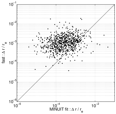
Figure 1: Accuracy of centroiding. This shows a comparison between our approach (fast) and the brute-force method, based the Sérsic profile.

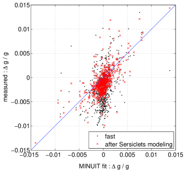
Figure 2: Accuracy of ellipticity measurements. This shows a comparison between our approach (fast) and the brute-force method, based the Sérsic profile. The dots are obtained using ellipticity algorithms decribed in Sec. 3, and crosses are results after using the nine lowest order sérsiclets basis functions constructed on a larger pixel grid. The side length of the larger pixel grid here is chosen to be ten times the half-light radius.

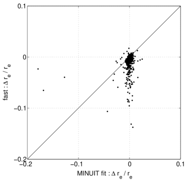
Figure 3: Accuracy of half-light radius determination. This shows a comparison between our approach (fast) and the brute-force method, based the Sérsic profile.

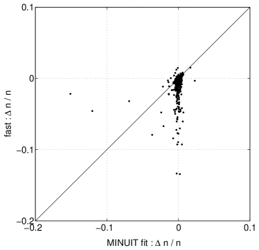
Figure 4: Accuracy of Sérsic index estimation. This shows a comparison between our approach (fast) and the brute-force method, based the Sérsic profile.

The accuracy of our methods is slightly worse than that of brute-force fitting. This can partially be attributed to the weight function used in our case (but not in brute-force fitting), as the outer region may play a non-negligible role. For more than 98% of the cases, $\Delta r/r_{e}$ from our method ranges between 0.01% and 1%.

Our estimation of the ellipticity deviates from the true ellipticity by less than 1% in most cases. Like any moments-based ellipticity estimation algorithms, our estimation of $g$ is biased when $g$ is large, due to the limited size of the image stamps used (side length 6$r_{50}$), resulting in moments calculations not converging completely. However, this bias is significantly reduced if we use our measured shape parameters to construct sérsiclets basis functions. The reproduced image is extroplated to a bigger size (side length 10$r_{50}$) so that subsequent moments calculations are not effected by the cut-off boundary. Then we run our algorithms again on the sérsiclets model. The crosses in Fig. 2 shows the $\Delta g/g$ estimated using the sérsiclets model with the nine lowest order basis functions build on a larger pixel grid. If we continue this process, each time we construct a new sérsiclets model, the data points in Fig. 2 continue to move toward the diagonal line until it reaches an unbiased state. Fig. 5 shows how $\Delta g/g$ varies with the true ellipticity for brute-force fitting, our algorithms, and our algorithms combined with sérsiclets modelling. The effectiveness of our approach in removing the bias at large ellipticity is clear. We also note that the wider spread of points in Fig. 5 (c) than in (a) is because that the model used in brute-force fitting is the same as what we used to simulate the images, in which case the brute-force fitting is superior over any other methods in terms of accuracy. But for real galaxies that are typically more complex than a simple Sérsic model (e.g., with bulge, bar, spiral arms, etc.), the basis functions will be more advantageous (e.g., Massey & Refregier, 2005; Andrae et al., 2011).

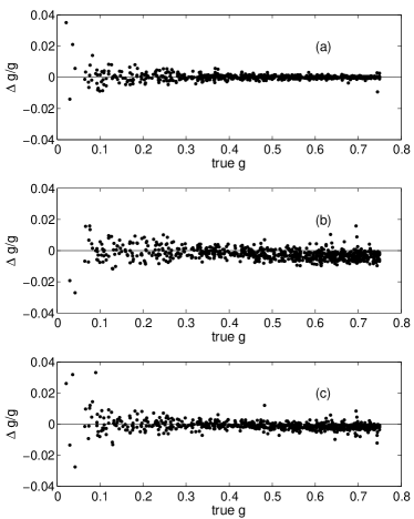
Figure 5: The dependence of ellipticity estimation accuracy on the size of ellipticity for (a) brute-force fitting, (b) our algorithms, and (c) our algorithms combined with sérsiclets modelling.

Because the centroid position and ellipticity are both fixed in the subsequent two-parameter fitting, the accuracy on $r_{e}$ and $n$ is worse than that of the brute-force approach, but is still well within 10% in most cases, as shown in Fig. 3 and Fig. 4. Most of the the outliers have small $r_{e}$ and big $n$. Their images are dominated just by several central pixels. This leads to relatively large uncertainty on the centrioding and then biases $r_{e}$ and $n$ bacause the strong degeneracy between these two parameters.

Going beyond individual parameters, we assess the quality of the fit to the overall light profile of a galaxy. Fig. 6 shows a comparison of the reduced $\chi^{2}$ values. When $N_{\rm pixel}$ is large, the ratio $\chi^{2}/N_{\rm pixel}$ is expected to be around unity if the estimation is unbiased. We found that the fit becomes progressively worse, as the Sérsic profile steepens (i.e., large $n$) and the size decreases. When the half-light radius approaches the size of a pixel, small error in centroiding may contribute significantly to the $\chi^{2}$ value. As one would have expected from the results in Fig. 2, constructing sérsiclets model using the estimated parameters reduces $\chi^{2}$, as shown by the crosses in Fig. 6.

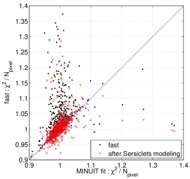
Figure 6: A comparison of the reduced $\chi^{2}$ values between our method (fast) and the brute-force method, based on the Sérsic profile. The dots are obtained using algorithms described in Secs. 2 and 3, and crosses are results after using the nine lowest order sérsiclets basis functions.

As for efficiency, on a single-core 2.2 GHz Intel CPU, it takes about 0.1 seconds to carry out centroiding and ellipticity measurement on one galaxy image and about 0.5 seconds to derive the remaining two parameters in the Sérsic model from profile fitting. In comparison, it takes about 6 seconds to process one galaxy image in the brute-force approach.

4.2 Star Images

We carried out similar tests with simulated star images, which are relevant to PSF modelling. Here, instead of using fitting programs like MINUIT, we developed faster numerical methods also to derive shape parameters from the moments of observed light profiles. Two kind of PSF profiles are considered here.

4.2.1 Gaussian profile

For the Gaussian profile,

$$I(r)=I_{0}e^{-\frac{r^{2}}{2\sigma^{2}}},$$ (14)

the zeroth and second order moments are

$$r_{0} =\int_{0}^{\infty}I(r)W(r)2\pi rdr,$$ (15)

$$r_{2} =\int_{0}^{\infty}I(r)W(r)2\pi r^{3}dr,$$ (16)

where the weight function is

$$W(r)=e^{-\frac{r^{2}}{2\sigma_{w}^{2}}}.$$ (17)

If we take $\sigma_{w}=\sigma$, we have

$$r_{0} =\pi\sigma^{2}I_{0},$$ (18)

$$r_{2} =\pi\sigma^{4}I_{0}.$$ (19)

Therefore,

$$\sigma =\sqrt{\frac{r_{2}}{r_{0}}},$$ (20)

$$I_{0} =\frac{r_{0}}{\pi\sigma^{2}}.$$ (21)

For the simulation, the half-light radius ($r_{50}$) is allowed to vary from 1.5 to 2.5 pixels. The ellipticity $g$ is limited to no greater than 0.25. We also let the centroid position vary, with respect to the origin, in the range of $\Delta x,\Delta y\in(-20,20)$. Gaussian noise is added to maintain a constant signal-to-noise ratio ($=300$) across an image. A total of 500 512 $\times$ 512 images are produced for the tests.

As for galaxies, we carry out centroiding and ellipticity determination with the methods described in Secs. 2 and 3. We then use Eqs. (20) and (21) to derive $\sigma$ and $I_{0}$ from the zeroth- and second-order moments. Setting $\sigma_{w}=\sigma$, we recalculate the moments. The iteration continues until the fractional change in $\sigma$ between two consecutive steps is less than $10^{-4}$ or the number of iterations reaches 20.

Fig. 7 shows a comparison between our approach and brute-force fitting in determining the half-light radius. In practice, the integrations of Eqs. (15) and (16) were done numerically. And this will bias the result because of pixelation, which has a prominent effect on small images. However, deviation is still within a few percent. The bias in the overall size can be roughly estimated as $\delta r_{50}^{2}/<r_{50}^{2}>\leavevmode\nobreak\ \lesssim 0.001$. This value is acceptable for weak lensing statistics (Paulin-Henriksson et al., 2009). The overall quality of the shape estimation is shown in Fig. 8.

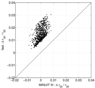
Figure 7: Half-light radius. This shows a comparison between our approach (fast) and the brute-force method, based the Gaussian profile.

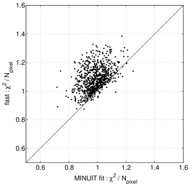
Figure 8: A comparison of the reduced $\chi^{2}$ values between our method (fast) and the brute-force method, based on the Gaussian profile.

4.2.2 Moffat profile

For the Moffat profile

$$I(r)=I_{0}\left(1+\left(\frac{r}{r_{d}}\right)^{2}\right)^{-\beta},$$ (22)

in addition to $r_{0}$ and $r_{2}$, we define

$$r_{4}=\int_{0}^{\infty}I(r)W(r)2\pi r^{5}dr,$$ (23)

where the weight function $W(r)$ is also of the Moffat shape,

$$W(r)=\left(1+\left(\frac{r}{r_{dw}}\right)^{2}\right)^{-3}.$$ (24)

If we take $r_{dw}=r_{d}$, we have

$$r_{0} =I_{0}\frac{\pi r_{d}^{2}}{\beta+2},$$ (25)

$$r_{2} =I_{0}\frac{\pi r_{d}^{4}}{(\beta+1)(\beta+2)},$$ (26)

$$r_{4} =I_{0}\frac{2\pi r_{d}^{6}}{\beta(\beta+1)(\beta+2)}.$$ (27)

Therefore,

$$\beta =\frac{1}{\frac{\displaystyle r_{4}r_{0}}{\displaystyle 2r_{2}^{2}}-1},$$ (28)

$$r_{d} =\sqrt{\frac{r_{2}}{r_{0}}(\beta+1)},$$ (29)

$$I_{0} =\frac{r_{0}(\beta+2)}{\pi r_{d}^{2}}.$$ (30)

As for the Gaussian profile, we have made 500 512 $\times$ 512 images. In the simulation, $\beta$ varies between 3 and 5. Similarly, we compute the centroid position, ellipticity, and $r_{d}$ from the moments by iterating on $r_{dw}$. The results are shown in Figs. (9) $-$ (11).

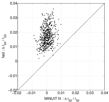
Figure 9: A comparison of the determination of half-light radius between our method (fast) and the brute-force method. This is based on the Moffat profile.

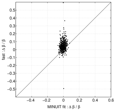
Figure 10: A comparison of the determination of Moffat power-law index between our method (fast) and the brute-force method.

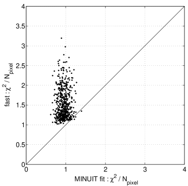
Figure 11: A comparison of the reduced $\chi^{2}$ values between our method (fast) and the brute-force method, based on the Moffat profile

Again, the biases in $r_{50}$ and $\beta$ are attributable to pixelation effects when we do the numerically integration of moments. The half-light radius $r_{50}$ is generally accurate to about 3-4% and the power-law index $\beta$ to less than 20%. As before, the bias in the overall size is roughly $\delta r_{50}^{2}/<r_{50}^{2}>\leavevmode\nobreak\ \lesssim 0.001$. Overall, the shape estimation is worse than in the case of Gaussian profiles (comparing Fig. 11 with Fig. 8). We found that the points with $\chi^{2}>1.5$ are dominated by realizations with $r_{d}<2$. This is because that the pixelation effect bias the moments two much. As same reason for Sérsic model, the Moffat profile also suffers from $r_{d}$-$\beta$ degeneracy. Therefore the problem here is more tough than that in Gaussian profile. In practice, for the data taken under similar weather conditions, we suggest to use several bright stars to derive $r_{d}$ and $\beta$ by using fitting process and then fix $\beta$ at the average value for other (fainter) stars. This could be a way out to break the degeneracy and to decrease the pixelation effect.

Based on the shape estimation algorithms described and tested above for the Gaussian and Moffat profiles, we have constructed two set of basis functions which are named gaussianlets and moffatlets, whose zeroth order profiles are Gaussian and Moffat, respectively (Li & Cui, 2012). The corresponding algorithms have been tested in the GRavitational lEnsing Accuracy Testing 2010 (GREAT10) Star Challenge (Kitching et al., 2010). Our gaussianlets worked very well with accuracy of $\sigma(e)\approx\sigma(R^{2})/R^{2}\approx 0.1\%$, where $e$ is the ellipticity and $R$ is the size (Kitching et al., 2012). But the moffatlets didn’t do very well especially when the PSF size is small.

5 Discussion

In this work, we have adapted the KSB algorithm for ellipticity determination. The new algorithm allows the use of elliptical weight functions and is applicable to highly elliptical shapes. This, combined with centroiding, makes it possible to eliminate four of the parameters from brute-force fitting. Consequently, less time is needed in searching for the remaining (shape) parameters. Overall, the efficiency is improved roughly by an order of magnitude.

We have tested our algorithms with simulated images that are representative of stars and galaxies. In general, our centroiding algorithm is accurate to well within 1%, although it is slightly worse than the brute-force fitting. For galaxy images, which are made with the Sérsic profile, our approach is relatively worse than brute-force fitting in determining the half-light radius and the Sérsic index. This is mainly due to the fact that the two parameters are tightly coupled, and then the fitting results will be biased by any small offset in centroiding. Overall, we can find very good fit to simulated galaxy profiles with our algorithms (as measured by the reduced $\chi^{2}$). The accuracy of parameter estimations is seen to be further improved when the algorithms are run on sérsiclets models with nine lowest order basis functions which are constructed with the estimated parameters as input. Given that galaxies are not perfectly Sérsic-like, our algorithms, combined with sérsiclets modelling, has unique advantages over other shape estimation techniques.

For star images, we have adopted profiles that are often used for PSF modelling, Gaussian and Moffat. In this case, we show that we can also derive the shape parameters directly from the moments of the light distribution, which improve the efficiency even further. However, for small images, pixelation leads to significant biases. Fortunately, the bias in the overall size is $\delta r_{50}^{2}/<r_{50}^{2}>\leavevmode\nobreak\ \lesssim 0.001$, which is still acceptable for weak lensing statistics. We participated in the GREAT10 star challenge. The results show that our methods performed quite well with Gaussian profiles but not as satisfactorily with Moffat profiles, particularly for data sets with stars of small radii. This tells us that the effects of pixelation and $r_{d}$-$\beta$ degeneracy must be taken into account for Moffat profile.

Like other algorithms, we also assume axisymmetric light distributions with constant ellipticity. In practice, this is known not to be the case for either galaxies or PSFs. In fact, the morphology of a galaxy or PSF can be quite complex.Therefore the use of simple spatial models leads to biases. The accuracy is expected to improve with more complicated spatial models. One possible option is to adopt appropriate basis functions, such as sérsiclets, moffatlets and gaussianlets, to reconstruct the light distribution. The approach described here shows its strong capability in providing input parameters for the basis functions. In spite of the deficiencies, our algorithms are very fast, which is important for future surveys, as the data volume is expected to increase drastically.

Appendix A The KSB algorithm with an elliptical weight function

Lets $W(R^{2})$ be an elliptical weight function, which is assumed to be converted by shear polarization $g_{w}$,

$$R^{2}=[(1-g_{w1})^{2}+g_{w2}^{2}]\theta^{2}_{1}+[(1+g_{w1})^{2}+g_{w2}^{2}]\theta^{2}_{2}-4g_{w2}\theta_{1}\theta_{2}.$$ (31)

Eq. (B5) in KSB95 now takes on the form

$$z_{lmij} =\frac{\partial[W({\mn@boldsymbol{\theta}})\theta_{i}\theta_{j}\theta_{m}]}{\partial\theta_{l}}$$

$$=W(\delta_{il}\theta_{j}\theta_{m}+\delta_{jl}\theta_{i}\theta_{m}+\delta_{ml}\theta_{i}\theta_{j})+W^{\prime}\theta_{i}\theta_{j}\theta_{m}\frac{\partial(R^{2})}{\partial\theta_{l}}.$$ (32)

Compared to the cases with circular weight function, the only change is that $2\theta_{l}$ is replaced with $\frac{\partial(R^{2})}{\partial\theta_{l}}$ in the terms that contain $W^{\prime}$, where the prime denotes differentiation with respect to $R^{2}$, i.e.,

$$\theta_{1} \longrightarrow\frac{1}{2}\frac{\partial(R^{2})}{\partial\theta_{1}}=A\theta_{1}-2g_{w2}\theta_{2},$$ (33)

$$\theta_{2} \longrightarrow\frac{1}{2}\frac{\partial(R^{2})}{\partial\theta_{2}}=B\theta_{2}-2g_{w2}\theta_{1},$$ (34)

where $A=1+g^{2}_{w}-2g_{w1}$ and $B=1+g^{2}_{w}+2g_{w1}$. $X^{SH}$ and $e^{SH}$ are now given by

$$X^{SH}=\frac{1}{T}\int d^{2}\theta f(\mn@boldsymbol{\theta})\left(\begin{array}[]{cc}2W\theta^{2}+2W^{\prime}(\theta_{1}^{2}-\theta_{2}^{2})(A\theta_{1}^{2}-B\theta_{2}^{2})&2W^{\prime}(\theta_{1}^{2}-\theta_{2}^{2})[(A+B)\theta_{1}\theta_{2}-2g_{w2}\theta^{2}]\\ 4W^{\prime}\theta_{1}\theta_{2}(A\theta_{1}^{2}-B\theta_{2}^{2})&2W\theta^{2}+4W^{\prime}\theta_{1}\theta_{2}[(A+B)\theta_{1}\theta_{2}-2g_{s2}\theta^{2}]\end{array}\right),$$ (35)

and

$$e^{SH}=2\left(\begin{array}[]{c}e_{1}\\ e_{2}\end{array}\right)+\frac{2}{T}\int d^{2}\theta f(\mn@boldsymbol{\theta})W^{\prime}\theta^{2}\left(\begin{array}[]{c}A\theta_{1}^{2}-B\theta_{2}^{2}\\ (A+B)\theta_{1}\theta_{2}-2g_{w2}\theta^{2}\end{array}\right).$$ (36)

Appendix B The iterative process for ellipticity determination

The KSB method is applicable only when the ellipticity of an object is small, i.e., $\phi_{,ij}$ in Eq. (B7) in KSB95 is small, so that the Taylor expansion is appropriate. However, galaxies are often highly elliptical. This appendix shows a derivation of $\Delta g=g-g_{w}$, where $g$ is the intrinsic ellipticity of an object and $g_{w}$ is the estimated ellipticity.

Let ${\mn@boldsymbol{\beta}}$ be the coordinates in the virtual plane with ellipticity $g_{w}$. ${\mn@boldsymbol{\beta}}$ and ${\mn@boldsymbol{\theta}}$ are related by

$${\mn@boldsymbol{\beta}}=C{\mn@boldsymbol{\theta}}.$$ (37)

where

$$C=\left(\begin{array}[]{cc}1-\gamma_{1}-(g_{w1}\gamma_{1}+g_{w2}\gamma_{2})&-\gamma_{2}+g_{w2}\gamma_{1}-g_{w1}\gamma_{2}\\ -\gamma_{2}-g_{w2}\gamma_{1}+g_{w1}\gamma_{2}&1+\gamma_{1}-(g_{w1}\gamma_{1}+g_{w2}\gamma_{2})\end{array}\right),$$ (38)

and

$$\gamma_{1}=\frac{\Delta g_{1}}{1-g^{2}_{w}},\quad\gamma_{2}=\frac{\Delta g_{2}}{1-g^{2}_{w}},$$ (39)

The surface brightness is conserved during the transformation defined in Eq. (38),

$$f_{w}({\mn@boldsymbol{\beta}})=f({\mn@boldsymbol{\theta}}).$$ (40)

Let $\psi=C^{-1}-1$, it follows that

$$f_{w}(\mn@boldsymbol{\beta})=f(C^{-1}\mn@boldsymbol{\beta})=f(\mn@boldsymbol{\beta}+\psi\mn@boldsymbol{\beta}).$$ (41)

Following the original KSB formalism,

$$Q^{w}_{ij}=Q_{ij}-\psi_{lm}Z_{lmij},$$ (42)

where $Z_{lmij}$ is defined in Eq. (B4) in KSB95. In their Eqs. (3.2) and (3.3), the difference in ellipticity $e$ between the real image with reduced shear $g$ and the virtual image with $g_{w}$ is easily related to $\delta Q_{ij}=Q_{ij}-Q^{w}_{ij}$. We then find that, in addition to the terms defined in Eqs. (35) and (36) in Appendix A, we now have the following extra terms on $X^{SH}$ and $e^{SH}$:

$$\Delta(X^{SH}) =\frac{1}{T}\int d^{2}\theta f(\mn@boldsymbol{\theta})\left(\begin{array}[]{cc}-g_{1}P_{1}-g_{2}P_{2}&g_{1}P_{2}-g_{2}P_{1}\\ -g_{1}P_{3}-g_{2}P_{4}&g_{1}P_{4}-g_{2}P_{3}\end{array}\right),$$ (45)

and

$$\Delta(e^{SH})=\frac{1}{T}\int d^{2}\theta f(\mn@boldsymbol{\theta})\left(\begin{array}[]{c}-g_{1}P_{5}-g_{2}P_{6}\\ g_{1}P_{6}-g_{2}P_{5}\end{array}\right),$$ (48)

where

$$P_{1} =4W(\theta_{1}^{2}-\theta_{2}^{2})+2W^{\prime}(\theta_{1}^{2}-\theta_{2}^{2})(A\theta_{1}^{2}+B\theta_{2}^{2}-4g_{2}\theta_{1}\theta_{2}),$$ (49)

$$P_{2} =4W\theta_{1}\theta_{2}+2W^{\prime}(\theta_{1}^{2}-\theta_{2}^{2})[(A-B)\theta_{1}\theta_{2}+2g_{2}(\theta_{1}^{2}-\theta_{2}^{2})],$$ (50)

$$P_{3} =8W\theta_{1}\theta_{2}+4W^{\prime}\theta_{1}\theta_{2}(A\theta_{1}^{2}+B\theta_{2}^{2}-4g_{2}\theta_{1}\theta_{2}),$$ (51)

$$P_{4} =-2W(\theta_{1}^{2}-\theta_{2}^{2})+4W^{\prime}\theta_{1}\theta_{2}[(A-B)\theta_{1}\theta_{2}+2g_{2}(\theta_{1}^{2}-\theta_{2}^{2})],$$ (52)

$$P_{5} =4W\theta^{2}+2W^{\prime}\theta^{2}(A\theta_{1}^{2}+B\theta_{2}^{2}-4g_{2}\theta_{1}\theta_{2}),$$ (53)

$$P_{6} =2W^{\prime}\theta^{2}[(A-B)\theta_{1}\theta_{2}+2g_{2}(\theta_{1}^{2}-\theta_{2}^{2})].$$ (54)

References

- Amara & Réfrégier (2008) Amara, A., & Réfrégier, A. 2008, MNRAS, 391, 228
- Andrae et al. (2011) Andrae, R., Melchior, P., & Jahnke, K. 2011, MNRAS, 417, 2465
- Bacon et al. (2000) Bacon, D. J., Refregier, A. R., & Ellis, R. S. 2000, MNRAS, 318, 625
- Bartelmann & Schneider (2001) Bartelmann, M., & Schneider, P. 2001, Phys. Rep., 340, 291
- Benjamin et al. (2007) Benjamin, J., Heymans, C., Semboloni, E., et al. 2007, MNRAS, 381, 702
- Bernstein & Jarvis (2002) Bernstein, G. M., & Jarvis, M. 2002, AJ, 123, 583
- Bosch (2010) Bosch, J. 2010, AJ, 140, 870
- Bridle et al. (2010) Bridle, S., Balan, S. T., Bethge, M., et al. 2010, MNRAS, 405, 2044
- Flusser & Suk (1998) Flusser, J., Suk, T., 1998, IEEE Trans. Pattern AnalysisMachine Intelligence, 20, 590
- Gadotti (2009) Gadotti, D. A. 2009, MNRAS, 393, 1531
- Heymans et al. (2006) Heymans, C., Van Waerbeke, L., Bacon, D., et al. 2006, MNRAS, 368, 1323
- Hirata & Seljak (2003) Hirata, C., & Seljak, U. 2003, MNRAS, 343, 459
- Hoekstra et al. (1998) Hoekstra, H., Franx, M., Kuijken, K., & Squires, G. 1998, ApJ, 504, 636
- James & Roos (1975) James, F., & Roos, M. 1975, Comput. Phys. Commun. 10, 343
- Kaiser et al. (1995) Kaiser, N., Squires, G., & Broadhurst, T. 1995, ApJ, 449, 460
- Kaiser (2000) Kaiser, N. 2000, ApJ, 537, 555
- Kennicutt (1998) Kennicutt, R. C., Jr 1998, ARA&A, 36, 189
- Kitching et al. (2008) Kitching, T. D., Miller, L., Heymans, C. E., van Waerbeke, L., & Heavens, A. F. 2008, MNRAS, 390, 149
- Kitching et al. (2012) Kitching, T. D., et al., 2012 in preparation
- Kitching et al. (2010) Kitching, T., Amara, A., Gill, M., et al. 2010, arXiv:1009.0779
- Li & Cui (2012) Li, G. L., & Cui, W. 2012 in preparation
- Luppino & Kaiser (1997) Luppino, G. A., & Kaiser, N. 1997, ApJ, 475, 20
- MacArthur et al. (2003) MacArthur, L. A., Courteau, S., & Holtzman, J. A. 2003, ApJ, 582, 689
- Massey & Refregier (2005) Massey, R. & Refregier, A. 2005, MNRAS, 359, 1277
- Massey et al. (2007) Massey, R., Heymans, C., Bergé, J., et al. 2007, MNRAS, 376, 13
- Melchior et al. (2009) Melchior, P., Andrae, R., Maturi, M., & Bartelmann, M. 2009, A&A, 493, 727
- Melchior et al. (2010) Melchior, P., Böhnert, A., Lombardi, M., & Bartelmann, M. 2010, A&A, 510, A75
- Melchior et al. (2011) Melchior, P., Viola, M., Schäfer, B. M., & Bartelmann, M. 2011, MNRAS, 412, 1552
- Miller et al. (2007) Miller, L., Kitching, T. D., Heymans, C., Heavens, A. F., & van Waerbeke, L. 2007, MNRAS, 382, 315
- Ngan et al. (2009) Ngan, W., van Waerbeke, L., Mahdavi, A., Heymans, C., & Hoekstra, H. 2009, MNRAS, 396, 1211
- Paulin-Henriksson et al. (2009) Paulin-Henriksson, S., Refregier, A., & Amara, A. 2009, A&A, 500, 647
- Refregier (2003) Refregier, A. 2003, MNRAS, 338, 35
- Refregier & Bacon (2003) Refregier, A. & Bacon, D. 2003, MNRAS, 338, 48
- Sérsic (1968) Sérsic, J.L. 1968, Atlas de galaxias australes. Obser. Astron., Córdoba, Argentina
- Van de Wel et al. (2010) Van der Wel, A., Bell, E. F., Holden, B. P., Skibba, & R. A., Rix, H. 2010, ApJ, 714, 1779
- Viola et al. (2011) Viola, M., Melchior, P., & Bartelmann, M. 2011, MNRAS, 410, 2156
- Voigt & Bridle (2010) Voigt, L. M., & Bridle, S. L. 2010, MNRAS, 404, 458
- Wang et al. (2012) Wang, J., Kauffmann, G., Overzier, R., et al. 2012, MNRAS, 423, 3486