Certified Approximation of Parametric Space Curves
with Cubic B-spline Curves

Abstract

Approximating complex curves with simple parametric curves is widely used in CAGD, CG, and CNC. This paper presents an algorithm to compute a certified approximation to a given parametric space curve with cubic B-spline curves. By certified, we mean that the approximation can approximate the given curve to any given precision and preserve the geometric features of the given curve such as the topology, singular points, etc. The approximated curve is divided into segments called quasi-cubic Bézier curve segments which have properties similar to a cubic rational Bézier curve. And the approximate curve is naturally constructed as the associated cubic rational Bézier curve of the control tetrahedron of a quasi-cubic curve. A novel optimization method is proposed to select proper weights in the cubic rational Bézier curve to approximate the given curve. The error of the approximation is controlled by the size of its tetrahedron, which converges to zero by subdividing the curve segments. As an application, approximate implicit equations of the approximated curves can be computed. Experiments show that the method can approximate space curves of high degrees with high precision and very few cubic Bézier curve segments.

1 Introduction

Parametric curves are widely used in different fields such as computer aided geometric design (CAGD), computer graphics (CG), computed numerical control (CNC) systems [1, 2]. One basic problem in the study of parametric curves is to approximate the curve with lower degree curve segments. For a given digital curve, there exist methods to find such approximate curves efficiently [3, 4, 5, 6]. If the curve is given by explicit expressions, either parametric or implicit, these methods are still usable. However, some important geometric features such as singular points cannot be preserved. In this paper, we will focus on computing approximate curves which can approximate the given curve to any precision and preserve the topology and certain geometric features of the given space curve. Such an approximate curve is called a certified approximation. Here, the geometric features include cusps, self-intersected points, inflection points, torsion vanishing points, as well as the segmenting points and the left(right) Frenet frames of these points.

There are lots of papers tried to approximate a smooth parametric curve segment [1, 7, 8, 9, 10, 11, 12, 13, 14]. Among them, Geometric Hermite Interpolation (GHI) is a typical method for the curve approximation. Degen [8] presented an overview over the developments of geometric Hermite approximation theory for planar curves. Several 2D interpolation schemes to produce curves close to circles were proposed in [9]. The certified approximation were considered by some authors and they focused on the case of planar curves [15, 16, 17, 18].

For space curves, Hijllig and Koch [10] improved the standard cubic Hermite interpolation with approximation order five by interpolating a third point. Xu and Shi [11] considered the GHI for space curves by parametric quartic Bézier curve. Pelosi et al. [12] discussed the problem of Hermite interpolation by using PH cubic segments. Chen et al. [14] enhanced the GHI by adding an inner tangent point and the approximation was then more accurate. These methods were mainly designed for the local approximation of a parametric curve segment. The approximate curves obtained generally cannot preserve geometric features and topologies for the global approximation. The algorithms had to be improved to meet certain special conditions. For instance, Wu et al [19] presented an algorithm to preserve the topology of voxelisation and Chen et al [20] gave the formula of the intersection curve of two ruled surfaces by the bracket method. As a further development for certified approximation, more properties such as the topology and singularities of the curve need to be discussed in the approximation process. We would like to give the local approximation with certain restrictions. And the local approximation methods can then be used in the global certified approximation naturally.

The certified approximation is also based on the topology determination. For implicit curves, the problem of topology determination was studied in some papers such as [21, 22, 23, 24]. Efficient algorithms were proposed in [25] and [26] to compute the real singular points of a rational parametric space curve by the $\mu$-basis method and the generalized $D$-resultant method respectively. An algorithm was proposed to compute the topology for a rational parametric space curve [27]. However, even we have the methods to determine the topology of space curves and the methods to approximate the space curves with free form curves, the combination of them is not straightforward. The topology may change while the line edges in topology graph are replaced by the approximate free form curve segments. For example, some knots may be brought in or lost such that the crossing number of the approximate curve is not equivalent to the approximated curve.

In this paper, we compute a certified approximation to a given parametric space curve with a rational cubic B-spline curve based on the topology. The cubic rational Bézier curve is taken as the approximate curve segment because it is the simplest non-planar curve and has nice properties [28, 29]. The presented method consists of two major steps.

In the first step, the given space curve segment is divided into sub-segments which have similar properties to a cubic rational Bézier curve. Such curve segments are called quasi-cubic Bézier curves. The preliminary work of our division procedure is to compute the singular points and the topology graph of the given curve, which have already been studied in [30, 25, 26, 27]. Inflection points and torsion vanishing points of the curve are also added as character points. We further divide the curve segments to ensure that the subdivided curve segments have similar properties to a cubic Bézier curve. For instance, each curve segment has an associated control tetrahedron whose four vertices consist of the two endpoints of the curve segment and the two intersection points of the tangent lines and the osculating planes at the different endpoints respectively. And the curve segment is inside its associated control tetrahedron. Furthermore, we need to ensure some monotone properties about the associated control tetrahedron, which are necessary for the convergence of the algorithm. The tetrahedrons are then just the control polytope of the approximate cubic Bézier curves. In other words, the approximate curve is controlled by the sequence of the tetrahedrons. And this property ensure the topological isotopy for the approximated and approximate curves. Some more careful discussions are proposed for both cubic Bézier and quasi-cubic curve segments.

In the second step of the algorithm, we use a cubic rational Bézier spline to approximate a quasi-cubic Bézier curve obtained in the first step. Some different approximation methods can be used here such as GHI with inner tangent points [14]. However, as we mentioned, a quasi-cubic Bézier curve has an associated control tetrahedron. The associated cubic rational Bézier curve of this tetrahedron is naturally used as the approximate curve. So, each curve segment and its approximated cubic curve segment share the same control tetrahedron. A novel method, called shoulder point approximation, is proposed to select parameters in the cubic Bézier curve so that it can optimally approximate the given curve segment. If the distance between the two curve segments is larger than the given precision, we further subdivide the given curve segment and approximate each sub-segment similarly. The error of the approximation is controlled by the size of the associated tetrahedrons, which are proved to converge to zero. In the subdivision process, there is one important difference between our algorithm with the others. We only need to check the collision of the sub-tetrahedrons subdivided from which are the intersected before the subdivision, since the sub-tetrahedrons are included in its father tetrahedrons. In general algorithms, one has to check the collision of all pair of the approximate curve segments or their control polytopes after a subdivision. Finally, the rational cubic Bézier curves are converted to a $C^{1}$ rational B-spline with a proper knot selection and used as the final approximate curve. After a cubic parametric approximate segment is computed, we can compute its algebraic variety using the $\mu$-basis method [31], which can be used as the approximate implicit equations for the given parametric curve.

The proposed method is implemented and experimental results show that the method can be used to compute certified approximate curves to high degree space curves efficiently. The computed rational B-spline has very few pieces and can approximate the given curves with high precision.

The rest of this paper is organized as follows. In Section 2, some notations and preliminary results are given. In Section 3, we give the algorithm to compute the dividing points such that each divided segment is a quasi-cubic curve. In Section 4, the method of parameter selection for the cubic rational Bézier segments is proposed and then an algorithm based on shoulder point approximation is given. We also prove that the termination of the algorithm. The final algorithm is given in Section 5, and some examples are used to illustrate the algorithm. In section 6, the paper is concluded.

2 Preliminaries

Basic notations and preliminary results about rational parametric curves and cubic Bézier curves are presented in this section.

2.1 Basic notations

A parametric space curve is defined as

$${\mathbf{r}}(t)=(x(t),y(t),z(t)),$$ (2.1)

where $x(t),y(t),z(t)\in\mathbb{Q}(t)$ and $\mathbb{Q}$ is the field of rational numbers. In the univariate case, Lüroth’s theorem provides a proper reparametrization algorithm and some improved algorithms which can also be found such as [30]. So we assume that (2.1) is a proper parametric curve in an interval $[0,1]$ since any interval $[a,b]$ can be transformed to $[0,1]$ by a parametric transformation $t\leftarrow\frac{t-a}{b-a}$. Further, the denominators of (2.1) are assumed to have no real roots in $[0,1]$.

The tangent vector of ${\mathbf{r}}(t)$ is ${\mathbf{r}}^{\prime}(t)=(x^{\prime}(t),y^{\prime}(t),z^{\prime}(t))$ and the tangent line of ${\mathbf{r}}(t)$ at a point ${\mathbf{r}}(t_{0})$ is ${\mathbf{T}}(t_{0})={\mathbf{r}}(t_{0})+\lambda{\mathbf{r}}^{\prime}(t_{0}),\lambda\in\mathbb{Q}$. A point ${\mathbf{r}}(t_{0})$ is called a singular point if it corresponds to more than one parameters with multiplicities counted. A singular point is called a cusp if ${\mathbf{r}}^{\prime}(t_{0})$ is the vector of zeros, which means that $t_{0}$ is a multiple parameter; otherwise, it is an ordinary singular point [26]. The curvature and torsion of the curve are

$$\kappa(t)=\frac{\|{\mathbf{r}}^{\prime}(t)\times{\mathbf{r}}^{\prime\prime}(t)\|}{\|{\mathbf{r}}^{\prime}(t)\|^{3}},\ \tau(t)=\frac{({\mathbf{r}}^{\prime},{\mathbf{r}}^{\prime\prime},{\mathbf{r}}^{\prime\prime\prime})}{\|{\mathbf{r}}^{\prime}\times{\mathbf{r}}^{\prime\prime}\|}.$$

A point is called an inflection if its curvature is zero and called torsion vanishing point if its torsion is zero. All these points are called character points of the curve, and ${\mathbf{r}}(t)$ is a normal curve if it has a finite number of character points. A rational space curve is always a normal curve. In this paper, we assume that $\kappa(t)\not\equiv 0$ and $\tau(t)\not\equiv 0$, which means that the curve is not a planar curve.

If ${\mathbf{r}}(t_{0})$ is not a character point, then the Frenet frame at ${\mathbf{r}}(t_{0})$ can be defined as ${\mathcal{F}}(t_{0}):=\{{\mathbf{r}}(t_{0});\boldsymbol{\alpha}(t_{0}),\boldsymbol{\beta}(t_{0}),\boldsymbol{\gamma}(t_{0})\}$ where $\boldsymbol{\alpha}(t_{0})=\frac{{\mathbf{r}}^{\prime}(t_{0})}{\|{\mathbf{r}}^{\prime}(t_{0})\|}$, $\boldsymbol{\beta}(t_{0})=\boldsymbol{\gamma}(t_{0})\times\boldsymbol{\alpha}(t_{0})$, $\boldsymbol{\gamma}(t_{0})=\frac{{\mathbf{r}}^{\prime}(t_{0})\times{\mathbf{r}}^{\prime\prime}(t_{0})}{\|{\mathbf{r}}^{\prime}(t_{0})\times{\mathbf{r}}^{\prime\prime}(t_{0})\|}$ are the unit tangent vector, unit principal normal vector, and unit bi-normal vector, respectively. And the osculating plane is $O(t_{0}):=((x,y,z)-{\mathbf{r}}(t_{0}))\cdot\boldsymbol{\gamma}(t_{0})=0$.

For a point with $\kappa(t_{0})=0$, the bi-normal vector is not defined, neither is the osculating plane. Here, we define them using limit. Consider the limit $\lim_{t\to t_{0}}\boldsymbol{\gamma}(t)$ of the bi-normal vector at $t_{0}$. Since the left limit and the right limit are generally different, we define the left bi-normal vector and the right bi-normal vector as $\boldsymbol{\gamma}^{-}(t_{0}):=\lim_{t\to t_{0}-0}\boldsymbol{\gamma}(t)$ and $\boldsymbol{\gamma}^{+}(t_{0}):=\lim_{t\to t_{0}+0}\boldsymbol{\gamma}(t)$ respectively. The limitations always exist if ${\mathbf{r}}(t)$ is a rational space curve of form (2.1). As a consequence, the left and right osculating planes at $t_{0}$ are $O^{-}(t_{0}):=((x,y,z)-{\mathbf{r}}(t_{0}))\cdot\boldsymbol{\gamma}^{-}=0$ and $O^{+}(t_{0}):=((x,y,z)-{\mathbf{r}}(t_{0}))\cdot\boldsymbol{\gamma}^{+}=0.$ If the $\kappa(t_{0})\neq 0$, one can find that $\boldsymbol{\gamma}^{+}(t_{0})=\boldsymbol{\gamma}^{-}(t_{0})$ and $O^{+}(t_{0})=O^{-}(t_{0})$.

Similarly, if $t_{0}$ is at a cusp, we define the left and right tangent vectors as $\boldsymbol{\alpha}^{-}(t_{0}):=\lim_{t\to t_{0}-0}\boldsymbol{\alpha}(t)$ and $\boldsymbol{\alpha}^{+}(t_{0}):=\lim_{t\to t_{0}+0}\boldsymbol{\alpha}(t)$, respectively. Hence, the corresponding left and right principal vectors are $\boldsymbol{\beta}^{-}(t_{0}):=\boldsymbol{\gamma}^{-}(t_{0})\times\boldsymbol{\alpha}^{-}(t_{0})$ and $\boldsymbol{\beta}^{+}(t_{0}):=\boldsymbol{\gamma}^{+}(t_{0})\times\boldsymbol{\alpha}^{+}(t_{0})$. We also denote the left and right tangent lines as ${\mathbf{T}}^{-}(t_{0})={\mathbf{r}}(t_{0})+\lambda\boldsymbol{\alpha}^{-}(t_{0})$ and ${\mathbf{T}}^{+}(t_{0})={\mathbf{r}}(t_{0})+\lambda\boldsymbol{\alpha}^{+}(t_{0})$ where $\lambda$ is the real number parameter. Then, a rational parametric curve ${\mathbf{r}}(t)$ always has left and right Frenet frames.

2.2 Rational cubic Bézier curve

A rational Bézier curve with degree $n$ has the following form

$${\mathbf{p}}(t)=\frac{\sum_{i=0}^{n}\omega_{i}{\mathbf{p}}_{i}B_{i}^{n}(t)}{\sum_{i=0}^{n}\omega_{i}B_{i}^{n}(t)},\ t\in[0,1],$$

where $\omega_{i}\geq 0$ are associated weights of the control points ${\mathbf{p}}_{i}\in\mathbb{R}^{3}$ and $B_{i}^{n}(t)=\binom{n}{i}(1-t)^{n-i}t^{i}$. When $n=3$, it defines a cubic rational Bézier curve where $\lozenge{\mathbf{p}}_{0}{\mathbf{p}}_{1}{\mathbf{p}}_{2}{\mathbf{p}}_{3}$ is called the control tetrahedron of ${\mathbf{p}}(t)$. One can set the weight $\omega_{0}=\omega_{3}=1$ up to a parametric transformation. We now consider the cubic curve and omit superscript $3$ from $B_{i}^{3}(t)$

$${\mathbf{p}}(t)=\frac{{\mathbf{p}}_{0}B_{0}(t)+\omega_{1}{\mathbf{p}}_{1}B_{1}(t)+\omega_{2}{\mathbf{p}}_{2}B_{2}(t)+{\mathbf{p}}_{3}B_{3}(t)}{B_{0}(t)+\omega_{1}B_{1}(t)+\omega_{2}B_{2}(t)+B_{3}(t)},\ t\in[0,1].$$ (2.2)

The rational cubic Bézier curve (2.2) has the following properties.

Lemma 2.1

Let ${\mathbf{p}}(t)$ be a non-planar cubic rational curve of the form (2.2). Then

1)

${\mathbf{p}}(t)$ passes through the endpoints ${\mathbf{p}}_{0},{\mathbf{p}}_{3}$ with the corresponding tangent directions ${\mathbf{p}}^{\prime}(0)$ and ${\mathbf{p}}^{\prime}(1)$ parallel to ${\mathbf{p}}_{0}{\mathbf{p}}_{1}$ and ${\mathbf{p}}_{2}{\mathbf{p}}_{3}$ respectively.

2)

${\mathbf{p}}_{0}{\mathbf{p}}_{1}{\mathbf{p}}_{2}$ and ${\mathbf{p}}_{1}{\mathbf{p}}_{2}{\mathbf{p}}_{3}$ are the osculating planes of ${\mathbf{p}}(t)$ at the endpoints ${\mathbf{p}}_{0}$ and ${\mathbf{p}}_{3}$, respectively.

3)

${\mathbf{p}}(t)$ lies inside its control tetrahedron $\lozenge{\mathbf{p}}_{0}{\mathbf{p}}_{1}{\mathbf{p}}_{2}{\mathbf{p}}_{3}$.

4)

${\mathbf{p}}(t)$ has no singular points and $\kappa(t)\neq 0,\tau(t)\neq 0$ in $[0,1]$.

5)

For any $t^{\star}_{1}<t^{\star}_{2}\in[0,1]$, the control tetrahedron of ${\mathbf{p}}^{\star}(t)={\mathbf{p}}(t),t\in[t^{\star}_{1},t^{\star}_{2}]$ is inside the control tetrahedron of ${\mathbf{p}}(t)$ .

6)

$\|{\mathbf{p}}_{0}{\mathbf{p}}_{01}\|,\|{\mathbf{p}}_{1}{\mathbf{p}}_{12}\|$, and $\|{\mathbf{p}}_{2}{\mathbf{p}}_{23}\|$ are strictly monotone for $t^{\star}\in(0,1)$ where ${\mathbf{p}}_{01},{\mathbf{p}}_{12}$, and ${\mathbf{p}}_{23}$ are the intersection points of the osculating plane $O(t^{\star})$ with ${\mathbf{p}}_{0}{\mathbf{p}}_{1},{\mathbf{p}}_{1}{\mathbf{p}}_{2},$ and ${\mathbf{p}}_{2}{\mathbf{p}}_{3}$ respectively.

7)

$\|{\mathbf{p}}_{0}{\mathbf{p}}_{03}\|$ and $\|{\mathbf{p}}_{1}{\mathbf{p}}_{12}\|$ are strictly monotone for $t^{\star}\in(0,1)$ where ${\mathbf{p}}_{03}={\mathbf{p}}_{1}{\mathbf{p}}_{2}{\mathbf{p}}(t^{\star})\bigcap{\mathbf{p}}_{0}{\mathbf{p}}_{3}$ and ${\mathbf{p}}_{12}={\mathbf{p}}_{0}{\mathbf{p}}_{3}{\mathbf{p}}(t^{\star})\bigcap{\mathbf{p}}_{1}{\mathbf{p}}_{2}$.

Proof 1

Properties 1), 2) and 3) are basic properties of Bézier curves and the proof can be founded in [1]. They also can be checked directly.

For 4), Li and Cripps shown that there is no cusps and inflection points for a non-degenerate rational cubic space curves in [32], and the torsion can be checked directly. Wang et al. also proved that a cubic space curve has no singular points by moving planes method in [25].

5) can be proved by a successive Decasteljau subdivision [1]. The control tetrahedron of ${\mathbf{p}}^{\star}_{1}(t),t\in[t_{1}^{\star},1]$ is inside the control tetrahedron of ${\mathbf{p}}(t)$. Successively, the control tetrahedron of ${\mathbf{p}}^{\star}(t),t\in[t_{1}^{\star},t_{2}^{\star}]$ lies in the control tetrahedron of ${\mathbf{p}}^{\star}_{1}(t)$.

Property 6) can be derived from the above five properties. Also this property is a special case of the following Theorem 3.10 in this paper.

For 7), it is sufficient to prove that the planes ${\mathbf{p}}_{1}{\mathbf{p}}_{2}{\mathbf{p}}(t^{\star})$ and ${\mathbf{p}}_{0}{\mathbf{p}}_{3}{\mathbf{p}}(t^{\star})$ do not touch ${\mathbf{p}}(t^{\star})$ with $t^{\star}\in(0,1)$, respectively. Since ${\mathbf{p}}_{0}{\mathbf{p}}_{3}{\mathbf{p}}(t^{\star})$ passes through ${\mathbf{p}}_{0},{\mathbf{p}}_{3}$ and ${\mathbf{p}}(t)$ is cubic, ${\mathbf{p}}_{0}{\mathbf{p}}_{3}{\mathbf{p}}(t^{\star})$ cannot have any tangent point different from ${\mathbf{p}}_{0},{\mathbf{p}}_{3}$. Supposing the plane ${\mathbf{p}}_{1}{\mathbf{p}}_{2}{\mathbf{p}}(t^{\star})$ touches ${\mathbf{p}}(t^{\star})$ at $t^{\star}\in(0,1)$, the osculating plane $O(t^{\star})$ must intersects ${\mathbf{p}}_{1}{\mathbf{p}}_{2}{\mathbf{p}}(t^{\star})$ with the tangent line ${\mathbf{T}}(t^{\star})$. By 6), ${\mathbf{T}}(t^{\star})$ must intersect ${\mathbf{p}}_{1}{\mathbf{p}}_{2}$ which is the intersection line of $O(0),O(1)$. However, according to Decasteljau subdivision, the intersection point of ${\mathbf{T}}(t^{\star})$ and $O(0)$ is always different from that of ${\mathbf{T}}(t^{\star})$ and $O(1)$. Then there is a contradiction.

The shoulder point of a cubic Bézier curve will play an important role [28]. The definition is given below.

Definition 2.2

Let ${\mathbf{p}}(t)$ be a curve of the form (2.2). Its shoulder point ${\mathbf{s}}$ is defined as intersection point of ${\mathbf{p}}(t)$ and the plane ${\mathbf{p}}_{1}{\mathbf{p}}_{2}{\mathbf{p}}_{M}$ where ${\mathbf{p}}_{M}=({\mathbf{p}}_{0}+{\mathbf{p}}_{3})/2$ (Figure 1).

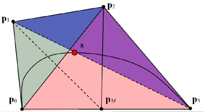
Figure 1: Shoulder point of a Bézier cubic curve

Proposition 2.3

Let ${\mathbf{s}}$ be the shoulder point of ${\mathbf{p}}(t)$. Then ${\mathbf{s}}={\mathbf{p}}(1/2)=\lambda_{1}{\mathbf{p}}_{1}+\lambda_{2}{\mathbf{p}}_{2}+(1-\lambda_{1}-\lambda_{2}){\mathbf{p}}_{M}$ where $\lambda_{1}={\frac{3\omega_{1}}{2+3\,\omega_{1}+3\,\omega_{2}}}$, $\lambda_{2}={\frac{3\omega_{2}}{2+3\,\omega_{1}+3\,\omega_{2}}}$.

Proof 2

By 7) of Lemma 2.1, there exists a unique intersection point of ${\mathbf{p}}(t)$ and the plane ${\mathbf{p}}_{1}{\mathbf{p}}_{2}{\mathbf{p}}_{M}$. And $\lambda_{1},\lambda_{2}$ and $1-\lambda_{1}-\lambda_{2}$ are just the area coordinates of ${\mathbf{s}}$ in the triangle ${\mathbf{p}}_{1}{\mathbf{p}}_{2}{\mathbf{p}}_{M}$. More details can be found in [28].

It is known that the curve is closer to the control point when its associated weight is greater. We now consider the point which has the maximum distance to the planes $P_{1}={\mathbf{p}}_{0}{\mathbf{p}}_{2}{\mathbf{p}}_{3}$ and $P_{2}={\mathbf{p}}_{0}{\mathbf{p}}_{1}{\mathbf{p}}_{3}$ respectively.

Definition 2.4

Let ${\mathbf{r}}(t),t\in[0,1]$ be a curve segment on the same side of a plane $Q$ with the two endpoints on $Q$. For another plane $R$ parallel to $Q$, a tangent point of ${\mathbf{r}}(t)$ with the plane $R$ is called a parallel point of ${\mathbf{r}}(t)$ associated to the plane $Q$.

According to the definition, a parallel point should satisfy

$$|{\mathbf{r}}^{\prime}(t),{\mathbf{q}}_{1}-{\mathbf{q}}_{0},{\mathbf{q}}_{2}-{\mathbf{q}}_{0}|=0,$$ (2.3)

where ${\mathbf{q}}_{0},{\mathbf{q}}_{1}$ and ${\mathbf{q}}_{2}$ are three non co-linear points on $Q$. In general, there may be several parallel points for a curve segment and a fixed plane. However, for the rational cubic curve segment (2.2), there is a unique parallel point associated to $P_{1}={\mathbf{p}}_{0}{\mathbf{p}}_{2}{\mathbf{p}}_{3}$, and similarly, there is a unique parallel point associated to $P_{2}={\mathbf{p}}_{0}{\mathbf{p}}_{1}{\mathbf{p}}_{3}$.

Proposition 2.5

Let ${\mathbf{p}}(t)$ be a non-planar cubic rational curve of the form (2.2). Then there are unique parallel points associated to the planes $P_{1}$ and $P_{2}$ respectively, and they are points of ${\mathbf{p}}(t)$ having the maximal distance to $P_{1}$ and $P_{2}$ respectively.

Proof 3

By equation (2.3), we can find that $\frac{3t^{3}-6t^{2}+6t-2}{3t(t-1)^{2}}=\omega_{1}$ and $\frac{3t^{3}-3t^{2}+3t-1}{3t^{2}(t-1)}=\omega_{2}$ are the constraint equations for the parallel points associated to $P_{1}$ and $P_{2}$ respectively. They are two monotone functions for $t\in(0,1)$ with two asymptotes $t=0,1$. It means that for any weights there is only one parallel point associated to $P_{i}$. Furthermore, the parallel point has the maximal distance since the endpoints of the curve are on $P_{i}$.

3 Quasi-cubic segments on space parametric curves

In this section, we propose a method to divide a given curve ${\mathbf{r}}(t)$ into segments which have similar properties to cubic Bézier curves, which are called quasi-cubic Bézier segments and can be approximated by cubic rational Bézier curves nicely.

3.1 Conditions for subdivision

Let $t_{0},t_{1}$ be the endpoints of a curve segment ${\mathbf{r}}(t)$. We will define an associated tetrahedron for it. Let $O^{+}(t_{0})$ and $O^{-}(t_{1})$ be the right and left osculating planes at the endpoints respectively. We denote their intersection line as $L$, if they are not parallel. Since $L$ and the right tangent line ${\mathbf{T}}^{+}(t_{0})$ are coplanar, they intersect at a point ${\mathbf{r}}_{1}$ if they are not parallel. Similarly, $L$ and the right tangent line ${\mathbf{T}}^{-}(t_{1})$ intersect at a point ${\mathbf{r}}_{2}$ if they are not parallel. So we obtain an associated tetrahedron $\lozenge(t_{0},t_{1})=\lozenge{\mathbf{r}}_{0}{\mathbf{r}}_{1}{\mathbf{r}}_{2}{\mathbf{r}}_{3}$ where ${\mathbf{r}}_{0}={\mathbf{r}}(t_{0})$ and ${\mathbf{r}}_{3}={\mathbf{r}}(t_{1})$ if ${\mathbf{r}}_{1}\neq{\mathbf{r}}_{2}$.

We have shown that a cubic Bézier curve segment has eight properties in Lemma 2.1 and Proposition 2.5. In the following, we will show how to divide any given rational curve segment into sub-segments having similar properties.

Definition 3.1

A curve segment is called a quasi-cubic Bézier curve segment, or simply a quasi-cubic segment, if it has the eight properties in Lemma 2.1 and Proposition 2.5.

Theorem 3.2

Given ${\mathbf{r}}(t)$ and $t_{0}$, there always exists $t_{1}>t_{0}$ such that ${\mathbf{r}}(t),t\in[t_{0},t_{1}]$ is a quasi-cubic Bézier curve segment.

We leave the proof of this theorem at the end of the subsection 3.2.

Definition 3.3

Let ${\mathbf{r}}(t),t\in[t_{0},t_{1}]$ be a quasi-cubic segment. Then its associated cubic Bézier curve segment is defined by the associated tetrahedron of ${\mathbf{r}}(t)$, i.e., the control points are ${\mathbf{r}}_{0},{\mathbf{r}}_{1},{\mathbf{r}}_{2}$ and ${\mathbf{r}}_{3}$.

In order to divide the curve segment into quasi-cubic segments, we first add the inflection points and torsion vanishing points as the dividing points, denoted by ${\mathbb{P}}$. The parameters of these points can be computed by solving the real roots of $\kappa(t)\tau(t)=0$. The left and right Frenet frames are also needed. There are several efficient methods to find the real roots of a univariate polynomial [33, 34] and one can use the procedures realroot and isolate in Maple.

We need to find more dividing points. Fix a start point $t=t_{0}$, we now try to determine $t_{1}$ such that $t_{1}-t_{0}$ is as big as possible and the segment is included in its associated tetrahedron designed above. Several boundary parametric values to exclude some special points with respect to $t_{0}$ are computed in the following cases:

Condition I). Let $t^{\star}_{1}>t_{0}$ be its nearest parametric value from ${\mathbb{P}}$. Find $t_{1}\in(t_{0},t_{1}^{\star})$ such that $F_{1}(s_{1},s_{2}):=\boldsymbol{\alpha}^{+}(s_{1})\cdot\boldsymbol{\gamma}^{-}(s_{2})\neq 0$ and $F_{2}(s_{1},s_{2}):=\boldsymbol{\alpha}^{-}(s_{2})\cdot\boldsymbol{\gamma}^{+}(s_{1})\neq 0$ for any $t_{0}\leq s_{1}<s_{2}\leq t_{1}$, meaning that the right tangent vector $\boldsymbol{\alpha}^{+}(s_{1})$ is not parallel to the left osculating plane $O^{-}(s_{2})$ and the left tangent vector $\boldsymbol{\alpha}^{-}(s_{2})$ is not parallel to the left osculating plane $O^{+}(s_{1})$.

Since the curve is non-planar, $F_{i}(s_{1},s_{2}),i=1,2$ cannot be identically zero. We take a further look at the inequalities $F_{1}\neq 0,F_{2}\neq 0$. Since the derivative can be computed using limits, ${\mathbf{r}}(t)$ is differentiable to any order although the left and right derivative may be different. For conveniences, we omit the $+,-$ marks to distinguish between left and right derivatives. In what below, we give detailed analysis for $F_{1}$ and the analysis of $F_{2}$ is similar.

$$F_{1}(s_{1},s_{2})=\boldsymbol{\alpha}(s_{1})\cdot\boldsymbol{\gamma}(s_{2})=\frac{|{\mathbf{r}}^{\prime}(s_{1}),{\mathbf{r}}^{\prime}(s_{2}),{\mathbf{r}}^{\prime\prime}(s_{2})|}{\|{\mathbf{r}}^{\prime}(s_{1})\|\|{\mathbf{r}}^{\prime}(s_{2})\times{\mathbf{r}}^{\prime\prime}(s_{2})\|}.$$

Assuming $s_{1}=t_{0}+{\delta}_{1},s_{2}=s_{1}+{\delta}_{2},{\delta}_{1}\geq 0,{\delta}_{2}>0$, $F_{1}(s_{1},s_{2})$ is re-parameterized as

$$F_{1}({\delta}_{1},{\delta}_{2})=\frac{|{\mathbf{r}}^{\prime}(t_{0}+{\delta}_{1}),{\mathbf{r}}^{\prime}(t_{0}+{\delta}_{1}+{\delta}_{2}),{\mathbf{r}}^{\prime\prime}(t_{0}+{\delta}_{1}+{\delta}_{2})|}{\|{\mathbf{r}}^{\prime}(t_{0}+{\delta}_{1})\|\|{\mathbf{r}}^{\prime}(t_{0}+{\delta}_{1}+{\delta}_{2})\times{\mathbf{r}}^{\prime\prime}(t_{0}+{\delta}_{1}+{\delta}_{2})\|}.$$

Expanding the vectors of the numerator at $t=t_{0}+{\delta}_{1}$ as Taylor series ${\mathbf{r}}^{\prime}_{S}(t_{0}+{\delta}_{1}),{\mathbf{r}}^{\prime}_{S}(t_{0}+{\delta}_{1}+{\delta}_{2})$ and ${\mathbf{r}}^{\prime\prime}_{S}(t_{0}+{\delta}_{1}+{\delta}_{2})$ respectively, and combining them, we have

$$F_{1}({\delta}_{1},{\delta}_{2})=\frac{{\delta}_{2}^{2}|{\mathbf{r}}^{\prime}_{S}(t_{0}+{\delta}_{1}),\tilde{\mathbf{r}}^{\prime\prime}_{S}(t_{0}+{\delta}_{1}+{\delta}_{2}),\tilde{\mathbf{r}}^{\prime\prime\prime}_{S}(t_{0}+{\delta}_{1}+{\delta}_{2})|}{\|{\mathbf{r}}^{\prime}(t_{0}+{\delta}_{1})\|\|{\mathbf{r}}^{\prime}(t_{0}+{\delta}_{1}+{\delta}_{2})\times{\mathbf{r}}^{\prime\prime}(t_{0}+{\delta}_{1}+{\delta}_{2})\|},$$ (3.1)

where $\tilde{\mathbf{r}}^{\prime\prime}_{S}(t_{0}+{\delta}_{1}+{\delta}_{2})=({\mathbf{r}}^{\prime}_{S}(t_{0}+{\delta}_{1}+{\delta}_{2})-{\mathbf{r}}^{\prime}_{S}(t_{0}+{\delta}_{1}))/{\delta}_{2}$ and $\tilde{\mathbf{r}}^{\prime\prime\prime}_{S}(t_{0}+{\delta}_{1}+{\delta}_{2})=({\mathbf{r}}^{\prime\prime}(t_{0}+{\delta}_{1}+{\delta}_{2})-\tilde{\mathbf{r}}^{\prime\prime}_{S}(t_{0}+{\delta}_{1}+{\delta}_{2}))/{\delta}_{2}$. Furthermore, when ${\delta}_{2}=0$, $\tilde{\mathbf{r}}^{\prime\prime}_{S}(t_{0}+{\delta}_{1})={\mathbf{r}}^{\prime\prime}_{S}(t_{0}+{\delta}_{1})$ and $\tilde{\mathbf{r}}^{\prime\prime\prime}_{S}(t_{0}+{\delta}_{1})={\mathbf{r}}^{\prime\prime\prime}_{S}(t_{0}+{\delta}_{1})$.

Let $f_{1}({\delta}_{1},{\delta}_{2})=F_{1}({\delta}_{1},{\delta}_{2})/{\delta}_{2}^{2}$. Then $f_{1}({\delta}_{1},0)=\tau(t_{0}+{\delta}_{1})/\|{\mathbf{r}}^{\prime}(t_{0}+{\delta}_{1})\|$. $F_{1}({\delta}_{1},{\delta}_{2})=0$ is a planar curve in the plane of $({\delta}_{1},{\delta}_{2})$ which has two components: a double line ${\delta}_{2}^{2}=0$ and another planar curve $f_{1}({\delta}_{1},{\delta}_{2})=0$. That means $f_{1}=0$ intersects ${\delta}_{2}=0$ with the points which are exactly the torsion vanishing points $\tau(t_{0}+{\delta}_{1})=0$ of ${\mathbf{r}}(t)$. And we need not compute these points since they are already included in the separating points needed in the topology computation which is discussed in Section 3.3. Consider the intersection points of $f_{1}({\delta}_{1},{\delta}_{2})$ and ${\delta}_{1}=0$. We can find that the real roots of $f_{1}(0,{\delta}_{2})=0$ are associated to the vector $\boldsymbol{\alpha}(s_{1})={\mathbf{r}}^{\prime}(t_{0})$ just parallelling to the osculating plane $O(s_{2})=O(t_{0}+{\delta}_{2})$.

Thus, condition I) can be reduced to solve the following optimization problem

$$\begin{array}[]{cl}\min&{\delta}_{1}+{\delta}_{2}\\ \mbox{s.t.}&F_{1}({\delta}_{1},{\delta}_{2})=0,{\delta}_{1}\geq 0,{\delta}_{2}>0\end{array}$$ (3.2)

and then $t_{1}$ can be selected from $(t_{0},t_{0}+{\delta}_{1}+{\delta}_{2})$. There are numerical methods to solve the optimization problem. However, we prefer to solve it based on the above discussion since it is enough to get a boundary parametric value less than the exact solution of (3.2). We can find the positive real roots of $f_{1}({\delta}_{1},0)$ and $f_{1}(0,{\delta}_{2})$ for ${\delta}_{1}$ and ${\delta}_{2}$ respectively. Let ${\delta}_{1}^{\star}$ be the minimal one among all the real roots. Then ${\delta}_{1}+{\delta}_{2}={\delta}_{1}^{\star}$ defines a line. If the line does not intersect $f_{1}$ in the first quadrant, then $t_{1}$ can be in $(t_{0},t_{0}+{\delta}_{1}^{\star})$. This can be checked by finding the real roots of $f_{1}({\delta}_{1}^{\star}-{\delta}_{2},{\delta}_{2})=0$. Otherwise, set ${\delta}_{1}^{\star}\leftarrow{\delta}_{1}^{\star}/2$ and check the process repeatedly until the proper ${\delta}_{1}^{\star}$ is found. If $f_{1}({\delta}_{1},0)$ and $f_{1}(0,{\delta}_{2})$ have no positive real roots, ${\delta}_{1}^{\star}$ can be initialed as ${\delta}_{1}^{\star}=t_{1}^{\star}-t_{0}$.

Similarly, we can find such a ${\delta}_{2}^{\star}$ for $F_{2}$. Finally, let $t_{2}^{\star}=\min(t_{0}+{\delta}_{1}^{\star},t_{0}+{\delta}_{2}^{\star})$ be the boundary parametric value of $t_{1}$.

Remark 3.4

The function $F_{1}({\delta}_{1},{\delta}_{2})$ in (3.1) actually has a finite number of terms if the approximated curve ${\mathbf{r}}$ is a rational curve. If ${\mathbf{r}}$ is a parametric curve in elementary functions, $F_{1}({\delta}_{1},{\delta}_{2})$ will be in the series form. However, the problem (3.2) can still be solved using a numerical method. Starting with an initial value ${\delta}_{1}^{\star}$, we can find a boundary number by checking whether ${\delta}_{1}+{\delta}_{2}={\delta}_{1}^{\star}$ and $F_{1}({\delta}_{1},{\delta}_{2})$ have common points in the first quadrant with one of the directions $\{{\delta}^{0}\leftarrow{\delta}_{1}^{\star}/2,{\delta}^{0}\leftarrow 2{\delta}_{1}^{\star}\}$.

Further restrictions will be proposed afterward. We will omit the similar discussions and solving processes and give the conditions directly.

Condition II). Let $t_{2}^{*}$ be the parametric value $t_{1}$ computed in the above procedure. Find $t_{1}\in(t_{0},t_{2}^{\star})$ such that

$$F(s_{1},s_{2}):=\boldsymbol{\alpha}^{+}(s_{1})\times({\mathbf{r}}(s_{2})-{\mathbf{r}}(s_{1}))\cdot\boldsymbol{\alpha}^{-}(s_{2})\neq 0$$

for any $t_{0}\leq s_{1}<s_{2}\leq t_{1}$, which means that the right tangent line ${\mathbf{T}}^{+}(s_{1})$ and the left tangent line ${\mathbf{T}}^{-}(s_{2})$ are not coplanar.

Condition III). Let $t_{3}^{*}$ be the parametric value $t_{1}$ computed in the above procedure. We should find $t_{1}\in(t_{0},t_{3}^{\star})$ such that $F_{1}(s_{1},s_{2}):=O^{-}(s_{2})({\mathbf{r}}(s_{1}))\neq 0$ and $F_{2}(s_{1},s_{2}):=O^{+}(s_{1})({\mathbf{r}}(s_{2}))\neq 0$, which imply that ${\mathbf{r}}(s_{1})$ is not on the left osculating plane $O^{-}(s_{2})$ and ${\mathbf{r}}(s_{2})$ is not on the right osculating plane $O^{+}(s_{1})$.

Conditions I), II), and III) are used to guarantee that the tetrahedron $\lozenge{\mathbf{r}}_{0}{\mathbf{r}}_{1}{\mathbf{r}}_{2}{\mathbf{r}}_{3}$ is not degenerated to a plane polygon. However, these conditions are still not sufficient for the curve segment lying inside $\lozenge{\mathbf{r}}_{0}{\mathbf{r}}_{1}{\mathbf{r}}_{2}{\mathbf{r}}_{3}$. We will give one more condition such that the curve segment lies inside the tetrahedron and has only one parallel points associated to planes $P_{1}$ and $P_{2}$ respectively.

Let $\tilde{t}_{1}<t^{\star}_{4}$ where $t^{\star}_{4}$ is the parameter value obtained from III). Then the curve segment ${\mathbf{r}}(t),t\in[t_{0},\tilde{t}_{1}]$ satisfies the conditions of I) to III) and ${\mathbf{r}}(t)$ has no character points. We will try to find $t^{\star}\in(t_{0},\tilde{t}_{1}]$ such that for any $s_{1}<s_{2}<s_{3}\in[t_{0},t^{\star}]$, the tangent vectors $\boldsymbol{\alpha}(s_{1})$, $\boldsymbol{\alpha}(s_{2})$, and $\boldsymbol{\alpha}(s_{3})$ are not coplanar, i.e.,

$$|\boldsymbol{\alpha}(s_{1}),\boldsymbol{\alpha}(s_{2}),\boldsymbol{\alpha}(s_{3})|\neq 0.$$ (3.3)

The following lemma is needed for further discussion.

Lemma 3.5

For a fixed $t_{0}$ and $\forall\epsilon>0$, $F(s_{1},s_{2}):=|\boldsymbol{\alpha}(t_{0}),\boldsymbol{\alpha}(s_{1}),\boldsymbol{\alpha}(s_{2})|=0$ has solutions $(s_{1},s_{2})$ in $(0,\epsilon)^{2}$ if and only if ${\mathbf{r}}(t)$ is a planar curve.

Proof 4

It can be checked by expanding vectors to Taylor series which are partly illustrated above.

And the lemma also holds for $F$ mentioned in I) to III). It means that $F(s_{1},s_{2})$ has no branch segment on the first quadrant of the $(s_{1},s_{2})$ plane connecting the origin point.

Condition IV). Find $t^{\star}\in(t_{0},\tilde{t}_{1})$ such that $F:=|\boldsymbol{\alpha}(s_{1}),\boldsymbol{\alpha}(s_{2}),\boldsymbol{\alpha}(s_{3})|\neq 0$ for any $s_{1}<s_{2}<s_{3}\in[t_{0},t^{\star}]\subset[t_{0},\tilde{t}_{1}]$. That means ${\mathbf{r}}(t)$ does not have a triple of linear dependent tangents in $[t_{0},t^{\star}]$. Suppose $s_{1}=t_{0}+{\delta}_{1}$, $s_{2}=s_{1}+{\delta}_{2}$ and $s_{3}=s_{2}+{\delta}_{3}$ where ${\delta}_{1}\geq 0,{\delta}_{2}>0$ and ${\delta}_{3}>0$.

If ${\delta}_{1}>0$, then we need to find the least $t_{0}+{\delta}_{1}+{\delta}_{2}+{\delta}_{3}$ with $F({\delta}_{1},{\delta}_{2},{\delta}_{3})=0$, that is,

$$\begin{array}[]{rl}\min&{\delta}_{1}+{\delta}_{2}+{\delta}_{3}\\ \mbox{ s.t.}&F({\delta}_{1},{\delta}_{2},{\delta}_{3})=0,{\delta}_{1},{\delta}_{2},{\delta}_{3}>0.\end{array}$$

By Taylor expansion, we find that $F({\delta}_{1},{\delta}_{2},{\delta}_{3})$ has no branch passing through the $({\delta}_{i},{\delta}_{j})$ plane from the first octant in the space of $({\delta}_{1},{\delta}_{2},{\delta}_{3})$. Then we initialize ${\delta}_{i},i=1,2,3$ in the plane ${\delta}_{1}+{\delta}_{2}+{\delta}_{3}={\delta}_{1}^{\star}=\tilde{t}_{1}$ and check the intersection of the plane with $F$. Set the boundary parametric value $t_{51}^{\star}={\delta}_{1}^{\star}$ if there is no intersection; otherwise set ${\delta}_{1}^{\star}\leftarrow{\delta}_{1}^{\star}/2$ and repeat the checking process.

If ${\delta}_{1}=0$, then $F({\delta}_{2},{\delta}_{3})$ degenerates to the special case mentioned in Lemma 3.5 and we can find a boundary parametric value as $t_{52}^{\star}$. Finally, let $t^{\star}=\min(t_{51}^{\star},t_{52}^{\star})$.

We have the following key theorem.

Theorem 3.6

Let $t^{\star}$ be found by the above process. For any $\epsilon>0$, $t_{1}=t^{\star}-\epsilon>t_{0}$, the associated tetrahedron $\lozenge{\mathbf{r}}_{0}{\mathbf{r}}_{1}{\mathbf{r}}_{2}{\mathbf{r}}_{3}$ of ${\mathbf{r}}(t),t\in[t_{0},t_{1}]$ is not degenerated. Furthermore,

1)

${\mathbf{r}}(t)$ passes through the endpoints ${\mathbf{r}}_{0},{\mathbf{r}}_{3}$ with the corresponding tangent directions ${\mathbf{r}}^{\prime}(t_{0})$ and ${\mathbf{r}}^{\prime}(t_{1})$ parallel to ${\mathbf{r}}_{0}{\mathbf{r}}_{1}$ and ${\mathbf{r}}_{2}{\mathbf{r}}_{3}$ respectively.

2)

${\mathbf{r}}_{0}{\mathbf{r}}_{1}{\mathbf{r}}_{2}$ and ${\mathbf{r}}_{1}{\mathbf{r}}_{2}{\mathbf{r}}_{3}$ are the osculating planes of ${\mathbf{r}}(t)$ at the endpoints ${\mathbf{r}}_{0}$ and ${\mathbf{r}}_{3}$, respectively.

3)

${\mathbf{r}}(t)$ lies inside its control tetrahedron $\lozenge{\mathbf{r}}_{0}{\mathbf{r}}_{1}{\mathbf{r}}_{2}{\mathbf{r}}_{3}$.

4)

${\mathbf{r}}(t)$ has no singular points and $\kappa(t)\neq 0,\tau(t)\neq 0$ in $[t_{0},t_{1}]$.

5)

There exists only one parallel point between ${\mathbf{r}}_{1}$ and ${\mathbf{r}}_{0}{\mathbf{r}}_{2}{\mathbf{r}}_{3}$, same to ${\mathbf{r}}_{2}$ and ${\mathbf{r}}_{0}{\mathbf{r}}_{1}{\mathbf{r}}_{3}$.

Proof 5

According to conditions I) to III), the tetrahedron $\lozenge{\mathbf{r}}_{0}{\mathbf{r}}_{1}{\mathbf{r}}_{2}{\mathbf{r}}_{3}$ does not degenerate. 1), 2), and 4) are also followed by the discussions.

The curve segment is inside the tetrahedron. We claim that the curve segment and ${\mathbf{r}}_{3}$ are on the same side of plane $P_{3}={\mathbf{r}}_{0}{\mathbf{r}}_{1}{\mathbf{r}}_{2}$. Otherwise, there exists a parallel point ${\mathbf{p}}$ associated to $P_{3}$ but on the different side with ${\mathbf{r}}_{3}$, since ${\mathbf{r}}(t)$ is a smooth segment. Then $\boldsymbol{\alpha}({\mathbf{p}})$ is parallel to $P_{3}$ which contradicts to I). Similarly, the curve and ${\mathbf{r}}_{0}$ are on the same side of $P_{0}={\mathbf{r}}_{1}{\mathbf{r}}_{2}{\mathbf{r}}_{3}$. Furthermore, the curve and ${\mathbf{r}}_{1}$ are on the same side of $P_{1}={\mathbf{r}}_{0}{\mathbf{r}}_{2}{\mathbf{r}}_{3}$. Otherwise, there exist at least two parallel points ${\mathbf{p}}_{1},{\mathbf{p}}_{2}$ on different sides of $P_{1}$. Then $|\boldsymbol{\alpha}({\mathbf{p}}_{1}),\boldsymbol{\alpha}({\mathbf{p}}_{2}),\boldsymbol{\alpha}({\mathbf{r}}_{3})|=0$ which contradicts to condition IV). Similarly, the curve and ${\mathbf{r}}_{2}$ are on the same side of $P_{2}={\mathbf{r}}_{0}{\mathbf{r}}_{1}{\mathbf{r}}_{3}$. Therefore, 3) is followed.

Finally, 5) is correct. Otherwise, there exist at least two parallel points associated to $P_{1}$ or $P_{2}$ which will lead a contradiction to condition IV).

Proposition 3.7

For any $t^{\star}_{1}<t^{\star}_{2}\in[t_{0},t_{1}]$, the sub-tetrahedron $\lozenge{\mathbf{r}}_{0}^{\star}{\mathbf{r}}_{1}^{\star}{\mathbf{r}}_{2}^{\star}{\mathbf{r}}_{3}^{\star}$ of the sub-segment ${\mathbf{r}}^{\star}(t),t\in[t^{\star}_{1},t^{\star}_{2}]$ also has the properties listed in Theorem 3.6.

Proof 6

In the dividing process, the conditions in I) to IV) are satisfied for the parameters through the interval not just only for the endpoints. Then the properties are all satisfied within $[t_{1}^{\star},t_{2}^{\star}]\subset[t_{0},t_{1}]$.

3.2 Further properties of the divided segment

In this subsection, we prove that the curve segment obtained in the preceding section also has properties 6) and 7) in Lemma 2.1. Before that, we need some preparations.

Suppose that the curve segment ${\mathbf{r}}(t),t\in[t_{0},t_{1}]$ satisfies conditions I) - IV) in the preceding section.

Lemma 3.8

Let $\lozenge{\mathbf{r}}_{0}{\mathbf{r}}_{1}{\mathbf{r}}_{2}{\mathbf{r}}_{3}$ be the control tetrahedron of a given curve segment ${\mathbf{r}}(t),t\in[t_{0},t_{1}]$. Then for any $t^{\star}\in(t_{0},t_{1})$, the control tetrahedron $\lozenge{\mathbf{r}}_{0}{\mathbf{r}}_{1}^{\star}{\mathbf{r}}_{2}^{\star}{\mathbf{r}}_{3}^{\star}$ of the curve segment ${\mathbf{r}}(t),t\in[t_{0},t^{\star}]$ has the following properties:

1. ${\mathbf{r}}_{1}^{\star}$ and ${\mathbf{r}}_{1}$ are on the same side of ${\mathbf{r}}_{0}$ in the tangent line ${\mathbf{T}}(t_{0})$;

2. ${\mathbf{r}}_{2}^{\star}$ and ${\mathbf{r}}_{2}$ are on the same side of ${\mathbf{T}}(t_{0})$ in the osculating plane $O(t_{0})$.

Proof 7

Using the first and second order Taylor expansion of ${\mathbf{r}}(t)$, one can prove the lemma.

Lemma 3.9

Let $O(t^{\star})$ be the osculating plane of curve ${\mathbf{r}}(t)$ at $t^{\star}\in[t_{0},t_{1}]$. If ${\mathbf{r}}(t)$ does not pass through $O(t^{\star})$, then $\tau(t^{\star})=0$.

Proof 8

Similar to the discussions of condition I), using the third order Taylor expansion, one can see that $|{\mathbf{r}}^{\prime}(t^{\star}),{\mathbf{r}}^{\prime\prime}(t^{\star}),{\mathbf{r}}^{\prime\prime\prime}(t^{\star})|=0$, that is $\tau(t^{\star})=0$.

We now prove another key property for the curve segments.

Theorem 3.10

Let $\lozenge{\mathbf{r}}_{0}{\mathbf{r}}_{1}{\mathbf{r}}_{2}{\mathbf{r}}_{3}$ be the associated tetrahedron of a curve segment ${\mathbf{r}}(t),t\in[t_{0},t_{1}]$. Then $\|{\mathbf{r}}_{0}{\mathbf{r}}_{01}\|,\|{\mathbf{r}}_{1}{\mathbf{r}}_{12}\|$, and $\|{\mathbf{r}}_{2}{\mathbf{r}}_{23}\|$ are strictly monotone in $(t_{0},t_{1})$ where ${\mathbf{r}}_{01},{\mathbf{r}}_{12}$, and ${\mathbf{r}}_{23}$ are the intersection points of the osculating plane $O(t^{\star})$ and ${\mathbf{r}}_{0}{\mathbf{r}}_{1},{\mathbf{r}}_{1}{\mathbf{r}}_{2}$, and ${\mathbf{r}}_{2}{\mathbf{r}}_{3}$ respectively.

Proof 9

Firstly, the intersection point ${\mathbf{r}}_{01}$ of ${\mathbf{r}}_{0}{\mathbf{r}}_{1}$ and the osculating plane $O(t^{\star})$ must be on the same side with ${\mathbf{r}}_{1}$ with respect to ${\mathbf{r}}_{0}$ on the curve segment. Otherwise, subdividing ${\mathbf{r}}(t)$ at $t^{\star}$, the sub-segment ${\mathbf{r}}_{1}^{\star}(t),t\in[t_{0},t^{\star}]$ will not be inside its tetrahedron for ${\mathbf{r}}_{01}\neq{\mathbf{r}}_{0}$ by Lemma 3.8. We denote by ${\mathbf{r}}_{02}$ the intersection point of line ${\mathbf{r}}_{0}{\mathbf{r}}_{2}$ and $O(t^{\star})$. Similarly, ${\mathbf{r}}_{23}$ is on the same side with ${\mathbf{r}}_{2}$ with respect to ${\mathbf{r}}_{3}$ and ${\mathbf{r}}_{02}$ is on the same side with ${\mathbf{r}}_{2}$ w.r.t. ${\mathbf{r}}_{0}$ (See Figure 2).

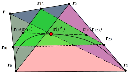
Figure 2: The osculating plane

Secondly, we claim that there exist no $t_{1}^{\star}<t_{2}^{\star}$ in $[t_{0},t_{1}]$ such that the osculating planes $O(t_{1}^{\star})$ and $O(t_{2}^{\star})$ have the same intersection point ${\mathbf{r}}_{01}$ with ${\mathbf{r}}_{0}{\mathbf{r}}_{1}$. It is sufficient to prove that there has no $t^{\star}\in(t_{0},t_{1})$ such that the osculating plane $O(t^{\star})$ passes through ${\mathbf{r}}_{1}$ by assuming $t_{2}^{\star}=t_{1}$ and denote $t_{1}^{\star}$ by $t^{\star}$. Otherwise, if the osculating plane $O(t^{\star})$ passes through ${\mathbf{r}}_{1}$, then $O(t^{\star})$ passes through the line ${\mathbf{r}}_{1}{\mathbf{r}}(t^{\star})$ but cannot pass through ${\mathbf{r}}_{0}$ and ${\mathbf{r}}_{3}$ by the restrictions in condition I). Hence $O(t^{\star})$ has only two possible cases: it either intersects ${\mathbf{r}}_{0}{\mathbf{r}}_{3}$ and the polygonal line ${\mathbf{r}}_{0}{\mathbf{r}}_{2}{\mathbf{r}}_{3}$, or intersects ${\mathbf{r}}_{0}{\mathbf{r}}_{2}$ and ${\mathbf{r}}_{2}{\mathbf{r}}_{3}$. In the first case, let the intersection points of ${\mathbf{T}}(t^{\star})$ and $O(t_{0})$, $O(t_{1})$ be ${\mathbf{r}}_{O_{0}},{\mathbf{r}}_{O_{1}}$ respectively. Then ${\mathbf{r}}_{O_{0}}$ and ${\mathbf{r}}_{O_{1}}$ are on the same side with respect to ${\mathbf{r}}(t^{\star})$ in line ${\mathbf{T}}(t^{\star})$. Which means that one of the sub-segments ${\mathbf{r}}^{\star}_{1}(t),t\in[t_{0},t^{\star}]$ and ${\mathbf{r}}^{\star}_{2}(t),t\in[t^{\star},t_{1}]$ cannot be inside its tetrahedron by the first paragraph of the proof, a contradiction to Proposition 3.7. In the second case, the points ${\mathbf{r}}_{0}$ and ${\mathbf{r}}_{3}$ are on the same side of $O(t^{\star})$. By Proposition 3.7, the sub-segment curves at $t=t^{\star}$ are also on the same side of $O(t^{\star})$. Then the curve ${\mathbf{r}}(t)$ does not pass through $O(t^{\star})$ at $t^{\star}$, which means that $\tau(t^{\star})=0$ by Lemma 3.9. Hence, $\|{\mathbf{r}}_{0}{\mathbf{r}}_{01}\|$ and $\|{\mathbf{r}}_{2}{\mathbf{r}}_{23}\|$ are monotone.

It is known that ${\mathbf{r}}_{01}$ lies on ${\mathbf{r}}_{0}{\mathbf{r}}_{1}$ and ${\mathbf{r}}_{23}$ lies on ${\mathbf{r}}_{2}{\mathbf{r}}_{3}$. We claim that ${\mathbf{r}}_{12}$ must be on ${\mathbf{r}}_{1}{\mathbf{r}}_{2}$. Otherwise, assuming $O(t^{\star})$ has no common points with ${\mathbf{r}}_{1}{\mathbf{r}}_{2}$, then $O(t^{\star})$ must intersect with ${\mathbf{r}}_{0}{\mathbf{r}}_{1},{\mathbf{r}}_{0}{\mathbf{r}}_{2},{\mathbf{r}}_{1}{\mathbf{r}}_{3},$ and ${\mathbf{r}}_{2}{\mathbf{r}}_{3}$. That means ${\mathbf{r}}_{0}$ and ${\mathbf{r}}_{3}$ are on the same side of $O(t^{\star})$, and then $\tau(t^{\star})=0$, a contradiction.

Since the curve is inside its tetrahedron, ${\mathbf{r}}(t^{\star})$ is inside the quadrangle ${\mathbf{r}}_{01}{\mathbf{r}}_{12}{\mathbf{r}}_{23}{\mathbf{r}}_{30}$. Actually, ${\mathbf{r}}(t^{\star})$ is inside the triangle ${\mathbf{r}}_{01}{\mathbf{r}}_{12}{\mathbf{r}}_{23}$. ${\mathbf{r}}(t^{\star})$ cannot be on ${\mathbf{r}}_{01}$ and ${\mathbf{r}}_{23}$ according to condition III). So, if ${\mathbf{r}}(t^{\star})$ is not inside the triangle ${\mathbf{r}}_{01}{\mathbf{r}}_{12}{\mathbf{r}}_{23}$, then ${\mathbf{r}}(t^{\star})$ is on the opposite side with ${\mathbf{r}}_{12}$ with respect to ${\mathbf{r}}_{01}{\mathbf{r}}_{23}$ or on ${\mathbf{r}}_{01}{\mathbf{r}}_{23}$. Then ${\mathbf{T}}(t^{\star})\bigcap O(t_{0})$ is not inside ${\mathbf{r}}_{01}{\mathbf{r}}_{12}$, or, ${\mathbf{T}}(t^{\star})\bigcap O(t_{1})$ is not inside ${\mathbf{r}}_{12}{\mathbf{r}}_{23}$, since ${\mathbf{r}}_{01}{\mathbf{r}}_{12}{\mathbf{r}}_{23}{\mathbf{r}}_{30}$ is convex. Without loss of generality, we suppose ${\mathbf{T}}(t^{\star})\bigcap O(t_{0})$ is not in ${\mathbf{r}}_{01}{\mathbf{r}}_{12}$. Then ${\mathbf{T}}(t^{\star})\bigcap O(t_{0})$ are on the same side with ${\mathbf{r}}_{2}$ w.r.t. ${\mathbf{r}}_{0}{\mathbf{r}}_{1}$ in $O(t_{0})$ by Lemma 3.8. Hence, ${\mathbf{T}}(t^{\star})\bigcap O(t_{0})$ and ${\mathbf{T}}(t^{\star})\bigcap O(t_{1})$ is on the same side of ${\mathbf{r}}(t^{\star})$ in ${\mathbf{T}}(t^{\star})$, which means that one of the sub-segments ${\mathbf{r}}^{\star}_{1}(t),t\in[t_{0},t^{\star}]$ and ${\mathbf{r}}^{\star}_{2}(t),t\in[t^{\star},t_{1}]$ cannot be inside its tetrahedron, a contradiction to Proposition 3.7.

Therefore, ${\mathbf{r}}(t^{\star})$ can only be inside the triangle ${\mathbf{r}}_{01}{\mathbf{r}}_{12}{\mathbf{r}}_{23}$, and ${\mathbf{T}}(t^{\star})$ can only intersect ${\mathbf{r}}_{01}{\mathbf{r}}_{12}$ with ${\mathbf{r}}_{012}$ and intersect ${\mathbf{r}}_{12}{\mathbf{r}}_{23}$ with ${\mathbf{r}}_{123}$. Subdivide ${\mathbf{r}}(t)$ at $t=t^{\star}$ to get curve segments ${\mathbf{r}}_{1}^{\star}(t),t\in[t_{0},t^{\star}]$, and ${\mathbf{r}}_{2}^{\star}(t),t\in[t^{\star},t_{1}]$, and their tetrahedrons as $\lozenge{\mathbf{r}}_{0}{\mathbf{r}}_{01}{\mathbf{r}}_{012}{\mathbf{r}}(t^{\star})$ and $\lozenge{\mathbf{r}}(t^{\star}){\mathbf{r}}_{123}{\mathbf{r}}_{23}{\mathbf{r}}_{3}$. It has been shown that these two sub-tetrahedrons are inside the tetrahedron $\lozenge{\mathbf{r}}_{0}{\mathbf{r}}_{1}{\mathbf{r}}_{2}{\mathbf{r}}_{3}$. As a consequence, for any $t^{\star}_{1}<t^{\star}_{2}$ in $[t_{0},t_{1}]$, the sub-tetrahedron of the sub-segment ${\mathbf{r}}^{\star}(t),t\in[t^{\star}_{1},t^{\star}_{2}]$ is inside the tetrahedron $\lozenge{\mathbf{r}}_{0}{\mathbf{r}}_{1}{\mathbf{r}}_{2}{\mathbf{r}}_{3}$.

Finally, we prove that $\|{\mathbf{r}}_{1}{\mathbf{r}}_{12}\|$ is monotone. It suffices to show that there exist no $t^{\star}_{1}<t^{\star}_{2}\in[t_{0},t_{1}]$ such that $O(t^{\star}_{1})$ and $O(t^{\star}_{2})$ have a common point in ${\mathbf{r}}_{1}{\mathbf{r}}_{2}$. Otherwise, we assume $O(t^{\star}_{1})$ and $O(t^{\star}_{2})$ have a common point ${\mathbf{r}}_{12}^{\star}$ in ${\mathbf{r}}_{1}{\mathbf{r}}_{2}$. Since ${\mathbf{r}}_{0}{\mathbf{r}}_{01}$ and ${\mathbf{r}}_{2}{\mathbf{r}}_{23}$ are monotonously increasing, ${\mathbf{r}}_{01}(t_{1}^{\star})$ and ${\mathbf{r}}_{23}(t_{1}^{\star})$ are on the same side of $O(t_{2}^{\star})$. Hence the intersection line of $O(t^{\star}_{1})$ and $O(t^{\star}_{2})$ can only be outside of the tetrahedron $\lozenge{\mathbf{r}}_{0}{\mathbf{r}}_{1}{\mathbf{r}}_{2}{\mathbf{r}}_{3}$ passing through ${\mathbf{r}}_{12}^{\star}$. Then the sub-tetrahedron of the sub-segment ${\mathbf{r}}^{\star}_{12}(t),t\in[t^{\star}_{1},t^{\star}_{2}]$, cannot be inside the tetrahedron $\lozenge{\mathbf{r}}_{0}{\mathbf{r}}_{1}{\mathbf{r}}_{2}{\mathbf{r}}_{3}$, which contradicts to the consequence in the preceding paragraph.

For clarity, we summarize the properties mentioned in the proof of the above theorem as follows.

Proposition 3.11

For any $t^{\star}_{1}<t^{\star}_{2}\in[t_{0},t_{1}]$, the sub-tetrahedron $\lozenge{\mathbf{r}}_{0}^{\star}{\mathbf{r}}_{1}^{\star}{\mathbf{r}}_{2}^{\star}{\mathbf{r}}_{3}^{\star}$ of the sub-segment ${\mathbf{r}}^{\star}(t),t\in[t^{\star}_{1},t^{\star}_{2}]$ is inside the tetrahedron $\lozenge{\mathbf{r}}_{0}{\mathbf{r}}_{1}{\mathbf{r}}_{2}{\mathbf{r}}_{3}$.

Similar to 7) of Lemma 2.1, we have the following proposition. The proof is also similar to that of 7) of Lemma 2.1.

Proposition 3.12

$\|{\mathbf{r}}_{0}{\mathbf{r}}_{03}\|$ and $\|{\mathbf{r}}_{1}{\mathbf{r}}_{12}\|$ are strictly monotone with $t^{\star}\in(t_{0},t_{1})$ where ${\mathbf{r}}_{03}$ and ${\mathbf{r}}_{12}$ are the intersection points ${\mathbf{r}}_{1}{\mathbf{r}}_{2}{\mathbf{r}}(t^{\star})\bigcap{\mathbf{r}}_{0}{\mathbf{r}}_{3}$ and ${\mathbf{r}}_{0}{\mathbf{r}}_{3}{\mathbf{r}}(t^{\star})\bigcap{\mathbf{r}}_{1}{\mathbf{r}}_{2}$ respectively.

Proof 10

It is sufficient to prove that the planes ${\mathbf{r}}_{1}{\mathbf{r}}_{2}{\mathbf{r}}(t^{\star})$ and ${\mathbf{r}}_{0}{\mathbf{r}}_{3}{\mathbf{r}}(t^{\star})$ are not tangent to ${\mathbf{r}}(t)$ at $t^{\star}\in(t_{0},t_{1})$. If the plane ${\mathbf{r}}_{1}{\mathbf{r}}_{2}{\mathbf{r}}(t^{\star})$ is tangent to ${\mathbf{r}}(t)$ at $t^{\star}\in(t_{0},t_{1})$, then the osculating plane $O(t^{\star})$ must intersect ${\mathbf{r}}_{1}{\mathbf{r}}_{2}{\mathbf{r}}(t^{\star})$ with the tangent line ${\mathbf{T}}(t^{\star})$. By Theorem 3.10, ${\mathbf{T}}(t^{\star})$ must intersect ${\mathbf{r}}_{1}{\mathbf{r}}_{2}$ which is the common line of $O(t_{0})$ and $O(t_{1})$. Dividing the curve segment into two sub-segments ${\mathbf{r}}_{1}^{\star}(t)$ and ${\mathbf{r}}_{2}^{\star}(t)$, then one of them cannot be inside its sub-tetrahedron according to Lemma 3.8 which contradicts to Proposition 3.11. And one can similarly discuss the case for the plane ${\mathbf{r}}_{0}{\mathbf{r}}_{3}{\mathbf{r}}(t^{\star})$.

According to Proposition 3.12, ${\mathbf{r}}(t)$ and the plane ${\mathbf{r}}_{1}{\mathbf{r}}_{2}{\mathbf{r}}_{M}$ have a unique intersection point ${\mathbf{s}}_{\mathbf{r}}$ where ${\mathbf{r}}_{M}=({\mathbf{r}}_{0}+{\mathbf{r}}_{3})/2$. We call ${\mathbf{s}}_{\mathbf{r}}$ the shoulder point of the segment ${\mathbf{r}}(t),t\in[t_{0},t_{1}]$. Similar to Proposition 3.7, we can see that Theorem 3.10 and Proposition 3.12 also hold for any subsegment ${\mathbf{r}}^{\star}(t),t\in[t^{\star}_{1},t^{\star}_{2}]$.

When we subdivide the approximated curve segment at a point $t=t^{\star}$, by Theorem 3.10, we assume that the osculating plane $O(t^{\star})$ intersects ${\mathbf{r}}_{0}{\mathbf{r}}_{1},{\mathbf{r}}_{1}{\mathbf{r}}_{2}$ and ${\mathbf{r}}_{2}{\mathbf{r}}_{3}$ at ${\mathbf{r}}_{01},{\mathbf{r}}_{12}$ and ${\mathbf{r}}_{23}$ respectively. Then, one can have the following corollary.

Corollary 3.13

Let $k_{1}(t^{\star})=\frac{|{\mathbf{r}}_{1}{\mathbf{r}}_{01}|}{|{\mathbf{r}}_{1}{\mathbf{r}}_{0}|},k_{2}(t^{\star})=\frac{|{\mathbf{r}}_{2}{\mathbf{r}}_{12}|}{|{\mathbf{r}}_{2}{\mathbf{r}}_{1}|}$ and $k_{3}(t^{\star})=\frac{|{\mathbf{r}}_{3}{\mathbf{r}}_{23}|}{|{\mathbf{r}}_{3}{\mathbf{r}}_{2}|}$, then $k_{i}(t^{\star})$ is monotone and $k_{i}(t^{\star})\in(0,1)$ with $t^{\star}\in(t_{0},t_{1})$, $i=1,2,3$.

We finally give the Proof of Theorem 3.2 by summarizing the above discussions.

Proof 11

Set $t_{1}$ as Theorem 3.6, then ${\mathbf{r}}(t),t\in[t_{0},t_{1}]$ has the eight properties in Theorem 3.6, 3.10 and Propositions 3.11, 3.12. It means that the segment ${\mathbf{r}}(t),t\in[t_{0},t_{1}]$ is a quasi-cubic segment.

3.3 Subdivision algorithm

As we mentioned in the introduction, the topology graph $\mathcal{G}$ of a parametric space curve can be computed by the method in [27].

A topology graph is a graph $\mathcal{G}=\{{\mathcal{V}},{\mathcal{E}}\}$ where ${\mathcal{V}}$ is a set of points in the Euclidean space ${\mathcal{V}}=\{{\mathbf{v}}_{i}=(\alpha_{i},\beta_{i},\gamma_{i})\}$ and ${\mathcal{E}}$ is a set of edges ${\mathcal{E}}=\{({\mathbf{v}}_{i},{\mathbf{v}}_{j})|{\mathbf{v}}_{i},{\mathbf{v}}_{j}\in{\mathcal{V}}\}$, any two edges do not intersect except in the endpoints. A graph $\mathcal{G}$ is a topology graph of a parametric space curve ${\mathbf{r}}(t)$ if $\mathcal{G}$ and ${\mathbf{r}}(t)$ have the same topology.

The singular points of the space curve are included as vertices in $\mathcal{G}$. In this paper, we need to add more information to the vertices in our algorithm. For each vertex ${\mathbf{v}}_{i}$ in the topology graph, we now update it to

$$V_{i} = \{{\mathbf{v}}_{i}={\mathbf{r}}(t_{i0}),\{t_{i0},t_{i1},\dots,t_{ik}\},$$ (3.4)

$$\{\mathcal{F}_{i0}^{-},\dots,\mathcal{F}_{ik}^{-}\},\{\mathcal{F}_{i0}^{+},\dots,\mathcal{F}_{ik}^{+}\}\},$$

where each $t_{ij}$ is a real parameter such that ${\mathbf{r}}(t_{ij})={\mathbf{v}}_{i}$, $\mathcal{F}_{ij}^{-}$ and $\mathcal{F}_{i0}^{+}$ are the left and right Frenet frames of ${\mathbf{v}}_{i}$ with respect to the parameters $t_{ij},j=0,\ldots,k$. The point set ${\mathcal{V}}$ thus updated is called the extended vertex list. Methods to compute the limitation of the tangent are also introduced in [23].

The edges in $\mathcal{G}$ are not used directly in our approximation algorithm, but they give the connection relationship of two updated vertices. Since the space curve is parametric, the connection relationship is given by the parameters corresponding to the points in ${\mathcal{V}}$ in the increasing order. So in our paper, we use the extended vertex list $\mathcal{V}$ instead of topology graph.

Example 3.14

Figure 3 (a) shows a space curve with a cusp, whose topology graph is given in Figure 3 (b). Figure 4(a) shows a numerical approximate curve which does not pass through the cusp. We may use the topology graph or a refined topology graph to approximate the curve segment as shown in Figure 4(b). This method has two drawbacks. First, we generally needs hundreds even thousands line segments to approximate the curve segment for a small precision [24]. Second, the approximate curve cannot keep the tangent directions of left and right sides of the cusp point. In this paper, we use a cubic Bézier curve instead of a line segment as shown in Figure 4(c), which is not only more precise but keeps the geometric properties of the original curve.

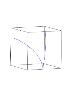
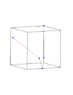
(a) Origin curve                                        (b) Topology graph

Figure 3: Topology graph of the curve

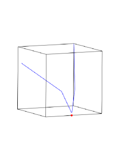
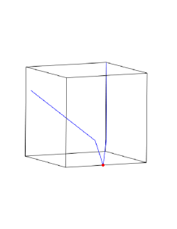
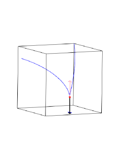
(a) General numerical method               (b) Based on topology                  (c) Proposed method

Figure 4: Numerical approximate curve

Based on the above analysis, we now give the segment dividing algorithm.

Algorithm 3.15

Curve Subdivision.
Input: A normal curve segment ${\mathbf{r}}(t),t\in[0,1]$.
Output: An extended vertex list with elements as (3.4).

1. Compute the certified vertex list $\mathcal{V}$ with all character points as vertices with the method in [27]. The parameters and the left and right Frenet frames are recorded. Suppose the real roots associated to the character points are $s_{i},i=1,\ldots,l-1$ and $0=s_{0}<s_{1}<\cdots<s_{l}=1$.

2. Divide each interval $[s_{i},s_{i+1}]$ as $s_{i}=s_{i0}<s_{i,1}<\cdots<s_{i,k_{i}}=s_{i+1}$ such that each segment satisfies the conditions given in I) to IV).

3. Rearrange the $s_{ij}$ in an ascending order and rename them as $t_{i},i=0,\ldots,n$. Find the left and right Frenet frames of each segment ${\mathbf{r}}(t),t\in[t_{i},t_{i+1}]$.

4. Add all these new points to the extended vertex list $\mathcal{V}$ which is now ready for approximation.

Each curve segment is defined by two adjoint vertices of $\mathcal{V}$. By Proposition 3.7, the curve segment from the algorithm is in the tetrahedron and has the properties in Theorems 3.6, 3.10 and Propositions 3.11, 3.12. Hence each curve segment obtained from Algorithm 3.15 is a quasi-cubic segment and so are its sub-segments.

4 Shoulder point approximation

In this section, we propose an efficient algorithm to construct a set of cubic Bézier curve segments which approximate a quasi-cubic segment obtained in Algorithm 3.15 to any approximate bound.

Firstly, we focus on one quasi-cubic segment ${\mathbf{r}}(t),t\in[t_{0},t_{1}]$. Let ${\mathbf{r}}_{0},{\mathbf{r}}_{3}$ be the endpoints of the segment, ${\mathbf{r}}_{1}$ the intersection point of the tangent line at ${\mathbf{r}}_{0}$ and the osculating plane of ${\mathbf{r}}_{3}$, and ${\mathbf{r}}_{2}$ the intersection point of the tangent line at ${\mathbf{r}}_{3}$ and the osculating plane of ${\mathbf{r}}_{0}$. Then $\{{\mathbf{r}}_{0},{\mathbf{r}}_{1},{\mathbf{r}}_{2},{\mathbf{r}}_{3}\}$ defines a family of rational cubic curves

$${\mathbf{p}}(\omega_{1},\omega_{2},s)=\frac{{\mathbf{r}}_{0}B_{0}(s)+\omega_{1}{\mathbf{r}}_{1}B_{1}(s)+\omega_{2}{\mathbf{r}}_{2}B_{2}(s)+{\mathbf{r}}_{3}B_{3}(s)}{B_{0}(s)+\omega_{1}B_{1}(s)+\omega_{2}B_{2}(s)+B_{3}(s)},\ s\in[0,1].$$ (4.1)

Then ${\mathbf{p}}(\omega_{1},\omega_{2},s)$ is called the associated cubic Bézier curve segment of ${\mathbf{r}}(t)$. It has been shown that ${\mathbf{p}}(\omega_{1},\omega_{2},s)$ meets ${\mathbf{r}}(t)$ at its endpoints ${\mathbf{r}}(t_{0})$ and ${\mathbf{r}}(t_{1})$. Furthermore, ${\mathbf{p}}(\omega_{1},\omega_{2},s)$ and ${\mathbf{r}}(t)$ have the same left and right tangent directions and osculating planes at the endpoints, and the same control tetrahedron $\lozenge{\mathbf{r}}_{0}{\mathbf{r}}_{1}{\mathbf{r}}_{2}{\mathbf{r}}_{3}$.

Proposition 4.1

Let ${\mathbf{p}}(\omega_{1},\omega_{2},s),s\in[0,1]$ be the associated cubic Bézier curve segment of ${\mathbf{r}}(t),t\in[t_{0},t_{1}]$. Then ${\mathbf{p}}(\omega_{1},\omega_{2},s)$ can approximate ${\mathbf{r}}(t)$ at their endpoints with order two by setting proper $\omega_{1}$ and $\omega_{2}$, i.e., $\{{\mathbf{p}}(0)={\mathbf{r}}(t_{0}),{\mathbf{p}}(1)={\mathbf{r}}(t_{1})\}$ and $\{{\mathbf{p}}^{\prime}(0)={\mathbf{r}}^{\prime}(t_{0}),{\mathbf{p}}^{\prime}(1)={\mathbf{r}}^{\prime}(t_{1})\}$.

Proof 12

Following the construction of ${\mathbf{p}}(s)$ for ${\mathbf{r}}(t)$, they are $G^{1}$ interpolated at their endpoints with arbitrary weights $\omega_{1}$ and $\omega_{2}$. According to the properties of the cubic Bézier curve, one can set the proper $\omega_{1}$ and $\omega_{2}$ such that ${\mathbf{p}}(s)$ and ${\mathbf{r}}(t)$ are $C^{1}$ interpolated at their endpoints.

In Proposition 4.1, the weights are selected to enhance the approximation order from $G^{1}$ to $C^{1}$ at the endpoints. Actually, on can get $\{{\mathbf{p}}(\omega_{1},\omega_{2},0)={\mathbf{r}}(t_{0}),{\mathbf{p}}(\omega_{1},\omega_{2},1)={\mathbf{r}}(t_{1})\}$ and $\{{\mathbf{p}}^{\prime}(\omega_{1},\omega_{2},0)=k_{1}\omega_{1}{\mathbf{r}}^{\prime}(t_{0}),{\mathbf{p}}^{\prime}(\omega_{1},\omega_{2},1)=k_{2}\omega_{2}{\mathbf{r}}^{\prime}(t_{1})\}$, where $k_{1}$ and $k_{2}$ are positive constants. Hence we can set $\omega_{1}$ and $\omega_{2}$ such that $k_{1}\omega_{1}=1$ and $k_{2}\omega_{2}=1$. However, in the following paragraphs, we would like to use the freedom of weights to minimize the position approximation error. Hence, we will show how to compute the proper weights $\omega_{1},\omega_{2}$ such that ${\mathbf{p}}(s)$ is an optimal approximation to ${\mathbf{r}}(t)$.

The selection of the weights often leads to some optimization problems such as $\min_{\omega_{1},\omega_{2}}$ $(\max_{s,t}d(\omega_{1},\omega_{2},s,t)^{2})$ where $d(\omega_{1},\omega_{2},s,t)$ is the distance function between ${\mathbf{p}}(\omega_{1},\omega_{2},s)$ and ${\mathbf{r}}(t)$ in certain forms [3]. The computation is usually not efficient and some global error analysis is introduced to simplify the optimization problem [35]. Another possible method is to approximate the target curve segment by checking the parallel points. We can push the parallel points of the approximated curve and the approximate curve (4.1) as near as possible. It also leads to an optimal problem for a function with degree three. In the following, we introduce a novel method which avoids any optimizations.

The shoulder point ${\mathbf{s}}_{\mathbf{p}}$ of ${\mathbf{p}}(s)$ is given in Proposition 2.3. The shoulder point ${\mathbf{s}}_{\mathbf{r}}$ of ${\mathbf{r}}(t)$ can be computed as the unique intersection point of ${\mathbf{r}}(t)$ and the triangle ${\mathbf{r}}_{1}{\mathbf{r}}_{2}{\mathbf{r}}_{M}$. Supposing the plane $P(x,y,z)$ is defined by ${\mathbf{r}}_{1}$, ${\mathbf{r}}_{2}$, and ${\mathbf{r}}_{M}$, then the shoulder point corresponds to a real root $t^{\star}\in(t_{0},t_{1})$ of $P\circ r(t)$ with ${\mathbf{r}}(t^{\star})$ lying in the triangle ${\mathbf{r}}_{1}{\mathbf{r}}_{2}{\mathbf{r}}_{M}$. So $D(\omega_{1},\omega_{2})=\|{\mathbf{s}}_{\mathbf{p}}-{\mathbf{s}}_{\mathbf{r}}\|^{2}$ is a rational function in $\omega_{1},\omega_{2}$ with total degree two. Finding the positive solution from the equations

$$\left\{\begin{array}[]{l}\dfrac{\partial{D}}{\partial\omega_{1}}=0,\\[8.5359pt] \dfrac{\partial{D}}{\partial\omega_{2}}=0,\end{array}\right.$$ (4.2)

we obtain the weights for the approximate cubic curve (4.1).

Before the approximation, we will estimate the error between the two curves. Since there does not have any simple method to compute the distance of two parametric curves with different parameters, we use the distance between ${\mathbf{r}}$ and the implicit variety of a rational cubic curve ${\mathbf{p}}$. It has been proved that the associated implicit ideal $I_{\mathbf{p}}$ of ${\mathbf{p}}$ can be computed using the $\mu$-basis method [31] efficiently:

Lemma 4.2

The associated ideal of ${\mathbf{p}}$ has the form $I_{\mathbf{p}}=\langle f(x,y,z),g(x,y,z)$, $h(x,y,z)\rangle$, where $f,g$ and $h$ are quadratic polynomials, i.e., the resultants of ${\mathbf{p}}^{\prime}s$ $\mu$-basis in pairs.

The algorithm of $\mu$-basis is given in [36]. Generalizing the approximation error function in [37], we have

$$e(f,{\mathbf{r}})=\left(\frac{f({\mathbf{r}})^{2}}{f_{x}({\mathbf{r}})^{2}+f_{y}({\mathbf{r}})^{2}+f_{z}({\mathbf{r}})^{2}}\right)^{1/2}.$$

Let $e({\mathbf{p}},{\mathbf{r}}):=e(f,{\mathbf{r}})+e(g,{\mathbf{r}})+e(h,{\mathbf{r}})=e(t)$ be the univariate error function in $t$. Then the approximation error can be set as the following optimization problem:

$$e=\max_{t_{0}\leq t\leq t_{1}}(e(t)).$$

There are many methods to solve this problem. However, for the efficiency in practice, we often sample $t$ as $t_{i}=\frac{(t_{1}-t_{0})i}{m},i=0,\ldots,m,$ for a proper $m$, say $m=300$, and set the approximate error as $\max(e(t_{i}))$.

The following algorithm is proposed to approximate a quasi-cubic curve segment via shoulder point approximation.

Algorithm 4.3

Shoulder point approximation
Input: A quasi-cubic curve segment ${\mathbf{r}}(t),t\in[t_{0},t_{1}]$ and a positive error bound $\delta$.
Output: A set of cubic Bézier curves which is a $\delta$-approximation for ${\mathbf{r}}(t)$.

1. Construct the associated tetrahedron of ${\mathbf{r}}(t)$ and the rational Bézier cubic curve ${\mathbf{p}}(\omega_{1},\omega_{2},s),s\in[0,1]$ as shown in (4.1).

2. Compute the weights $(\omega_{1},\omega_{2})$ such that $\|{\mathbf{s}}_{\mathbf{p}}-{\mathbf{s}}_{\mathbf{r}}\|$ is as small as possible.

   1. Compute shoulder points ${\mathbf{s}}_{\mathbf{r}}$ and ${\mathbf{s}}_{\mathbf{p}}(\omega_{1},\omega_{2})$ of ${\mathbf{r}}(t)$ and ${\mathbf{p}}(s)$ respectively.

   2. Find a pair of real roots $(\omega_{1},\omega_{2})$ by solving the equation system (4.2).

3. Compute the approximate error $\bar{\delta}=e(t)$. If $\bar{\delta}<\delta$ then output ${\mathbf{p}}(s)$. Otherwise, divide ${\mathbf{r}}(t)$ to two parts on its middle point of arc length and repeat the approximation process for each subsegment.

Example 4.4

A curve segment ${\mathbf{r}}(t),t\in[0,21/32]$ represented by the black curve with degree six is given by Algorithm 3.15 and the approximate cubic Bézier curve is the red dash curve in Figure 5. The weights are $\omega_{1}=\omega_{2}=1$ in the left figure. After executing step 2 of Algorithm 4.3, we have $\omega_{1}=5/11,\omega_{2}=16/31$ in the right figure. The numerical errors are $0.29$ and $0.04$ respectively computed from error function $e(t)$ by setting $m=300$.

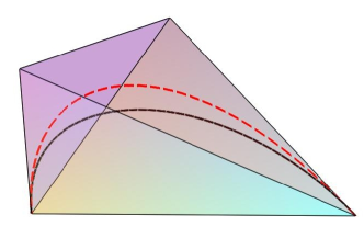
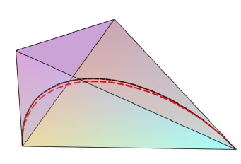
Figure 5: Selecting the weights for Bézier cubic curve

To show the termination of the above algorithm, we need the following lemma.

Lemma 4.5

The edge of the sub-tetrahedron in Algorithm 4.3 converges to zero when the arc length of its subdivided curve segment converges to zero.

Proof 13

There exists a $t=t^{\star}_{1}\in(t_{0},t_{1})$ such that $k_{1}=1/2$ since $k_{1}(t)$ is monotone with $t$ in $(t_{0},t_{1})$ by Corollary 3.13. Consider the subsegment ${\mathbf{r}}(t),t\in[t_{0},t^{\star}_{1}]$ and subdivide it at $t=t^{\star}_{2}$ such that $k_{2}=1/2$ for the sub-tetrahedron $\lozenge(t_{0},t^{\star}_{1})$. Then, subdivide ${\mathbf{r}}(t),t\in[t_{0},t^{\star}_{2}]$ at $t=t^{\star}_{3}$ such that $k_{3}=1/2$ for $\lozenge(t_{0},t^{\star}_{3})$. Let $t^{(1)}=t^{\star}_{3}$. We obtain a subsegment ${\mathbf{r}}(t),t\in[t_{0},t^{(1)}]$ whose sub-tetrahedron $\lozenge(t_{0},t^{(1)})$ has vertices ${\mathbf{r}}_{0}^{(1)}={\mathbf{r}}_{0},{\mathbf{r}}_{1}^{(1)},{\mathbf{r}}_{2}^{(1)},{\mathbf{r}}_{3}^{(1)}$. Similarly, we can construct ${\mathbf{r}}_{j}^{(i)},j=0,1,2,3$ and $t^{(i)}$. According to the subdividing process, let ${\mathbf{r}}_{j}^{(0)}={\mathbf{r}}_{j},j=0,1,2,3$. Then, we have $\|{\mathbf{r}}_{0}^{(i)}{\mathbf{r}}_{1}^{(i)}\|<\|{\mathbf{r}}_{0}^{(i-1)}{\mathbf{r}}_{1}^{(i-1)}\|/2$, $\|{\mathbf{r}}_{1}^{(i)}{\mathbf{r}}_{2}^{(i)}\|<\|{\mathbf{r}}_{0}^{(i-1)}{\mathbf{r}}_{1}^{(i-1)}\|/2+\|{\mathbf{r}}_{1}^{(i-1)}{\mathbf{r}}_{2}^{(i-1)}\|/2$ and $\|{\mathbf{r}}_{2}^{(i)}{\mathbf{r}}_{3}^{(i)}\|<\|{\mathbf{r}}_{0}^{(i-1)}{\mathbf{r}}_{1}^{(i-1)}\|/2+\|{\mathbf{r}}_{1}^{(i-1)}{\mathbf{r}}_{2}^{(i-1)}\|+\|{\mathbf{r}}_{2}^{(i-1)}{\mathbf{r}}_{3}^{(i-1)}\|/2$ for $i>0$. Hence, the lengthes of the three edges $\|{\mathbf{r}}_{0}^{(i)}{\mathbf{r}}_{1}^{(i)}\|$, $\|{\mathbf{r}}_{1}^{(i)}{\mathbf{r}}_{2}^{(i)}\|$ and $\|{\mathbf{r}}_{2}^{(i)}{\mathbf{r}}_{3}^{(i)}\|$ of a sub-tetrahedron $\lozenge(t_{0},t^{(i)})$ converge to zero when $i\rightarrow\infty$. Since ${\mathbf{r}}(t),t\in[t_{0},t_{1}]$ is a rational curve and has no singular point, $t^{(i)}-t_{0}$ converges to zero when $i\rightarrow\infty$.

Let $t\in[t_{0},t_{1}]$ and $\lozenge{\mathbf{r}}_{0}{\mathbf{r}}_{1}^{\prime}(t){\mathbf{r}}_{2}^{\prime}(t){\mathbf{r}}_{3}^{\prime}(t)$ its tetrahedron. Then $s(t)=\|{\mathbf{r}}_{0}{\mathbf{r}}_{1}^{\prime}(t)\|+\|{\mathbf{r}}_{1}^{\prime}(t){\mathbf{r}}_{2}^{\prime}(t)\|+\|{\mathbf{r}}_{2}^{\prime}(t){\mathbf{r}}_{3}^{\prime}(t)\|$ converges to zero when $t\rightarrow t_{0}$, since ${\mathbf{r}}(t)$ has no singularities in $[t_{0},t_{1}]$. Hence when the arc length of its subdivided curve segment converges to zero, which means $t\rightarrow t_{0}$, the edge of sub-tetrahedron converges to zero.

The termination of Algorithm 4.3 can be guaranteed by the following theorem.

Theorem 4.6

In Algorithm 4.3, the approximation error converges to zero for the subdivision procedure.

Proof 14

By Lemma 4.5, when the arc length of its subdivided curve segment converges to zero, the edge of the sub-tetrahedron converges to zero. Since the approximation error is controlled by the edges, it converges to zero for the subdivision procedure.

Remark 4.7

In Algorithm 4.3, the Step 3 is given to simplify the proof of the convergence. In fact, for less computation, we always implement the algorithm with the following step instead of $3$.

1. Compute the approximate error $\bar{\delta}=e(t)$. If $\bar{\delta}<\delta$ then output ${\mathbf{p}}(s)$. Otherwise, divide ${\mathbf{r}}(t)$ to two parts on its shoulder point ${\mathbf{s}}_{\mathbf{r}}$ repeat the approximation process for each subsegment.

According to the proof of Lemma 4.5, the algorithm fails if a subsequence of $s_{i}$ does not converge to zero under shoulder point subdivision process, and it never happened in our experiments. It is an interesting problem to prove the termination of this version of the algorithm.

5 Algorithms and experimental results

After dividing the curve to segments by Algorithm 3.15, we can approximate each curve segment by the shoulder approximation method in Algorithm 4.3. In this section, we give the main approximation algorithm and the experimental results.

The global approximation is based on the local approximation and topology determination in the above sections. Some relationships of the approximate curve segments are considerable in the global view. In our approximation, the line edges in the topology graph are replaced by the associated cubic Bézier curve segments. To ensure the topological isotopy before and after the replacement, we restrict the cubic curve segments to have the appropriate topology based on the topology graph.

It is shown that an associated cubic Bézier curve segment are decided by its tetrahedron. Let $\lozenge{\mathbf{p}}_{0}^{1}{\mathbf{p}}_{1}^{1}{\mathbf{p}}_{2}^{1}{\mathbf{p}}_{3}^{1}$ and $\lozenge{\mathbf{p}}_{0}^{2}{\mathbf{p}}_{1}^{2}{\mathbf{p}}_{2}^{2}{\mathbf{p}}_{3}^{2}$ be two control tetrahedrons of two cubic Bézier curve segments ${\mathbf{p}}^{1}(s)$ and ${\mathbf{p}}^{2}(s)$. Then ${\mathbf{p}}^{1}(s)$ and ${\mathbf{p}}^{2}(s)$ can have no common points except for their endpoints. In the further consideration, we give two cases for the problem. The first case is that ${\mathbf{p}}^{1}(s)$ and ${\mathbf{p}}^{2}(s)$ have only one common point being the endpoint and the same Frenet frames at this endpoint. And the other positional situations of ${\mathbf{p}}^{1}(s)$ and ${\mathbf{p}}^{2}(s)$ are included in the second case.

If all the pairs of cubic Bézier curves satisfy the second case, then to ensure that cubic curve segment does not bring in the unexpected knots while it replaces the line edge, one can give a sufficient condition that each cubic curve segment has no common points with the control tetrahedron of another curve segment except for the endpoint. This condition can be strengthened if we do not want to check the collision between a cubic curve segment and a tetrahedron. The condition can be that the two tetrahedrons have no inner points. By Lemma 4.5, the condition can be satisfied by subdividing the curve segments. Then the approximate curve have same topology with the given curve, since the approximate curve is controlled by the sequence of the tetrahedrons. Each tetrahedron has no common inner points with other tetrahedrons.

We then only need to discuss the pairs of cubic Bézier curves belong to the first case. Assuming ${\mathbf{p}}_{0}^{1}={\mathbf{p}}_{0}^{2}$, then ${\mathbf{p}}_{1}^{2}$ is on the radial $(1-\lambda){\mathbf{p}}_{0}^{1}+\lambda{\mathbf{p}}_{1}^{1},\lambda\geq 0$, and ${\mathbf{p}}_{2}^{2}$ is on the same side with ${\mathbf{p}}_{2}^{1}$ on the plane ${\mathbf{p}}_{0}^{1}{\mathbf{p}}_{1}^{1}{\mathbf{p}}_{2}^{1}$. According to the monotonicity of the Bézier curve in Lemma 2.1, ${\mathbf{p}}^{1}(s)$ and ${\mathbf{p}}^{2}(s)$ can replace the their associated line edges without topology modification.

Algorithm 5.1

Certified B-spline approximation with error bound.
Input: A normal curve segment ${\mathbf{r}}(t),t\in[t_{0},t_{1}]$ and a positive error bound ${\delta}$.
Output: A cubic B-spline ${\mathbf{p}}(s)$ such that the approximate error between ${\mathbf{p}}(s)$ and ${\mathbf{r}}(t)$ is less than ${\delta}$ and the approximate implicit spline for ${\mathbf{r}}(t)$.

1. Divide the curve ${\mathbf{r}}(t)$ into quasi-cubic segments by Algorithm 3.15.

2. Check the topology conditions.

   1. Check the intersection of any pair of cubic Bézier curves which have the same Frenet frame at the endpoint, divide them to two parts on their shoulder points respectively, if they have common points more the endpoints.

   2. Check the collision of any pair of tetrahedrons, divide them to two parts on their shoulder points respectively, if they have inner points.

3. For each segment, find the cubic Bézier curves which approximate the given curve segment with precision ${\delta}$ by Algorithm 4.3.

4. Find the implicit form for the cubic Bézier curves with the $\mu$-basis method [31].

5. Convert the resulting rational cubic Bézier curves to a rational B-spline with a proper knot selection as the method presented in [2].

Remark 5.2

In the process of topology conditions checking, we only need to check the collision of the sub-tetrahedrons subdivided from which are the intersected before the subdivision, since the sub-tetrahedrons are included in its father tetrahedrons. It means that the less and less pairs of tetrahedrons need to be checked in the subdivision process.

Theorem 5.3

From Algorithm 5.1, we obtain a piecewise $C^{1}$ continuous approximate cubic B-spline curve which keeps the singular points, inflection points, and torsion vanishing points of the approximated parametric curve. At cusps, the approximate curve is $C^{0}$ continuous.

Proof 15

Algorithm 5.1 gives the $G^{1}$ cubic Bézier spline since it is constructed as the hermite interpolation of the original curve, if the character points are not cusps. Then $C^{1}$ continuity can be ensured from the conversion from the Bézier spline with a proper knot selection [2]. The singular points of the curve are treated as segmenting points. Since at the segmenting points, the left and right Frenet frames are preserved, the origin curve and the approximate curve have the same singular points. Since the cubic spline introduces no more singular points, the algorithm keeps the singular points. At a cusp, its left (right) tangent and osculating plane are kept according to Algorithm 3.15, and the approximate curve is then only $C^{0}$ continuous.

The character points include the vertices of the topology graph. The topology conditions ensure that the topology is persevered while the topolgy line edges are replaced by the cubic Bézier curve segments. According to Theorem 4.6, the approximate curve from Algorithm 5.1 converges to the approximated curve and they have the same topology.

The left and right Frenet frames of the approximate curves are the same as that of the approximated curve at the character points, which means that the principal normal vector and the osculating plane are both kept. Then the principal normal vector changes its direction at the inflection point. Similarly, the curve does not pass through the osculating plane at the torsion vanishing point.

Finally, we give several examples to illustrate the algorithm.

Example 5.4

The space curve ${\mathbf{r}}_{1}(t)$ from Example 6 in [27] has a singular point $(0,0,0)$ at $t=\pm 1,\pm\infty$, where

$${\mathbf{r}}_{1}(t)=\left({\frac{1-t^{2}}{\left(t^{2}+1\right)^{2}}},{\frac{t\left(1-t^{2}\right)}{\left(t^{2}+1\right)^{2}}},{\frac{t^{2}\left(1-t^{2}\right)}{\left(t^{2}+1\right)^{4}}}\right).$$

The curve segment ${\mathbf{r}}_{1}(t),t\in[-2,2]$ and its approximate spline curve ${\mathbf{p}}(s)$ are shown in Figure 6, they are shown in the same figure for comparison and the tetrahedron sequence is also given in Figure 7, the numerical error $e(t)$ is shown in Figure 8.

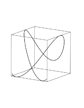
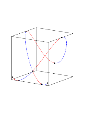
Figure 6: ${\mathbf{r}}_{1}(t)$ and ${\mathbf{p}}(s)$

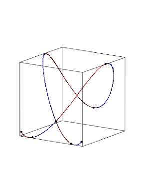
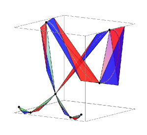
Figure 7: ${\mathbf{r}}_{1}(t)$ v.s. ${\mathbf{p}}(s)$ and control tetrahedron

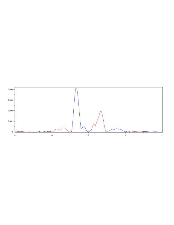
Figure 8: Numerical error for ${\mathbf{r}}_{1}$ with $m=300$

As we know, the point $(0,0,0)$ is a characteristic point from the topology determining. It is preserved in ${\mathbf{p}}(s)$ and ${\mathbf{p}}(s)$ is $C^{1}$ at this point. Each corresponding segment of ${\mathbf{p}}(s)$ and ${\mathbf{r}}_{1}(t)$ is interpolated with the Frenet Frames at the endpoints. One can find that ${\mathbf{r}}_{1}(t),t\in[-\infty,+\infty]$ is an asymmetric space trifolium curve. To approximate the other two parts of $t\in[-\infty,-2]$ and $t\in[2,+\infty]$, we can transform $t=\pm\infty$ to $t=0$ by a reparametrization as $t^{\prime}=1/t$. Then approximating ${\mathbf{r}}_{1}(t^{\prime}),t^{\prime}\in[-1/2,1/2]$ and combining the former spline segment, we can get the approximation of the whole trifolium curve.

Example 5.5

Two more space curves are given in this example. ${\mathbf{r}}_{2}(t)$ has a complex singular point and ${\mathbf{r}}_{3}(t)$ is a random curve with degree nine.

$${\mathbf{r}}_{2}(t)=\left({\frac{{t}^{2}\left(t-1\right)^{2}}{\left(1+{t}^{2}\right)^{2}}},{\frac{t\left(t-1\right)^{3}}{1+{t}^{2}}},{\frac{t\left(t-1\right)^{4}}{1+{t}^{2}}}.\right),t\in[-1/16,3/2]$$

$$\begin{array}[]{lcl}{\mathbf{r}}_{3}(t)&=&\left({\frac{t\left(1181\,{t}^{8}-1878\,{t}^{7}-1236\,{t}^{6}+1960\,{t}^{5}+2058\,{t}^{4}-2688\,{t}^{3}+532\,{t}^{2}-9+72\,t\right)}{-2+9\,t-72\,{t}^{2}+308\,{t}^{3}-840\,{t}^{4}+1218\,{t}^{5}-952\,{t}^{6}+588\,{t}^{7}-408\,{t}^{8}+149\,{t}^{9}}},\right.\\ &&-{\frac{t\left(-1686\,{t}^{7}+287\,{t}^{8}+3252\,{t}^{6}-2464\,{t}^{5}+462\,{t}^{4}+168\,{t}^{3}-28\,{t}^{2}+9\right)}{-2+9\,t-72\,{t}^{2}+308\,{t}^{3}-840\,{t}^{4}+1218\,{t}^{5}-952\,{t}^{6}+588\,{t}^{7}-408\,{t}^{8}+149\,{t}^{9}}},\\ &&\left.-\,{\frac{4{t}^{2}\left(263\,{t}^{7}-924\,{t}^{6}+1338\,{t}^{5}-1190\,{t}^{4}+861\,{t}^{3}-483\,{t}^{2}+154\,t-18\right)}{-2+9\,t-72\,{t}^{2}+308\,{t}^{3}-840\,{t}^{4}+1218\,{t}^{5}-952\,{t}^{6}+588\,{t}^{7}-408\,{t}^{8}+149\,{t}^{9}}}\right),t\in[0,1]\end{array}$$

The approximated curves, approximate spline curves, and the numerical errors are shown in the following figures (Figures 9, 10, 11). In ${\mathbf{r}}_{2}(t)$, $(0,0,0)$ is a self-intersected point with $t=0,1$, it is also a cusp point at $t=1$. This point is preserved in our approximate B-spline curve ${\mathbf{p}}(s)$. Furthermore, the limited tangent directions of the cusp are also preserved. ${\mathbf{p}}(s)$ is $C^{1}$ or $C^{0}$ at $(0,0,0)$ when ${\mathbf{p}}(s)$ passes through $(0,0,0)$ as a self-intersected or a cusp point respectively. The approximation information for curves ${\mathbf{r}}_{1},{\mathbf{r}}_{2}$, and ${\mathbf{r}}_{3}$ is listed in Table 1.

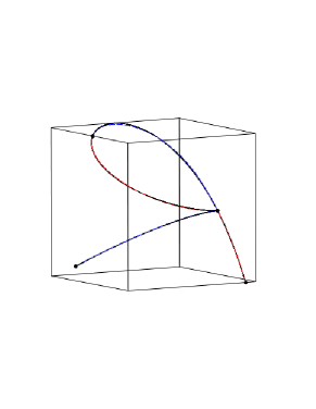
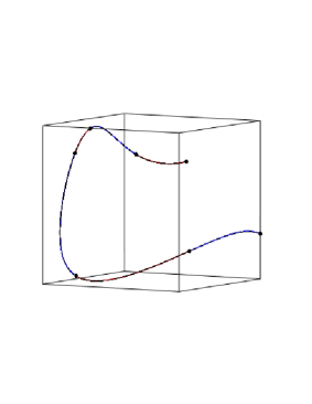
Figure 9: ${\mathbf{r}}_{2}(t)$ v.s. ${\mathbf{p}}_{2}(s)$ and ${\mathbf{r}}_{3}(t)$ v.s. ${\mathbf{p}}_{3}(s)$

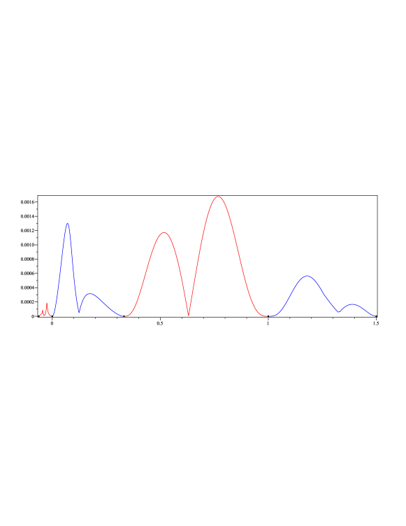
Figure 10: Numerical error for ${\mathbf{r}}_{2}$

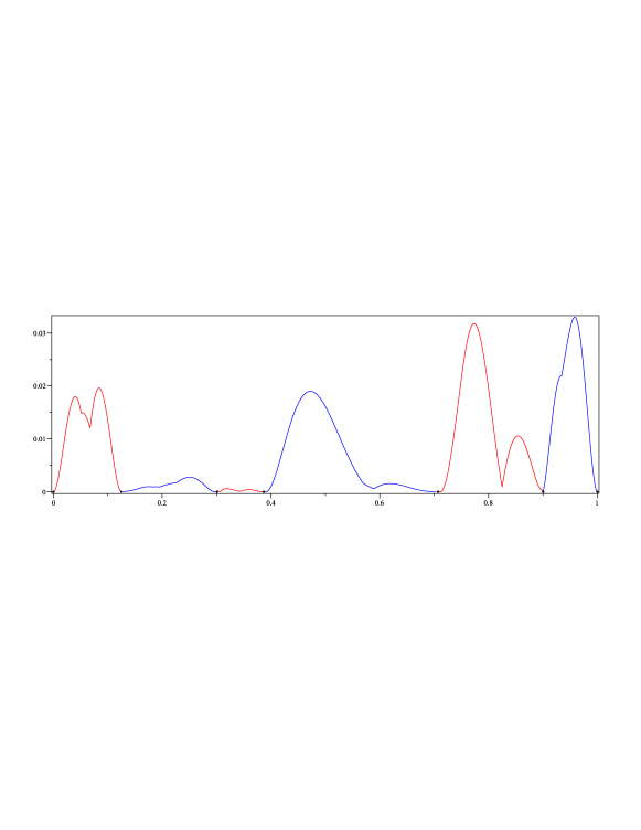
Figure 11: Numerical error for ${\mathbf{r}}_{3}$

curve	degree	error	segments	interval
${\mathbf{r}}_{1}$	$8$	$0.004157$	$8$	$[-2,2]$
${\mathbf{r}}_{2}$	$5$	$0.0001677$	$4$	$[-\frac{1}{16},\frac{3}{2}]$
${\mathbf{r}}_{3}$	$9$	$0.03298$	$6$	$[0,1]$

Table 1: Numerical Approximation

6 Conclusion and further work

We present an algorithm to construct a rational cubic B-spline approximation for a space parametric curve. The main purpose of the work is to present an isotopic approximation method which preserves the geometric features of the original curve. The approximated curve is divided into quasi-cubic segments which have similar properties to those of a cubic Bézier curve. Sufficient conditions are proposed for a divided segment having the expected properties and then its approximate Bézier spline is naturally constructed. Based on these properties, the shoulder point approximate algorithm is presented and it is proved to be convergent. An approximate implicitization can be found by the $\mu$-basis method. The method is applicable for any parametric space curve in theory, although the given conditions are more difficult to compute when the parametric expression is not in rational form.

The intersection curve of a parametric surface and an implicit surface is another important type of space curves. The curve can be regarded as parametric form with two parameters and a constraint function for them. As a further work, we will study the approximation of this type of space curve.

References

- Hoschek and Lasser [1993] J. Hoschek, D. Lasser, Fundamentals of computer aided geometric design, A. K. Peters, Ltd., Natick, MA, USA, translator-Schumaker, Larry L., 1993.
- Piegl and Tiller [1997] L. Piegl, W. Tiller, The NURBS book (2nd ed.), Springer-Verlag New York, Inc., New York, NY, USA, 1997.
- Pottmann et al. [2002] H. Pottmann, S. Leopoldseder, M. Hofer, Approximation with Active B-Spline Curves and Surfaces, in: PG ’02: Proceedings of the 10th Pacific Conference on Computer Graphics and Applications, 8, 2002.
- Renka [2005] R. J. Renka, Shape-preserving interpolation by fair discrete space curves, Comput. Aided Geom. Des. Vol.22 (No.8) (2005) 793–809.
- Aigner et al. [2007] M. Aigner, Z. Šír, B. Jüttler, Evolution-based least-squares fitting using Pythagorean hodograph spline curves, Comput. Aided Geom. Des. Vol.24 (2007) 310–322.
- Kong and Ong [2009] V. P. Kong, B. H. Ong, Shape preserving approximation by spatial cubic splines, Comput. Aided Geom. Des. Vol.26 (No.8) (2009) 888–903.
- Degen [1993] W. L. F. Degen, High accurate rational approximation of parametric curves, Comput. Aided Geom. Des. Vol.10 (No.3-4) (1993) 293–313.
- Degen [2005] W. L. F. Degen, Geometric Hermite interpolation: in memoriam Josef Hoschek , Comput. Aided Geom. Des. Vol.22 (No.7) (2005) 573–592.
- Farin [2008] G. Farin, Geometric Hermite interpolation with circular precision, Computer-Aided Design Vol.40 (No.4) (2008) 476–479.
- Hijllig and Koch [1995] K. Hijllig, J. Koch, Geometric Hermite interpolation, Comput. Aided Geom. Des. Vol.12 (No.6) (1995) 567–580.
- Xu and Shi [2005] L. Xu, J. Shi, Geometric Hermite interpolation for space curves, Comput. Aided Geom. Des. Vol.18 (No.9) (2001) 817–829.
- Pelosi et al. [2005] F. Pelosi, R.T. Farouki, C. Manni, A. Sestini, Geometric Hermite interpolation by spatial Pythagorean-hodograph cubics, Advances in Computational Mathematics Vol.22 (2005) 325–352.
- Rababah [2007] A. Rababah, High accuracy Hermite approximation for space curves in , Journal of Mathematical Analysis and Applications Vol.325 (No.2) (2007) 920–931.
- Chen et al. [2010] X.D. Chen, W. Ma, J.C. Paul, Cubic B-spline curve approximation by curve unclamping , Computer-Aided Design Vol.42 (No.6) (2010) 523–534.
- Gao and Li [2004] X.S. Gao, M. Li, Rational quadratic approximation to real algebraic curves, Comput. Aided Geom. Des. Vol.21 (No.8) (2004) 805–828.
- Yang [2004] X. Yang, Curve fitting and fairing using conic splines, Computer-Aided Design Vol.36 (No.5) (2004) 461 – 472.
- Li et al. [2006] M. Li, X.S. Gao, S.C. Chou, Quadratic approximation to plane parametric curves and its application in approximate implicitization, Vis. Comput. Vol.22 (No.9) (2006) 906–917.
- Ghosh et al. [2007] S. Ghosh, S. Petitjean, G. Vegter, Approximation by Conic Splines, Mathematics in Computer Science Vol.1 (2007) 39–69.
- Zhongke et al. [2003] Z.K. Wu, F. Lin, S. H. Soon, Topology preserving voxelisation of rational Bézier and NURBS curves, Computers & Graphics Vol.27 (No.1) (2003) 83–89.
- Chen et al. [2011] Y. Chen, L.Y. Shen, C.M. Yuan, Collision and intersection detection of two ruled surfaces using bracket method, Comput. Aided Geom. Des. Vol.28 (No.2) (2011) 114–126.
- Alcázar and Sendra [2005] J. G. Alcázar, J. R. Sendra, Computation of the topology of real algebraic space curves, Journal of Symbolic Computation Vol.39 (No.6) (2005) 719–744.
- Liang et al. [2009] C. Liang, B. Mourrain, J.P. Pavone, Subdivision Methods for the Topology of 2d and 3d Implicit Curves, in: Geometric Modeling and Algebraic Geometry, 199–214, 2009.
- Daouda et al. [2008] D. N. Daouda, B. Mourrain, O. Ruatta, On the computation of the topology of a non-reduced implicit space curve, in: ISSAC ’08: Proceedings of the twenty-first international symposium on Symbolic and algebraic computation, 47–54, 2008.
- Cheng et al. [2009b] J.S. Cheng, X.S. Gao, J. Li, Topology determination and isolation for implicit plane curves, in: Proc. ACM Symposium on Applied Computing, 1140–1141, 2009b.
- Wang et al. [2009] H. Wang, X. Jia, R. Goldman, Axial moving planes and singularities of rational space curves, Comput. Aided Geom. Des. Vol.26 (No.3) (2009) 300–316.
- Rubio et al. [2009] R. Rubio, J. M. Serradilla, M. P. Vélez, Detecting real singularities of a space curve from a real rational parametrization, J. Symb. Comput. Vol.44 (No.5) (2009) 490–498.
- Alcázar and Díaz-Toca [2010] J. G. Alcázar, G. M. Díaz-Toca, Topology of 2D and 3D rational curves, Comput. Aided Geom. Des. Vol.27 (No.7) (2010) 483–502.
- Forrest [1980] A. Forrest, The twisted cubic curve: a computer-aided geometric design approach, Computer-Aided Design Vol.12 (No.4) (1980) 165–172.
- Chen et al. [2002] J. Chen, S. Zhang, H. Bao, Q. Peng, continuous curve modeling with rational cubic Bézier spline, Process in Natural Science Vol.12 (2002) 217–221.
- Manocha and Canny [1992] D. Manocha, J. F. Canny, Detecting cusps and inflection points in curves, Comput. Aided Geom. Des. Vol.9 (No.1) (1992) 1–24.
- Cox et al. [1998] D. A. Cox, T. W. Sederberg, F. Chen, The moving line ideal basis of planar rational curves, Comput. Aided Geom. Des. Vol.15 (No.8) (1998) 803–827.
- Li and Cripps [1997] Y.M. Li, R. J. Cripps, Identification of inflection points and cusps on rational curves, Computer Aided Geometric Design Vol.14 (No.5) (1997) 491 – 497.
- Rouillier and Zimmermann [2004] F. Rouillier, P. Zimmermann, Efficient isolation of polynomial’s real roots, J. Comput. Appl. Math. Vol.162 (No.1) (2004) 33–50.
- Cheng et al. [2009a] J.S. Cheng, X.S. Gao, C.-K. Yap, Complete numerical isolation of real roots in zero-dimensional triangular systems, Journal of Symbolic Computation Vol.44 (No.7) (2009a) 768–785.
- Dokken [2001] T. Dokken, Approximate implicitization, in: Mathematical Methods for Curves and Surfaces: Oslo 2000, 81–102, 2001.
- Deng et al. [2005] J. Deng, F. Chen, L.Y. Shen, Computing -bases of rational curves and surfaces using polynomial matrix factorization, in: ISSAC ’05: Proceedings of the 2005 international symposium on Symbolic and algebraic computation, 132–139, 2005.
- Chuang and Hoffmann [1989] J. H. Chuang, C. M. Hoffmann, On local implicit approximation and its applications, ACM Trans. Graph. Vol.8 (No.4) (1989) 298–324.