In light of upcoming observations modelling perturbations in dark energy and modified gravity models has become an important topic of research. We develop an effective action to construct the components of the perturbed dark energy momentum tensor which appears in the perturbed generalized gravitational field equations, for linearized perturbations. Our method does not require knowledge of the Lagrangian density of the dark sector to be provided, only its field content. The method is based on the fact that it is only necessary to specify the perturbed Lagrangian to quadratic order and couples this with the assumption of global statistical isotropy of spatial sections to show that the model can be specified completely in terms of a finite number of background dependent functions. We present our formalism in a coordinate independent fashion and provide explicit formulae for the perturbed conservation equation and the components of for two explicit generic examples: (i) the dark sector does not contain extra fields, and (ii) the dark sector contains a scalar field and its first derivative . We discuss how the formalism can be applied to modified gravity models containing derivatives of the metric, curvature tensors, higher derivatives of the scalar fields and vector fields.
1 Introduction
The standard model of cosmology uses General Relativity (GR) to describe gravitational interactions, an homogeneous/isotropic FRW metric to describe the geometry and matter content of cold dark matter (CDM)/photons/baryons to describe its constituents. Observations of the cosmic microwave background, supernovae, baryon acoustic oscillations, gravitational lensing and structure formation point to the existence of an additional component dubbed “dark energy”, or a modification to gravity, which needs to be introduced to explain the the observed acceleration 1933AcHPh…6..110Z ; Riess:1998cb ; Perlmutter:1998np ; Riess:1998dv ; 0067-0049-192-2-18 .
The simplest explanation is a cosmological constant, , and the standard paradigm is the CDM model. However, there is still considerable flexibility for the explanation to be something radically different. In general, we can model all possible theories as an extra “dark sector” component to the stress-energy-momentum tensor. The structure of the gravitational field equations means that this extra component can be used to model either “exotic matter” with an equation of state or a modification to GR (i.e. modifying exactly how gravity responds to the presence of matter). Constructing viable models of modified gravity has become an important task with the discovery of the acceleration of the Universe; some modified gravity models may also be able to account for observations which otherwise require dark matter.
In this paper we describe a new way of parameterizing perturbations in the dark sector requiring as an assumption knowledge of the field content. We do not assume a specific Lagrangian density, but we are able to model the possible effects on observations by using an effective action to compute the possible perturbations to the gravitational field equations. This is done by limiting the action to terms which are quadratic in the perturbed field content which is sufficient to model linearized perturbations, and assuming that the spatial sections are isotropic. In this paper we only consider the case that the dark sector contains first order derivatives of scalar fields and the metric; we will discuss higher order derivatives and vector fields in a follow-up paper.
Our theories will be completely general allowing for all possible degrees of freedom. Initially we do not impose reparametrization, or gauge, invariance. This is something which we would expect of a fundamental theory of dark energy, but not necessarily one for which the field content is just a coarse grained description. We will find that this can lead to an phenomological vector degree of freedom, . In the elastic dark energy theory Battye:2005mm ; Battye:2006mb ; PhysRevD.76.023005 ; Battye:2009ze , which can be used to describe the effects of a dark energy component composed of a topological defect lattice, this represents a perturbation of the elastic medium from its equilibrium. We will see that the imposition of reparametrization invariance substantially reduces the number of free functions.
We note that many authors have consider possible dark energy theories which are effective Lagrangians in the traditional sense, that is, the terms in the Lagrangian represent an expansion of field operators which are suppressed at low energies Weinberg:2008hq ; Cheung:2007st ; Creminelli:2008wc . Our approach here is sufficiently similar to this approach to share the epitaph “effective action”, but it is completely different in many ways. It is completely classical and is in no sense an expansion energy scale. Moreover, it is just an effective action for the perturbations, and in no sense represents the full field theory of the dark energy.
2 Approaches to parameterizing dark sector perturbations
In this section we will provide a brief review of current approaches to studying generalized gravitational theories, concluding with a short discussion on the generalities of our approach.
2.1 Parameterized post-Friedmannian approach
A popular way to parameterize the dark sector takes an “observational” perspective. One can modify the equations governing the predictions of the Newtonian gravitational potential and shear by introducing extra functions space and time into the relevant equations and then parametrizing these extra functions in an ad hoc fashion. Since it is possible to explicitly observe and via the evolution structure and gravitational shear PhysRevD.69.083503 ; PhysRevD.76.023507 ; PhysRevD.81.083534 ; PhysRevD.81.104023 ; Hojjati:2011ix (see also the more recent papers Dossett:2011tn ; Kirk:2011sw ; Laszlo:2011sv ), one can then compare them with the predictions of particular ad hoc choice and determine constraints on the deviation of a particular parameter from its value in General Relativity.
One way of doing this is by modifying the Poisson and gravitational slip equations, introducing two scale- and time-dependent functions, and . The Poisson and gravitational-slip equations then become
(1)
where is the comoving density perturbation, the density contrast, the velocity divergence field, the equation of state and is the anisotropic stress. When these equations are derived in GR one finds that , and so if, by comparison to data, either of these parameters are shown to be inconsistent with unity, then deviations from GR can be established. In Baker:2011jy ; Zuntz:2011aq it was shown that the two functions are not necessarily independent: they can be linked by the perturbed Bianchi identity, depending on the structure of the underlying theory.
2.2 Generalized gravitational field equations
Another way to investigate the dark sector takes a more theoretical standpoint, and is based on a more consistent modification of the governing field equations. The method stems from the fact that any modified gravity theory or model of dark energy can be encapsulated by writing the generalized gravitational field equations
(2)
where is the Einstein tensor calculated from the spacetime metric, is the energy-momentum tensor of all known species (radiation, Baryons, CDM etc) and is a tensor which contains all unknown contributions to the gravitational field equations, which we call the dark energy-momentum tensorPhysRevD.76.104043 ; PhysRevD.77.103524 ; PhysRevD.79.123527 .
Because the Bianchi identity automatically holds for the Einstein tensor, , in the standard case where the known and unknown sectors are decoupled (that is ) we have the conservation law
(3)
This represents a constraint equation on the extra parameters and functions that may appear in a parameterization of the dark sector at the level of the background. At perturbed order, the parameterization of is constrained by the perturbed conservation law
(4)
The shortcoming of this approach is that one must supply the components of . Skordis PhysRevD.79.123527 does this by expanding the components in terms of pseudo derivative operators acting upon gauge invariant combinations of metric perturbations, by imposing the principles that (a) the field equations remain at most second order and (b) the equations are gauge-form invariant. A particular form of these components were considered in PhysRevD.79.123527 :
(5a)
(5b)
where is a set of pseudo differential operators and are gauge invariant combinations of perturbed metric variables. The possible form that the elements of can take is constrained by the perturbed Bianchi identity. For instance, it was shown that is one of the sufficient consistency relations. A generalized version of this method can be found in Baker:2011jy ; Clifton:2011jh .
This scheme provides a way to compute and constrain observables without ever having to write down an explicit theory for the dark sector. There appears to be, however, a weakness in the current formulation of this strategy: there does not seem to be a physically obvious way to interpret the ; for example, if one were to find that is “required” for consistency with observational data, what does that impose physically upon the system? It is exactly this issue we address in this paper.
2.3 Effective action approach
The generalized gravitational field equations (2) can be constructed from an action
(6)
The matter Lagrangian density contains all known matter fields (e.g. baryons, photons) and is used to construct the known energy momentum tensor , and the dark sector Lagrangian density contains all “unknown” contributions to the gravitational sector, and will be used to construct the dark energy momentum tensor . One can define
(7)
The dark sector Lagrangian may contain known fields in an unknown configuration or extra fields, but of course we do not know a priori what the dark sector Lagrangian density is.
Two simple cases are (i) a slowly-rolling minimally coupled scalar field parameterized by a potential, , and (ii) a modified gravity model parameterized by a free function of the Ricci scalar, . There are restrictions on the form of both of these functions to achieve acceleration, but once they have been applied there is still considerable freedom in the choices of and and wide ranges of behaviour of the expansion history, , can be arranged for particular choices of the functions. One would expect this to be the case in any self consistent dark energy model compatible with FRW metric and therefore it might seen reasonable to make the assumption that the dark stress-energy-momentum tensor where is in 1-1 correspondence with . The important question, which we are concerned with, is how to parametrize the perturbations in a general way based on some general physical principle. In this way our approach is similar to that discussed in section 2.2
The overall ethos which we advocate is to write down an effective action, inspired by the approach that is taken in particle physics (see, e.g. PhysRevD.8.1226 ) where, for example, the most general modifications to the standard model are written down for a given field content that are compatible with some assumed symmetry/symmetries. Then all the free coefficients are constrained by experiment. In our case, we will specify the field content of the dark sector, for example, scalar or vector fields, and write down a general quadratic Lagrangian density for the perturbed field variables which is sufficient to generate equations of motion for linearized perturbations. We will also make the assumption that the spatial sections are isotropic which substantially reduces the number of free coefficients.
3 Formalism
3.1 Second order Lagrangian
The underlying principle behind our method is to write down a effective Lagrangian density for perturbed field variables. If our theory is constructed from a set of field variables , then we write each field variable as a linearized perturbation about some background value,
(8)
The action for the perturbed field variables is computed by integrating a Lagrangian density which is quadratic in the perturbed field variables. If there are “N” perturbed field variables, the effective Lagrangian density for the perturbed field variables is given by
(9)
where is a set of arbitrary functions only depending on the background field variables; clearly, . To obtain the equation of motion of the perturbed field variables we must induce some variation in the and subsequently demand that is independent of these variations. If we vary the perturbed field variables with a variational operator ,
(10)
then the effective Lagrangian will vary according to ,
where
(11)
The demand that the effective Lagrangian is independent of these variations is the statement that
(12)
that is,
(13)
These equations provide the equations of motion of the perturbed field variables. We will now show how to obtain the effective action for perturbations by directly perturbing the background action.
We will consider an action of the form
(14)
where is the determinant of the spacetime metric, , and is the Lagrangian density, which contains all fields in the theory. It will be useful to write the first and second variations of the action as
We will only consider first perturbations of the field content of a theory.
For the action (14) we can use the well known result
(17)
to show that to quadratic order in the perturbations that the integrands in (15) are given by
(18a)
(18b)
We treat the integrand of the second variation of the action, i.e. , as the effective Lagrangian, , for linearized perturbations, and it is called the second order Lagrangian. The final term of (18b) is an effective mass-term for the gravitational fluctuations which is always present even when the field which constitutes the dark sector does not vary, i.e. when .
Although we will be providing various explicit examples later on in the paper, we will briefly discuss how to write down once the field content has been specified. If the field content is , then we write , and then is written down by writing all quadratic interactions of the perturbed fields with appropriate coefficients,
(19)
Notice that we have moved from having complete ignorance of how the fields combine to construct the Lagrangian density to only requiring 3 “background” functions, to be able to write down. Typically, we would expect these functions to be specified in terms of the scale factor .
The theories we consider contribute to the gravitational field equations via the dark energy-momentum tensor, , which we define in the usual way, (7).
The indices on the dark energy momentum tensor are symmetric by construction,
(20)
where tensor indices are symmetrised as . The dark energy-momentum tensor above can be directly perturbed to give
(21)
where are the perturbed field variables. This can be written in a more succinct way by using the second order Lagrangian,
(22)
Therefore, to obtain the gravitational contribution at perturbed order, due to our effective Lagrangian for perturbed field variables, one must compute the derivative of the second order Lagrangian with respect to the perturbed metric.
The equations of motion for a field and its perturbation are found by regarding and as the relevant Lagrangian densities. Explicitly, the equations of motion for the field and its perturbation, , are respectively given by
(23)
The equations of motion governing the perturbation to the metric, , are given by the perturbed gravitational field equations,
(24)
The perturbed conservation law for the dark energy-momentum tensor is
(25)
which can be written as
(26)
3.2 Isotropic (3+1) decomposition
We will impose isotropy of spatial sections on the background spacetime. The motivation for doing this is that our goal is to study perturbations about an FRW background. After imposing isotropy we are able to use an isotropic (3+1) decomposition to significantly simplify expressions. It is also possible to include anisotropic backgrounds as described in Battye:2006mb .
We will foliate the 4D spacetime by 3D surfaces orthogonal to a time-like vector , which is normalized via
(27)
This induces an embedding of a 3D surface in a 4D space. The 4D metric is and the 3D metric is , and they are related by
(28)
The foliation implies that the time-like vector is orthogonal to the 3D metric,
(29)
The foliation induces a symmetric extrinsic curvature, , which is entirely spatial, . We can use this to deduce that .
A common application of the (3+1) decomposition is to write down the only energy-momentum tensor compatible with the globally isotropic FRW metric,
(30)
There are only two “coefficients” used in the decomposition of the energy-momentum tensor: the energy-density and pressure ,
(31)
Writing a tensor as a sum over combinations of and defines the isotropic (3+1) decomposition. We will now show how to decompose tensors of higher rank. For example, an isotropic vector is completely decomposed as
(32)
where . Notice that before we imposed isotropy upon we would need 4 functions to specify all “free” components of ; by imposing isotropy we have reduced the number of “free” functions from . A symmetric rank-2 isotropic tensor is completely decomposed as
(33)
where .
The time-like part of is and the space-like part is . A rank-3 tensor symmetric in its second two indices is completely decomposed as
(34)
This formalism can also be used to construct tensors which are entirely spatial. For example, a rank-4 tensor defined as
(35)
is entirely spatial, a fact which is manifested by , after one notes the symmetries in the indices .
The coefficients which appear in an isotropic decomposition can only have time-like derivatives. For the coefficients in (33) we have
(36)
where an overdot is used to denote differentiation in the direction of the time-like vector: .
A quantity is perturbed about a background value, , as . For example, the metric perturbed about a background is written as
(37)
It is important to realize that the operation of index raising and lowering does not commute with the variation. For example,
for the metric and for the derivative of a scalar field .
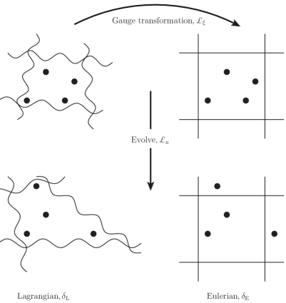
Consider a quantity which is perturbed about some background value, . We can then employ two classes of coordinate system to follow the perturbation through evolution; time evolution can be thought of as Lie-dragging a quantity along a time-like vector, , to “carve out” the world-line of the perturbation, i.e. operating on a quantity with . The first is where the density of the perturbations remains fixed (i.e. the coordinate system evolves to comove with the perturbations); this is a Lagrangian system. In the second, the coordinate system is fixed by some means (such as knowledge of the background geometry) and the density of the perturbations changes; this is an Eulerian system. We write perturbations in the Lagrangian system as and perturbations in the Eulerian system as . Evidently, a coordinate transformation can be used to transfer between the two systems, . The Eulerian and Lagrangian variations are linked by
(38)
where is the Lie derivative along the gauge field . This setup is schematically depicted in Figure 1.
Figure 1: Schematic view of the Eulerian and Lagrangian coordinate systems. The Lagrangian system can be said to be comoving, and the Eulerian system as being fixed. The Lagrangian system retains the density of a field, whereas the Eulerian system does not. This is schematically depicted by the “grid square” becoming deformed in the Lagrangian system on the left, to accommodate the movement of “particles” upon evolution in time. The grid square in the Eulerian system has remained fixed, meaning that the number of particles in a given square changes upon evolution. In cosmology we are perturbing against a fixed background: the FRW background, however calculations are often easier to perform in a comoving system. This means that physical relevance is taken from equations perturbed according to a Eulerian scheme.
Without loss of generality we can set the gauge field and time-like vector to be mutually orthogonal,
(39)
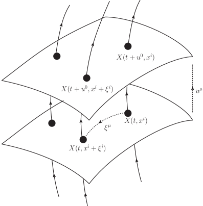
This is because the time-like transformations which the component could induce are world-line preserving, and are redundant when is present (which is inherently a world-line preserving evolution). See Figure 2 for a schematic view illustrating this point.
Figure 2: Schematic view of the foliation and evolution, with three example world-lines drawn on, each piercing two 3D surfaces; is a time-like vector satisfying . A quantity on a surface with spacetime location can be transformed into a quantity on the same surface but at a different location by transforming the coordinate on the surface, . This is a diffeomorphism which drags one world-line into another. If the time coordinate is transformed then the quantity is evaluated on a different 3d surface, but on the same world-line. Thus, if we were to have a transformation , where is an arbitrary scalar field, the time-like part of is redundant. Hence, we are free to set , fixing the time-like part of the diffeomorphism field to be zero. So, we should have the interpretation that moves between world-lines and moves along world-lines.
There is an important question which arises: which perturbation scheme should we use to derive cosmologically relevant results, i.e. which should we use: or ? In cosmological perturbation theory a quantity is perturbed from its value in a fixed (or known) background (such as its value in an FRW background). Therefore, equations should be perturbed relative to a fixed background, and so we should employ the Eulerian scheme.
The equation of motion governing the metric perturbations is
(40)
and the perturbed conservation law that should be solved is the one evaluated in a Eulerian system,
(41)
which can be written as
(42)
If the Lagrangian variation of the dark energy-momentum tensor is the quantity that is supplied, (i.e. is given), then one must be careful to use (38), to obtain the Eulerian perturbed quantity,
(43)
Furthermore, to obtain the components of the mixed Eulerian perturbed dark energy-momentum tensor, one must use
(44)
The Lagrangian and Eulerian perturbations of the metric are linked by
(45)
For a vector field one finds that
(46)
As final explicit example, the Eulerian and Lagrangian variations of a scalar field are linked via
(47)
An interesting lemma is that if then by (39) we find that the Eulerian and Lagrangian variations of a scalar field are identical, . This means that a diffeomorphism does not change the perturbations of the scalar field; this is a consequence of the background field being homogeneous.
4 No extra fields:
Our first and simplest example is where the dark sector does not contain any extra fields: only the metric is present, albeit in an arbitrary combination. This class of theories contains the cosmological constant and elastic dark energy PhysRevD.60.043505 ; PhysRevD.76.023005 , and will also include more general theories that have not been previously considered. In this section we do not allow the dark sector to contain derivatives of the metric – this is discussed in a subsequent section. One of the aims is to build an intuition for understanding how to write down perturbative quantities and how to decompose tensors which arise in the perturbative equations.
The Lagrangian density we will consider in this section is of the form
(48)
so that the second order Lagrangian is given by
(49)
The rank-4 tensor is only a function of background quantities, and is therefore manifestly gauge invariant.
We can use (22) and (49) to show that the perturbations to the dark energy momentum tensor are given by
(50)
By inspecting (49) it follows that the tensor enjoys the following symmetries,
(51)
This shows us how to construct the Lagrangian perturbations to the generalized gravitational field equations, under the assumption that the dark sector Lagrangian is a function of the metric only. Because it is the Lagrangian variation which appears above we must convert to Eulerian variations to obtain cosmologically relevant perturbations. By using (45) and (43) in (50) we obtain
To find the equation of motion of the vector field, , we must compute the Eulerian perturbed Bianchi identity. Substituting (4) into (42) we obtain
(53a)
where, for convenience, we have defined
(53b)
and where the perturbed source term, , is given by
(53c)
Here we observe that the metric perturbations and the diffeomorphism field are intimately linked: one cannot consistently set either to zero.
The equation (53) is the constraint equation for any parameters/functions that appear in a parameterization of the dark sector, under the rather general assumption that ; the only freedom that remains is how to construct out of background quantities. In Section 6 we will provide the components of the equation of motion for a perturbed FRW spacetime.
The only way to write the tensors with an isotropic (3+1) decomposition which respects the symmetries (51) is
(54a)
(54b)
where respects the same symmetries as , satisfies (i.e. is entirely spatial) and is given by
(54c)
A concrete example of a theory which only contains the metric is the elastic dark energy theory PhysRevD.60.043505 ; PhysRevD.76.023005 where one can find that the coefficients in terms of physical quantities such as energy density , pressure , bulk and shear moduli are given by
(55a)
(55b)
where the bulk modulus is defined via , and the pressure and shear modulus are functions of the density (e.g. one way to choose these functional dependancies is with an “equation of state”, and , so that ).
In this section we have identified that just five functions are required to specify the perturbations in the dark sector when no extra fields are present. These five functions are
(56)
and each function only depends on background quantities and are governed by the background evolution.
5 Scalar fields:
The second example is when the dark sector contains an arbitrary combination of scalar field , the first derivative of the field , and the metric . This encompasses scalar field theories such as quintessence and -essence, but we could also encompass a range of other possible theories.
For a Lagrangian density given by
(57)
the second order Lagrangian is given by
(58)
The coefficients above comprise: one scalar , one vector , two rank-2 tensors , one rank-3 tensor, and one rank-4 tensor , all of which are only functions of background quantities and are therefore gauge invariant. At first sight these are all independent quantities, but we will show later that the conservation and Euler-Lagrange equations can be used to link the quantities. By inspecting (58) these tensors enjoy the following symmetries,
(59a)
(59b)
In what follows we will assume (alternatively this can be stated as ), so that . This is the covariant statement that is entirely time-like, while using the fact that the diffeomorphism is entirely space-like. Therefore, because the Eulerian and Lagrangian perturbations of a scalar field are identical we will not distinguish between them and we will write .
The equation of motion of the perturbed scalar field, , is given by the Euler-Lagrange equation (23). Using (58) one finds
(60)
where the “perturbed source” piece, , is given by
(61)
where .
We note that plays the role of an “effective metric”, due to its resemblance to the corresponding term in the perturbed Klein-Gordon equation, namely , and there is also an effective mass of the -field, .
The isotropic (3+1) decomposition of the coefficients , whilst respecting the symmetries (59), is
(62a)
(62b)
(62c)
(62d)
(62e)
The decompositions of are identical to those given in eq.(54).
Only the terms in (58) which involve are relevant for writing down the perturbations to the dark energy-momentum tensor. We obtain
(63)
The Eulerian perturbed conservation law (42) can be computed using (63). We obtain
(64)
where is given by (53c), and represents the wave equation for and is given by
(65)
Equation (64) is an evolution equation for the scalar field perturbation , sourced by the metric perturbations, , and the vector field, . The scalar field perturbation sources the equation of motion for ,(40), via the components . In general one cannot consistently solve the evolution equations for independently from those for the vector field ; we will soon show how these two fields might decouple, but the decoupling only occurs in special cases.
The perturbed Euler-Lagrange equation (60) and perturbed conservation law (64) are both evolution equations for , and both have apparently different coefficients, resulting in an over-determined system.
We can choose to remove this apparent over-determination by “forcing” the time-like (i.e. scalar) part of the perturbed conservation law to be identical to the perturbed Euler-Lagrange equation. It is important to realize that the perturbed conservation law is a vector equation, and only one of its components can be set equal to the perturbed Euler-Lagrange equation; the other components of the vector equation will introduce a set of constraint equations.
When we contract the perturbed Bianchi identity with a time-like vector (where ), we can read off a set of conditions that link the coefficients appearing in the Euler-Lagrange equation (60) and the perturbed Bianchi identity (64). Doing this we obtain the linking conditions
(66a)
(66b)
(66c)
(66d)
We see, therefore, that the coefficients and that appear in (58) are not independent, which is now obvious from (66).
By differentiating (66a) and comparing with (66b) one finds that
(67)
where is the induced extrinsic curvature and an overdot is used to denote differentiation along the time-like vector.
The (3+1) decomposition introduces some interesting structure and can be used to explicitly evaluate the linking conditions (66). From (66a) we find that
(68)
After combining (66a) and (66b) to yield (67) we find that
One can think of as being an “artificial” vector field whose role was to restore reparameterization invariance, and it would therefore be desirable to have a theory that does not require to be present and reparameterization invariance is manifest. We will derive conditions that the tensors in the Lagrangian must satisfy in order for reparameterization invariance to be manifest.
We can rewrite the Lagrangian with the vector field explicitly present to show how the three fields interact and how the parameters can be arranged so that they ultimately decouple. To ease our calculation we will write , We use (45) to replace with in the Lagrangian (58). Rearranging, whilst keeping track of total derivatives yields
(71)
To enable us to identify the “free” and “interaction” Lagrangians, we note that (71) can be written schematically as
(72)
where of a single field variable represents the self-interaction of that field and of two fields represents the interaction between the two fields.
The final line of (71) is a pure surface term, and will not contribute to the dynamics, and thus does not require consideration in what we are about to discuss. However, if we note the definition of and compare to the perturbed EMT (63), we find that .
Notice that the perturbed scalar field, , and vector field are coupled in the Lagrangian, and only decouple when their interaction Lagrangian, , vanishes. This will remove the direct coupling but they may remain indirectly coupled if the interaction Lagrangian for the perturbed metric and vector field remains non-zero (i.e. if ), since the perturbed metric and scalar field will remain coupled, . So, the interaction Lagrangian between the vector field and perturbed scalar field vanishes, i.e. , when
(73)
For arbitrary values of the perturbed scalar field and vector field, this is satisfied by the covariant conditions
(74)
To find the decoupling conditions for the perturbed metric we realize that because ,
(75)
is an identity. If we contract (64) with and use (73) then
(76)
where and are given respectively by (53c) and (65).
Inserting these definitions of into (76) yields
(77)
For arbitrary values of , the decoupling of from occurs when the coefficients of vanish, which occurs when the covariant conditions
(78)
are satisfied.
Inserting the (3+1) decomposition into (74) and (78) allows us to evaluate the decoupling conditions. This yields
(79a)
(79b)
(79c)
Note that (79c) gives us no information since .
Hence, we conclude that the decoupling conditions (79, 80) are satisfied by the parameter choices
(81a)
(81b)
(81c)
When (81b) is used the first condition of (81c) becomes
(82)
and the second is satisfied identically.
The process of identifying the time-like part of the perturbed conservation law with the Euler-Lagrange equation has reduced the number of functions required to specify from . The eleven functions are
(83)
as well as the energy density and pressure of the dark sector “fluid”. Imposing reparameterization invariance as well, these eleven functions reduce to just five:
(84)
Later on we will show that does not affect the cosmological dynamics, and becomes irrelevant in the synchronous gauge. This means that there are just three free functions left to completely specify the dark sector perturbations for a reparameterization-invaraiant scalar field theory.
In Appendix A we provide the explicit calculation for computing and in a kinetic scalar field theory , where is the kinetic term of a scalar field. In Table 1 we give a summary of the functions that appear in the decomposition of for some explicit scalar field theories; in these examples it is natural to see that upon specifying a scalar field theory the time evolution of the various functions is set. For a canonical scalar field theory, , the functions are given by
(85a)
(85b)
(85c)
(85d)
where an overdot is understood to denote differentiation with respect to time and . Using (85) and taking it transpires that (67) is the Klein-Gordon equation.
Function
(a) EDE
(b)
(c)
(d)
0
0
Table 1: Collection of the functions in the decomposition of . The theories we have presented are: (a) elastic dark energy, (b) generic kinetic scalar field theory, (c) -essence and (d) canonical scalar field theory. It is interesting to realize that the theories with are subsets of theories with . Comma denotes partial differentiation (e.g. ), prime denotes differentiation with respect the functions single argument: , and an overdot denotes differentiation with respect to time; for conformal time coefficients one should replace . The free function does not appear in the decomposition of , but for the sake of completeness its value in an -theory is and in the cases (c, d), .
6 Cosmological perturbations
In this section we provide explicit expressions for the components of and the perturbed conservation equation specialized to the case of an FRW background. We will pay special attention to the scalar field theory, where we will show how the vector field decouples from the equation of motion for .
We will perturb the line element about a conformally flat FRW background, and write
(86)
This means that we are setting the components of the Eulerian perturbed metric to
(87)
The time-like vector is given by , and we set . All functions (83) are only functions of time. The background conservation equation becomes
(88)
where an overdot denotes derivative with respect to conformal time and is the conformal time Hubble parameter. The components of for the theory with field content , (63), are given by
(89a)
(89b)
(89c)
(89d)
These are the sources to the equations governing the evolution of the metric perturbations, and can be used to obtain the components of in the conformal Newtonian and synchronous gauges.
We will now work in the synchronous gauge (by setting ), and we will study the more general theory , which will trivially encompass the no-extra-fields case. The components become
(90a)
(90b)
(90c)
The components of the Eulerian perturbed conservation law , (64), has a “scalar” component and a “vector” component. The component of the perturbed conservation law (64) yields
(91a)
and the component yields
(91b)
We observe that the “scalar” piece (91) of the perturbed conservation law represents the evolution equation for the perturbed scalar field sourced by metric perturbations and the vector field, and the “vector” piece (91) constitutes an evolution equation for the vector field, sourced by the perturbed scalar field and metric perturbations. Notice that nine functions are required to be specified to be able to write down the components and the perturbed conservation law: , (note that do not enter into these quantities).
We will now study the conditions under which and decouple; this will represent a simpler subset of theories, and will provide us with another understanding how the decoupling conditions come about. It is useful to write the perturbed conservation equation (91) as
(92a)
(92b)
where the sets of coefficients can be read off from (91). The and decouple when all common terms in (92) vanish. This yields the conditions and . The former decoupling condition yields
(93a)
(93b)
and the latter decoupling condition yields
(93c)
(93d)
We also require that
(93e)
for decoupling to occur in the . Combining (93a, 93c, 93e) yields the conservation equation: . These conditions are compatible with those we derived covariantly, (81).
Applying the decoupling conditions (93) to the components (90) we obtain
(94a)
(94b)
and to the perturbed conservation equation (91) we obtain
(95)
We now observe that only three functions are required to be specified: . When the decoupling conditions are satisfied, one can consistently set and reparameterization invariance is enforced. The theory is now equivalent to the theory studied in Creminelli:2008wc , where reparameterization invariance was imposed from the implicitly.
6.1 No extra fields
For the theory with no extra fields, we can obtain the components of and those of the perturbed conservation law by ignoring all terms with in (90) and (91) respectively.
The components become
(96a)
(96b)
(96c)
The component of the perturbed conservation law becomes
(97)
and the component of the perturbed conservation law yields
(98)
We can use (6.1) to obtain a set of conditions that enforces the constraint (6.1) on the component of the perturbed conservation equation. We set the coefficients of to zero and obtain
(99a)
(99b)
Applying these conditions to the components of (96) we find
Hence, we see that after applying the conditions (99) there are only two free coefficients which describe perturbations in the dark sector: and .
Making the choice which defines elastic dark energy, (55), one finds that (6.1) agrees with the equation of motion for given in PhysRevD.76.023005 .
6.2 Scalar fields
As an explicit example, we can construct a theory where and enter the field content by combining into the kinetic scalar , so that the field content is . In Table 1 we supplied the coefficients for this general kinetic scalar field theory. The decoupling conditions (93b, 93c) are trivially satisfied, the condition (93a) becomes
which is the Euler-Lagrange equation that one can compute directly and therefore vanishes identically. What this means is that for all scalar field theories of the form , the and fields decouple (i.e. one can set consistently). The components of the perturbed dark energy-momentum tensor become
(104a)
(104b)
The -component of the perturbed conservation law (91) becomes
(105)
which is the evolution equation for the perturbed scalar field (we have verified that this reproduces known results) and only three functions are required to be specified: , in addition to the equation of state, .
7 Generalized perturbed fluid equations
Here we study parameterizations of the generalized perturbed fluid equations. The main point of this section is to identify the entropy contribution, , and anisotropic stresses, , for the generalized dark theories we have discussed in this paper which will allow us to make connections with observations, and to deduce whether or not the form of suggested by Weller:2003hw ; PhysRevD.69.083503 is the most general way in which entropy should be specified. We will continue to work in the synchronous gauge.
In Ma:1995ey ; PhysRevD.76.023005 the perturbed Bianchi identity, , is given for scalar perturbations in the synchronous gauge,
(106a)
(106b)
where is the equation of state , is the density contrast, is the scalar anisotropic source, and the entropy contribution is given by
(107)
where for simplicity we have assumed constant . If the entropy and anisotropic stress can be specified in terms of the perturbed metric and fluid variables,
(108)
then the fluid equations (106) become closed. The expressions (108) constitute equations of state for dark sector perturbations.
In Weller:2003hw ; PhysRevD.69.083503 the fluid equations (106) are modified by introducing a gauge invariant density contrast. Their modification is equivalent to parameterizing the entropy as
(109)
The important thing to notice here is that there is a single function which specifies the entropy: the sound speed . One should note that when the entropy contribution becomes .
It is standard practice to decompose the perturbed energy-momentum tensor with a density perturbation , velocity perturbation , pressure perturbation and anisotropic stresses ,
(110)
The tensor is traceless, so that
(111)
This last expression is a useful way to determine the transverse-traceless components of a tensor.
The scalar decomposition of the gauge field and metric perturbation is
(112a)
where is a transverse-traceless spatial derivative operator, is the spatial Laplacian; the trace of the metric perturbation is and the transverse-traceless part of the metric perturbation is
(112b)
The scalar decomposition of the perturbed fluid variables is
(112c)
We have that is the scalar anisotropic perturbation, and is the scalar velocity divergence perturbation. We will also decompose the vector and tensor pieces of vectorial and tensorial quantities in the usual way; the equations for the vector and tensor sectors are given in PhysRevD.76.023005 . To summarise our decompositions:
(113a)
(113b)
As a final piece of notation, we will extract some of the time dependance of a quantity by dividing out the density and write
(114)
A common example of this is using an equation of state to link the pressure and density, . We will not a priori assume that these “hatted” quantities are constant, but it may well turn out that the problem significantly simplifies if this is the case.
7.1 No extra fields
For the theory with field content , one can use (96) to obtain the perturbed fluid variables
(115a)
(115b)
(115c)
(115d)
(115e)
(115f)
(115g)
The entropy contribution (107) can be identified as
(116)
where we defined
(117)
Hence, we observe that this theory is capable of supporting non-trivial scalar, vector and tensor anisotropic and velocity sources. When one makes the parameter choice corresponding to elastic dark energy (55) one obtains , which is in concordance with the results in PhysRevD.76.023005 .
7.2 Scalar fields
For a theory with field content , one can use (90) to obtain the perturbed fluid variables
(118a)
(118b)
(118c)
(118d)
(118e)
(118f)
(118g)
One should notice that this theory is capable of supporting anisotropic stresses, with in general.
where we have defined three frequently appearing ratios,
(120)
and the combination,
(121)
If we now apply the decoupling conditions (93) to (118, 119, 120), then we find
(122a)
(122b)
(122c)
(122d)
(122e)
where
(123)
One should note that the anisotropic stress has now vanished. The perturbed fluid variables for theories with are special cases of (122). The expressions (122d, 122e) are examples of equations of state for dark sector perturbations.
7.3 Example scalar field theories
There are a number of explicit scalar field theories we will explicitly study which will enable us to get a feel for the typical form of the functions which appear in the entropy. The theories we consider have Lagrangian densities given by
It is interesting to note that two of the frequently appearing combinations are
(130)
which are the logarithmic slopes of and respectively and bear a resemblance to “slow-roll” parameters.
For a pure -essence theory, , we have that and thus from (129) notice that the entropy becomes , which bears a strong resemblance to the form of the entropy in the no extra fields case (116), but it is not of the form suggested by Weller:2003hw ; PhysRevD.69.083503 .
It is possible to construct a Lagrangian density which has a specific equation of state. If we impose upon (125c) then after trivial rearrangement we obtain
(131)
which can be integrated, yielding
(132)
where appears as a “constant of integration”.
We can further impose , perform the integral, and find
(133)
This theory has been constructed to have an equation of state which is independent of the kinetic term. In this case one is able to deduce that
(134)
which means that the entropy for this particular theory vanishes.
7.4 Generalized parameterization of entropy contributions
Motivated by our results in the previous subsections, we write down an expression for the parameterization of , which have been derived from the second order Lagrangian, and which we believe represents a wider range of theories than the parameterization of Weller:2003hw ; PhysRevD.69.083503 . Our parameterization for the entropy contribution is
(135)
where and are both a priori time-dependant background quantities which we have explicitly determined for the no extra fields and scalar field theories, although the hope would be that they would only be slowly varying functions of time. We reiterate that (135) constitutes an equation of state of dark sector perturbations. In Table 2 we provide explicit formulae for these quantities for generic example theories. It should be noted that in the parameterization of Weller:2003hw ; PhysRevD.69.083503 -essence is excluded, and the parameter is always taken to be constant. It is rather simple to determine whether or not can be expected to be constant or not for particular examples, as we show below.
Explicitly, for the theory one obtains
(136)
We have written to isolate a parameter combination, .
For the theory , one obtains
which is the same as (136) but with an extra factor in the expression for .
Table 2: Collection of the quantities which determine the entropy contribution; the function is defined in (117); in the final line we give the parameterization of Weller:2003hw ; PhysRevD.69.083503 .
8 Modified gravity
We will briefly discuss a class of theories which are more obviously “modified gravity” theories: we allow the dark sector to contain derivatives of the metric and no extra scalar fields. The simplest example is where the dark sectors field content is just the metric and its first derivative,
(138)
The second order Lagrangian is given by
The tensors have the symmetries
(140)
(141)
(142)
This construction encompasses models which are often studied in the context of massive gravity theories (see e.g. the reviews Rubakov:2008nh ; Hinterbichler:2011tt ). Explicitly computing the second measure-weighted variation of the Ricci scalar for metric perturbations about an arbitrary background yields
(143)
This formula is clearly of the same form as (8), but with , and reproduces the relevant formulae in Battye:2004se for gravitational perturbations in a Minkowski background, and in Hinterbichler:2011tt for perturbations in a Universe with constant curvature.
Following the usual procedure, the perturbed dark energy-momentum tensor can be computed from (8) and written as
(144)
where is a derivative operator which we write as
(145)
where one can identify
(146a)
(146b)
(146c)
A generic modified gravity theory containing curvature tensors is constructed from a field content
(147)
where is the Riemann tensor. The second order Lagrangian will have the schematic form
(148)
where we have suppressed all indices for ease.
This field content will encompass theories containing arbitrary combinations of the Ricci tensor and scalar, and the Einstein tensor; popular examples of these types of theories include Gauss-Bonnet PhysRevD.67.024030 ; Clifton:2011jh and gravities Capozziello:2003tk ; PhysRevD.70.043528 . To actually compute is rather complicated and technical; we present some important steps in Appendix B and the explicit form of for gravities. We find that the perturbed dark energy-momentum tensor can be written as
(149)
where is a derivative operator which we write as
(150)
We will not present the explicit form of the coefficients in generality in the decomposition of because they are cumbersome and not particularly illuminating at this stage; however, in Appendix B we provide the explicit coefficients for an theory. The coefficients can be written with an isotropic (3+1) decomposition to obtain all the parameters required.
We have only sketched how our formalism can be applied to theories containing high-order derivatives of the metric. However, it is clear that our formalism can be used to write down an effective Lagrangian density for the gravitational fluctuations which will automatically contain entire classes of known theories as well as encompassing theories which have never been considered before. As alluded to above, the second order Lagrangian (143) perhaps represents provide a fruitful theoretical testing ground for massive gravity theories.
9 Discussion
In this paper we have outlined an approach to computing consistent perturbations to the generalized gravitational field equations for physically meaningful theories. The method requires a field content, but does not require a particular Lagrangian density to be presented for calculations to be performed. Once the field content has been specified we have shown how to write down an effective action for linearized perturbations. We imposed isotropy of the spatial sections so that all results we derived are compatible with an FRW metric.
We have provided an argument for why we use the Eulerian coordinate system to construct the perturbations which correspond to physically relevant quantities. The reason is that quantities in cosmology are perturbed about some known background, which is the same as the statement of using the Eulerian perturbation scheme.
We have given two detailed examples illustrating how to use our formalism: one where the field content of the dark sector is entirely composed of the metric, and one where the dark sector contains a scalar field, its derivatives and the metric. A priori we did not constrain these fields to combine into scalar quantities (such as a kinetic term). We gave formulae for the effective Lagrangian for perturbations in these examples, which enabled us to write down the perturbed dark energy momentum tensor, . These expressions involved a number of coefficient-tensors which can be split with an isotropic (3+1) decomposition; the number of coefficients in this decomposition determines an upper bound on the number of functions which must be provided. The possible functions in the expansions is further constrained by applying the perturbed conservation equation, ; the number of possible functions can be further reduced by imposing, for example, a decoupling between the relevant field and the gauge field. In our appendices we have provided two explicit examples: kinetic scalar field theories with and gravities. Using these explicit calculations we have been able to justify our expansions of .
For the two examples we studied we found that the number of parameters that were required to be specified depended upon what we imposed. (a) For the theory at the level of the effective action there were 5 functions. Once we imposed the decoupling condition the 5 functions reduced to just 2. (b) For the theory at the level of the effective action there were 14 functions. When we applied the linking conditions, the 14 functions reduced to 11. When we imposed reparameterization invariance by imposing the decoupling conditions, the 11 functions reduced to just 5, although two of these are not present in the equations for cosmological perturbations in the synchronous gauge, and so we find that there are just 3 free functions. It is worth noting that all scalar field theories of the form satisfy the decoupling conditions.
We also performed a study of the structure of the generalized perturbed fluid equations. For instance, we identified the entropy and anisotropic stress sources in our two general examples. We find that theories of the form and are both capable of supporting and when the theories are left in their general form. When the decoupling conditions are applied to the theory with we find ( remains non-zero in general). Our main result is a general way to parameterize the entropy, (135), which we derived from the second order Lagrangian.
We note that many of our results apply to theories with multiple scalar fields (see e.g. assisted inflation Liddle:1998jc or multi-field dark energy Tsujikawa:2006mw ; vandeBruck:2009gp ; Frazer:2010zz ). For example, if a theory is has field content given by , then, regardless of the details of the theory (e.g. even before imposing some generalized kinetic term, ), the Lagrangian for perturbations will be given by
(151)
where repeated field-indices denote summation:
(152)
The generalized perturbed fluid variables can then be worked out, where one would find that the expressions we provided in (118) still hold, except that we would need to identify
(153)
(154)
What this means is that, for example, the parameterization of the entropy (135) also applies to these multi-field models.
We will sketch a formulation involving vector fields here, but a full study will be presented in a follow up paper. For a field content containing a vector field and its derivatives,
(155)
the Lagrangian perturbed dark energy-momentum tensor would take on the form
(156)
where is an operator which we would expand as
(157)
The formalism we have developed can be used as a stepping-stone to create a tool which can be used to discriminate different gravity and dark energy theories using experiment. All perturbations in our formalism have a obvious, consistent and concrete origin from an effective action.
Acknowledgements
We have benefitted from conversations with Tessa Baker, Pedro Ferreira, Anthony Lewis, Jochen Weller, Adam Moss, Rachel Bean and Alkistis Pourtisdou.
Appendix A Kinetic scalar fields
Here we will give the explicit forms of the tensors that appear in the dark scalar field case where only first order derivatives appear in the Lagrangian density of the dark sector. We will study the explicit case where the metric and the derivative of the scalar field only appear in the dark sector through the kinetic term,
(158)
Hence, the field content of a first order scalar field theory with a kinetic term can be written as
(159)
the generalized gravitational action is
(160)
and the generalized gravitational field equations are given by where the dark energy-momentum tensor is given by
(161)
By explicit calculation we can identify the quantities which we introduced in our second order Lagrangian (58). To aid our calculation it is useful to realize that the variations of the Lagrangian are
(162a)
(162b)
and those of the kinetic term are
(162c)
(162d)
We now combine these expressions to form , as defined in (18b) and compare the result with (58). By appropriate identifications, one finds that
(163)
(164a)
(164b)
The perturbed dark energy-momentum tensor can be written as
(165)
One can use (163) to compute, for example, the Euler-Lagrange equation (60) which was computed from the second order Lagrangian. For a canonical theory it is simple to use (163) to obtain the well known formula . This vindicates our use of the second order Lagrangian as the Lagrangian for the perturbed scalar field.
We now decompose the tensors (164) with an isotropic -split; we write
(166)
Notice that with our signature choice, the definition of the covariant derivative of the scalar field means that . The choice of using the minus sign is only important for terms linear or cubic in derivatives of ; i.e. for . The energy-momentum tensor (161) can now be written as
(167)
where the energy density and pressure are given by
(168)
Inserting the (3+1) split into the perturbed energy momentum tensor (164) and comparing with (62), one finds that
(169a)
(169b)
The sets of coefficients are in general different, however they only are different in non-canonical theories where there is an explicit coupling between the scalar field and its kinetic term and where a non-trivial function of the kinetic term appears in the Lagrangian density. It is also interesting to note that coefficients and which appear in the general decomposition of (54c) are found to be equal but opposite in this dark fluid scenario (in fact, their values are set to the pressure). Similarly, .
Appendix B and Gauss-Bonnet gravities
We will compute the field equations for a generalized modified gravity theory, and inparticular to identifying the dark energy-momentum tensor . The class of theories we will consider is defined by the action
(170)
We will now calculate for this theory. To do so, it is useful to define the derivatives of the Lagrangian to be
(171)
and note that the variations of the Riemann and Ricci tensor and scalar can be written as
(172a)
(172b)
where, for convenience we have defined
(173)
Thus, varying the Lagrangian yields
(174)
where the term which will only contribute to a surface integral is given by
(175)
The field equations are given by , where, under the usual definition, the dark energy momentum tensor is given by
For a consistency check, an theory has . Using (177) to calculate the final term in (176) yields
(178)
so that we obtain
(179)
which is identical to the expression one finds through direct calculation.
For a (generalized) Gauss-Bonnet theory, the action is given in terms of the Gauss-Bonnet term, ,
(180)
It is useful to realize that the variation of the Gauss-Bonnet term can be written as
(181)
where
(182a)
(182b)
Hence, for a Gauss-Bonnet theory, we find that
(183)
To calculate in generality is complicated and cumbersome to write down.
In general it is possible to write as a single rank-4 pseudo-tensor operator acting on , so that
(184a)
where is an operator given by
(184b)
The coefficients can be written using the (3+1) split.
We will explicitly calculate for gravities, and show that is indeed of this form. The action we study is given by
(185)
The dark energy-momentum tensor is given by
(186)
Perturbing this yields
where we have defined
(188a)
(188b)
(188c)
(188d)
(188e)
To actually compute the explicit form of is a rather convoluted task and to do so we use the fact that perturbations such as can be written entirely in terms of . For example, we have the identities
(189)
(190)
which can be rewritten into the more useful form
(191a)
(191b)
where is defined in (173).
By writing we find that from (B) we can obtain
(1)
F. Zwicky, Die Rotverschiebung von extragalaktischen Nebeln, Helvetica Physica Acta6 (1933) 110–127.
(2)Supernova Search Team Collaboration, A. G. Riess et. al., Observational Evidence from Supernovae for an Accelerating Universe and a
Cosmological Constant, Astron. J.116 (1998) 1009–1038,
[astro-ph/9805201].
(3)Supernova Cosmology Project Collaboration, S. Perlmutter et. al.,
Measurements of Omega and Lambda from 42 High-Redshift Supernovae,
Astrophys. J.517 (1999) 565–586,
[astro-ph/9812133].
(4)
A. G. Riess et. al., BVRI Light Curves for 22 Type Ia Supernovae,
Astron. J.117 (1999) 707–724,
[astro-ph/9810291].
(6)
J. D. Bekenstein, Relativistic gravitation theory for the MOND
paradigm, Phys. Rev.D70 (2004) 083509,
[astro-ph/0403694].
(7)
C. Skordis, The Tensor-Vector-Scalar theory and its cosmology, Class. Quant. Grav.26 (2009) 143001,
[arXiv:0903.3602].
(8)
T. G. Zlosnik, P. G. Ferreira, and G. D. Starkman, Modifying gravity with
the Aether: an alternative to Dark Matter, Phys. Rev.D75
(2007) 044017, [astro-ph/0607411].
(9)
C. Brans and R. H. Dicke, Mach’s principle and a relativistic theory of
gravitation, Phys. Rev.124 (Nov, 1961) 925–935.
(10)
G. W. Horndeski, Second-order scalar-tensor field equations in a
four-dimensional space, International Journal of Theoretical Physics10 (1974) 363–384.
(11)
T. Kobayashi, M. Yamaguchi, and J. Yokoyama, Generalized G-inflation:
Inflation with the most general second-order field equations,
arXiv:1105.5723.
(12)
C. Charmousis, E. J. Copeland, A. Padilla, and P. M. Saffin, General
second order scalar-tensor theory, self tuning, and the Fab Four,
arXiv:1106.2000.
(13)
S. Capozziello, S. Carloni, and A. Troisi, Quintessence without scalar
fields, Recent Res. Dev. Astron. Astrophys.1 (2003) 625,
[astro-ph/0303041].
(14)
S. M. Carroll, V. Duvvuri, M. Trodden, and M. S. Turner, Is Cosmic
Speed-Up Due to New Gravitational Physics?, Phys. Rev.D70
(2004) 043528, [astro-ph/0306438].
(15)
Y. Fujii, Origin of the gravitational constant and particle masses in a
scale-invariant scalar-tensor theory, Phys. Rev. D26 (Nov,
1982) 2580–2588.
(16)
E. J. Copeland, M. Sami, and S. Tsujikawa, Dynamics of dark energy,
Int. J. Mod. Phys.D15 (2006) 1753–1936,
[hep-th/0603057].
(17)
C. Armendariz-Picon, T. Damour, and V. F. Mukhanov, k-Inflation, Phys. Lett.B458 (1999) 209–218,
[hep-th/9904075].
(18)
C. Armendariz-Picon, V. F. Mukhanov, and P. J. Steinhardt, Essentials of
k-essence, Phys. Rev.D63 (2001) 103510,
[astro-ph/0006373].
(19)
A. Nicolis, R. Rattazzi, and E. Trincherini, The galileon as a local
modification of gravity, Phys. Rev.D79 (2009) 064036,
[arXiv:0811.2197].
(20)
T. Clifton, P. G. Ferreira, A. Padilla, and C. Skordis, Modified Gravity
and Cosmology, Phys. Rept.513 (2012) 1–189,
[arXiv:1106.2476].
(21)
W. Hu, Structure Formation with Generalized Dark Matter, Astrophys. J.506 (1998) 485–494,
[astro-ph/9801234].
(22)
J. Weller and A. M. Lewis, Large Scale Cosmic Microwave Background
Anisotropies and Dark Energy, Mon. Not. Roy. Astron. Soc.346
(2003) 987–993, [astro-ph/0307104].
(23)
R. Bean and O. Dore, Probing dark energy perturbations: the dark energy
equation of state and speed of sound as measured by WMAP, Phys. Rev.D69 (2004) 083503,
[astro-ph/0307100].
(24)
W. Hu and I. Sawicki, A Parameterized Post-Friedmann Framework for
Modified Gravity, Phys. Rev.D76 (2007) 104043,
[arXiv:0708.1190].
(25)
W. Hu, Parametrized Post-Friedmann Signatures of Acceleration in the
CMB, Phys. Rev.D77 (2008) 103524,
[arXiv:0801.2433].
(26)
L. Amendola, M. Kunz, and D. Sapone, Measuring the dark side (with weak
lensing), JCAP0804 (2008) 013,
[arXiv:0704.2421].
(27)
C. Skordis, Consistent cosmological modifications to the Einstein
equations, Phys. Rev.D79 (2009) 123527,
[arXiv:0806.1238].
(28)
R. Bean and M. Tangmatitham, Current constraints on the cosmic growth
history, Phys. Rev.D81 (2010) 083534,
[arXiv:1002.4197].
(29)
L. Pogosian, A. Silvestri, K. Koyama, and G.-B. Zhao, How to optimally
parametrize deviations from General Relativity in the evolution of
cosmological perturbations, Phys. Rev.D81 (2010) 104023,
[arXiv:1002.2382].
(30)
S. A. Appleby and J. Weller, Parameterizing scalar-tensor theories for
cosmological probes, JCAP1012 (2010) 006,
[arXiv:1008.2693].
(31)
A. Hojjati, L. Pogosian, and G.-B. Zhao, Testing gravity with CAMB and
CosmoMC, JCAP1108 (2011) 005,
[arXiv:1106.4543].
(32)
T. Baker, P. G. Ferreira, C. Skordis, and J. Zuntz, Towards a fully
consistent parameterization of modified gravity, Phys. Rev.D84 (2011) 124018, [arXiv:1107.0491].
(33)
T. Baker, Phi Zeta Delta: Growth of Perturbations in Parameterized
Gravity for an Einstein-de Sitter Universe,
arXiv:1111.3947.
(34)
C.M. Will, Theory and experiment in gravitational physics.
Cambridge University Press, 1993.
(35)
R. A. Battye and A. Moss, Constraints on the solid dark Universe model,
JCAP0506 (2005) 001,
[astro-ph/0503033].
(36)
R. A. Battye and A. Moss, Anisotropic perturbations due to dark energy,
Phys. Rev.D74 (2006) 041301,
[astro-ph/0602377].
(37)
R. A. Battye and A. Moss, Cosmological Perturbations in Elastic Dark
Energy Models, Phys. Rev.D76 (2007) 023005,
[astro-ph/0703744].
(38)
R. Battye and A. Moss, Anisotropic dark energy and CMB anomalies, Phys.Rev.D80 (2009) 023531,
[arXiv:0905.3403].
(39)
S. Weinberg, Effective Field Theory for Inflation, Phys. Rev.D77 (2008) 123541, [arXiv:0804.4291].
(40)
C. Cheung, P. Creminelli, A. L. Fitzpatrick, J. Kaplan, and L. Senatore, The Effective Field Theory of Inflation, JHEP03 (2008) 014,
[arXiv:0709.0293].
(41)
P. Creminelli, G. D’Amico, J. Norena, and F. Vernizzi, The Effective
Theory of Quintessence: the w¡-1 Side Unveiled, JCAP0902
(2009) 018, [arXiv:0811.0827].
(42)
R. Caldwell, A. Cooray, and A. Melchiorri, Constraints on a new
post-general relativity cosmological parameter, Phys. Rev. D76
(Jul, 2007) 023507.
(43)
J. Dossett, M. Ishak, and J. Moldenhauer, Testing General Relativity at
Cosmological Scales using ISiTGR,
arXiv:1109.4583.
(44)
D. Kirk, I. Laszlo, S. Bridle, and R. Bean, Optimising cosmic shear
surveys to measure modifications to gravity on cosmic scales,
arXiv:1109.4536.
(45)
I. Laszlo, R. Bean, D. Kirk, and S. Bridle, Disentangling dark energy and
cosmic tests of gravity from weak lensing systematics,
arXiv:1109.4535.
(46)
J. Zuntz, T. Baker, P. Ferreira, and C. Skordis, Ambiguous Tests of
General Relativity on Cosmological Scales,
arXiv:1110.3830.
(47)
T. D. Lee, A theory of spontaneous violation, Phys. Rev. D8 (Aug, 1973) 1226–1239.
(48)
B. Carter, Equations of motion of a stiff geodynamic string or higher
brane, Classical and Quantum Gravity11 (1994), no. 11 2677.
(49)
R. A. Battye and B. Carter, Second order Lagrangian and symplectic
current for gravitationally perturbed Dirac-Goto-Nambu strings and branes,
Class. Quant. Grav.17 (2000) 3325–3334,
[hep-th/9811075].
(50)
B. Carter and H. Quintana, Foundations of general relativistic
high-pressure elasticity theory, Proceedings of the Royal Society of
London. A. Mathematical and Physical Sciences331 (1972), no. 1584
57–83.
(51)
B. Carter, Elastic perturbation theory in general relativity and a
variation principle for a rotating solid star, Communications in
Mathematical Physics30 (1973) 261–286. 10.1007/BF01645505.
(52)
B. Carter, Speed of sound in a high-pressure general-relativistic solid,
Phys. Rev. D7 (Mar, 1973) 1590–1593.
(53)
J. L. Friedman and B. F. Schutz, Erratum: ”On the stability of
relativistic systems” [Astrophys. J., Vol. 200, p. 204 - 220 (1975)]., .
(54)
B. Carter and H. Quintana, Gravitational and acoustic waves in an
elastic medium, Phys.RevD16 (1977), no. 10 16.
(55)
B. Carter, Rheometric structure theory, convective differentiation and
continuum electrodynamics, Proceedings of the Royal Society of London.
A. Mathematical and Physical Sciences372 (1980), no. 1749 169–200.
(56)
L.D. Landau and E.M. Lifshitz, Theory of Elasticity, 3rd Ed.
Pergamon Press, 1986.
(57)
M. Bucher and D. N. Spergel, Is the dark matter a solid?, Phys.
Rev.D60 (1999) 043505,
[astro-ph/9812022].
(58)
B. Carter, Interaction of gravitational waves with an elastic solid
medium, gr-qc/0102113.
(59)
T. Azeyanagi, M. Fukuma, H. Kawai, and K. Yoshida, Universal description
of viscoelasticity with foliation preserving diffeomorphisms, Phys.
Lett.B681 (2009) 290–295,
[arXiv:0907.0656].
(60)
M. Fukuma and Y. Sakatani, Relativistic viscoelastic fluid mechanics,
Phys. Rev.E84 (2011) 026316,
[arXiv:1104.1416].
(61)
C.-P. Ma and E. Bertschinger, Cosmological perturbation theory in the
synchronous and conformal Newtonian gauges, Astrophys. J.455
(1995) 7–25, [astro-ph/9506072].
(62)
V. A. Rubakov and P. G. Tinyakov, Infrared-modified gravities and massive
gravitons, Phys. Usp.51 (2008) 759–792,
[arXiv:0802.4379].
(63)
K. Hinterbichler, Theoretical Aspects of Massive Gravity, Rev.Mod.Phys.84 (2012) 671–710,
[arXiv:1105.3735].
(64)
R. A. Battye, B. Carter, and A. Mennim, Linearized self-forces for
branes, Phys. Rev.D71 (2005) 104026,
[hep-th/0412053].
(65)
S. C. Davis, Generalised Israel junction conditions for a Gauss-Bonnet
brane world, Phys. Rev.D67 (2003) 024030,
[hep-th/0208205].
(66)
A. R. Liddle, A. Mazumdar, and F. E. Schunck, Assisted inflation, Phys.Rev.D58 (1998) 061301,
[astro-ph/9804177].
(67)
S. Tsujikawa, General analytic formulae for attractor solutions of
scalar-field dark energy models and their multi-field generalizations,
Phys.Rev.D73 (2006) 103504,
[hep-th/0601178].
(68)
C. van de Bruck and J. M. Weller, Quintessence dynamics with two scalar
fields and mixed kinetic terms, Phys.Rev.D80 (2009) 123014,
[arXiv:0910.1934].
(69)
J. Frazer and A. R. Liddle, Stability of multi-field cosmological
solutions in the presence of a fluid, Phys.Rev.D82 (2010)
043516, [arXiv:1004.3888].