Chromospheric backradiation in ultraviolet continua and H$\alpha$

A recent paper states that ultraviolet backradiation from the solar transition region and upper chromosphere strongly affects the degree of ionization of minority stages at the top of the photosphere, i.e., in the temperature minimum of the one-dimensional static model atmospheres presented in that paper. We show that this claim is incompatible with observations and we demonstrate that the pertinent ionization balances are instead dominated by outward photospheric radiation, as in older static models. We then analyze the formation of H $\alpha$ in the above model and show that it has significant backradiation across the opacity gap by which H $\alpha$ differs from other strong scatttering lines.

1 Introduction

Static one-dimensional (1D) modeling of the solar atmosphere assumes hydrostatic equilibrium in plane-parallel-layer geometry to deliver temperature and density stratifications along vertical columns that may serve as reference description to compute spectral continua and lines similar to actual solar radiation. Early versions of such “standard” models were compiled by de Jager (1959) and Heintze et al. (1964a, 1964b). Holweger’s (1967) LTE best-fit to optical iron lines became the first choice in classical abundance determination, in particular as the HOLMUL update by Holweger & Müller (1974). This model describes only the photosphere and is close to theoretical photosphere models based on the additional assumption of energy conservation in the form of radiative equilibrium plus mixing-length convection in the deepest layers (e.g., Kurucz 1974, 1994; Gustafsson et al. 1975, 2008). Semi-empirical best-fit modeling of solar continua including ultraviolet wavelengths sampling the chromosphere continued with the Bilderberg Continuum Atmosphere (Gingerich & de Jager 1968), the Harvard-Smithsonian Reference Atmosphere (Gingerich et al. 1971), the VAL model grids of Vernazza et al. (1973, 1976, 1981) fitting disk-center Lyman brightness bins, the update by Maltby et al. (1986), the more recent update concentrating on disk-center ultraviolet spectra by Avrett & Loeser (2008), and the sequence of similar refinements by Fontenla et al. (1990, 1991, 1993, 2002, 2006, 2007, 2009).

This paper is triggered by the conclusion of Fontenla et al. (2009) that “in the solar chromosphere, the FUV and EUV observed emissions in continuum and lines produced in the upper chromosphere and transition region irradiate the low chromosphere and have significant effects on the ionization.”. In particular, they claim that such backradiation strongly affects the density of minority stages of ionization in and near the temperature minimum of their quiet-Sun model. We first show that this claim is incompatible with basic observations, and then use illustrative computations to demonstrate that, instead, photospheric irradiation from below is the dominant agent in ultraviolet continuum formation in the quiet-Sun model of Fontenla et al. (2009), as was the case for the older standard models.

We continue by demonstrating that significant chromospheric backradiation occurs in H $\alpha$ in such static models through two-level scattering (Sect. 6), but argue that the assumption of columnar hydrostatic equilibrium is untenable for the chromosphere and transition region (Sect. 7).

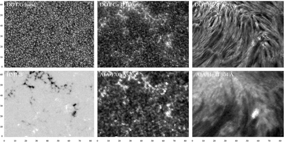
Figure 1: Co-spatial simultaneous images from the Dutch Open Telescope (DOT) at %RE␣I␣found␣that␣setting␣captions␣in␣footnotesize␣comes␣closest%RE␣in␣mimicking␣the␣actual␣A&A␣production␣format.␣␣It␣should␣be␣part%RE␣of␣the␣aa.cls␣style␣file.ftp://dotdb.strw.leidenuniv.nl and from the Solar Dynamics Observatory (SDO) at %****␣aa18525.tex␣Line␣175␣****http://lmsal.com/get_aia_data. First row: DOT images sampling the G band, the core of Ca ii  H with 1.4 Å passband, the center of H $\alpha$ with 0.25 Å passband. Second row: SDO/HMI magnetogram, SDO/AIA 1700 Å image, SDO/AIA He II 304 Å image. They were all taken on September 27, 2010 within a few seconds around 13:54:30 UT, a moment of excellent seeing at the DOT (Fried parameter $r_{0}\!\approx\!14$ cm). The field of view (scales in arcsec, terrestrial North up) is near disk center, South of the largest sunspot of AR11109. It contains a ridge of plage in its upper half, quieter areas in its lower half. The greyscales have been optimized by clipping (all images) and logarithmic scaling (AIA images). We invite the reader to zoom in with a pdf viewer for better appreciation of the detail in the DOT images. DOT observer: E. Romashets. DOT speckle reconstruction: A. Sukhorukov. Alignment routines: P. Sütterlin.

2 Observation

In this section we briefly review the observational character of the chromosphere, as counterpart to the standard-model definition as the domain between the model’s temperature minimum and steep temperature rise towards the corona. Figure 1 gives an overview of the appearance of the solar atmosphere in an area containing plage and network. We use it to demonstrate that the actual chromosphere may have enough opacity to supply significant backradiation in H $\alpha$, but not in the 1700 Å continuum.

The G-band image and the magnetogram in the first column of Fig. 1 are photospheric. The first image displays the granulation and the spatial distribution of small kilogauss magnetic concentrations qualitatively and without sign through their proxy as intergranular bright points (best seen when zooming in). The second image quantifies the actual surface distribution of the line-of-sight component in such strong-field concentrations, but at lower angular resolution. The correspondence is excellent.

The other four images allegedly sample the chromosphere (1700 Å, Ca ii  H, H $\alpha$) and the transition region (He II 304 Å). However, only the H $\alpha$ image truly shows the chromosphere. It consists of long slender fibrils that cover and obscure the photosphere everywhere in the form of overlying fibrilar canopies. This is always the case near active regions, plage, and active network; only the very quietest internetwork areas are not covered by fibrils in H $\alpha$ (e.g., Plate 3.1 of Bray & Loughhead 1974; Rouppe van der Voort et al. 2007; Rutten et al. 2008). These ubiquitous H $\alpha$ fibril canopies constitute the ring of pink emission just off the limb around the Sun that Lockyer (1868) named “chromosphere”. They are also likely to irradiate the low-opacity domain underneath with H $\alpha$ backradiation. Their geometry remains unknown; the fibrilar appearance in images as this one may represent long slender cylindrical fluxtubes (e.g., Heinzel & Schmieder 1994), density variations that cause corrugations of the $\tau\!=\!1$ Eddington-Barbier surface in an extended atmosphere (Schoolman 1972), or warps in sheets as proposed by Judge et al. (2011).

The 1700 Å continuum shows no fibril canopies covering internetwork areas but the underlying domain of cool gas that is every few minutes ridden through by successive hot shocks producing Ca ii H_2V and K_2V cell grains (Rutten & Uitenbroek 1991; Carlsson & Stein 1997; cf. Rutten 2011). It is called “clapotisphere” here following Rutten (1995) and is badly represented by the hydrostatic standard models (Carlsson & Stein 1995). The bright points marking magnetic concentrations and making up the network and plage are roughly co-spatial with the deeper G-band bright points. Their large brightness contrast represents a mixture of scattered hot-wall radiation from below and current heating (Carlsson et al. 2010). Numerical simulations suggest that, due to the latter heating, magnetic concentrations do contain temperature stratifications resembling the standard models (e.g., the FAL-C model of Fontenla et al. 1993), but with the temperature minimum shifted down to height $h\!\approx\!150$ km, still within the photosphere, due to fluxtube evacuation (first quartet in Fig. 9 of Leenaarts et al. 2010). Ubiquitous shocks occur also in and near these concentrations, but also already deeper than in the shocked internetwork clapotisphere (Steiner et al. 1998; Rutten et al. 2011). Slow hydrogen ionization/recombination balancing in the cool aftermath of the shocks causes large NLTE overpopulation of the lower level of H $\alpha$ (Leenaarts et al. 2007).

The Ca ii  H image is much like the 1700 Å image, apart from difference in angular resolution. In the internetwork it shows a bright mesh pattern that is dominated by shock interference and changes rapidly. There are no chromospheric fibrils. One should rather expect that fibrils that are opaque in H $\alpha$ are also opaque at the center of Ca ii  H, because the thicker parts of H $\alpha$ fibrils are seen also in Ca II 8542 Å (Cauzzi et al. 2009), and Ca ii  H is bound to exceed Ca II 8542 Å in extinction. Indeed, in the VAL3-C model Ca ii K₃ forms higher than the core of H $\alpha$ (Fig. 1 of Vernazza et al. 1981). However, filtergrams such as this one are made with wide passbands (1.4 Å for the DOT) so that the internetwork scene is dominated by shock brightness in the inner line wings that swamps the signature of very dark fibrils at line center (Reardon et al. 2009). Compared to the 1700 Å image, there is an extra contribution in the form of a diffuse bright haze around network and plage that is likely the unresolved appearance of the highly dynamic features seen as Ca ii  H straws near the limb (Rutten 2006), Ca ii  H spicules-II outside the limb (De Pontieu et al. 2007b), and RBEs (rapid blue excursions) on the disk in the blue wing of H $\alpha$ (Rouppe van der Voort et al. 2009).

The He II 304 Å image shows fibrilar patterns that are not identical to but also not unlike the H $\alpha$ canopies. It also shows similar bright grains near fibril feet as H $\alpha$ does. These are not cospatial with the bright grains in the G-band and Ca ii  H images. The overall similarity suggests that hot transition-region gas shares the field-guided topography of the H $\alpha$ chromosphere, outlining similar magnetic connectivity patterns. Such patterns seem also to be mapped by Ly$\hskip 0.86108pt\alpha$ fibrils in VAULT images (Vourlidas et al. 2010). Any fibril that is opaque in H $\alpha$ must be very thick in Ly$\hskip 0.86108pt\alpha$ but, comparably to Ca ii  H, the cell-covering fibrils are very dark in Ly$\hskip 0.86108pt\alpha$  whereas other structures, likely Doppler-shifted out of line-center obscuration, contribute larger brightness in the profile-summed VAULT images (Koza et al. 2009).

The conclusion from this section is that significant chromospheric backradiation may be expected in H $\alpha$ and in He II 304 Å which show opaque fibrilar canopies that constitute the actual chromosphere. Ca ii  H should show them too at line center, but the DOT image and all other H & K filtergrams have too wide a bandpass. In the 1700 Å image the absence of any fibrilar signature, bright or dark or as erasure of the internetwork pattern seen in Ca ii  H, implies that they are transparent at this wavelength, even for such a not-so-quiet area. Since the backradiation by an optically thin fibril scales with the fibril opacity, it is unlikely that deeper layers are affected by chromospheric backradiation in such ultraviolet continua.

3 Formulation

Fontenla et al. (2009) based their claim of important chromospheric backradiation on their Fig. 4 containing graphs of population departure coefficients $b$ for selected levels of Si i, Si ii, Mg i, MgII, Fe i, and Fe ii. Population departure coefficients measure the ratio of the actual population density (particles cm${}^{-3})$ to the population computed assuming LTE. There are two formats differing in normalization. The first, called “Menzel” here, follows the original use by Menzel & Cillié (1937) who normalized hydrogen populations to the free proton density. The generalization is to use a partial Saha-Boltzmann evaluation to obtain normalization to the next ion stage (Eq. (6.3) of Jefferies 1968; Eqs. (13)–(15) of Vernazza et al. 1981). The other format, called “Zwaan” here, follows Wijbenga & Zwaan (1972) and uses the elemental abundance as normalization. The two conventions are (Rutten 2003):

$$b_{i}^{\rm Zwaan}\equiv n_{i}/n_{i}^{\rm LTE}\mbox{\rm\leavevmode\nobreak\ \leavevmode\nobreak\ \leavevmode\nobreak\ \leavevmode\nobreak\ and \leavevmode\nobreak\ \leavevmode\nobreak\ \leavevmode\nobreak\ \leavevmode\nobreak\ }b_{i}^{\rm Menzel}\equiv\frac{n_{i}/n_{i}^{\rm LTE}}{n_{C}/n_{C}^{\rm LTE}},$$ (1)

where $n_{i}$ is the population of level $i$, $n_{C}$ is the total population of the next ion, and the superscript LTE implies a complete solution of the Boltzmann-Saha LTE partitioning equations for the given level and all stages of the element. Sometimes the ion ground state $n_{c}$ is used instead of $n_{C}$ assuming $n_{c}\approx n_{C}$. When the atom or ion containing level $i$ is predominantly ionized, so that $n_{C}\approx n_{C}^{\rm LTE}$ because most particles of the species are in the next-ion stage, then

$$b_{i}^{\rm Menzel}\approx n_{i}/n_{i}^{\rm LTE}\approx b_{i}^{\rm Zwaan},$$ (2)

but when most of the element sits in level $i$ itself then

$$b_{i}^{\rm Menzel}\approx n_{C}^{\rm LTE}/n_{C}\approx 1/b_{C}^{\rm Zwaan}.$$ (3)

The continuum has $b_{C}^{\rm Menzel}\equiv 1$ and the ratio $b_{i}/b_{C}\approx b_{i}/b_{c}$ is the same in both definitions.

Equations (2) and (3) were given as Eqs. (17) and (18) by Vernazza et al. (1981), who used the Menzel definition. Fontenla et al. (2009) did so too (private communication from J. Fontenla). We show results for both definitions here because the Zwaan version gives a more intuitive display of actual population departures for majority stages. For example, the Menzel-coefficient dips for $n=1$ of H i and C i at the temperature minimum in Figs. 30 and 33 of Vernazza et al. (1981) and Figs. 13 and 14 of Fontenla et al. (2007) do not imply that the populations of these levels are out of LTE.

Figure 2: Temperature stratification in some standard models. Solid: FAL-C of Fontenla et al. (1993). Dot-dashed: its AL-C7 update by Avrett & Loeser (2008). Dashed: FCHHT-B of Fontenla et al. (2009). Dotted: radiative-equilibrium model from Kurucz (1979, 1992a, 1992b), extended to larger height assuming constant temperature.

4 Demonstration

We select magnesium for plotting departure coefficients as in Fig. 4 of Fontenla et al. (2009). Magnesium is an important electron donor in the upper photosphere where Mg i has larger Rydberg populations than any other element (Fig. 15 of Carlsson et al. 1992). It has important bound-free edges, at 1621.5 Å (vacuum) from the ground state ($3s^{2}\;{}^{1}\mbox{S}^{e}$) and especially at 2512.4 Å (air) from the first excited level ($3s3p\;^{3}\mbox{P}$). Mg i and Mg ii spectrum formation are characteristic for other abundant metals with low ionization energy (silicon, iron, aluminum). Together, these supply the electrons for the photospheric H${}^{{}^{{}_{-}}}\!$ opacity in the visible and infrared and they dominate the solar continuous opacity from the near-ultraviolet to Ly$\hskip 0.86108pt\alpha$ (Fig. 36 of Vernazza et al. 1981).

Figure 2 displays a selection of standard models. FAL-C of Fontenla et al. (1993) was an update of VAL3-C of Vernazza et al. (1981) with a less steep upper photosphere from the inclusion of the ultraviolet line haze and a different transition region from the inclusion of ambipolar diffusion. A more recent update is the AL-C7 model of Avrett & Loeser (2008), constructed in particular to reproduce the ultraviolet spectrum atlases of Brekke (1993) and Curdt et al. (2001). These spectra are also reproduced by model FCHHT-B of Fontenla et al. (2009), which has a higher-located temperature minimum to accommodate dark infrared CO lines.

The dotted curve in Fig. 2 is a radiative-equilibrium model from Kurucz (1979, 1992a, 1992b), that we extended in Cauzzi et al. (2009) to larger height assuming constant temperature. It is very similar to the FCHHT-B model up to $h\ \!=\!800$ km, but has no chromosphere or transition region and so serves as comparison for the case of no backradiation whatsoever.

We have used the 1D version of the RH code (e.g., Uitenbroek 2001) in a setup with similar content as the PANDORA setup of Avrett & Loeser (2008), although the solving method differs much. RH uses a multi-level accelerated lambda iteration method following Rybicki & Hummer (1991, 1992) – hence the code’s name. We used the 66-level model atom for Mg i of Carlsson et al. (1992) and a 12-level model atom for Mg ii from Uitenbroek (1997). Mg iii is represented by its ground state only. Other elements of which the more important transitions are explicitly evaluated in NLTE are H, Si, Al, and Fe. Partial redistribution is accounted for in Mg ii h & k and Ly$\hskip 0.86108pt\alpha$ and $\beta$. The violet and ultraviolet line haze (e.g., Greve & Zwaan 1980) causing a quasi-continuum is accounted for by sampling the 236 000 lines between $\lambda\!=\!1000$ and 4000 Å in the extensive list of Kurucz every 20 mÅ, using a two-level coherent scattering approximation per wavelength in which the collisional transition probability of each sampled line is estimated from the radiative one with the approximation of van Regemorter (1962), rather than applying a common scattering recipe for all lines as done by Avrett & Loeser (2008). However, a test with the much simpler line-haze recipe of Bruls et al. (1992) showed only little differences with the results shown here.

Figure 3: Upper panels: magnesium ionization fractions $N_{\rm stage}/N_{\rm total}$ in the Kurucz model (left) and the FCHHT-B model (right), with $N_{\rm stage}$ the summed populations per ionization stage, $N_{\rm total}$ the total of all stages. Solid: NLTE. Dashed: LTE. Lower panels: gradient comparisons. The $y$-axis units specify the logarithmic electron density $N_{\rm e}$ and total hydrogen density $N_{\rm H}$ in particles m^-3. The temperature curves show $20\,\log(T)-57$ to provide comparable gradients.

Figure 3 shows the resulting NLTE and LTE ionization fractions for the Kurucz and FCHHT-B models. In both magnesium is virtually once-ionized throughout the atmosphere (below the transition region at $h\!=\!1900$ km for FCHHT-B). Let us first interpret the simple LTE curves in the upper Kurucz panel, which reflect the competing effects in the Saha equation of the outward decreases of the temperature $T$ and electron density $N_{\rm e}$ shown in the lower Kurucz panel. Both decreases are steepest in the deepest layers, where $N_{\rm e}$ drops from $10^{-1}$ to $10^{-4}$ of the hydrogen density $N_{\rm H}$ because hydrogen becomes neutral. The $N_{\rm e}/N_{\rm H}\!\approx\!10^{-4}$ limit represents the combined abundance of the electron donor elements (Fe, Mg, Si, Al) and controls the H${}^{{}^{{}_{-}}}\!$ opacity. The steep $T$ drop wins from the steep $N_{\rm e}$ drop so that the Mg i fraction increases and the Mg iii fraction decreases with height. Around $h\!=\!500$ km the $N_{\rm e}$ drop wins from the $T$ drop so that the LTE Mg i fraction drops slightly. The outer exponential decay of this fraction follows the decreasing gas density (with constant $N_{\rm e}/N_{\rm H}\!\approx\!10^{-4}$) at constant temperature. The NLTE Mg i curve also shows near-exponential decay around $h\!=\!500$ km, implying that the nonthermal contribution, from radiative instead of collisional ionization and recombination, is about constant with height.

The Mg i and Mg iii curves in the FCHHT-B panel are closely the same as in the Kurucz panel up to the FCHHT-B temperature minimum at $h\!=\!800$ km, just as the models are. Thus, up to this height magnesium ionization does not depend much on higher layers.

Figure 4: Population departures of magnesium ground states for the Kurucz model (upper panels) and the FCHHT-B model (lower panels). Left: Zwaan definition. Right: Menzel definition. Solid: Mg i ground state. Dashed: Mg ii ground state. Dot-dashed: Mg iii ground state.

Figure 4 shows the population departures $b$ of the magnesium ground states for the Kurucz and FCHHT-B models. Both $b$ definitions are used (left and right columns). Mg iii cannot be shown in the Menzel version because we do not include Mg iv. Since most of the population per ionization stage resides in the ground state, these curves reflect the divergences between the LTE and NLTE ionization fractions in Fig. 3.

The FCHHT-B/Menzel curves in the last panel resemble the corresponding curves in Fig. 4 of Fontenla et al. (2009), which for Si ii and Fe ii dip yet deeper than for Mg ii. At first sight the two deep dips in this panel would suggest large depletion of both Mg i and Mg ii at the temperature minimum. However, for Mg ii this dip is the reverse of the Mg iii peak in the Zwaan panel following Eq. (3). In the Zwaan panels the Mg ii curves remain near unity because even large overionization of Mg i and overpopulation of Mg iii do not much affect the Mg ii population, being dominant anyhow (Fig. 3).

Near and above the temperature minimum, the Mg i and Mg iii curves in the first panel of Fig. 4 mimic the temperature structure of the model atmosphere, for Mg iii reversely. This implies that the actual degree of ionization does not sense the temperature but is constant with height, so that the departure behavior is set by the LTE Saha-Boltzmann temperature sensitivity. A constant degree of ionization suggests dominance of constant radiation in an optically thin environment.

Figure 5: The Planck function $B_{\nu}$ (solid), mean radiation $J_{\nu}$ (dotted), and source function $S_{\nu}$ (dashed) averaged over the first 100 Å of the Mg i edges with thresholds at $\lambda\!=\!2512.4$ and 1621.5 Å. Left: Kurucz model. Right: FCHHT-B model. Formal representative temperatures are plotted for these quantities: the electron temperature for $B_{\nu}$, radiation temperature for $J_{\nu}$, and excitation temperature for $S_{\nu}$. They are obtained by applying the inverse Planck function to $B_{\nu},J_{\nu},S_{\nu}$, respectively. The dot-dashed distributions at the bottom are the intensity contribution functions $j_{\nu}\,\exp(-\tau_{\nu})$, with $j_{\nu}$ the emissivity and $\tau_{\nu}$ the optical depth,near the thresholds wavelengths. The lefthand deeper-formed curve is for the 2512 Å edge. Each curve is scaled to its maximum value.

5 Explanation

The behavior of $b_{1}^{\rm Zwaan}$ for Mg i in Fig. 4 is well-understood, in particular since the classic PhD analysis of the comparable iron spectrum by Lites (1972) (cf. Athay & Lites 1972; review by Rutten 1988). The deep dip results from the dominance of the radiation field $\overline{J}$ in the source function $\overline{S}$ of the Mg i ionization edges in the violet and ultraviolet, where the bar denotes opacity-weighted frequency averaging over the edge and $J$ is the angle-averaged intensity over all directions.

Figure 5 illustrates this cause by plotting 100 Å-wide averages of $S_{\nu}$, $B_{\nu}$ and $J_{\nu}$ for the two major Mg i edges against height in the Kurucz and FCHHT-B models. The spectral averaging smooths the many superimposed line blends. These quantities are plotted as formal temperatures in order to combine them in single diagrams for the two wavelengths, removing the Planck function sensitivity to wavelength (which is exponential in the Wien approximation valid here). Figure 5 shows that across the ultraviolet $S_{\nu}$ tends to follow $J_{\nu}$ at the heights where the radiation escapes (shown by the contribution functions at the bottom of the graphs), with $J_{\nu}\!\approx\!B_{\nu}$ for the 2512 Å edge.

Single-transition scattering with $\overline{S}\!=\!(1-\varepsilon)\,\overline{J}+\varepsilon\,\overline{B}$ is an excellent approximation for these edges which scatter strongly, with complete redistribution over the edge profile. The steep decrease of the collisional destruction probability $\varepsilon$ with height makes $\overline{S}$ uncouple from $\overline{B}$ already deep in the photosphere, at a thermalization depth much deeper than the radiation escape depth. The sensitivity of the $\bf\Lambda$ operator to the steepness of the $S_{\nu}(\tau)$ gradient results in $J_{\nu}>B_{\nu}$ where they uncouple. This excess produces a superthermal edge source function in the upper photosphere, with $\overline{S}\approx(b_{c}/b_{i})\,\overline{B}$ in the Wien limit for an edge between level $i$ and ionization limit $c$. Thus, the divergence between $S_{\nu}$ and $B_{\nu}$ for the edge at 1621.5 Å in Fig. 5 translates into the divergences between $b_{c}$ (Mg ii) and $b_{1}$ (Mg i) in Fig. 4 that measure the source function departure from LTE for this edge. Similarly for $b_{c}/b_{2}$ in the edge at 2512.4 Å (which is a more important ionization channel and continuum provider).

In a plane-parallel atmosphere $J_{\nu}$ flattens out to a constant outer limit unless there is significant emissivity in higher layers. The 1D models have that in their transition regions where the steeply increasing temperature gives larger $\varepsilon$, causing renewed coupling to $B_{\nu}$. Below the transition region, the flat $J_{\nu}$ may cut through whatever the model specifies as chromospheric temperatures, so that the latter are mapped into the $b_{c}/b_{i}$ ratio when $S_{\nu}$ follows $J_{\nu}$. In the FCHHT-B panel of Fig. 5 the 2512.4 Å edge shows such behavior. The 1621.5 Å edge has some $S_{\nu}$ coupling to the higher chromospheric temperature and a yet smaller increase in $J_{\nu}$, which rises slightly above the flattened-out limit value for the Kurucz model.

All this is beautifully illustrated across the VAL3-C spectrum in Fig. 36 of Vernazza et al. (1981) and is explained at length in Rutten (2003).

There is no significant difference between the two models in Fig, 5 at the heights of formation of these bound-free Mg i continuum contributions. For both edges the formation is purely photospheric. Backradiation from the upper chromosphere plays no role.

The conclusion from Figs. 2–5 is that the FCHHT-B model differs quantitatively from VAL3-C, but not qualitatively and not in its radiation physics. In particular, the continuum formation at these ultraviolet wavelengths is identical between the two models used here since the differences in $S_{\nu}$ at larger heights are not sampled by the photospheric contribution functions.

Figure 6: Population departures of selected magnesium levels in the FCHHT-B model. The level numbers increase with excitation energy. Left: Mg i. Right: Mg ii. Upper row: Zwaan definition. Lower row: Menzel definition.

Figure 6 adds FCHHT-B $b$ curves for selected excited levels in Mg i and Mg ii to the ground-state display in the upper panels of Fig. 4. The Mg i ground state has the largest NLTE deficit in the temperature minimum due to $\overline{J}>\overline{B}$ overionization in the principal Mg i edges. The plateau of $b_{1}$ (index 0) excess at larger height maps $\overline{J}<\overline{B}$ in these scattering edges.

The higher levels in Mg i converge to the $b\!\approx\!1$ value of the Mg ii ground state, with multi-level crosstalk (“interlocking”). In the Mg i Rydberg domain this convergence is maintained by a collisional population replenishment flow driven by photon losses in intermediate Mg i lines, exemplified by the deep onset of the drop in the $n\!=\!10$ curve. Such photon-loss replenishment from the next-ion population reservoir was called photon suction by Bruls et al. (1992). The Rydberg flow causes the Mg i emission features near $\lambda\!=\!12$ $\mu$m that were thought chromospheric by Zirin & Popp (1989), but actually are photospheric (Carlsson et al. 1992).

The Mg ii $b$ peaks in the second panel of Fig. 6 reflect the effect of $\overline{J}>\overline{B}$ pumping in strong ultraviolet lines, similarly as in Fe ii (see Rutten 1988). A particular example of the latter is the weak Fe ii 3969.4 Å line between Ca ii  H and H $\epsilon$, discovered as limb emission line by Evershed (1929). Its on-disk emission was initially attributed to chromospheric backradiation by Lites (1974), but is actually caused by photospheric pumping in Fe ii resonance lines (Cram et al. 1980) which explains its extraordinary spatial intensity variation at the limb (Rutten & Stencel 1980). Similar upper-photosphere $\overline{J}>\overline{B}$ pumping sets the $b$ peak of the Mg iii ground state in the first panel of Fig. 4.

The lower panels of Figure 6 repeat the $b$ displays for the Menzel definition. The lefthand panels are the same, but on the right the Menzel panel shows reversals of the Zwaan panel due to the normalization by the Mg iii population. It makes the Mg ii curves appear similar to the Mg i curves.

The lower panels of Figure 6 are similar to the corresponding Mg i and Mg ii panels in Fig. 4 of Fontenla et al. (2009). The look-alike sequences of dips, deepest for the lowest levels, in their six Menzel plots made Fontenla et al. (2009) conclude: “All our results display overionization (i.e., ground-level departure from LTE coefficients smaller than unity) of all species around the temperature minimum. […] Also, near the temperature minimum the lower levels have smaller departure coefficients than the upper levels, indicating that the overionization of neutrals is a result from FUV and/or EUV irradiation which primarily affects lower levels. This indicates that overionization is much more affected by the irradiation from the upper chromosphere in continuum and emission lines than by the photospheric radiation and absorption lines. Therefore, we stress that the consideration of a realistic upper chromosphere is essential to the determination of the densities near the temperature minimum of (1) neutral low first-ionization-potential (FIP) elements, and (2) singly ionized high FIP elements. Even a very sophisticated calculation of the effects of lower chromospheric absorption lines on the elemental ionization can produce unrealistic results if it does not include upper chromosphere irradiation.”. This interpretation is incorrect. Downward irradiation does not affect the degree of ionization of these minority species around the temperature minimum of the FCHHT-B model. We have demonstrated this for Mg here; the same applies to Fe, Si, Al.

However, more positively, we wish to note that the modeling of Fontenla et al. (2009) is not impaired by this misinterpretation of its results, and that that does not detract value from their effort. In this era of giant computer programs it becomes non-trivial to diagnose what the output implies. Chromospheric physics is becoming a key area in solar research but does require understanding of complex non-equilibrium optically-thick spectrum formation. Our tutorial elucidation of this particular issue may be instructive to newcomers to the field.

Figure 7: H $\alpha$ formation for the Kurucz (left) and FCHHT-B (right) models. Solid: Planck function $B_{\nu}$ at line center. Dashed: angle-averaged radiation $J_{\nu}$ at line center. Dotted: total source function $S_{\nu}$ at line center. The ticks mark the locations with line-center optical depth $\tau_{\nu}=3,1,0.3$ from left to right.

6 Backradiation in H$\alpha$

Figure 7 shows formation parameters for H $\alpha$ in the Kurucz and FCHHT-B models. It is similar to Fig. 8 in Cauzzi et al. (2009), but here, prompted by the referee and in the vein of this paper, we add detailed analysis using the FCHHT-B model for demonstration. We do not regard it a viable explanation of actual solar H $\alpha$ formation (Sect. 7), but use it rather as a one-dimensional didactic “FCHHT-B star”.

The lefthand panel of Fig. 7 illustrates H $\alpha$ line formation in such a star without overlying chromosphere. At line center, $J_{\nu}$ drops well below $B_{\nu}$. This behavior differs from the $J_{\nu}\!>\!B_{\nu}$ excesses of the ultraviolet continua in Fig. 5 because the Planck-function sensitivity to temperature is smaller at longer wavelengths, flattening the ${\rm d}B_{\nu}/{\rm d}h$ gradient, and because the substantial additional line opacity $\alpha^{l}_{\nu}$ flattens the ${\rm d}B_{\nu}/{\rm d}\tau_{\nu}={\rm d}B_{\nu}/[(\alpha_{\nu}^{c}+\alpha_{\nu}^{l})\,{\rm d}z]$ gradient yet more. The $\bf\Lambda$ operator then produces $J_{\nu}<S_{\nu}$ tending towards the $S_{\nu}(0)=\sqrt{\varepsilon_{\nu}}B_{\nu}$ surface value for a scattering isothermal atmosphere with constant $\varepsilon_{\nu}$.

In the Kurucz model the H $\alpha$ core originates from the upper photosphere around $h\!=\!400$ km as a deep, strongly scattering line with $S_{\nu}\approx\overline{J}_{\nu_{0}}$. The corresponding emergent profile is shown in the top panel of Fig. 8. It is well reproduced by applying the Eddington-Barbier approximation $I_{\nu}\approx S_{\nu}(\tau_{\nu}\!=\!1)$.

Figure 8: Top panel: emergent H $\alpha$ intensity profiles at disk center computed from the FCHHT-B (dotted) and Kurucz (dashed) models, in comparison with the observed spatially-averaged profile (solid) taken from the atlas observed by Brault & Testerman, calibrated by Neckel & Labs (1984), and posted by Neckel (1999). Lower panels: mean intensity $J_{\nu}$ across H $\alpha$ at different heights in the Kurucz and FCHHT-B atmospheres, respectively. For the Kurucz panel the sampling heights are 26, 41, 157, 283, 358 and 995 km. For the FCHHT-B panel they are 35, 150, 300, 519, 850, 1000, 1340 and 1701 km. The dotted profile in the bottom panel is the outward intensity at height 850 km, impinging on the FCHHT-B chromosphere. The dotted profile in the middle panel is the outward intensity at height 252 km in the Kurucz model where the line-center optical depth equals the optical thickness $\tau_{\nu}=3.5$ of the FCHHT-B chromosphere.

Figure 9: Solid: H $\alpha$ line extinction coefficients $\alpha_{\nu}^{l}$ per m against height for the FCHHT-B model, at line center and in the blue wing at $\Delta\lambda\!=\!-0.44$ and $-0.74$ Å, and the continuous opacity $\alpha_{\nu}^{c}$ in the adjacent continuum. The dot-dashed curve is the line-center result for LTE. The opacities are multiplied by a scale height of $10^{5}$ m to make them comparable to the corresponding optical depth scales (dotted curves). The tick marks on the latter correspond to $\tau_{\nu}=3,1,0.3$. Across the opacity dip due to the temperature minimum the optical depth is $\tau_{\nu}=3.5,0.7,0.04$ at the three line wavelengths, respectively.

The righthand panel of Fig. 7 shows the formation of H $\alpha$ in the FCHHT-B model. Its chromospheric high-temperature plateau supplies sufficient H $\alpha$ opacity that at line center $\tau_{\nu}\!=\!1$ is reached about a thousand km higher than in the Kurucz model. The line-center formation is again well described by $I_{\nu}\approx S_{\nu}(\tau_{\nu}\!=\!1)\approx\overline{J_{\nu_{0}}}(\tau_{\nu}\!=\!1)$, but the Eddington-Barbier approximation is less well applicable in the line wings which have a formation gap between photosphere and chromosphere (e.g., Schoolman 1972; Leenaarts et al. 2006). This gap is detailed in Fig. 9 which shows H $\alpha$ opacities and optical depth scales, with the opacities multiplied by the scale height in the upper FCHHT-B photosphere (it doubles in the FCHHT-B chromosphere from a steep increase of the imposed non-gravitational acceleration). The line extinction has a deep dip in the temperature minimum. Correspondingly, the optical depth buildup (dotted curves) levels out. At line center the FCHHT-B chromosphere has optical thickness $\tau_{\nu}\!=\!3.5$. At $\Delta\lambda\!=\!-0.44$ Å $\tau_{\nu}\!=\!0.3$ (outer tick) is reached already in the chromosphere but $\tau_{\nu}\!=\!1$ only a thousand km deeper in the photosphere. At $\Delta\lambda=-0.74$ Å the FCHHT-B chromosphere is virtually transparent.

At line center the line extinction much exceeds the continuous extinction even in the dip, so that the total source function equals the line source function at all heights. In the wings the line extinction drops below the continuum extinction. Where this happens the total source function drops to the Planck function (not shown).

Figure 10: H $\alpha$ population departure coefficients against height for the FCHHT-B model. The tick marks correspond to $\tau_{\nu}=3,1,0.3$. Solid: lower-level departure coefficient $b_{2}$. Dashed: upper-level departure coefficient $b_{3}$.

Figure 10 shows the departure coefficients $b_{2}$ and $b_{3}$ (Zwaan definition) governing H $\alpha$ in the FCHHT-B model. The curve divergence $\log(b_{3})-\log(b_{2})$ corresponds to the curve divergence $\log(S_{\nu})-\log(B_{\nu})$ in the FCHHT-B panel of Fig. 7. Throughout the near-isothermal FCHHT-B chromosphere the H $\alpha$ opacity is nearly in LTE because the formation of Ly$\hskip 0.86108pt\alpha$ is close to detailed balancing there. However, this is not the case in the deep temperature minimum and steep rise to the chromospheric temperature. Here the $\bf\Lambda$ operator smooths the rapid temperature changes for the scattering-dominated Ly$\hskip 0.86108pt\alpha$ source function (not shown) which has $\overline{S_{\nu}}\approx\overline{J_{\nu}}\approx b_{2}\,B_{\nu}$. This Ly$\hskip 0.86108pt\alpha$ smoothing causes the high peak in $b_{2}$ and considerable corresponding fill-in of the opacity dips in Fig. 9, illustrated for line center as difference with the much deeper dot-dashed LTE curve. In this manner Ly$\hskip 0.86108pt\alpha$ scattering compensates for low-temperature H $\alpha$ opacity loss when cool features are narrow in spatial extent. The $b_{2}$ peak in Fig. 10 doubles if CRD is adopted for Ly$\hskip 0.86108pt\alpha$, from additional smoothing through farther wing-photon travel.

The corresponding emergent intensity profile in the top panel of Fig. 8 is similar to the Kurucz result despite the disparate line formation. Both are reasonably good approximations to the observed mean quiet-Sun profile. Both gain fit quality in the wings if the computed continuum intensity is rescaled to the observed value. Increase of the microturbulence in the Kurucz model from 1.5 to about 10 km s^-1 produces a good core fit for this model as well.

The $J_{\nu}$ curves in Fig. 7 show that the opacity gap in the FCHHT-B model contains much more H $\alpha$ radiation than at corresponding heights in the Kurucz model. This H $\alpha$ radiation fill-in causes a yet higher peak for $b_{3}$ in Fig. 10. It is detailed in the lower panels of Fig. 8. In the lower photosphere the H $\alpha$ $J_{\nu}$ profiles are the same for the two models, but above $h\approx 250$ km the Kurucz model gives absorption cores whereas the FCHHT-B model predicts slightly self-reversed cores across the opacity gap. This difference explains that for the Kurucz model $\overline{J}_{\nu_{0}}$ (shown by the line-center $S_{\nu}$ curve in the lefthand panel of Fig. 7) ends up higher than $J_{\nu}$ at line center, whereas for the FCHHT-B model $S_{\nu}\approx\overline{J}_{\nu_{0}}$ coincides with line-center $J_{\nu}$ across the opacity gap in the righthand panel of Fig. 7. The large core width of the highest-formed FCHHT-B profiles comes from large thermal broadening (about 10 km s^-1) and yet larger microturbulence (about 15 km s^-1).

Because the FCHHT-B chromosphere is near-isothermal the H $\alpha$ formation is comparable to the classic results for a finite isothermal scattering atmosphere of Avrett & Hummer (1965), in particular their optically thick but effectively thin case in which the line source function does not reach thermalization. The main difference is that the FCHHT-B chromosphere is irradiated from below. The impinging intensity profile in the outward direction is shown by the dotted curve in the bottom panel of Fig. 8. This line is much shallower than the emergent profile from the Kurucz model, in agreement with the much higher $J_{\nu}$ above $h\!\approx\!200$ km. A test with a hotter chromosphere, i.e., thicker in H $\alpha$, gives more backradiation and a higher impinging profile with a bright self-reversed core. However, the deep emergent-intensity core remains about the same.

Thus, the presence of an opaque chromosphere changes the illumination profile with respect to the profile that emerges from the same photosphere without overlying chromosphere. A mathematical explanation is given by the principle of invariance (page 165 of Chandrasekhar 1950) regarding addition or subtraction of a layer of arbitrary optical thickness to a semi-infinite plane-parallel atmosphere; creating a gap or pushing down the finite chromospheric atmosphere over the gap to where it meets similar source conditions does not change the emergent radiation. A more physical explanation is that the radiation field in the gap builds up due to backradiation from the overlying chromosphere (called reflection by Chandrasekhar 1950).

Figure 11: H $\alpha$ source function comparisons for the FCHHT-B model. Solid: Planck function and total source function at line center. The latter has ticks at $\tau_{\nu_{0}}=3,1,0.3$. Dotted: line source function $S^{l}_{\nu_{0}}$, differing from the total source function only at the very top of the atmosphere. Dashed and dot-dashed: two-level approximation $(1-\varepsilon_{\nu_{0}})\,\overline{J}_{\nu_{0}}+\varepsilon_{\nu_{0}}B_{\nu_{0}}(T)$ and profile-averaged mean intensity $\overline{J}_{\nu_{0}}$. These coincide everywhere.

We now demonstrate that this backradiation is dominated by two-level scattering. The line source function for complete redistribution can be written as:

$$S^{l}_{\nu_{0}} = (1-\varepsilon_{\nu_{0}}-\eta_{\nu_{0}})\,\overline{J}_{\nu_{0}}+\varepsilon_{\nu_{0}}B_{\nu_{0}}(T)+\eta_{\nu_{0}}B_{\nu_{0}}(T_{\rm d})$$ (4)

$$= \frac{\overline{J}_{\nu_{0}}+\varepsilon_{\nu_{0}}^{\prime}B_{\nu_{0}}(T)+\eta_{\nu_{0}}^{\prime}B_{\nu_{0}}(T_{\rm d})}{1+\varepsilon_{\nu_{0}}^{\prime}+\eta_{\nu_{0}}^{\prime}},$$ (5)

where $\overline{J}_{\nu_{0}}$ is the profile-averaged mean intensity, $\varepsilon_{\nu_{0}}$ the thermal destruction probability, i.e., the fraction of line-photon extinctions by direct collisional deexcitation corrected for emissivity from spontaneous scattering, $\eta_{\nu_{0}}$ the fractional probability of all indirect detour extinction, with detour meaning any multi-level path from the upper to the lower level not including the direct transition, corrected for stimulated detour emissivity, and $\varepsilon_{\nu_{0}}^{\prime}$ and $\eta_{\nu_{0}}^{\prime}$ the corresponding ratios of such extinctions to the contribution by two-level scattering. The formal detour excitation temperature $T_{\rm d}$ is given by $(g_{u}\,D_{ul})/(g_{l}\,D_{lu})\equiv\exp(h\nu_{0}/kT_{\rm d})$ where $D_{ul}$ is the summed transition probability (per second per particle in the upper level) of all detour upper-to-lower paths, $D_{lu}$ for all detour lower-to-upper paths, and $g_{l}$ and $g_{u}$ are the statistical weights.

The classic literature used Eq. 5 (e.g., Gebbie & Steinitz 1974; Sect. 8.1 of Jefferies 1968; Eq. 12.11 of Mihalas 1970) following Thomas (1957) who divided strong lines into “collision type” with $\varepsilon_{\nu_{0}}>\eta_{\nu_{0}}$ and “photoelectric type” with $\eta_{\nu_{0}}>\varepsilon_{\nu_{0}}$, designating H $\alpha$ as principal example of the second type. In particular, H $\alpha$ would gain most photons from Balmer ionization followed by a recombination path into $n\!=\!3$ employing photospheric Balmer photons (e.g., Athay & Thomas 1961; see also Cram 1985). The corresponding schematic source function diagram in Fig. 3 of Jefferies & Thomas (1959) (reprinted in Fig. 12-9 of Mihalas 1970 and Fig. 11-11 of Mihalas 1978) is qualitatively similar to the FCHHT-B H $\alpha$ behavior in Fig. 7, with $S_{\nu}^{l}$ leveling out in the photosphere to become much higher than $B_{\nu}$ in the temperature minimum.

Figure 12: Fractional collisional contribution $\varepsilon_{\nu_{0}}[B_{\nu_{0}}(T)\!-\!\overline{J}_{\nu_{0}}]/S^{l}_{\nu_{0}}$ (dashed) and detour contribution $\eta_{\nu_{0}}[B_{\nu_{0}}(T_{\rm d})\!-\!\overline{J}_{\nu_{0}}]/S^{l}_{\nu_{0}}$ (dot-dashed) to the H $\alpha$ line source function. Their sum (solid) represents $(S^{l}_{\nu_{0}}-\overline{J}_{\nu_{0}})/S^{l}_{\nu_{0}}$. The ticks on the $x$-axis are at $\tau_{\nu_{0}}\!=\!3,1,0.3$ in H $\alpha$.

However, in the FCHHT-B case this behavior is due to the backscattering from the chromosphere, not from Balmer-continuum detour emission. If the latter were important it would raise the H $\alpha$ source function also for the Kurucz model. The Balmer continuum scatters outward similarly to the 2512 Å continuum in Fig. 5, the same in both models up to $h\approx 800$ km, with about 1400 K radiation temperature excess in the temperature minimum – but that region is transparent in H $\alpha$.

The scattering nature of the H $\alpha$ source function is demonstrated in Fig. 11 by comparing it with the mean radiation $\overline{J}_{\nu_{0}}$ and the two-level approximation. They are closely the same everywhere. The differences are magnified in Fig. 12 showing the fractional collision and detour contributions. The collisional contribution is negligible except in the deep photosphere where collisional excitations create most H $\alpha$ photons (with $\varepsilon_{\nu_{0}}\!\approx\!1$ and $\overline{J}_{\nu_{0}}\!\approx\!B_{\nu_{0}}$). The latter resonance-scatter outward. Higher up, the detour contribution is much larger, confirming the $\eta_{\nu_{0}}/\varepsilon_{\nu_{0}}$ evaluation of Al et al. (2004), but it still amounts to only a few percent of the line source function and raises the line-center intensity by only one percent of the continuum intensity. In the steep temperature rise of the FCHHT-B transition region the detour contribution grows rapidly to nearly 100%, but at negligible H $\alpha$ opacity and therefore of no importance to the emerging profile – and not due to photospheric irradiation.

The conclusion from this section is that in the FCHHT-B model H $\alpha$ is first and foremost a scattering line, with chromospheric backscattering boosting the line-center radiation across the opacity gap between photosphere and chromosphere. The H $\alpha$ core emerges from the FCHHT-B chromosphere but most photons were created in the deep photosphere. For H $\alpha$ the FCHHT-B chromosphere is primarily a scattering attenuator that builds up its own irradiation from below. The main source function difference with other strong scattering lines such as the Ca ii resonance lines and infrared triplet is the effect of the opacity gap, not the amount of detour contribution.

7 Discussion

Static 1D modeling of the continua from the solar atmosphere has reached such sophistication that even the modelers themselves may misinterpret their results (Sect. 5). Interpretation of chromospheric fine structure using strong lines, in particular H $\alpha$, has relied more on cloud modeling (see the excellent review by Tziotziou 2007) than on static model-atmosphere interpretation as in Sect. 6. In the meantime, observations of the actual chromosphere (Sect. 2) have reached such spatial and temporal resolution that the worlds of the modelers and the observers now seem far apart. A third worldview is given by time-dependent numerical MHD simulations of the chromosphere (e.g., Schaffenberger et al. 2006; Leenaarts et al. 2007, 2010; Martínez-Sykora et al. 2011). Obviously, the different views should come together. It falls outside the scope of this paper to effectuate such synthesis, but we make a few salient points.

Emergent spectrum fitting.

The FCHHT-B model and the AL-C7 model of Avrett & Loeser (2008) fit the ultraviolet atlases about equally well, but differ appreciably in their stratifications (Fig. 2) and in their stratification physics. Both assume hydrostatic equilibrium, but the AL-C7 model gains additional chromospheric support from imposed turbulent pressure inspired by observed line broadening, as in its VAL and FAL predecessors. The FCHHT-B model gains chromospheric support instead from imposed non-gravitational acceleration inspired by the Farley-Buneman instability (Fontenla et al. 2008). Thus, best-fit model determination from such data does not represent a unique data inversion.

An extreme example of non-uniqueness is that the two disparate H $\alpha$ formations in Fig. 7, with and without a chromosphere, can both fit the observed average H $\alpha$ profile (top panel of Fig. 8). Figure 1 obviously suggests that chromospheric H $\alpha$ formation as in the FCHHT-B model is more realistic than photospheric H $\alpha$ formation as in the Kurucz model, but the predicted H $\alpha$ profile cannot be used as discriminator.

One-dimensional continuum modeling.

The similarity of the magnetogram, 1700 Å and Ca ii  H panels in Fig. 1 suggests that 1D modeling along vertical columns which differs between internetwork, network, and plage may be a reasonable approximation for ultraviolet continua from these features. The bright grains that constitute network and plage mark strong-field structures that are roughly vertical. However, facular modeling towards the limb must then account for slanted viewing across such structures by cutting through different 1D models along the line of sight, as in the classic Zürich fluxtube modeling of e.g., Bünte et al. (1993).

Cloud modeling.

The FCHHT-B chromosphere may be regarded as an horizontally extended isothermal slab but not as a constant-property cloud since it is more like a finite atmosphere, with density stratification, outward $S_{\nu}$ decay, and Eddington-Barbier-like H $\alpha$ core formation. The source function is dominated by scattering (Fig. 11) and the slab is effectively thin (Fig. 9) so that the source function amplitude depends on the slab opacity. Due to backscattering, the H $\alpha$ profile illuminating the slab from below (dotted curve in the bottom panel of Fig. 8) is shallower than for locations without an overlying chromospheric blanket (Kurucz prediction in the top panel of Fig. 8; cf. Bostanci & Al Erdoğan 2010) and brightens for a thicker blanket. If actual fibrilar canopies share such properties than these upset classical cloud modeling.

At the suggestion of the referee, we added in the middle panel of Fig. 8 the outward intensity profile at that optical depth in the Kurucz model which equals the optical thickness of the FCHHT-B chromosphere. It is similar to the outward intensity profile impinging the latter (bottom panel) because the line formation is much more similar for the two models on optical depth scales than on geometrical height scales. The near-equality of these profiles suggests a new recipe for 1D H $\alpha$ cloud modeling, namely to use the outward intensity profile in a radiative-equilibrium photosphere at optical depth equal to the cloud’s thickness as impinging background profile.

Dynamics.

The actual internetwork atmosphere above the photosphere (in our view consisting of a cool clapotisphere, chromospheric fibril canopy, and a similar-morphology sheath-like transition region) is continuously shocked. In H $\alpha$ ubiquitous internetwork shocks are evident in Doppler timeslices (e.g., Rutten et al. 2008; Cauzzi et al. 2009). In magnetic concentrations shocks are ubiquitous already in the photosphere. Shocks also produce the dynamic fibrils jutting out from network (Hansteen et al. 2006; De Pontieu et al. 2007a). The elusive straws / spicules-II / RBEs near network are even more dynamic. This basic chromospheric dynamism upsets static chromosphere modeling.

Departures from LTE.

The FCHHT-B NLTE departures discussed here reach two to three orders of magnitude at the FCHHT-B temperature minimum (Figs. 4, 10) while the lower level of H $\alpha$ is nearly in LTE where the line forms (Fig. 10). The non-equilibrium simulation of Leenaarts et al. (2007) predicts overpopulations of this level up to twelve orders of magnitude for cool post-shock phases, where the temperature may fall well below the temperature minima of the standard models (Leenaarts et al. 2011). Thus, dynamic behavior may dramatically increase the temperature variations and NLTE effects.

Height of the transition region.

One-dimensional models for different features typically differ primarily in the height of their transition region. Simulations as the one of Leenaarts et al. (2007) suggest that the transition region above internetwork is kicked up and mass-loaded by field-guided flows that do not obey one-dimensional hydrostatic equilibrium. In this simulation the location of the transition region varies over $h\!=\!1000-4000$ km, with rapid changes, and is generally lower above magnetic concentrations. Such larger range than in the 1D model grids may better reflect actual variations in fibril-canopy height or corrugation.

H $\alpha$ opacity gap.

The H $\alpha$ opacity gap and backscattering into it are properties of the FCHHT-B model. Do they also occur in the real Sun? The images in Fig. 1 roughly agree with FCHHT-B predictions: in the 1700 Å image no fibrils are seen whereas they appear opaque in the H $\alpha$ image. Also, when one samples the real Sun in H $\alpha$ away from line center (e.g., in DOT movies) the photospheric granulation appears when the fibrils become transparent, without an intermediate clapotispheric scene as in the Ca ii  H and 1700 Å images in Fig. 1. Thus, a similar opacity gap seems to exist under the actual fibrilar canopies making up the internetwork chromosphere. The radiation crossing it, boosted by backscattering, will suffer substantial spatial smoothing of the photospheric scene. Some of it may leak out through an effectively thin fibril canopy, scatter around dark fibrils in photon channeling as suggested by Al et al. (2004), or be seen from aside as in the backradiation explanation of bright rims under filaments (e.g., Kostik & Orlova 1975; cf. Panasenco 2010).

H $\alpha$ detour brightening.

In the FCHHT-B model H $\alpha$ is an almost pure scattering line (Fig. 11). The detour contribution $\eta_{\nu_{0}}(B_{\nu_{0}}(T_{\rm d})-\overline{J}_{\nu_{0}})$ to the line source function becomes important only in the transparent transition region (Fig. 12). In the real Sun locations with very bright H $\alpha$, such as the moss and active-region heart in Fig. 13 of Rutten (2007), may represent low-lying, denser transition regions that radiate H $\alpha$ through recombination paths.

8 Conclusion

The development of standard models of the solar atmosphere, masterminded by E.H. Avrett, represents a well-established pinnacle of sophistication with respect to the application of NLTE spectrum formation theory with the inclusion of numerous spectral features. However, the assumption of hydrostatic and time-independent equilibria without magnetism remains a far cry from the actual solar chromosphere, which is pervaded by shocks and rapidly changing magnetic fine structure in even the quietest regions.

Conversely, state-of-the-art magnetohydrodynamics simulations do a good job in emulating the small-scale magnetodynamism of the actual solar atmosphere, but they remain weak in properly treating non-equilibrium radiation. Implementation of the art of the 1D modelers into the 3D time-dependent codes of the simulators presents a formidable challenge, but seems the most promising venue to understand the enigmatic solar chromosphere (cf. Leenaarts et al. 2012).