On asymptotically optimal wavelet estimation of trend functions under long-range dependence

Abstract

We consider data-adaptive wavelet estimation of a trend function in a time series model with strongly dependent Gaussian residuals. Asymptotic expressions for the optimal mean integrated squared error and corresponding optimal smoothing and resolution parameters are derived. Due to adaptation to the properties of the underlying trend function, the approach shows very good performance for smooth trend functions while remaining competitive with minimax wavelet estimation for functions with discontinuities. Simulations illustrate the asymptotic results and finite-sample behavior.

and

1 Introduction

Suppose that we observe time series data of the form

$$Y_{i}=g(t_{i})+\xi_{i},\qquad i=1,2,\dots,n,$$ (1)

with $t_{i}=i/n$, $g\in L^{2}([0,1])$ and $\xi_{i}$ a Gaussian zero-mean second order stationary process with long-range dependence. Here, long-range dependence is characterized by

$$\gamma(k)=E(\xi_{i}\xi_{i+k})\mathop{\sim}_{k\rightarrow\infty}C_{\gamma}|k|^{-\alpha}$$ (2)

for some constants $\alpha\in(0,1)$ and $C_{\gamma}>0,$ where ‘$\sim$’ means that the ratio of the two sides converges to $1$. For the spectral density $f(\lambda)=(2\uppi)^{-1}\sum\gamma(k)\exp(-\mathrm{i}k\lambda),$ this corresponds to a pole at the origin of the form $C_{f}|\lambda|^{\alpha-1}$ for a suitable constant $C_{f}$.

Nonparametric estimation of $g$ in this context has been studied extensively in the last two decades, including kernel smoothing (Hall and Hart [28], Csörgö and Mielniczuk [14, 15], Ray and Tsay [37], Robinson [38], Beran and Feng [7, 8]), local polynomial estimation (Beran and Feng [9], Beran et al. [10]) and wavelet thresholding (Wang [43], Johnstone and Silverman [33]). For nonparametric quantile estimation in long-memory processes, see also Ghosh et al. [24] and Ghosh and Draghicescu [25, 26]. In this paper, we take a closer look at optimal wavelet estimation of $g$. Wang [43] and Johnstone and Silverman [33] derived optimal minimax rates within general function spaces and Gaussian long-memory residuals. In particular, the minimax threshold $\sigma\sqrt{2\log n}$ turns out to achieve the minimax rate even under long memory. However, for some practical applications, the minimax approach may be too pessimistic. It may, for instance, be known a priori that $g$ or some derivatives of $g$ are piecewise continuous. Li and Xiao [34] therefore considered data-adaptive selection of resolution levels. They derived an asymptotic expansion for the mean integrated squared error (MISE) under the assumptions that $g$ is piecewise smooth and the resolution levels used for the estimation are chosen according to certain asymptotic rules (formulated in terms of the parameters $J$ and $q$, as defined below). The rate of the MISE achieved this way turns out to be the same as for minimax rules. No further justification for the specific choice of $J$ and $q$ is given, however, and no optimality result is derived. We refer to Remark 2 below for further discussion on Li and Xiao [34].

In this paper, the aim is to obtain concrete data-adaptive rules for optimal estimation of $g$. In a first step, it is shown that for functions with continuous derivatives, the rate given in Li and Xiao [34] can be achieved without thresholding by choosing optimal values of $J$ and $q.$ In a second step, exact constants for the MISE and asymptotic formulas for the optimal choice of $J$ and $q$ are derived. These results are comparable to results on optimal bandwidth selection in kernel smoothing (Gasser and Müller [23], Hall and Hart [28], Beran and Feng [7, 9]). In a third step, additional higher resolution levels combined with thresholding are added in order to include the possibility of discontinuities. The resulting estimator shows very good performance for smooth trend functions (comparable to optimal kernel estimators) while remaining competitive with (and even superior to) minimax wavelet estimation for functions with discontinuous derivatives.

For literature on trend estimation by wavelet thresholding in the case of i.i.d. or weakly dependent residuals, see, for example, Donoho and Johnstone [18, 21, 19], Donoho et al. [20], Daubechies [17], Brillinger [11, 12], Abramovich et al. [1], Nason [35], Johnstone and Silverman [33], Johnstone [32], Percival and Walden [36], Vidakovic [42], Hall and Patil [29, 30, 31], Sachs and Macgibbon [40] and Truong and Patil [39]. Apart from Johnstone and Silverman [33] and Wang [43], wavelet trend estimation in the long-memory case has also been considered by Yang [45] for random design models.

The paper is organized as follows. Basic definitions are introduced in Section 2. The main results are given in Section 3. A simulation study in Section 4 illustrates the results. Concluding remarks are given in Section 5. Proofs can be found in the Appendix.

2 Basic definitions

Let $\phi(t)$ and $\psi(t)$ be the father and mother wavelets, respectively, with compact support $[0,N]$ for some $N\in\mathbb{N}$ and such that

$$\int_{0}^{N}\phi(t)\,\mathrm{d}t = \int_{0}^{N}\phi^{2}(t)\,\mathrm{d}t=\int_{0}^{N}\psi^{2}(t)\,\mathrm{d}t=1,$$ (3)

$$\psi(0) = \psi(N)=0$$ (4)

and, for any $J\geq 0$, the system $\{\phi_{Jk},\psi_{jk},k\in\mathbb{Z},j\geq 0\}$ with

$$\psi_{jk}(t)=N^{1/2}2^{(J+j)/2}\psi(N2^{J+j}t-k),\qquad\phi_{Jk}(t)=N^{1/2}2^{J/2}\phi(N2^{J}t-k)$$

is an orthonormal basis in $L^{2}(\mathbb{R})$. Note that for the sake of generality, the support of $\phi$ and $\psi$ is chosen to be $[0,N]$ instead of $[0,1]$. This way, it is possible to choose from a larger variety of wavelet generating functions satisfying (3) (see Daubechies [17], Cohen et al. [13]). Throughout the paper, $m_{\psi}\in\mathbb{N}$ will denote the number of vanishing moments of $\psi$, that is,

$$\int_{0}^{N}t^{k}\psi(t)\,\mathrm{d}t=0,\qquad k=0,1,\ldots,m_{\psi}-1,$$ (5)

and

$$\int_{0}^{N}t^{m_{\psi}}\psi(t)\,\mathrm{d}t=\nu_{m_{\psi}}\neq 0.$$ (6)

For every function $g\in L^{2}([0,1])$ and every $J\geq 0$, we have the orthogonal wavelet expansion

$$g(t)=\sum_{k=-N+1}^{N2^{J}-1}s_{Jk}\phi_{Jk}(t)+\sum_{j=0}^{\infty}\sum_{k=-N+1}^{N2^{J+j}-1}d_{jk}\psi_{jk}(t),$$ (7)

where

$$s_{Jk}=\int_{0}^{1}g(t)\phi_{Jk}(t)\,\mathrm{d}t,\qquad d_{jk}=\int_{0}^{1}g(t)\psi_{jk}(t)\,\mathrm{d}t$$

are the wavelet coefficients of the function $g$. A (hard) thresholding wavelet estimator of $g$ is defined by

$$\hat{g}(t)=\sum_{k=-N+1}^{N2^{J}-1}\hat{s}_{Jk}\phi_{Jk}(t)+\sum_{j=0}^{q}\sum_{k=-N+1}^{N2^{J+j}-1}\hat{d}_{jk}I(|\hat{d}_{jk}|>\delta_{j})\psi_{jk}(t),$$ (8)

where $J$, $q$ and $\delta_{j}$ denote the decomposition level, smoothing parameter and threshold, respectively, and the wavelet coefficients $\hat{s}_{Jk}$ and $\hat{d}_{jk}$ are given by

$$\hat{s}_{Jk}=\frac{1}{n}\sum_{i=1}^{n}Y_{i}\phi_{Jk}(t_{i})\quad\mbox{and}\quad\hat{d}_{jk}=\frac{1}{n}\sum_{i=1}^{n}Y_{i}\psi_{jk}(t_{i});$$

see, for example, Donoho and Johnstone [18, 19], Abramovich et al. [1]. For estimates without thresholding (i.e., $\delta_{j}\equiv 0$), see also Johnstone and Silverman [33] and Nason [35], Brillinger [11, 12], among others.

3 Main results

In the context of long-memory errors, an explicit asymptotic expansion for the MISE is given in Li and Xiao [34] under specific assumptions on the decomposition level $J$ and the smoothing parameter $q$. The question of how to choose $J$ and $q$ optimally is not investigated. The following theorem establishes the optimal convergence rate of the MISE when minimizing with respect to $J$, $q$ and $\{\delta_{j}\}$.

In what follows, $\phi$ and $\psi$ will be assumed either to be piecewise differentiable or to satisfy a uniform Hölder condition with exponent $1/2$, that is,

$$|\psi(x)-\psi(y)|\leq C|x-y|^{1/2}\qquad\forall x,y\in[0,N].$$ (9)

Daubechies ([17], Chapter 6) provides examples of wavelets satisfying these conditions. Moreover, throughout this paper, $2^{J}=\mathrm{o}(n)$ to ensure that $\hat{g}$ includes resolution levels lower than the distance between successive time points. This assumption is needed for the consistency of $\hat{g}$, as discussed below.

Theorem 1

Suppose that $g\in C^{r}[0,1]$, the support $\operatorname{supp}(g^{(r)})=\{t\in[0,1]\mathchoice{\nobreak\,\colon}{\nobreak\,\colon}{\nobreak\,\colon\;}{\nobreak\,\colon\;}g^{(r)}(t)\neq 0\}$ has positive Lebesgue measure, the process $\xi_{i}$ is Gaussian with covariance structure (2) and $\psi$ is such that $m_{\psi}=r$. Then, minimizing the MISE with respect to $J$, $q$ and $\{\delta_{j}\}$ yields the optimal order

$$\mathit{MISE}_{\mathrm{opt}}=\mathrm{O}\bigl{(}n^{-2r\alpha/(2r+\alpha)}\bigr{)}.$$ (10)

Theorem 1 is of limited practical use since only rate optimality is established. Theorem 2 will show that the rate obtained in Li and Xiao [34] can be achieved without thresholding by minimizing the MISE with respect to $J$ and $q$. In order to apply the result to observed data, optimal constants need to be derived. This question is addressed in Theorems 2 and 3 below. The following constants will be needed:

$$C_{\phi}^{2} = C_{\gamma}\int_{0}^{N}\int_{0}^{N}|x-y|^{-\alpha}\phi(x)\phi(y)\,\mathrm{d}x\,\mathrm{d}y,$$ (11)

$$C_{\psi}^{2} = C_{\gamma}\int_{0}^{N}\int_{0}^{N}|x-y|^{-\alpha}\psi(x)\psi(y)\,\mathrm{d}x\,\mathrm{d}y,$$ (12)

$$C^{\ast}\bigl{(}r,\alpha,\psi,g^{(r)}\bigr{)} = \frac{1}{2r+\alpha}\log_{2}\biggl{[}\frac{\int_{0}^{N}\nu_{r}^{2}(g^{(r)}(t))^{2}\,\mathrm{d}t}{C_{\psi}^{2}(r!)^{2}}\biggr{]}-\log_{2}N,$$

$$\Delta_{n}(g,C_{\psi}) = \frac{\alpha}{2r+\alpha}\log_{2}n+C^{\ast}\bigl{(}r,\alpha,\psi,g^{(r)}\bigr{)}$$

$${}-\biggl{\lfloor}\frac{\alpha}{2r+\alpha}\log_{2}n+C^{\ast}\bigl{(}r,\alpha,\psi,g^{(r)}\bigr{)}\biggr{\rfloor},$$

where $\lfloor x\rfloor$ denotes the largest integer less than or equal to $x$,

$$A_{1}(r,\alpha,\psi) = \biggl{(}\frac{2^{2r\Delta_{n}(g,C_{\psi})}}{2^{2r}-1}+\frac{2^{\alpha(1-\Delta_{n}(g,C_{\psi}))}}{2^{\alpha}-1}\biggr{)}(C_{\psi}^{2})^{2r/(2r+\alpha)},$$

$$A_{2}\bigl{(}r,\alpha,\psi,g^{(r)}\bigr{)} = \biggl{(}\frac{\nu_{r}^{2}}{(r!)^{2}}\int_{0}^{1}\bigl{(}g^{(r)}(t)\bigr{)}^{2}\,\mathrm{d}t\biggr{)}^{\alpha/(2r+\alpha)},$$

$$\nu_{r} = \int t^{r}\psi(t)\,\mathrm{d}t,$$

$$C^{\ast}\bigl{(}r,\alpha,\phi,g^{(r)}\bigr{)} = \frac{1}{2r+\alpha}\log_{2}\biggl{[}\frac{\int_{0}^{1}\nu_{r}^{2}(g^{(r)}(t))^{2}\,\mathrm{d}t}{C_{\phi}^{2}(2^{\alpha}-1)(r!)^{2}}\biggr{]}-\log_{2}N,$$

$$\Delta_{n}(g,C_{\phi}) = \frac{\alpha}{2r+\alpha}\log_{2}n+C^{\ast}\bigl{(}r,\alpha,\phi,g^{(r)}\bigr{)}$$

$${}-\biggl{\lfloor}\frac{\alpha}{2r+\alpha}\log_{2}n+C^{\ast}\bigl{(}r,\alpha,\phi,g^{(r)}\bigr{)}\biggr{\rfloor},$$

$$A_{3}(r,\alpha,\phi) = \biggl{(}\frac{2^{2r\Delta_{n}(g,C_{\phi})}}{2^{2r}-1}+\frac{2^{\alpha(1-\Delta_{n}(g,C_{\psi}))}}{2^{\alpha}-1}\biggr{)}\bigl{(}C_{\phi}^{2}(2^{\alpha}-1)\bigr{)}^{2r/(2r+\alpha)}.$$

For the case where no thresholding is used, exact asymptotic expressions for the MISE and an optimal solution can be given as follows.

Theorem 2

Under the assumptions of Theorem 1 and thresholds

$$\delta_{j}=0\qquad(0\leq j\leq q),$$

the following holds.

1. [(ii)]

2. If $(2^{\alpha}-1)C_{\phi}^{2}>C_{\psi}^{2}$, then the asymptotic MISE is minimized by the smoothing parameter

   $$q^{\ast}=\biggl{\lfloor}\frac{\alpha}{2r+\alpha}\log_{2}n+C^{\ast}\bigl{(}r,\alpha,\psi,g^{(r)}\bigr{)}\biggr{\rfloor}-J^{\ast}$$ (15)

   with decomposition levels $J^{\ast}$ satisfying $2^{J^{\ast}}=\mathrm{o}(n^{\alpha/(2r+\alpha)})$. The optimal MISE is of the form

   $$\mathit{MISE}=A_{1}(r,\alpha,\psi)A_{2}\bigl{(}r,\alpha,\psi,g^{(r)}\bigr{)}\cdot n^{-2r\alpha/(2r+\alpha)}+\mathrm{o}\bigl{(}n^{-2r\alpha/(2r+\alpha)}\bigr{)}.$$ (16)

   Moreover, if $\Delta_{n}(g,C_{\psi})=0$, then

   $$q^{\ast}=\biggl{\lfloor}\frac{\alpha}{2r+\alpha}\log_{2}n+C^{\ast}\bigl{(}r,\alpha,\psi,g^{(r)}\bigr{)}\biggr{\rfloor}-J^{\ast}-1$$

   (with $J^{\ast}$ as before) also minimizes the $\mathit{MISE}$.

3. If $(2^{\alpha}-1)C_{\phi}^{2}<C_{\psi}^{2}$, then minimizing the asymptotic MISE with respect to $J$ and $q$ yields

   $$J^{\ast}=\biggl{\lfloor}\frac{\alpha}{2r+\alpha}\log_{2}n+C^{\ast}\bigl{(}r,\alpha,\phi,g^{(r)}\bigr{)}\biggr{\rfloor}+1$$ (17)

   and

   $$\hat{g}(t)=\sum_{k=-N+1}^{N2^{J}-1}\hat{s}_{Jk}\phi_{Jk}(t)$$ (18)

   with $J=J^{\ast}$. The optimal MISE is of the form

   $$\mathit{MISE}=A_{3}(r,\alpha,\phi)A_{2}\bigl{(}r,\alpha,\psi,g^{(r)}\bigr{)}\cdot n^{-2r\alpha/(2r+\alpha)}+\mathrm{o}\bigl{(}n^{-2r\alpha/(2r+\alpha)}\bigr{)}.$$ (19)

   Moreover, if $\Delta_{n}(g,C_{\phi})=0$, then

   $$J^{\ast}=\biggl{\lfloor}\frac{\alpha}{2r+\alpha}\log_{2}n+C^{\ast}\bigl{(}r,\alpha,\phi,g^{(r)}\bigr{)}\biggr{\rfloor}$$

   also minimizes the $\mathit{MISE}$.

If higher resolution levels beyond those used in Theorem 2 are included together with thresholding, then the values of the MISE given in (16) and (19) can be attained even if $g^{(r)}$ does not exist everywhere and is only piecewise continuous.

Theorem 3

Suppose that $g^{(r)}$exists on $[0,1]$ except for at most a finite number of points and, where it exists, it is piecewise continuous and bounded. Furthermore, assume that $\operatorname{supp}(g^{(r)})$ has positive Lebesgue measure, $m_{\psi}=r$ and the process $\xi_{i}$ is Gaussian and such that (2) holds. The following then hold:

1. [(ii)]

2. if $(2^{\alpha}-1)C_{\phi}^{2}>C_{\psi}^{2}$, $J$ is such that $2^{J}=\mathrm{o}(n^{\alpha/(2r+\alpha)})$, $q=\lfloor\log_{2}n\rfloor-J$, $q^{\ast}$ is defined by (15) and $\delta_{j}$ is such that for $0\leq j\leq q^{\ast}$,

   $$\delta_{j}=0,$$ (20)

   and for $q^{\ast}<j\leq q,$

   $$2^{J+j}\delta_{j}^{2}\rightarrow 0,\mbox{ }2^{(J+j)(2r+1)}\delta_{j}^{2}\rightarrow\infty,\qquad\delta_{j}^{2}\geq\frac{4\mathrm{e}C_{\psi}^{2}N^{-1+\alpha}(\ln n)^{2}}{n^{\alpha}2^{(J+j)(1-\alpha)}},$$ (21)

   then equation (16) holds;

3. if $(2^{\alpha}-1)C_{\phi}^{2}<C_{\psi}^{2}$, $J=J^{\ast}$ with $J^{\ast}$ defined by (17), $q=\lfloor\log_{2}n\rfloor-J$ and $\delta_{j}$ is such that

   $$2^{J+j}\delta_{j}^{2} \rightarrow 0,\qquad 2^{(J+j)(2r+1)}\delta_{j}^{2}\rightarrow\infty,$$

   $$\delta_{j}^{2} \geq \frac{4\mathrm{e}C_{\psi}^{2}N^{-1+\alpha}(\ln n)^{2}}{n^{\alpha}2^{(J+j)(1-\alpha)}}\qquad(0\leq j\leq q),$$

   then equation (19) holds.

Remark 1.

Li and Xiao [34] derived an asymptotic expansion for the MISE under the assumptions that $J,q\rightarrow\infty,$ $2^{J+j}\delta_{j}^{2}\rightarrow 0$, $2^{(2r+1)(J+j)}\delta_{j}^{2}\rightarrow\infty$ and $\delta_{j}^{2}$ are above a certain bound that depends on $j,$ $n$, $g,$ $\alpha$ and $J.$ The question of how to choose $J$, $q$ and $\delta_{j}$ optimally is not considered. Here, a partial solution to the optimality problem is given. Theorem 2 provides optimal values of $q$ and $J$, and a corresponding formula for the optimal MISE, for estimators with no thresholding (i.e., $\delta_{j}\equiv 0$). This result is obtained for $r$-times continuously differentiable trend functions. Thus, jumps and other irregularities in $g$ are excluded. In a second step, we therefore ask the question whether the asymptotic formula for the optimal MISE can be extended to more general functions. Theorem 3 shows that this is indeed the case, in the sense that (essentially) $g$ does not need to be differentiable everywhere. This includes, for instance, the possibility of isolated jumps. Note that for a given $n$, $q=\lfloor\log_{2}n\rfloor-J$ is the highest available resolution. By adding all available higher resolution levels combined with thresholding, the same formula for the MISE applies as in Theorem 2. The intuitive reason for this is that isolated discontinuities are ‘infinitesimally local’ and can therefore be characterized best when the finest possible levels of resolution are included. At very high resolution, however, non-zero thresholds are needed in order to distinguish deterministic jumps from noise. For functions where Theorem 2 applies, the optimal MISE in Theorem 2 and the MISE obtained in Theorem 3 are the same.

Remark 2.

The only quantity in (15) and (17) that depends on $n$ is $\alpha(2r+\alpha)^{-1}\log_{2}n$. The constants $C^{\ast}(r,\alpha,\psi,g^{(r)})$ and $C^{\ast}(r,\alpha,\phi,g^{(r)})$ provide data-adaptive adjustments to optimize the multiplicative constant in the MISE. They can be decomposed into several terms with different meanings. For instance,

$$C^{\ast}\bigl{(}r,\alpha,\phi,g^{(r)}\bigr{)}=\frac{C_{1}^{\ast}+C_{2}^{\ast}+C_{3}^{\ast}}{2r+\alpha}+C_{4}^{\ast}$$

with

$$C_{1}^{\ast}=\log_{2}\int_{0}^{1}\bigl{(}g^{(r)}(t)\bigr{)}^{2}\,\mathrm{d}t$$

reflecting the properties of $g$,

$$C_{2}^{\ast}=\log_{2}\biggl{(}\frac{\nu_{r}}{r!}\biggr{)}^{2}$$

depending on the basis function $\psi$,

$$C_{3}^{\ast}=-\log_{2}[C_{\phi}^{2}(2^{\alpha}-1)]$$

characterized by the basis function $\phi$ and the asymptotic covariance structure (2) of $\xi_{i}$, and

$$C_{4}^{\ast}=-\log_{2}N$$

defined by the length of the support of $\psi$ and $\phi$. Note that for $N=1$, $C_{4}^{\ast}=0$.

Remark 3.

The question of how far the MISE can be optimized further with respect to freely adjustable thresholds is more difficult and is the subject of current research. The same comment applies to the possibility of soft thresholding. It is worth mentioning here, however, that for some classes of functions, $\delta_{j}=0$ is indeed the best threshold. For instance, it can be shown that if $g\in L^{2}[0,1]$ and $C<|g^{(r)}(\cdot)|\leq C2^{r+\alpha/2}$ (almost everywhere) for some finite constant $C$, then $\delta_{j}=0$ is asymptotically optimal. This includes, for example, functions that can be represented (or approximated in an appropriate sense) by piecewise $r$th order polynomials.

Remark 4.

The results in Li and Xiao [34] are derived for residuals of the form $\xi_{i}=G(Z_{i}),$ where $Z_{i}$ is a stationary Gaussian long-memory process and the transformation $G$ has Hermite rank $m_{G}$. For simplicity of presentation, the results given here are only derived for Gaussian processes. An extension to $\xi_{i}=G(Z_{i})$ would be possible along the same lines.

Remark 5.

Asymptotic expressions for the MISE and formulas for optimal bandwidth selection in kernel regression with long memory are given in Hall and Hart [28], Csörgö and Mielniczuk [14] and Beran and Feng [7, 9], among others. Note, however, that there, $g^{(r)}$ has to be assumed to be continuous instead of only piecewise continuous, and $r\geq 2$. In that sense, the applicability of kernel estimators (and also of local polynomials) is more limited. This is illustrated in the simulation study in the next section.

Remark 6.

In analogy to kernel estimation, the optimal rate of convergence of wavelet estimates becomes faster the more derivatives of $g$ that exist. However, the optimal MISE can only be achieved if the number of vanishing moments of the mother wavelet $\psi$ is equal to $r$. In other words, the choice of an appropriate wavelet basis is essential. This is analogous to kernel estimation where a kernel of the appropriate order should be used (see, e.g., Gasser and Müller [23]). Consider, for instance, the case where only the first derivative of $g$ exists (and is piecewise continuous), that is, $r=1$. Then, for the wavelets estimator, the optimal order of the MISE is $\mathrm{O}(n^{-2\alpha/(2+\alpha)})$. In this case, we may use Haar wavelets (for which $m_{\psi}=1$). In contrast to the wavelet estimator, the usual asymptotic expansion for the MISE of kernel estimators does not hold in this case. On the other hand, if $g$ is twice continuously differentiable, then the optimal rate achieved by kernel estimators is at least $\mathrm{O}(n^{-4\alpha/(4+\alpha)})$. If Haar wavelets are used, then, in spite of $r$ being equal to $2$, the optimal rate of the wavelet estimator cannot be better than $\mathrm{O}(n^{-2\alpha/(2+\alpha)})$ and is thus slower than the rate achieved by kernel estimators. In order to match the rate of kernel estimators, a wavelet basis with $m_{\psi}=2$ vanishing moments has to be used.

Remark 7.

The optimal rate of convergence of the MISE is the same as the minimax rate obtained by Wang [43] and Johnstone and Silverman [33]. However, for a given function, the multiplicative constant in the asymptotic expression of the MISE is essential. This is achieved here by data-adaptive choices of $q$ and $J$. The simulations in the next section illustrate that the data-adaptive method tends to outperform the minimax solution, provided that the assumptions of Theorems 2 or 3 hold.

Remark 8.

The best smoothing parameter and decomposition level depend on the unknown parameters $\alpha$, $C_{\gamma}$ and the unknown $r$th derivative of $g$. Based on Theorems 2 and 3, an iterative data-adaptive algorithm along the lines of Beran and Feng [8] can be designed. Essentially, the iteration consists of a step where $g$ is estimated (using the best estimates of relevant parameters available at that stage) and a step where $\alpha$, $C_{\gamma}$ and other quantities in the asymptotic MISE formula are estimated. For the estimation of $C_{\gamma}$ and $\alpha$, see, for instance, Yajima [44], Fox and Taqqu [22], Dahlhaus [16], Giraitis and Surgailis [27], Beran [4, 5], Beran et al. [6], Abry and Veitch [2]. A detailed iterative algorithm is currently being developed and will be presented elsewhere. An obvious choice for estimating $\alpha$ is to use an appropriate wavelet-based method such as that described in Bardet et al. [3]. Note that while the idea of the iteration is simple, a concrete implementation is far from trivial (see Beran and Feng [8]). In particular, in the presence of long-range dependence, small changes in the smoothing parameters can lead to considerable changes in the estimate of the long-memory parameter $\alpha,$ and vice versa.

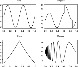
Figure 1: Trend functions used in the simulations: sine, JumpSine, “sharp” and Doppler.

4 Simulations

To study the potential benefits of data-adaptive wavelet estimation as outlined above, a simulation study was carried out with four different test functions $g$ (Figure 1) and a Gaussian $\operatorname{FARIMA}(0,d,0$) residual process $\xi_{i}$. Note that $\alpha=1-2d$. The test functions are:

• sine function: $g_{1}(t)=10\sin(4\uppi t);$

• JumpSine function: $g_{2}(t)=10\sin(4\uppi t)+\Delta\cdot I\{\frac{5}{8}<t<\frac{7}{8}\}$ $(\Delta>0);$

• “sharp” function: $g_{3}(t)=10[\exp(tI\{t<0.5\}+(1-t)I\{t>0.5\})-1];$

• Doppler function: $g_{4}(t)=10[t(1-t)]^{1/2}\sin[2\uppi(1+0.05)/(t+0.05)].$

The following methods are compared:

• Wavelet estimator with hard thresholding, $q$, $J$ as in Theorem 3 and

  $$\delta_{j}^{2}=\frac{4\mathrm{e}C_{\psi}^{2}N^{-1+\alpha}(\ln n)^{2}}{n^{\alpha}2^{(J+j)(1-\alpha)}}\qquad(q^{\ast}<j\leq q).$$

  Note that for the first three functions, Theorem 3(ii) applies, whereas for the Doppler function, derivatives are not bounded. Nevertheless, we carried out the simulations using a modified version of $C^{\ast}$ (see the remarks at the end of this section).

• Wavelet estimator with soft thresholding defined by

  $$\operatorname{sign}(\hat{d}_{jk})(|\hat{d}_{jk}|-\lambda_{n})I\{|\hat{d}_{jk}|>\lambda_{n}\}$$

  and minimax thresholds

  $$\lambda_{n}=(2\log n)^{1/2}$$

  (Johnstone and Silverman [33]).

• Kernel estimator with rectangular kernel $K(x)=\frac{1}{2}I\{x\in[-1,1]\}$ and asymptotically optimal bandwidth

  $$b_{\mathrm{opt}}=C_{\mathrm{opt}}n^{(2d-1)/(5-2d)},$$

  where

  $$C_{\mathrm{opt}} = \biggl{(}\frac{9(1-2d)\beta(d)C_{f}}{I(g^{\prime\prime})}\biggr{)}^{1/(5-2d)},$$

  $$\beta(d) = \frac{2^{2d}\Gamma(1-2d)\sin(\uppi d)}{d(2d+1)}$$

  (see, e.g., Hall and Hart [28], Beran and Feng [7]).

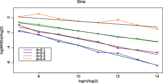
Figure 2: Simulated values of the mean integrated squared error, $\mathit{MISE}_{\mathrm{sim}}$, for different values of the fractional parameter $d$, plotted against the sample size ($n=2^{7},2^{8},\ldots,2^{13}$) on log–log scale (base 2 logarithms). The results are based on $400$ simulations of model (1) with the sine trend function and $\operatorname{FARIMA}(0,d,0$) residuals with $d=0.1,0.2,0.3,0.4.$ The estimates are based on Theorem 3 and wavelet basis $s4$.

Table 1: Logarithms (base 2) of simulated values of the mean integrated squared error, $\log_{2}\mathit{MISE}_{\mathrm{sim}},$ as a function of $n$ and the wavelet bases s4, s6, s8 and s10, respectively. For comparison, $\log_{2}\mathit{MISE}_{\mathrm{theor}}$ obtained from the asymptotic formulas in Theorem 3 is also given. The results are based on $400$ simulations of a $\operatorname{FARIMA}(0,0.2,0)$ model with trend function $g_{1}(t)=10\sin(4\uppi t)$

$n$	Simulation ‘s4’	Theor. ‘s4’	Simulation ‘s6’	Theor. ‘s6’
00 128	0.516420047	0.408553554	0.251744659	0.332459614
00 256	0.263441364	0.294451230	0.214928924	0.222321976
00 512	0.217604044	0.219171771	0.112951872	0.149658234
1024	0.150284851	0.150545678	0.110547951	0.101718042
2048	0.109213215	0.100879757	0.079795806	0.070089311
4096	0.061483507	0.068112469	0.049441935	0.049222131
8192	0.050871673	0.046494121	0.030814609	0.035454926
16 384	0.040330363	0.032231330	0.020141994	0.026371959
$n$	Simulation ‘s8’	Theor. ‘s8’	Simulation ‘s10’	Theor. ‘s10’
00 128	0.251744659	0.290131091	0.348379471	0.251989178
00 256	0.214928924	0.193352318	0.20541786	0.174618829
00 512	0.112951872	0.129502140	0.158692616	0.123573436
1024	0.110547951	0.087376732	0.074319167	0.089896035
2048	0.079795806	0.059584328	0.061712354	0.065326166
4096	0.049441935	0.041248179	0.030175723	0.043107368
8192	0.030814609	0.029150833	0.027662929	0.028448428
16 384	0.020141994	0.021169561	0.020361623	0.018777135

Sine: Figure 2 shows reasonably good agreement between the simulated and theoretical MISE of the adaptive wavelet estimator with basis s4. Here, s4, s6$,\ldots$ denote Daubechies’ wavelets with $2,3,\dots$ vanishing moments, respectively (see Daubechies [17]). Table 1 illustrates the effect of using different basis functions for the case $d=0.2$. Irrespective of the wavelet basis (s4, s6, s8 or s10), the agreement between the simulated MISE and the theoretical formula is already very good for $n=256.$ However, since $g$ is infinitely continuously differentiable, the MISE can be reduced by using very smooth basis functions. This explains why the performance of s4 is considerably worse compared with s6, s8 and s10. Table 2 shows that, as expected, the mean squared error increases with increasing long memory (see also Figure 2). A comparison between minimax wavelet thresholding, the data-adaptive wavelet estimator and kernel smoothing is given in Figures 3 and 4. Since the sine function is well behaved, optimal kernel estimation is expected to perform well. The kernel estimator does indeed outperform the minimax procedure. In contrast, the MISE of the data-adaptive wavelet method is comparable to optimal kernel estimation. A typical sample path and the corresponding estimated trend functions are plotted in Figure 5. The minimax rule leads to a rather erratic function near local minima and maxima, whereas this is not the case for the other two methods.

Table 2: Simulated values of the MISE for different sample sizes and values of $d$. The results are based on $400$ simulations of model (1) with $\operatorname{FARIMA}(0,d,0)$ residuals, the sine trend function $g_{1}$ and the wavelet estimator based on Theorem 3 with wavelet basis s4

$n$	$d=0.1$	$d=0.2$	$d=0.3$	$d=0.4$
00128	0.284521469	0.516420047	0.661787865	1.104194018
00256	0.210694474	0.263441364	0.537558642	1.42979724
00512	0.110584545	0.217604044	0.403889173	0.927229839
1024	0.078905169	0.150284851	0.29832426	0.717419015
2048	0.041133887	0.109213215	0.228981208	0.64283222
4096	0.037871696	0.061483507	0.165045782	0.818104781
8192	0.021438157	0.050871673	0.1444763	0.505236717
16 384	0.012234701	0.040330363	0.11107171	0.351823994

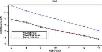
Figure 3: Simulated values of $\log_{2}\mathit{MISE}_{\mathrm{sim}}$ plotted against $\log n$ ($n=2^{7},2^{8},\ldots,2^{13}$) for trend estimates obtained by kernel smoothing, minimax soft threshold wavelet estimation and data-adaptive hard threshold wavelet estimation obtained from Theorem 3 (both with basis s4). The results are based on $400$ simulations of model (1) with the sine trend function and $\operatorname{FARIMA}(0,0.2,0)$ residuals.

Jumpsine: The simulated and asymptotic MISE for the Jumpsine function are compared in Table 3 for $d=0.2$ and jump sizes $\Delta=0.1,0.5,1,10,20$ and $50$. The agreement between the asymptotic and simulated MISE is reasonably good, in particular for small and very large values of $\Delta.$ Figure 6a shows a typical sample path with $d=0.3$ and fits obtained by the three methods. Figure 6b shows that, as expected from Theorem 3(ii), almost all non-zero coefficients belong to the father wavelet. The mother wavelet functions are useful for modeling the two jumps. Due to thresholding, almost all coefficients are eliminated except those near $t=5/8$ and $7/8$. Similar results were obtained for other values of $d.$ In comparison, the data-adaptive wavelet method shows the best performance (Figures 7 and 8), although the difference between the two wavelet methods is smaller under strong long memory. As expected, kernel estimation cannot compete with the wavelet approach.

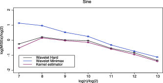
Figure 4: Simulated values of $\log_{2}\mathit{MISE}_{\mathrm{sim}}$ plotted against $\log n$ ($n=2^{7},2^{8},\ldots,2^{13}$) for trend estimates obtained by kernel smoothing, minimax soft threshold wavelet estimation and data-adaptive hard threshold wavelet estimation obtained from Theorem 3 (both with basis s4). The results are based on $400$ simulations of model (1) with the sine trend function and $\operatorname{FARIMA}(0,0.4,0)$ residuals.

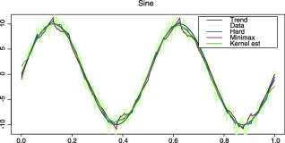
Figure 5: Simulated data with sine function plus $\operatorname{FARIMA}(0,0.3,0)$ process, and trend estimates obtained by optimal kernel smoothing, minimax soft thresholding wavelet estimation and data-adaptive hard threshold wavelet estimation according to Theorem 3 (both with basis s4).

=300pt $\Delta$ $n=2048$ $n=4096$ $n=8192$ 0.1 1.02984365 1.000066053 0.996328962 0.5 1.044736472 1.007194657 1.004583086 1 1.10352021 1.120497921 1.096100157 10 1.635074083 1.690840646 1.563330038 20 1.301618649 1.234763386 1.207770083 50 1.222581848 1.21888936 1.115174282

Table 3: $\mathit{MISE}_{\mathrm{sim}}/\mathit{MISE}_{\mathrm{theor}}$ for the JumpSine function and FARIMA(0, 0.2, 0) residuals, in dependence on the jump size $\Delta.$ The results are based on $400$ simulations and a thresholding estimate according to Theorem 3, with wavelet basis $s4$

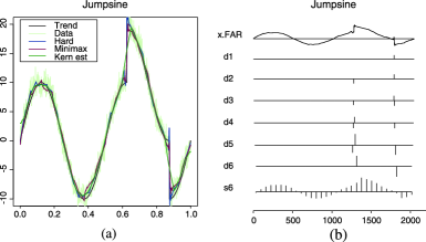
Figure 6: Simulated data (a) with JumpSine function plus $\operatorname{FARIMA}(0,0.3,0)$ process, and trend estimates obtained by kernel smoothing, minimax soft threshold wavelet estimation and data-adaptive hard threshold wavelet estimation obtained from Theorem 3 (both with basis s4); (b) shows the coefficients of the data-adaptive wavelet estimate.

Sharp: In distinct contrast to the JumpSine function, for the sharp function, the performance of the kernel estimator is comparable to the data-adaptive wavelet method (Figures 9 and 10), at least when the criterion is the MISE. With respect to the visual fit, as exemplified by Figure 11, the kernel method leads to oversmoothing of the edge in the middle.

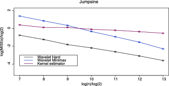
Figure 7: Simulated values of $\log_{2}\mathit{MISE}_{\mathrm{sim}}$ plotted against $\log n$ ($n=2^{7},2^{8},\ldots,2^{13}$) for trend estimates obtained by kernel smoothing, minimax soft threshold wavelet estimation and data-adaptive hard threshold wavelet estimation obtained from Theorem 3 (both with basis s4). The results are based on $400$ simulations of model (1) with the JumpSine trend function and $\operatorname{FARIMA}(0,0.2,0)$ residuals.

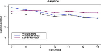
Figure 8: Simulated values of $\log_{2}\mathit{MISE}_{\mathrm{sim}}$ plotted against $\log n$ ($n=2^{7},2^{8},\ldots,2^{13}$) for trend estimates obtained by kernel smoothing, minimax soft threshold wavelet estimation and data-adaptive hard threshold wavelet estimation obtained from Theorem 3 (both with basis s4). The results are based on $400$ simulations of model (1) with the JumpSine trend function and $\operatorname{FARIMA}(0,0.4,0)$ residuals.

Doppler: For the Doppler function, Theorem 3 is not applicable and $J^{\ast}$ in equation (17) is not well defined. Nevertheless, it is interesting to see how well hard thresholding may work with a slight modification of (17). Specifically, consider

$$\tilde{J}^{\ast}=\biggl{\lfloor}\frac{\alpha}{2r+\alpha}\log_{2}n+\tilde{C}^{\ast}\bigl{(}r,\alpha,\psi,\phi,g^{(r)}\bigr{)}\biggr{\rfloor}+1,$$

where

$$\tilde{C}^{\ast}\bigl{(}r,\alpha,\psi,\phi,g^{(r)}\bigr{)}=\frac{1}{2r+\alpha}\log_{2}\biggl{[}\frac{\int_{0.1}^{0.95}\nu_{r}^{2}(g^{(r)}(t))^{2}\,\mathrm{d}t}{C_{\phi}^{2}(2^{\alpha}-1)(r!)^{2}}\biggr{]}-\log_{2}N.$$

Note that the only change compared to $C^{\ast}$ consists of bounding the integration limits away from $0$ and $1$. For moderate long memory with $d=0.2,$ the data-adaptive wavelet estimator still turns out to be the best (Figure 12). For strong long memory with $d=0.4$, the minimax approach appears to be slightly better for very long series (Figure 13). The relatively good performance of the minimax approach is expected because, in contrast to the data-adaptive estimator, the coarser levels of resolution are not favored a priori. This way, it is easier to catch the increasingly fast oscillations toward the left of the timescale. As expected, the kernel method does not work well. A typical example is shown in Figure 14.

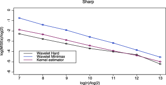
Figure 9: Simulated values of $\log_{2}\mathit{MISE}_{\mathrm{sim}}$ plotted against $\log n$ ($n=2^{7},2^{8},\ldots,2^{13}$) for trend estimates obtained by kernel smoothing, minimax soft threshold wavelet estimation and data-adaptive hard threshold wavelet estimation obtained from Theorem 3 (both with basis s4). The results are based on $400$ simulations of model (1) with the “sharp” trend function and $\operatorname{FARIMA}(0,0.2,0)$ residuals.

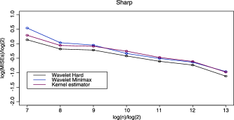
Figure 10: Simulated values of $\log_{2}\mathit{MISE}_{\mathrm{sim}}$ plotted against $\log n$ ($n=2^{7},2^{8},\ldots,2^{13}$) for trend estimates obtained by kernel smoothing, minimax soft threshold wavelet estimation and data-adaptive hard threshold wavelet estimation obtained from Theorem 3 (both with basis s4). The results are based on $400$ simulations of model (1) with the “sharp” trend function and $\operatorname{FARIMA}(0,0.4,0)$ residuals.

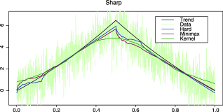
Figure 11: Simulated data with “sharp” function plus $\operatorname{FARIMA}(0,0.3,0)$ process, and trend estimates obtained by kernel smoothing, minimax soft threshold wavelet estimation and data-adaptive hard threshold wavelet estimation obtained from Theorem 3 (both with basis s4).

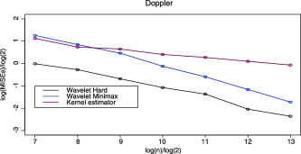
Figure 12: Simulated values of $\log_{2}\mathit{MISE}_{\mathrm{sim}}$ plotted against $\log n$ ($n=2^{7},2^{8},\ldots,2^{13}$) for trend estimates obtained by kernel smoothing, minimax soft threshold wavelet estimation and data-adaptive hard threshold wavelet estimation with $J=\tilde{J}^{*}$ and thresholds $\delta_{i}$ as in Theorem 3(ii) (both with basis s4). The results are based on $400$ simulations of model (1) with the Doppler trend function and $\operatorname{FARIMA}(0,0.2,0)$ residuals.

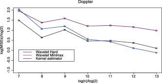
Figure 13: Simulated values of $\log_{2}\mathit{MISE}_{\mathrm{sim}}$ plotted against $\log n$ ($n=2^{7},2^{8},\ldots,2^{13}$) for trend estimates obtained by kernel smoothing, minimax soft threshold wavelet estimation and data-adaptive hard threshold wavelet estimation with $J=\tilde{J}^{*}$ and thresholds $\delta_{i}$ as in Theorem 3(ii) (both with basis s4). The results are based on $400$ simulations of model (1) with the Doppler trend function and $\operatorname{FARIMA}(0,0.4,0)$ residuals.

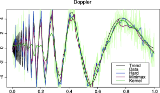
Figure 14: Simulated data with the Doppler function plus $\operatorname{FARIMA}(0,0.3,0)$ process, and trend estimates obtained by kernel smoothing, minimax soft threshold wavelet estimation and data-adaptive hard threshold wavelet estimation with $J=\tilde{J}^{*}$ and thresholds $\delta_{i}$ as in Theorem 3(ii) (both with basis s4).

5 Concluding remarks

In this paper, an approach to data-adaptive wavelet estimation of trend functions for long-memory time series models is proposed. The estimator can be understood as a combination of two components: a smoothing component consisting of a certain number of lower resolution levels where no thresholding is applied and a higher resolution component filtered by thresholding. The first component leads to good performance for smooth functions, whereas the second component is useful for modeling discontinuities. An open problem worth pursuing in future research is the question of how much more may be gained by further optimization with respect to fully flexible thresholds $\delta_{j}$.

Appendix: Proofs

In the proofs of Theorems 1, 2 and 3, $\phi$ and $\psi$ will be assumed to be piecewise differentiable. Analogous results (apart from some expressions in the remainder terms) can be obtained even if $\phi^{\prime}$ and $\psi^{\prime}$ do not exist anywhere, provided that both functions $\phi$ and $\psi$ satisfy a uniform Hölder condition with exponent $1/2$ (see (9)). The proofs are analogous, with the difference that instead of the rectangle rule (25), the mean value theorem is applied.

Proof of Theorem 1 Let

$$\mathit{MISE}=E\biggl{[}\int_{0}^{1}\bigl{(}g(t)-\hat{g}(t)\bigr{)}^{2}\,\mathrm{d}t\biggr{]}$$ (23)

denote the mean integrated square error. Combining (23) with (7) and (8), we have

$$\mathit{MISE}=E\Biggl{\{}\int_{0}^{1}\Biggl{[}\sum_{k=-N+1}^{N2^{J}-1}(s_{Jk}-\hat{s}_{Jk})\phi_{Jk}(t)$$

$$\hphantom{\mathit{MISE}=E\Biggl{\{}\int_{0}^{1}\Biggl{[}}{}+\sum_{j=0}^{q}\sum_{k=-N+1}^{N2^{J+j}-1}\bigl{(}d_{jk}-\hat{d}_{jk}I(|\hat{d}_{jk}|>\delta_{j})\bigr{)}\psi_{jk}(t)$$

$$\hphantom{\mathit{MISE}=E\Biggl{\{}\int_{0}^{1}\Biggl{[}}{}+\sum_{j=q+1}^{\infty}\sum_{k=-N+1}^{N2^{J+j}-1}d_{jk}\psi_{jk}\Biggr{]}^{2}\,\mathrm{d}t\Biggr{\}}.$$

Orthonormality of the basis in $L^{2}(\mathbb{R})$ implies that

$$\mathit{MISE} = E\Biggl{\{}\sum_{k=-N+1}^{N2^{J}-1}[\hat{s}_{Jk}-s_{Jk}]^{2}\Biggr{\}}$$

$${}+E\Biggl{\{}\sum_{j=0}^{q}\sum_{k=-N+1}^{N2^{J+j}-1}[\hat{d}_{jk}I(|\hat{d}_{jk}|>\delta_{j})-d_{jk}]^{2}\Biggr{\}}+\sum_{j=q+1}^{\infty}\sum_{k=-N+1}^{N2^{J+j}-1}d_{jk}^{2}$$

$$= \sum_{k=-N+1}^{N2^{J}-1}[E(\hat{s}_{Jk})-s_{Jk}]^{2}+\sum_{k=-N+1}^{N2^{J}-1}E\{[\hat{s}_{Jk}-E(\hat{s}_{Jk})]^{2}\}$$

$${}+\sum_{j=0}^{q}\sum_{k=-N+1}^{N2^{J+j}-1}\{E[(\hat{d}_{jk}-d_{jk})^{2}I(|\hat{d}_{jk}|>\delta_{j})]+E[d_{jk}^{2}I(|\hat{d}_{jk}|\leq\delta_{j})]\}$$

$${}+\sum_{j=q+1}^{\infty}\sum_{k=-N+1}^{N2^{J+j}-1}d_{jk}^{2}=\Lambda_{1}+\Lambda_{2}+\Lambda_{3}+\Lambda_{4}.$$

The proof then follows from Lemmas 1–6, given below.

Lemma 1.

Suppose that the first derivatives of $g$ and $\phi$ exist except for a finite number of points. Moreover, assume that $g^{\prime}$ and $\phi^{\prime}$ (where they exist) are piecewise continuous and bounded. Then,

$$\Lambda_{1}=\sum_{k=-N+1}^{N2^{J}-1}[E(\hat{s}_{Jk})-s_{Jk}]^{2}=\mathrm{O}(n^{-2}2^{2J}).$$

Proof.

For the expected value, we have

$$E(\hat{s}_{Jk}) = E\Biggl{(}\frac{1}{n}\sum_{i=1}^{n}Y_{i}\phi_{Jk}(t_{i})\Biggr{)}=\frac{N^{1/2}2^{J/2}}{n}\sum_{i=1}^{n}g\biggl{(}\frac{i}{n}\biggr{)}\phi\biggl{(}N2^{J}\frac{i}{n}-k\biggr{)}$$

$$= N^{1/2}2^{J/2}\sum_{i=1}^{n}\frac{1}{n}g\biggl{(}\frac{i}{n}\biggr{)}\phi\biggl{(}N2^{J}\frac{i}{n}-k\biggr{)}.$$

First, assume that $g$ and $\phi$ are continuously differentiable and recall the rectangle rule

$$\int_{a}^{b}f(t)\,\mathrm{d}t=\frac{b-a}{n}\sum_{i=0}^{n-1}f\biggl{(}a+i\frac{(b-a)}{n}\biggr{)}+\mathrm{O}\Biggl{(}\sum_{i=0}^{n-1}\sup_{t\in I_{i}}|f^{\prime}(t)|\cdot\frac{(b-a)^{2}}{n^{2}}\Biggr{)}$$ (25)

with $I_{i}=[a+i\frac{(b-a)}{n},a+(i+1)\frac{(b-a)}{n}]$. Noting that the support of $\phi(N2^{J}t-k)$ (as a function of $t$) is $[kN^{-1}2^{-J},(kN^{-1}+1)2^{-J}],$ we obtain

$$E(\hat{s}_{Jk})=N^{1/2}2^{J/2}\sum_{i=i_{1}(k)}^{i_{2}(k)}\frac{1}{n}g\biggl{(}\frac{i}{n}\biggr{)}\phi\biggl{(}N2^{J}\frac{i}{n}-k\biggr{)}$$

with

$$i_{1}(k)=nkN^{-1}2^{-J}$$

and

$$i_{2}(k)=n(kN^{-1}+1)2^{-J}.$$

Thus, the number of non-zero terms in the sum is $n2^{-J}+1$. This, together with the rectangle rule for $f(i/n)=g(i/n)\phi(N2^{J}i/n-k)$ (and integration limits $a=0$, $b=1$), implies that

$$E(\hat{s}_{Jk})=N^{1/2}2^{J/2}\int_{0}^{1}g(t)\phi(N2^{J}t-k)\,\mathrm{d}t+\mathrm{O}(n^{-1}2^{J/2})=s_{Jk}+\mathrm{O}(n^{-1}2^{J/2}).$$

Note that, here, the factor $2^{J}$ from the derivative of $\phi(N2^{J}t-k)$ is compensated by the fact that the number of non-zero terms in the sum is proportional to $2^{-J}$.

Now, assume, more generally, that $g^{\prime}$ and $\phi^{\prime}$ exist except for a finite number of points and, where they exist, that they are piecewise continuous and bounded. The result then follows by a piecewise application of the rectangle rule.

In summary, we have

$$E(\hat{s}_{Jk})-s_{Jk}=\mathrm{O}(n^{-1}2^{J/2}).$$

This implies that

$$\Lambda_{1}=\sum_{k=-N+1}^{N2^{J}-1}[E(\hat{s}_{Jk})-s_{Jk}]^{2}=\mathrm{O}\Biggl{(}\sum_{k=-N+1}^{N2^{J}-1}n^{-2}2^{J}\Biggr{)}=\mathrm{O}(n^{-2}2^{2J}),$$

which completes the proof. ∎

Lemma 2.

Suppose that the first derivative of $\phi$ exists on $[0,N]$ except for a finite number of points and, where $\phi^{\prime}$ exists, it is piecewise continuous and bounded. Let $J\geq 0$ and $-N+1\leq k\leq N2^{J}-1$. Then,

$$E\{[\hat{s}_{Jk}-E(\hat{s}_{Jk})]^{2}\}=C_{\phi}^{2}N^{-1+\alpha}n^{-\alpha}2^{-J(1-\alpha)}+\mathrm{O}(n^{-1})$$

and

$$\Lambda_{2}=\sum_{k=-N+1}^{N2^{J}-1}E\{[\hat{s}_{Jk}-E(\hat{s}_{Jk})]^{2}\}=C_{\phi}^{2}n^{-\alpha}N^{\alpha}2^{\alpha J}+\mathrm{O}(n^{-1}2^{J})+\mathrm{O}\bigl{(}n^{-\alpha}2^{-J(1-\alpha)}\bigr{)},$$

where $C_{\phi}$ is the constant in (11).

Proof.

First, assume that $\phi$ is continuously differentiable. Note that $C_{\phi}$ is a positive finite constant (see Li and Xiao [34]). We now consider the behavior of $E\{[\hat{s}_{Jk}-E(\hat{s}_{Jk})]^{2}\}$. We have

$$E\{[\hat{s}_{Jk}-E(\hat{s}_{Jk})]^{2}\}$$

$$\quad=E\Biggl{\{}\Biggl{[}\frac{1}{n}\sum_{i=1}^{n}\bigl{(}Y_{i}-E(Y_{i})\bigr{)}\phi_{Jk}(t_{i})\Biggr{]}^{2}\Biggr{\}}$$

$$\quad=E\Biggl{[}\Biggl{(}\frac{N^{1/2}2^{J/2}}{n}\sum_{i=1}^{n}\xi_{i}\phi\biggl{(}N2^{J}\frac{i}{n}-k\biggr{)}\Biggr{)}^{2}\Biggr{]}$$

$$\quad=Nn^{-2}2^{J}\sum_{i=1}^{n}\sum_{l=1}^{n}E(\xi_{i}\xi_{l})\phi\biggl{(}N2^{J}\frac{i}{n}-k\biggr{)}\phi\biggl{(}N2^{J}\frac{l}{n}-k\biggr{)}$$

$$\quad=Nn^{-2}2^{J}\sum_{i=nkN^{-1}2^{-J}}^{(1+kN^{-1})n2^{-J}}\sum_{l=nkN^{-1}2^{-J}}^{(1+kN^{-1})n2^{-J}}\gamma(l-i)\phi\biggl{(}N2^{J}\frac{i}{n}-k\biggr{)}\phi\biggl{(}N2^{J}\frac{l}{n}-k\biggr{)}$$

$$\quad=Nn^{-2}2^{J}\mathop{\sum_{i,l=nkN^{-1}2^{-J}}}_{i\neq l}^{(1+kN^{-1})n2^{-J}}\gamma(l-i)\phi\biggl{(}N2^{J}\frac{i}{n}-k\biggr{)}\phi\biggl{(}N2^{J}\frac{l}{n}-k\biggr{)}$$

$$\qquad{}+Nn^{-2}2^{J}\gamma(0)\sum_{i=nkN^{-1}2^{-J}}^{(1+kN^{-1})n2^{-J}}\phi^{2}\biggl{(}N2^{J}\frac{i}{n}-k\biggr{)}.$$

Equation (25) implies that

$$Nn^{-2}2^{J}\gamma(0)\sum_{i=nkN^{-1}2^{-J}}^{(1+kN^{-1})n2^{-J}}\phi^{2}\biggl{(}N2^{J}\frac{i}{n}-k\biggr{)}$$

$$\quad=n^{-1}\gamma(0)\Biggl{(}\frac{N}{n2^{-J}}\sum_{i=nkN^{-1}2^{-J}}^{(1+kN^{-1})n2^{-J}}\phi^{2}\biggl{(}N2^{J}\frac{i}{n}-k\biggr{)}\Biggr{)}$$

$$\quad=n^{-1}\gamma(0)\int_{0}^{N}\phi^{2}(t)\,\mathrm{d}t+\mathrm{o}(n^{-1}).$$

Due to (3), this is equal to

$$n^{-1}\gamma(0)+\mathrm{o}(n^{-1})=\mathrm{O}(n^{-1}).$$

Hence,

$$E\{[\hat{s}_{Jk}-E(\hat{s}_{Jk})]^{2}\}$$

$$\quad=Nn^{-2}2^{J}\mathop{\sum_{i,l=nkN^{-1}2^{-J}}}_{i\neq l}^{(1+kN^{-1})n2^{-J}}\gamma(l-i)\phi\biggl{(}N2^{J}\frac{i}{n}-k\biggr{)}\phi\biggl{(}N2^{J}\frac{l}{n}-k\biggr{)}+\mathrm{O}(n^{-1}).$$

Again using formula (2), we obtain, by arguments analogous to those in, for example, Taqqu [41],

$$E\{[\hat{s}_{Jk}-E(\hat{s}_{Jk})]^{2}\}$$

$$\quad\sim C_{\gamma}Nn^{-2}2^{J}\mathop{\sum_{i,l=nkN^{-1}2^{-J}}}_{i\neq l}^{(1+kN^{-1})n2^{-J}}|l-i|^{-\alpha}\phi\biggl{(}N2^{J}\frac{i}{n}-k\biggr{)}\phi\biggl{(}N2^{J}\frac{l}{n}-k\biggr{)}$$

$$\quad=C_{\gamma}N^{\alpha}n^{-1-\alpha}2^{\alpha J}\sum_{i=nkN^{-1}2^{-J}}^{(1+kN^{-1})n2^{-J}}\phi\biggl{(}N2^{J}\frac{i}{n}-k\biggr{)}\frac{N2^{J}}{n}$$

$$\quad\hphantom{=C_{\gamma}N^{\alpha}n^{-1-\alpha}2^{\alpha J}\sum_{i=nkN^{-1}2^{-J}}^{(1+kN^{-1})n2^{-J}}}{}\times\mathop{\sum_{l=nkN^{-1}2^{-J}}}_{l\neq i}^{(1+kN^{-1})n2^{-J}}\biggl{|}N2^{J}\frac{l}{n}-N2^{J}\frac{i}{n}\biggr{|}^{-\alpha}\phi\biggl{(}N2^{J}\frac{l}{n}-k\biggr{)}.$$

The function $f(x)=|x-(N2^{J}\frac{i}{n}-k)|^{-\alpha}\phi(x)$ is differentiable on $[0,N2^{J}\frac{i-1}{n}-k]\cup[N2^{J}\frac{i+1}{n}-k,N]$ for all fixed $i$ and $n$. Therefore, the rectangle rule implies that

$$\frac{N}{n2^{-J}}\mathop{\sum_{l=nkN^{-1}2^{-J}}}_{l\neq i}^{(1+kN^{-1})n2^{-J}}\biggl{|}N2^{J}\frac{l}{n}-N2^{J}\frac{i}{n}\biggr{|}^{-\alpha}\phi\biggl{(}N2^{J}\frac{l}{n}-k\biggr{)}$$

$$\quad=\frac{N}{n2^{-J}}\sum_{l=nkN^{-1}2^{-J}}^{i-1}\biggl{|}\biggl{(}N2^{J}\frac{l}{n}-k\biggr{)}-\biggl{(}N2^{J}\frac{i}{n}-k\biggr{)}\biggr{|}^{-\alpha}\phi\biggl{(}N2^{J}\frac{l}{n}-k\biggr{)}$$

$$\qquad{}+\frac{N}{n2^{-J}}\sum_{l=i+1}^{(1+kN^{-1})n2^{-J}}\biggl{|}\biggl{(}N2^{J}\frac{l}{n}-k\biggr{)}-\biggl{(}N2^{J}\frac{i}{n}-k\biggr{)}\biggr{|}^{-\alpha}\phi\biggl{(}N2^{J}\frac{l}{n}-k\biggr{)}$$

$$\quad=\int_{0}^{N2^{J}((i-1)/n)-k}\biggl{|}x-\biggl{(}N2^{J}\frac{i}{n}-k\biggr{)}\biggr{|}^{-\alpha}\phi(x)\,\mathrm{d}x$$

$$\qquad{}+\int_{N2^{J}((i+1)/n)-k}^{N}\biggl{|}x-\biggl{(}N2^{J}\frac{i}{n}-k\biggr{)}\biggr{|}^{-\alpha}\phi(x)\,\mathrm{d}x+K_{1,n}+K_{2,n},$$

where

$$K_{1,n}=\mathrm{O}\Biggl{(}\biggl{(}\frac{N}{n2^{-J}}\biggr{)}^{2}\sum_{l=nkN^{-1}2^{-J}}^{i-2}\sup_{x\in I_{l}(k)}\biggl{|}\frac{\mathrm{d}}{\mathrm{d}x}\biggl{(}\biggl{|}x-\biggl{(}N2^{J}\frac{i}{n}-k\biggr{)}\biggr{|}^{-\alpha}\phi(x)\biggr{)}\biggr{|}\Biggr{)}$$

with $I_{l}(k)=[N2^{J}l/n-k,N2^{J}(l+1)/n-k]$ and

$$K_{2,n} = \mathrm{O}\Biggl{(}\biggl{(}\frac{N}{n2^{-J}}\biggr{)}^{2}$$

$$\hphantom{\mathrm{O}\Biggl{(}}{}\times\sum_{l=i+1}^{(1+kN^{-1})n2^{-J}-1}\sup_{x\in I_{l}(k)}\biggl{|}\frac{\mathrm{d}}{\mathrm{d}x}\biggl{(}\biggl{|}x-\biggl{(}N2^{J}\frac{i}{n}-k\biggr{)}\biggr{|}^{-\alpha}\phi(x)\biggr{)}\biggr{|}\Biggr{)}.$$

Now,

$$\Biggl{|}\biggl{(}\frac{N}{n2^{-J}}\biggr{)}^{2}\sum_{l=nkN^{-1}2^{-J}}^{i-2}\sup_{x\in I_{l}(k)}\biggl{|}\frac{\mathrm{d}}{\mathrm{d}x}\biggl{(}\biggl{|}x-\biggl{(}N2^{J}\frac{i}{n}-k\biggr{)}\biggr{|}^{-\alpha}\phi(x)\biggr{)}\biggr{|}\Biggr{|}$$

$$\quad\leq\alpha N^{2}\max_{x\in[0,1]}\phi(x)\cdot\Biggl{|}n^{-2}2^{2J}\sum_{l=nkN^{-1}2^{-J}}^{i-2}\biggl{(}\biggl{(}N2^{J}\frac{i}{n}-k\biggr{)}-\biggl{(}N2^{J}\frac{l+1}{n}-k\biggr{)}\biggr{)}^{-1-\alpha}\Biggr{|}$$

$$\qquad{}+N^{2}\max_{x\in[0,1]}\phi^{\prime}(x)\cdot\Biggl{|}n^{-2}2^{2J}\sum_{l=nkN^{-1}2^{-J}}^{i-2}\biggl{(}\biggl{(}N2^{J}\frac{i}{n}-k\biggr{)}-\biggl{(}N2^{J}\frac{l+1}{n}-k\biggr{)}\biggr{)}^{-\alpha}\Biggr{|}$$

$$\quad\leq C_{1}n^{-(1-\alpha)}2^{J(1-\alpha)}\sum_{j=1}^{i-1-nkN^{-1}2^{-J}}j^{-1-\alpha}+C_{2}n^{-(2-\alpha)}2^{J(2-\alpha)}\sum_{j=1}^{i-1-nkN^{-1}2^{-J}}j^{-\alpha}$$

$$\quad\leq C_{1}n^{-(1-\alpha)}2^{J(1-\alpha)}\sum_{j=1}^{\infty}j^{-1-\alpha}+C_{2}n^{-(2-\alpha)}2^{J(2-\alpha)}\sum_{j=1}^{n2^{-J}}j^{-\alpha}$$

$$\quad\leq C_{1}n^{-(1-\alpha)}2^{J(1-\alpha)}\sum_{j=1}^{\infty}j^{-1-\alpha}+C_{2}^{\ast}n^{-1}2^{J}.$$

Thus,

$$K_{1,n}=\mathrm{O}\bigl{(}n^{-(1-\alpha)}2^{J(1-\alpha)}\bigr{)}.$$

By analogous arguments, we obtain

$$K_{2,n}=\mathrm{O}\bigl{(}n^{-(1-\alpha)}2^{J(1-\alpha)}\bigr{)}.$$

This implies that

$$E\{[\hat{s}_{Jk}-E(\hat{s}_{Jk})]^{2}\}$$

$$\quad=C_{\gamma}N^{\alpha}n^{-1-\alpha}2^{\alpha J}$$

$$\qquad{}\times\sum_{i=nkN^{-1}2^{-J}}^{(1+kN^{-1})n2^{-J}}\phi\biggl{(}N2^{J}\frac{i}{n}-k\biggr{)}\biggl{(}\int_{0}^{N2^{J}((i-1)/n)-k}\biggl{|}x-\biggl{(}N2^{J}\frac{i}{n}-k\biggr{)}\biggr{|}^{-\alpha}\phi(x)\,\mathrm{d}x$$

$$\qquad\hphantom{{}\times\sum_{i=nkN^{-1}2^{-J}}^{(1+kN^{-1})n2^{-J}}\phi\biggl{(}N2^{J}\frac{i}{n}-k\biggr{)}\biggl{(}}{}+\int_{N2^{J}((i+1)/n)-k}^{N}\biggl{|}x-\biggl{(}N2^{J}\frac{i}{n}-k\biggr{)}\biggr{|}^{-\alpha}\phi(x)\,\mathrm{d}x$$

$$\qquad\hphantom{{}\times\sum_{i=nkN^{-1}2^{-J}}^{(1+kN^{-1})n2^{-J}}\phi\biggl{(}N2^{J}\frac{i}{n}-k\biggr{)}\biggl{(}}{}+\mathrm{O}\bigl{(}n^{-(1-\alpha)}2^{J(1-\alpha)}\bigr{)}\biggr{)}+\mathrm{O}(n^{-1})$$

$$\quad=C_{\gamma}N^{\alpha}n^{-1-\alpha}2^{\alpha J}\sum_{i=nkN^{-1}2^{-J}}^{(1+kN^{-1})n2^{-J}}\phi\biggl{(}N2^{J}\frac{i}{n}-k\biggr{)}$$

$$\quad\hphantom{=C_{\gamma}N^{\alpha}n^{-1-\alpha}2^{\alpha J}\sum_{i=nkN^{-1}2^{-J}}^{(1+kN^{-1})n2^{-J}}}{}\times\int_{0}^{N2^{J}((i-1)/n)-k}\biggl{|}x-\biggl{(}N2^{J}\frac{i}{n}-k\biggr{)}\biggr{|}^{-\alpha}\phi(x)\,\mathrm{d}x$$

$$\qquad{}+C_{\gamma}N^{\alpha}n^{-1-\alpha}2^{\alpha J}\sum_{i=nkN^{-1}2^{-J}}^{(1+kN^{-1})n2^{-J}}\phi\biggl{(}N2^{J}\frac{i}{n}-k\biggr{)}$$

$$\qquad\hphantom{{}+C_{\gamma}N^{\alpha}n^{-1-\alpha}2^{\alpha J}\sum_{i=nkN^{-1}2^{-J}}^{(1+kN^{-1})n2^{-J}}}{}\times\int_{N2^{J}((i+1)/n)-k}^{N}\biggl{|}x-\biggl{(}N2^{J}\frac{i}{n}-k\biggr{)}\biggr{|}^{-\alpha}\phi(x)\,\mathrm{d}x$$

$$\qquad{}+\mathrm{O}(n^{-1})=A_{1}+A_{2}+\mathrm{O}(n^{-1}).$$

Again using (25), we obtain, by arguments analogous to those used above,

$$A_{1}=C_{\gamma}N^{-1+\alpha}n^{-\alpha}2^{-J(1-\alpha)}\int_{0}^{N}\!\!\!\int_{0}^{y-N2^{J}(1/n)}|x-y|^{-\alpha}\phi(x)\phi(y)\,\mathrm{d}x\,\mathrm{d}y+\mathrm{O}(n^{-1})$$

and

$$A_{2}=C_{\gamma}N^{-1+\alpha}n^{-\alpha}2^{-J(1-\alpha)}\int_{0}^{N}\!\!\!\int_{y+N2^{J}(1/n)}^{N}|x-y|^{-\alpha}\phi(x)\phi(y)\,\mathrm{d}x\,\mathrm{d}y+\mathrm{O}(n^{-1}).$$

Noting that

$$\int_{y-N2^{J}(1/n)}^{y+N2^{J}(1/n)}\!|x\,{-}\,y|^{-\alpha}\phi(x)\phi(y)\,\mathrm{d}x\,{\leq}\,2\max_{x\in[0,N]}(\phi^{2}(x))\,{\cdot}\,\int_{0}^{N2^{J}n^{-1}}\!z^{-\alpha}\,\mathrm{d}y\,{=}\,\mathrm{O}\bigl{(}n^{-(1-\alpha)}2^{J(1-\alpha)}\bigr{)},$$

we obtain

$$\int_{0}^{N}\!\!\!\int_{y-N2^{J}(1/n)}^{y+N2^{J}(1/n)}|x-y|^{-\alpha}\phi(x)\phi(y)\,\mathrm{d}x\,\mathrm{d}y=\mathrm{O}\bigl{(}n^{-(1-\alpha)}2^{J(1-\alpha)}\bigr{)}$$

and

$$E\{[\hat{s}_{Jk}-E(\hat{s}_{Jk})]^{2}\} = C_{\gamma}N^{-1+\alpha}n^{-\alpha}2^{-J(1-\alpha)}\int_{0}^{N}\!\!\!\int_{0}^{N}|x-y|^{-\alpha}\phi(x)\phi(y)\,\mathrm{d}x\,\mathrm{d}y+\mathrm{O}(n^{-1})$$

$$= C_{\phi}^{2}N^{-1+\alpha}n^{-\alpha}2^{-J(1-\alpha)}+\mathrm{O}(n^{-1}),$$

where $C_{\phi}$ is the constant in (11). Hence,

$$\Lambda_{2} = \sum_{k=-N+1}^{N2^{J}-1}E\{[\hat{s}_{Jk}-E(\hat{s}_{Jk})]^{2}\}=\sum_{k=-N+1}^{N2^{J}-1}\bigl{(}C_{\phi}^{2}N^{-1+\alpha}n^{-\alpha}2^{-J(1-\alpha)}+\mathrm{O}(n^{-1})\bigr{)}$$

$$= C_{\phi}^{2}n^{-\alpha}N^{\alpha}2^{\alpha J}+\mathrm{O}(n^{-1}2^{J})+\mathrm{O}\bigl{(}n^{-\alpha}2^{-J(1-\alpha)}\bigr{)}.$$

In the general case where $\phi^{\prime}$ exists except for a finite number of points and, where it exists, it is piecewise continuous and bounded, the result follows by a piecewise application of the rectangle rule. ∎

Lemma 3.

Suppose that the first derivative of $\psi$ exists on $[0,N]$ except for a finite number of points and, where $\psi^{\prime}$ exists, it is piecewise continuous and bounded. Let $J\geq 0$, $j\geq 0$ and $-N+1\leq k\leq N2^{J+j}-1$. Then

$$\sigma_{j}^{2} = E\{[\hat{d}_{jk}-E(\hat{d}_{jk})]^{2}\}$$

$$= C_{\psi}^{2}N^{-1+\alpha}n^{-\alpha}2^{-(J+j)(1-\alpha)}+\mathrm{O}(n^{-1}),$$

where $C_{\psi}$ is the constant in (12).

Proof.

Noting that

$$E\{[\hat{d}_{jk}-E(\hat{d}_{jk})]^{2}\}=E\Biggl{\{}\Biggl{[}\frac{N^{1/2}2^{(J+j)/2}}{n}\sum_{i=1}^{n}\xi_{i}\psi\biggl{(}N2^{J+j}\frac{i}{n}-k\biggr{)}\Biggr{]}^{2}\Biggr{\}},$$

the proof is analogous to the proof of Lemma 2, with the difference being that $\psi$ is used instead of $\phi$ and $J$ is replaced by $J+j$. ∎

Lemma 4.

Suppose that the first $r$ derivatives of $g$ exist and are continuous on $[0,1]$. Then, for all $j\geq 0$ and $0\leq k\leq N2^{J+j}-1$,

$$d_{jk} = \frac{\nu_{r}}{r!}g^{(r)}\bigl{(}kN^{-1}2^{-(J+j)}\bigr{)}N^{-(2r+1)/2}2^{-((2r+1)/2)(J+j)}$$

$${}+\mathrm{o}\bigl{(}2^{-((2r+1)/2)(J+j)}\bigr{)},$$

where $\nu_{r}$ is the $r$th moment of $\psi$ (see (6)). Together with the assumptions of Lemma 3, this yields that

$$E(\hat{d}_{jk})-d_{jk}=\mathrm{O}\bigl{(}n^{-1}2^{(J+j)/2}\bigr{)}.$$

Proof.

Note that

$$d_{jk} = N^{1/2}2^{(J+j)/2}\int_{0}^{1}g(t)\psi(N2^{J+j}t-k)\,\mathrm{d}t$$

$$= N^{1/2}2^{(J+j)/2}\int_{kN^{-1}2^{-(J+j)}}^{(1+kN^{-1})2^{-(J+j)}}g\bigl{(}N^{-1}2^{-(J+j)}[N2^{J+j}t-k+k]\bigr{)}\psi(N2^{J+j}t-k)\,\mathrm{d}t$$

$$= N^{-1/2}2^{-(J+j)/2}\int_{0}^{N}g\bigl{(}N^{-1}2^{-(J+j)}(y+k)\bigr{)}\psi(y)\,\mathrm{d}y.$$

Since $g$ is $r$-times continuously differentiable, the local Taylor expansion (see, e.g., Zorich [46], pages 225–226) of $g$ yields

$$d_{jk} = N^{-1/2}2^{-(J+j)/2}\int_{0}^{N}\psi(y)\biggl{[}g\bigl{(}kN^{-1}2^{-(J+j)}\bigr{)}+N^{-1}2^{-(J+j)}g^{\prime}\bigl{(}kN^{-1}2^{-(J+j)}\bigr{)}y$$

$$\hphantom{N^{-1/2}2^{-(J+j)/2}\int_{0}^{N}\psi(y)\biggl{[}}{}+\cdots+\frac{N^{-r}2^{-r(J+j)}}{r!}g^{(r)}\bigl{(}kN^{-1}2^{-(J+j)}\bigr{)}y^{r}\biggr{]}\,\mathrm{d}y$$

$${}+\mathrm{o}\bigl{(}2^{-((2r+1)/2)(J+j)}\bigr{)}.$$

The moment conditions (5) and (6) then imply that

$$d_{jk} \!=\! \frac{1}{r!}g^{(r)}\bigl{(}kN^{-1}2^{-(J+j)}\bigr{)}N^{-(2r+1)/2}2^{-((2r+1)/2)(J+j)}\!\!\int_{0}^{N}\!y^{r}\psi(y)\,\mathrm{d}y\,{+}\,\mathrm{o}\bigl{(}2^{-((2r+1)/2)(J+j)}\bigr{)}$$

$$\!=\! \frac{\nu_{r}}{r!}g^{(r)}\bigl{(}kN^{-1}2^{-(J+j)}\bigr{)}N^{-(2r+1)/2}2^{-((2r+1)/2)(J+j)}\,{+}\,\mathrm{o}\bigl{(}2^{-((2r+1)/2)(J+j)}\bigr{)}.$$

For $E(\hat{d}_{jk}),$ we have

$$E(\hat{d}_{jk}) = \frac{1}{n}\sum_{i=1}^{n}E[Y_{i}\psi_{jk}(t_{i})]$$

$$= N^{1/2}2^{(J+j)/2}\sum_{i=1}^{n}n^{-1}g\biggl{(}\frac{i}{n}\biggr{)}\psi\biggl{(}N2^{J+j}\frac{i}{n}-k\biggr{)}.$$

Again using the same arguments as in Lemma 1 for $E(\hat{s}_{Jk})$, we obtain that

$$E(\hat{d}_{jk})=d_{jk}+\mathrm{O}\bigl{(}n^{-1}2^{(J+j)/2}\bigr{)}.$$

∎

Lemma 5.

Under the assumptions of Lemma 4,

$$\Lambda_{4}=\frac{1}{(r!)^{2}}\frac{1}{2^{2r}-1}N^{-2r}2^{-2r(J+q)}\int_{0}^{1}\nu_{r}^{2}\bigl{(}g^{(r)}(t)\bigr{)}^{2}\,\mathrm{d}t+\mathrm{o}\bigl{(}2^{-2r(J+q)}\bigr{)}.$$

Proof.

Using (Appendix: Proofs), we have

$$\Lambda_{4} = \sum_{j=q+1}^{\infty}\sum_{k=-N+1}^{N2^{J+j}-1}d_{jk}^{2}$$

$$= \sum_{j=q+1}^{\infty}\sum_{k=-N+1}^{N2^{J+j}-1}\biggl{[}\frac{\nu_{r}}{r!}g^{(r)}\bigl{(}kN^{-1}2^{-(J+j)}\bigr{)}\biggr{]}^{2}N^{-(2r+1)}2^{-(2r+1)(J+j)}+\mathrm{o}\bigl{(}2^{-(2r+1)(J+j)}\bigr{)}.$$

Note that the continuity of $g^{(r)}$ implies convergence of the Riemann sum. Hence, $\Lambda_{4}$ is equal to

$$\frac{1}{(r!)^{2}}\sum_{j=q+1}^{\infty}N^{-2r}2^{-2r(J+j)}\biggl{\{}\int_{0}^{1}\nu_{r}^{2}\bigl{(}g^{(r)}(t)\bigr{)}^{2}\,\mathrm{d}t+\mathrm{o}(1)\biggr{\}}+\mathrm{o}\bigl{(}2^{-2r(J+q)}\bigr{)}$$

$$\quad=\frac{1}{(r!)^{2}}\frac{1}{2^{2r}-1}N^{-2r}2^{-2r(J+q)}\int_{0}^{1}\nu_{r}^{2}\bigl{(}g^{(r)}(t)\bigr{)}^{2}\,\mathrm{d}t+\mathrm{o}\bigl{(}2^{-2r(J+q)}\bigr{)}.$$

∎

Lemma 6.

Let

$$\hat{q}=\log_{2}n^{\alpha/(2r+\alpha)}+\frac{1}{2r+\alpha}\log_{2}\biggl{(}\frac{\nu_{r}^{2}}{(r!)^{2}C_{\psi}^{2}N^{2r+\alpha}}\max_{t\in[0,1]}\bigl{[}g^{(r)}(t)\bigr{]}^{2}\biggr{)}-J+1$$ (27)

and

$$\lambda_{jk}=E[(\hat{d}_{jk}-d_{jk})^{2}I(|\hat{d}_{jk}|>\delta_{j})]+E[d_{jk}^{2}I(|\hat{d}_{jk}|\leq\delta_{j})].$$

Under the assumptions of Lemmas 3 and 4, the following then holds: If $q>\hat{q}$, then for all $j$ with $\hat{q}<j<\frac{2+\alpha}{4r+2+\alpha}\log_{2}n-J$, we have

$$\min_{\delta_{j}}\lambda_{jk}=d_{jk}^{2}+\mathrm{O}\bigl{(}2^{\alpha(J+j)/2}n^{-(1+\alpha/2)}\bigr{)}.$$

Proof.

Defining $S_{0}=2^{-(2r+\alpha)}C_{\psi}^{2}N^{-1+\alpha}n^{-\alpha}2^{-(J+j)(1-\alpha)}$ and taking into account Lemma 3, we have $S_{1,j}=2^{-(2r+\alpha)}\sigma_{j}^{2}S_{0}^{-1}=1+r_{1,j}$ with $|r_{1,j}|\leq r_{1}=\mathrm{o}(1)$ for all $j\geq\hat{q}$. Moreover, Lemma 4 implies that

$$S_{2,jk} = d_{jk}^{2}S_{0}^{-1}=\frac{\nu_{r}^{2}}{(r!)^{2}C_{\psi}^{2}N^{2r+\alpha}}\bigl{[}g^{(r)}\bigl{(}kN^{-1}2^{-(J+j)}\bigr{)}\bigr{]}^{2}2^{-(2r+\alpha)(J+j-1)}n^{\alpha}+r_{2,jk}$$

$$\leq \frac{\nu_{r}^{2}}{(r!)^{2}C_{\psi}^{2}N^{2r+\alpha}}\max_{t\in[0,1]}\bigl{[}g^{(r)}(t)\bigr{]}^{2}n^{\alpha}\max_{j>\hat{q}}\bigl{\{}2^{-(2r+\alpha)(J+j-1)}\bigr{\}}+r_{2}$$

with $r_{2}=\mathrm{o}(1)$ independent of $j$ and $k$. Using (27), we obtain

$$S_{2,jk}\leq 2^{-(2r+\alpha)}+r_{2}\leq 1+r_{1}=S_{1,j}$$

for $j>\hat{q}$ and $n$ large enough, which implies that

$$\sigma_{j}\geq 2^{r+\alpha/2}\max_{k}|d_{jk}|.$$ (28)

The mean squared error $\lambda_{jk}$ can be written as

$$\lambda_{jk} = E[(\hat{d}_{jk}-d_{jk})^{2}I(|\hat{d}_{jk}|>\delta_{j})]+E[d_{jk}^{2}I(|\hat{d}_{jk}|\leq\delta_{j})]$$

$$= \frac{1}{\sqrt{2\uppi}\sigma_{j}}\int_{|t|>\delta_{j}}\!(t-d_{jk})^{2}\mathrm{e}^{-(1/(2\sigma_{j}^{2}))(t-E(\hat{d}_{jk}))^{2}}\,\mathrm{d}t+d_{jk}^{2}\frac{1}{\sqrt{2\uppi}\sigma_{j}}\int_{|t|<\delta_{j}}\!\mathrm{e}^{-(t-E(\hat{d}_{jk}))^{2}/(2\sigma_{j}^{2})}\,\mathrm{d}t$$

$$= A_{1}+A_{2}.$$

We approximate $A_{1}$ and $A_{2}$ separately. Taylor expansion of $A_{1}$ with respect to $E(\hat{d}_{jk})$ in the neighborhood of $d_{jk}$ yields

$$A_{1} = \frac{1}{\sqrt{2\uppi}\sigma_{j}}\int_{|t|>\delta_{j}}(t-d_{jk})^{2}\mathrm{e}^{-(1/(2\sigma_{j}^{2}))(t-E(\hat{d}_{jk}))^{2}}\,\mathrm{d}t$$

$$= \frac{1}{\sqrt{2\uppi}\sigma_{j}}\int_{|t|>\delta_{j}}(t-d_{jk})^{2}\mathrm{e}^{-(1/(2\sigma_{j}^{2}))(t-d_{jk})^{2}}\,\mathrm{d}t$$

$${}+\frac{E(\hat{d}_{jk})-d_{jk}}{\sqrt{2\uppi}\sigma_{j}}\int_{|t|>\delta_{j}}\frac{(t-d_{jk})^{3}}{\sigma_{j}^{2}}\mathrm{e}^{-(1/(2\sigma_{j}^{2}))(t-d_{jk})^{2}}\,\mathrm{d}t$$

$${}+\mathrm{O}\biggl{(}\frac{[E(\hat{d}_{jk})-d_{jk}]^{2}}{\sigma_{j}}\int_{|t|>\delta_{j}}\biggl{(}\frac{(t-d_{jk})^{4}}{\sigma_{j}^{4}}-\frac{(t-d_{jk})^{2}}{\sigma_{j}^{2}}\biggr{)}\mathrm{e}^{-(1/(2\sigma_{j}^{2}))(t-d_{jk})^{2}}\,\mathrm{d}t\biggr{)}.$$

If $d_{jk}\neq 0$, then Lemmas 3 and 4 imply that

$$\frac{E(\hat{d}_{jk})-d_{jk}}{\sigma_{j}}\int_{|t|>\delta_{j}}\frac{(t-d_{jk})^{3}}{\sigma_{j}^{2}}\mathrm{e}^{-(1/(2\sigma_{j}^{2}))(t-d_{jk})^{2}}\,\mathrm{d}t$$

$$\quad=\sigma_{j}[E(\hat{d}_{jk})-d_{jk}]\int_{|t|>\delta_{j}/\sigma_{j}}\biggl{(}t-\frac{d_{jk}}{\sigma_{j}}\biggr{)}^{3}\mathrm{e}^{-1/2(t-d_{jk}/\sigma_{j})^{2}}\,\mathrm{d}t$$ (29)

$$\quad=\mathrm{O}\bigl{(}n^{-\alpha/2}2^{-(J+j)(1-\alpha)/2}\cdot n^{-1}2^{(J+j)/2}\bigr{)}=\mathrm{O}\bigl{(}2^{\alpha(J+j)/2}n^{-(1+\alpha/2)}\bigr{)}.$$

If $d_{jk}=0$, then

$$\frac{E(\hat{d}_{jk})-d_{jk}}{\sigma_{j}}\int_{|t|>\delta_{j}}\frac{(t-d_{jk})^{3}}{\sigma_{j}^{2}}\mathrm{e}^{-(1/(2\sigma_{j}^{2}))(t-d_{jk})^{2}}\,\mathrm{d}t=0$$

and

$$\frac{[E(\hat{d}_{jk})-d_{jk}]^{2}}{\sigma_{j}}\int_{|t|>\delta_{j}}\biggl{(}\frac{(t-d_{jk})^{4}}{\sigma_{j}^{4}}-\frac{(t-d_{jk})^{2}}{\sigma_{j}^{2}}\biggr{)}\mathrm{e}^{-(1/(2\sigma_{j}^{2}))(t-d_{jk})^{2}}\,\mathrm{d}t$$

$$\quad=[E(\hat{d}_{jk})-d_{jk}]^{2}\int_{|t|>\delta_{j}/\sigma_{j}}\biggl{(}\biggl{(}t-\frac{d_{jk}}{\sigma_{j}}\biggr{)}^{4}-\biggl{(}t-\frac{d_{jk}}{\sigma_{j}}\biggr{)}^{2}\biggr{)}\mathrm{e}^{-(1/2)(t-d_{jk}/\sigma_{j})^{2}}\,\mathrm{d}t$$ (30)

$$\quad=\mathrm{O}(n^{-2}2^{J+j}).$$

The condition $j+J<\frac{2+\alpha}{4r+2+\alpha}\log_{2}n$ implies that ${n}^{-2}2^{J+j}=\mathrm{o}(2^{(\alpha/2)(J+j)}n^{-(1+\alpha/2)})$ so that

$$A_{1}=\frac{1}{\sqrt{2\uppi}\sigma_{j}}\int_{|t|>\delta_{j}}(t-d_{jk})^{2}\mathrm{e}^{(-1/(2\sigma_{j}^{2}))(t-d_{jk})^{2}}\,\mathrm{d}t+\mathrm{O}\bigl{(}2^{\alpha(J+j)/2}n^{-(1+\alpha/2)}\bigr{)}.$$ (31)

By analogous arguments, we have, for $d_{jk}\neq 0$,

$$A_{2} = d_{jk}^{2}\frac{1}{\sqrt{2\uppi}\sigma_{j}}\int_{|t|<\delta_{j}}\mathrm{e}^{-(t-E(\hat{d}_{jk}))^{2}/(2\sigma_{j}^{2})}\,\mathrm{d}t$$

$$= d_{jk}^{2}\frac{1}{\sqrt{2\uppi}\sigma_{j}}\int_{|t|<\delta_{j}}\mathrm{e}^{-(t-d_{jk})^{2}/(2\sigma_{j}^{2})}\,\mathrm{d}t$$

$${}+\mathrm{O}\biggl{(}\frac{d_{jk}^{2}[E(\hat{d}_{jk})-d_{jk}]}{\sigma_{j}}\int_{|t|<\delta_{j}}\frac{(t-d_{jk})}{\sigma_{j}^{2}}\mathrm{e}^{-(t-d_{jk})^{2}/(2\sigma_{j}^{2})}\,\mathrm{d}t\biggr{)}$$

with

$$\frac{d_{jk}^{2}[E(\hat{d}_{jk})-d_{jk}]}{\sigma_{j}}\int_{|t|<\delta_{j}}\frac{(t-d_{jk})}{\sigma_{j}^{2}}\mathrm{e}^{-(t-d_{jk})^{2}/(2\sigma_{j}^{2})}\,\mathrm{d}t$$

$$\quad=\frac{d_{jk}^{2}[E(\hat{d}_{jk})-d_{jk}]}{\sigma_{j}}\int_{|t|<\delta_{j}/\sigma_{j}}\biggl{(}t-\frac{d_{jk}}{\sigma_{j}}\biggr{)}\mathrm{e}^{-(1/2)(t-d_{jk}/\sigma_{j})^{2}}\,\mathrm{d}t$$

(32)

$$\quad=\mathrm{O}\bigl{(}2^{-(2r+1)(J+j)}\cdot n^{-1}2^{(J+j)/2}\cdot n^{\alpha/2}2^{(J+j)(1-\alpha)/2}\bigr{)}$$

$$\quad=\mathrm{O}\bigl{(}n^{-(1-\alpha/2)}2^{-(2r+\alpha/2)(J+j)}\bigr{)}.$$

For $d_{jk}=0$, we have

$$A_{2}=d_{jk}^{2}\frac{1}{\sqrt{2\uppi}\sigma_{j}}\int_{|t|<\delta_{j}}\mathrm{e}^{-(t-E(\hat{d}_{jk}))^{2}/(2\sigma_{j}^{2})}\,\mathrm{d}t=0.$$

In summary, we have derived the approximation,

$$\lambda_{jk} = A_{1}+A_{2}$$

$$= \sigma_{j}^{2}\frac{1}{\sqrt{2\uppi}}\int_{|t|>\delta_{j}/\sigma_{j}}\biggl{(}t-\frac{d_{jk}}{\sigma_{j}}\biggr{)}^{2}\mathrm{e}^{-(1/2)(t-d_{jk}/\sigma_{j})^{2}}\,\mathrm{d}t$$

$${}+d_{jk}^{2}\frac{1}{\sqrt{2\uppi}}\int_{|t|<\delta_{j}/\sigma_{j}}\mathrm{e}^{-(1/2)(t-d_{jk}/\sigma_{j})^{2}}\,\mathrm{d}t$$

$${}+\mathrm{O}\bigl{(}2^{\alpha(J+j)/2}n^{-(1+\alpha/2)}\bigr{)}+\mathrm{O}\bigl{(}n^{-(1-\alpha/2)}2^{-(2r+\alpha/2)(J+j)}\bigr{)}$$

with uniformly bounded error terms (see (Proof.), (Proof.) and (Proof.)). It is then sufficient to show that for all $k$ and all $j$ with $\hat{q}<j<\frac{2+\alpha}{4r+2+\alpha}\log_{2}n-J,$ we have

$$\min_{\delta_{j}}\hat{\lambda}_{jk}=d_{jk}^{2},$$

where

$$\hat{\lambda}_{jk} = \sigma_{j}^{2}\frac{1}{\sqrt{2\uppi}}\int_{|t|>\delta_{j}/\sigma_{j}}\biggl{(}t-\frac{d_{jk}}{\sigma_{j}}\biggr{)}^{2}\mathrm{e}^{-(1/2)(t-d_{jk}/\sigma_{j})^{2}}\,\mathrm{d}t$$

$${}+d_{jk}^{2}\frac{1}{\sqrt{2\uppi}}\int_{|t|<\delta_{j}/\sigma_{j}}\mathrm{e}^{-(1/2)(t-d_{jk}/\sigma_{j})^{2}}\,\mathrm{d}t.$$

In the following, we distinguish two cases: $\delta_{j}\leq\sigma_{j}$ and $\delta_{j}>\sigma_{j}$.

At first, let $\delta_{j}\leq\sigma_{j}$. Recall that $\sigma_{j}\geq 2^{r+\alpha/2}d_{jk}$ for all $k$ (see (28)). Then,

$$\frac{1}{\sqrt{2\uppi}}\int_{|t|\geq\delta_{j}/\sigma_{j}}\biggl{(}t-d_{jk}/\sigma_{j}\biggr{)}^{2}\mathrm{e}^{-(1/2)(t-d_{jk}/\sigma_{j})^{2}}\,\mathrm{d}t$$

$$\quad\geq\min_{0\leq x\leq 2^{-(r+\alpha/2)}}\frac{1}{\sqrt{2\uppi}}\int_{|t|\geq 1}(t-x)^{2}\mathrm{e}^{-(1/2)(t-x)^{2}}\,\mathrm{d}t$$

$$\quad\geq\min_{0\leq x\leq 2^{-1}}\frac{1}{\sqrt{2\uppi}}\int_{|t|\geq 1}(t-x)^{2}\mathrm{e}^{-(1/2)(t-x)^{2}}\,\mathrm{d}t>0.57.$$

Also, note that

$$\frac{1}{\sqrt{2\uppi}}\int_{|t|<\delta_{j}/\sigma_{j}}\mathrm{e}^{-(1/2)(t-d_{jk}/\sigma_{j})^{2}}\,\mathrm{d}t\geq 0.$$

These two inequalities and (Proof.) imply that for all $j>\hat{q}$,

$$\inf_{\delta_{j}\leq\sigma_{j}}\hat{\lambda}_{jk} = \inf_{\delta_{j}\leq\sigma_{j}}\biggl{\{}\sigma_{j}^{2}\frac{1}{\sqrt{2\uppi}}\int_{|t|>\delta_{j}/\sigma_{j}}\biggl{(}t-\frac{d_{jk}}{\sigma_{j}}\biggr{)}^{2}\mathrm{e}^{-(1/2)(t-d_{jk}/\sigma_{j})^{2}}\,\mathrm{d}t$$

$$\hphantom{\inf_{\delta_{j}\leq\sigma_{j}}\biggl{\{}}{}+d_{jk}^{2}\frac{1}{\sqrt{2\uppi}}\int_{|t|<\delta_{j}/\sigma_{j}}\mathrm{e}^{-(1/2)(t-d_{jk}/\sigma_{j})^{2}}\,\mathrm{d}t\biggr{\}}$$

$$\geq \inf_{\delta_{j}\leq\sigma_{j}}\biggl{\{}\sigma_{j}^{2}\frac{1}{\sqrt{2\uppi}}\int_{|t|>\delta_{j}/\sigma_{j}}\biggl{(}t-\frac{d_{jk}}{\sigma_{j}}\biggr{)}^{2}\mathrm{e}^{-(1/2)(t-d_{jk}/\sigma_{j})^{2}}\,\mathrm{d}t\biggr{\}}\geq 0.57\sigma_{j}^{2}.$$

For the case where $\delta_{j}>\sigma_{j}$, we need some auxiliary results. Without loss of generality, we let $d_{jk}\geq 0$. First, note that if $\delta_{j}/\sigma_{j}>(1+\frac{d_{jk}}{\sigma_{j}})$, then

$$\frac{1}{\sqrt{2\uppi}}\int_{|t|<\delta_{j}/\sigma_{j}}\biggl{[}\biggl{(}t-\frac{d_{jk}}{\sigma_{j}}\biggr{)}^{2}-1\biggr{]}\textrm{e}^{-(1/2)(t-d_{jk}/\sigma_{j})^{2}}\,\mathrm{d}t$$

$$\quad\leq\frac{1}{\sqrt{2\uppi}}\int_{-\infty}^{\infty}\biggl{[}\biggl{(}t-\frac{d_{jk}}{\sigma_{j}}\biggr{)}^{2}-1\biggr{]}\textrm{e}^{-(1/2)(t-d_{jk}/\sigma_{j})^{2}}\,\mathrm{d}t=0$$

so that

$$\frac{1}{\sqrt{2\uppi}}\int_{|t|<\delta_{j}/\sigma_{j}}\biggl{[}\biggl{(}t-\frac{d_{jk}}{\sigma_{j}}\biggr{)}^{2}-1\biggr{]}\mathrm{e}^{-(1/2)(t-d_{jk}/\sigma_{j})^{2}}\,\mathrm{d}t\leq 0$$

and

$$\frac{1}{\sqrt{2\uppi}}\int_{|t|<\delta_{j}/\sigma_{j}}\biggl{(}t-\frac{d_{jk}}{\sigma_{j}}\biggr{)}^{2}\mathrm{e}^{-(1/2)(t-d_{jk}/\sigma_{j})^{2}}\,\mathrm{d}t\leq\frac{1}{\sqrt{2\uppi}}\int_{|t|<\delta_{j}/\sigma_{j}}\mathrm{e}^{-(1/2)(t-d_{jk}/\sigma_{j})^{2}}\,\mathrm{d}t.$$

Similarly, if $1\leq\delta_{j}/\sigma_{j}\leq(1+d_{jk}/\sigma_{j})$, then

$$\frac{1}{\sqrt{2\uppi}}\int_{|t|<\delta_{j}/\sigma_{j}}\biggl{[}\biggl{(}t-\frac{d_{jk}}{\sigma_{j}}\biggr{)}^{2}-1\biggr{]}\mathrm{e}^{-(1/2)(t-d_{jk}/\sigma_{j})^{2}}\,\mathrm{d}t$$

$$\quad\leq\frac{1}{\sqrt{2\uppi}}\int_{-\infty}^{\delta_{j}/\sigma_{j}}\biggl{[}\biggl{(}t-\frac{d_{jk}}{\sigma_{j}}\biggr{)}^{2}-1\biggr{]}\mathrm{e}^{-(1/2)(t-d_{jk}/\sigma_{j})^{2}}\,\mathrm{d}t.$$

Moreover, since (28), we have $d_{jk}/\sigma_{j}<1\leq\delta_{j}/\sigma_{j}$ so that an upper bound is given by

$$\frac{1}{\sqrt{2\uppi}}\int_{-\infty}^{d_{jk}/\sigma_{j}}\biggl{[}\biggl{(}t-\frac{d_{jk}}{\sigma_{j}}\biggr{)}^{2}-1\biggr{]}\mathrm{e}^{-(1/2)(t-d_{jk}/\sigma_{j})^{2}}\,\mathrm{d}t$$

$$\quad=\frac{1}{\sqrt{2\uppi}}\int_{-\infty}^{0}[t^{2}-1]\mathrm{e}^{-(1/2)t^{2}}\,\mathrm{d}t=0.$$

Hence, if $\delta_{j}>\sigma_{j}$, we also have the inequality

$$\frac{1}{\sqrt{2\uppi}}\int_{|t|<\delta_{j}/\sigma_{j}}\biggl{(}t-\frac{d_{jk}}{\sigma_{j}}\biggr{)}^{2}\mathrm{e}^{-(1/2)(t-d_{jk}/\sigma_{j})^{2}}\,\mathrm{d}t\leq\frac{1}{\sqrt{2\uppi}}\int_{|t|<\delta_{j}/\sigma_{j}}\mathrm{e}^{-(1/2)(t-d_{jk}/\sigma_{j})^{2}}\,\mathrm{d}t.$$

In summary, we obtain

$$\frac{1}{\sqrt{2\uppi}}\int_{|t|>\delta_{j}/\sigma_{j}}\biggl{(}t-\frac{d_{jk}}{\sigma_{j}}\biggr{)}^{2}\mathrm{e}^{-(1/2)(t-d_{jk}/\sigma_{j})^{2}}\,\mathrm{d}t$$

$$\quad=1-\frac{1}{\sqrt{2\uppi}}\int_{|t|<\delta_{j}/\sigma_{j}}\biggl{(}t-\frac{d_{jk}}{\sigma_{j}}\biggr{)}^{2}\mathrm{e}^{-(1/2)(t-d_{jk}/\sigma_{j})^{2}}\,\mathrm{d}t$$

$$\quad\geq 1-\frac{1}{\sqrt{2\uppi}}\int_{|t|<\delta_{j}/\sigma_{j}}\mathrm{e}^{-(1/2)(t-d_{jk}/\sigma_{j})^{2}}\,\mathrm{d}t.$$

Defining

$$\gamma=\frac{1}{\sqrt{2\uppi}}\int_{|t|<\delta_{j}/\sigma_{j}}\mathrm{e}^{-(1/2)(t-d_{jk}/\sigma_{j})^{2}}\,\mathrm{d}t\in[0,1],$$

this inequality, together with (Proof.), implies that for all $j\geq\hat{q}$, and all $k$ and $n$ large enough, $\inf_{\delta_{j}>\sigma_{j}}\hat{\lambda}_{jk}$ is equal to

$$\inf_{\delta_{j}>\sigma_{j}}\biggl{\{}\sigma_{j}^{2}\frac{1}{\sqrt{2\uppi}}\int_{|t|>\delta_{j}/\sigma_{j}}\biggl{(}t-\frac{d_{jk}}{\sigma_{j}}\biggr{)}^{2}\mathrm{e}^{-(1/2)(t-d_{jk}/\sigma_{j})^{2}}\,\mathrm{d}t$$

$$\hphantom{\inf_{\delta_{j}>\sigma_{j}}\biggl{\{}}{}+d_{jk}^{2}\frac{1}{\sqrt{2\uppi}}\int_{|t|<\delta_{j}/\sigma_{j}}\mathrm{e}^{-(1/2)(t-d_{jk}/\sigma_{j})^{2}}\,\mathrm{d}t\biggr{\}}$$

so that

$$\inf_{\delta_{j}>\sigma_{j}}\hat{\lambda}_{jk}\geq\inf_{\gamma\in[0,1]}\{(1-\gamma)\sigma_{j}^{2}+\gamma d_{jk}^{2}\}=d_{jk}^{2}.$$

Moreover, note that the minimum is attained at the border. Now,

$$\inf_{\delta_{j}}\hat{\lambda}_{jk} = \min\Bigl{\{}\inf_{\delta_{j}\leq\sigma_{j}}\hat{\lambda}_{jk},\inf_{\delta_{j}>\sigma_{j}}\hat{\lambda}_{jk}\Bigr{\}}\geq\min\{0.57\sigma_{j}^{2},d_{jk}^{2}\}$$

$$\geq \min\{0.57\cdot 2^{2r+\alpha}\cdot\max d_{jk}^{2},d_{jk}^{2}\}=d_{jk}^{2},$$

where the last inequality follows from (28). Clearly, the value of $d_{jk}^{2}$ is attained if and only if $\delta_{j}=\infty$.

Finally, we obtain

$$\min_{\delta_{j}}\lambda_{jk} = \min_{\delta_{j}}\hat{\lambda}_{jk}+\mathrm{O}\bigl{(}2^{\alpha(J+j)/2}n^{-(1+\alpha/2)}\bigr{)}+\mathrm{O}\bigl{(}n^{-(1-\alpha/2)}2^{-(2r+\alpha/2)(J+j)}\bigr{)}$$

$$= d_{jk}^{2}+\mathrm{O}\bigl{(}2^{\alpha(J+j)/2}n^{-(1+\alpha/2)}\bigr{)}+\mathrm{O}\bigl{(}n^{-(1-\alpha/2)}2^{-(2r+\alpha/2)(J+j)}\bigr{)}.$$

Now, $d_{jk}=\mathrm{O}(2^{-((2r+1)/2)(J+j)})$ and the assumption

$${\hat{q}<j<\frac{2+\alpha}{4r+2+\alpha}\log_{2}n-J}$$

implies that

$$2^{-(2r+1)(J+j)}>2^{\alpha(J+j)/2}n^{-(1+\alpha/2)}$$

and

$$2^{\alpha(J+j)/2}n^{-(1+\alpha/2)}>n^{-(1-\alpha/2)}2^{-(2r+\alpha/2)(J+j)}.$$

Therefore, the remainder term $2^{\alpha(J+j)/2}n^{-(1+\alpha/2)}$ is of smaller order than $d_{jk}^{2}$, and $\mathrm{O}(2^{\alpha(J+j)/2}\times n^{-(1+\alpha/2)})$ dominates $\mathrm{O}(n^{-(1-\alpha/2)}2^{-(2r+\alpha/2)(J+j)})$. This completes the proof of Lemma 6.

We now come back to the proof of Theorem 1. Suppose that $\phi$ and $\psi$ are piecewise differentiable. We define

$$\hat{J}=\log_{2}n^{\alpha/(2r+\alpha)}+\frac{1}{2r+\alpha}\log_{2}\biggl{(}\frac{\nu_{r}^{2}}{(r!)^{2}C_{\psi}^{2}N^{2r+\alpha}}\max_{t\in[0,1]}\bigl{[}g^{(r)}(t)\bigr{]}^{2}\biggr{)}+1$$

and let $J\geq\hat{J}$. Noting that $\Lambda_{i}\geq 0$ ($i=1,2,3,4$) and taking into account Lemma 2, we obtain, for all $q\geq 0,$

$$E\int_{0}^{1}\bigl{(}g(t)-\hat{g}(t)\bigr{)}^{2}\,\mathrm{d}t = \Lambda_{1}+\Lambda_{2}+\Lambda_{3}+\Lambda_{4}\geq\Lambda_{2}$$

$$\geq C_{\phi}^{2}n^{-\alpha}N^{\alpha}2^{\alpha J}+\mathrm{O}(n^{-1}2^{J})+\mathrm{O}\bigl{(}n^{-\alpha}2^{-J(1-\alpha)}\bigr{)}\geq C_{1}n^{-2r\alpha/(2r+\alpha)}.$$

Now, consider $J<\hat{J}$ and let $q\leq\hat{q}$, where $\hat{q}$ is defined as in Lemma 6. Lemmas 4 and 5 imply that

$$\sum_{j=\hat{q}+1}^{\infty}\sum_{k=-N+1}^{N2^{J+j}-1}d_{jk}^{2}\geq C_{2}n^{-2r\alpha/(2r+\alpha)}.$$

Since $q\leq\hat{q}$, we have

$$E\int_{0}^{1}\bigl{(}g(t)-\hat{g}(t)\bigr{)}^{2}\,\mathrm{d}t = \Lambda_{1}+\Lambda_{2}+\Lambda_{3}+\Lambda_{4}\geq\Lambda_{4}=\sum_{j=q+1}^{\infty}\sum_{k=-N+1}^{N2^{J+j}-1}d_{jk}^{2}\geq\sum_{j=\hat{q}+1}^{\infty}\sum_{k=-N+1}^{N2^{J+j}-1}d_{jk}^{2}$$

$$\geq C_{2}n^{-2r\alpha/(2r+\alpha)}.$$

For the other case, where $q>\hat{q}$, taking into account $\Lambda_{3}$ in (Appendix: Proofs) and Lemma 6 leads to

$$E\int_{0}^{1}\bigl{(}g(t)-\hat{g}(t)\bigr{)}^{2}\,\mathrm{d}t$$

$$\quad\geq\Lambda_{3}=\sum_{j=0}^{q}\sum_{k=-N+1}^{N2^{J+j}-1}\{E[(\hat{d}_{jk}-d_{jk})^{2}I(|\hat{d}_{jk}|>\delta_{j})]+E[d_{jk}^{2}I(|\hat{d}_{jk}|\leq\delta_{j})]\}$$

$$\quad=\sum_{j=0}^{q}\sum_{k=-N+1}^{N2^{J+j}-1}\lambda_{jk}\geq\sum_{j=0}^{\hat{q}}\sum_{k=-N+1}^{N2^{J+j}-1}\lambda_{jk}+\sum_{j=\hat{q}+1}^{q}\sum_{k=-N+1}^{N2^{J+j}-1}\min_{\delta_{j}}\lambda_{jk}$$

$$\quad\geq\sum_{j=\hat{q}+1}^{\hat{q}+1}\sum_{k=-N+1}^{N2^{J+j}-1}\min_{\delta_{j}}\lambda_{jk}=\sum_{j=\hat{q}+1}^{\hat{q}+1}\sum_{k=-N+1}^{N2^{J+j}-1}d_{jk}^{2}+\mathrm{O}\bigl{(}2^{(1+\alpha/2)(J+\hat{q})}n^{-(1+\alpha/2)}\bigr{)}$$

$$\quad\geq C_{3}n^{-2r\alpha/(2r+\alpha)}.$$

In summary, we have obtained a lower bound:

$$\min_{\{\delta_{j}\},q,J}E\int_{0}^{1}\bigl{(}g(t)-\hat{g}(t)\bigr{)}^{2}\,\mathrm{d}t=\min_{\{\delta_{j}\},q,J}(\Lambda_{1}+\Lambda_{2}+\Lambda_{3}+\Lambda_{4})\geq Cn^{-2r\alpha/(2r+\alpha)}.$$

It is shown in the proof of Theorem 2 that equality can indeed be achieved, by using a specific choice of $\delta_{j}$, $q$, $J$ and $C$. This completes the proof of Theorem 1. ∎

Proof of Theorem 2 Under the conditions of Theorem 2, and taking into account Lemmas 3 and 4, we obtain that

$$\Lambda_{3} = \sum_{j=0}^{q}\sum_{k=-N+1}^{N2^{J+j}-1}E\{[\hat{d}_{jk}-d_{jk}]^{2}\}=\sum_{j=0}^{q}\sum_{k=-N+1}^{N2^{J+j}-1}\bigl{(}\sigma_{j}^{2}+\bigl{(}E(\hat{d}_{jk})-d_{jk}\bigr{)}^{2}\bigr{)}$$

$$= \frac{C_{\psi}^{2}}{2^{\alpha}-1}\bigl{(}2^{\alpha(q+1)}-1\bigr{)}N^{\alpha}n^{-\alpha}2^{\alpha J}+\mathrm{O}(n^{-1}2^{J+q})+\mathrm{O}\bigl{(}n^{-\alpha}2^{-J(1-\alpha)}\bigr{)}+\mathrm{O}\bigl{(}n^{-2}2^{2(J+q)}\bigr{)}.$$

This, together with Lemmas 1, 2 and 5, implies that the expression in (Appendix: Proofs) will take the following form:

$$\mathit{MISE}_{g}(q,J) = \Lambda_{1}+\Lambda_{2}+\Lambda_{3}+\Lambda_{4}$$

$$= \biggl{(}C_{\phi}^{2}-\frac{C_{\psi}^{2}}{2^{\alpha}-1}\biggr{)}N^{\alpha}n^{-\alpha}2^{\alpha J}+\frac{2^{\alpha}C_{\psi}^{2}}{2^{\alpha}-1}N^{\alpha}n^{-\alpha}2^{\alpha(J+q)}$$

$${}+\frac{1}{(r!)^{2}}\frac{1}{2^{2r}-1}N^{-2r}2^{-2r(J+q)}\int_{0}^{1}\nu_{r}^{2}\bigl{(}g^{(r)}(t)\bigr{)}^{2}\,\mathrm{d}t$$

$${}+\mathrm{o}\bigl{(}2^{-2r(J+q)}\bigr{)}+\mathrm{O}(n^{-1}2^{J+q})+\mathrm{O}\bigl{(}n^{-\alpha}2^{-J(1-\alpha)}\bigr{)}.$$

Now, let $q$ and $J$ be such that $\mathit{MISE}$ is minimal. Then, by (Appendix: Proofs), $\delta_{j}=0$ and

$$\mathit{MISE}_{g}(q,J)-\mathit{MISE}_{g}(q+1,J)<0$$

imply that

$$\mathit{MISE}_{g}(q,J)-\mathit{MISE}_{g}(q+1,J)=\sum_{k=-N+1}^{N2^{J+q+1}-1}d_{q+1,k}^{2}-\sum_{k=-N+1}^{N2^{J+q+1}-1}\sigma_{q+1}^{2}<0.$$

By an argument analogous to the one used in the proof of (28), the last inequality, together with Lemmas 3 and 4, implies that for $n$ large enough, we have

$$C_{\psi}^{2}n^{-\alpha}N^{\alpha}2^{\alpha(J+q+1)}\geq\frac{1}{(r!)^{2}}N^{-2r}2^{-2r(J+q+1)}\int_{0}^{1}\nu_{r}^{2}\bigl{(}g^{(r)}(t)\bigr{)}^{2}\,\mathrm{d}t$$

and

$$q\geq\log_{2}n^{\alpha/(2r+\alpha)}-J-1+\frac{1}{2r+\alpha}\log_{2}\biggl{[}\frac{\int_{0}^{1}\nu_{r}^{2}(g^{(r)}(t))^{2}\,\mathrm{d}t}{C_{\psi}^{2}(r!)^{2}}\biggr{]}-\log_{2}N.$$ (36)

On the other hand,

$$\mathit{MISE}_{g}(q,J)-\mathit{MISE}_{g}(q-1,J)<0$$

implies the second necessary condition

$$C_{\psi}^{2}n^{-\alpha}N^{\alpha}2^{\alpha(J+q)}\leq\frac{1}{(r!)^{2}}N^{-2r}2^{-2r(J+q)}\int_{0}^{1}\nu_{r}^{2}\bigl{(}g^{(r)}(t)\bigr{)}^{2}\,\mathrm{d}t$$

so that

$$q\leq\log_{2}n^{\alpha/(2r+\alpha)}+\frac{1}{2r+\alpha}\log_{2}\biggl{[}\frac{\int_{0}^{1}\nu_{r}^{2}(g^{(r)}(t))^{2}\,\mathrm{d}t}{C_{\psi}^{2}(r!)^{2}}\biggr{]}-\log_{2}N-J.$$ (37)

Note that $q$ and $J$ are integers. The inequalities (36) and (37) then imply that the value

$$q^{*}=\biggl{\lfloor}\log_{2}n^{\alpha/(2r+\alpha)}+\frac{1}{2r+\alpha}\log_{2}\biggl{[}\frac{\int_{0}^{1}\nu_{r}^{2}(g^{(r)}(t))^{2}\,\mathrm{d}t}{C_{\psi}^{2}(r!)^{2}}\biggr{]}-\log_{2}N\biggr{\rfloor}-J$$ (38)

asymptotically minimizes the $\mathit{MISE}$. Using the definition of $\Delta_{n}(g,C_{\psi})$ in (3), we conclude that

$$q^{*}=\log_{2}n^{\alpha/(2r+\alpha)}+\frac{1}{2r+\alpha}\log_{2}\biggl{[}\frac{\int_{0}^{1}\nu_{r}^{2}(g^{(r)}(t))^{2}\,\mathrm{d}t}{C_{\psi}^{2}(r!)^{2}}\biggr{]}-\log_{2}N-J-\Delta_{n}(g,C_{\psi}).$$

Note that if $\Delta_{n}(g,C_{\psi})\neq 0$, then for every fixed $J,$ there exists a unique $q^{*}$ such that (36) and (37) hold.

Combining these results with (Appendix: Proofs) yields

$$\mathit{MISE}_{g}(q^{*},J) = 2^{-\alpha\Delta_{n}(g,C_{\psi})}\biggl{(}C_{\phi}^{2}-\frac{C_{\psi}^{2}}{2^{\alpha}-1}\biggr{)}N^{\alpha}n^{-\alpha}2^{\alpha J}$$

$${}+\biggl{(}\frac{2^{2r\Delta_{n}(g,C_{\psi})}}{2^{2r}-1}+\frac{2^{\alpha(1-\Delta_{n}(g,C_{\psi}))}}{2^{\alpha}-1}\biggr{)}$$

$$\hphantom{{}+{}}{}\times C_{\psi}^{4r/(2r+\alpha)}\biggl{(}\frac{\nu_{r}^{2}}{(r!)^{2}}\int_{0}^{1}\bigl{(}g^{(r)}(t)\bigr{)}^{2}\,\mathrm{d}t\biggr{)}^{\alpha/(2r+\alpha)}n^{-2r\alpha/(2r+\alpha)}$$

$${}+\mathrm{O}(n^{-1}2^{J})+\mathrm{o}\bigl{(}n^{-2r\alpha/(2r+\alpha)}\bigr{)}+\mathrm{O}\bigl{(}n^{-\alpha}2^{-J(1-\alpha)}\bigr{)}.$$

The first term is monotonically decreasing in $J$ if $(2^{\alpha}-1)C_{\phi}^{2}<C_{\psi}^{2}$, and monotonically increasing if $(2^{\alpha}-1)C_{\phi}^{2}>C_{\psi}^{2}$. The second term does not depend of $J$. Hence, if $(2^{\alpha}-1)C_{\phi}^{2}>C_{\psi}^{2}$, then the optimal decomposition level $J$ is equal to zero. Note that the optimal decomposition level is not unique since the same asymptotic expressions will be achieved for all integers $J$ such that $2^{J}=\mathrm{o}(n^{\alpha/(2r+\alpha)})$. Combining this with the previous formulas implies that $\mathit{MISE}_{g}(q,J)$ is equal to

$$\biggl{(}\frac{2^{2r\Delta_{n}(g,C_{\psi})}}{2^{2r}-1}+\frac{2^{\alpha(1-\Delta_{n}(g,C_{\psi}))}}{2^{\alpha}-1}\biggr{)}C_{\psi}^{4r/(2r+\alpha)}\biggl{(}\frac{\nu_{r}^{2}}{(r!)^{2}}\int_{0}^{1}\bigl{(}g^{(r)}(t)\bigr{)}^{2}\,\mathrm{d}t\biggr{)}^{\alpha/(2r+\alpha)}n^{-2r\alpha/(2r+\alpha)}\hskip 15.0pt$$

(40)

$$\quad{}+\mathrm{o}\bigl{(}n^{-2r\alpha/(2r+\alpha)}\bigr{)}.\hskip 15.0pt$$

On the other hand, suppose that $(2^{\alpha}-1)C_{\phi}^{2}<C_{\psi}^{2}$. Taking into account (38) and $q\geq 0$ (see (8)), we then have

$$0\leq J\leq\biggl{\lfloor}\log_{2}n^{\alpha/(2r+\alpha)}+\frac{1}{2r+\alpha}\log_{2}\biggl{[}\frac{\int_{0}^{1}\nu_{r}^{2}(g^{(r)}(t))^{2}\,\mathrm{d}t}{C_{\psi}^{2}(r!)^{2}}\biggr{]}-\log_{2}N\biggr{\rfloor}.$$

Hence, the optimal choice of $J$ is

$$J=\biggl{\lfloor}\log_{2}n^{\alpha/(2r+\alpha)}+\frac{1}{2r+\alpha}\log_{2}\biggl{[}\frac{\int_{0}^{1}\nu_{r}^{2}(g^{(r)}(t))^{2}\,\mathrm{d}t}{C_{\psi}^{2}(r!)^{2}}\biggr{]}-\log_{2}N\biggr{\rfloor}.$$ (41)

Due to (38), this also implies that $q^{*}=0$.

Note that (8) with $q\geq 0$ and $\delta_{j}=0$ always includes at least one level of mother wavelets. The case where the estimate includes father wavelets only is automatically considered in Theorem 1, namely, if $q=0$ and $\delta_{0}=\infty$. To complete the proof, we also need to compare with the estimate that only includes father wavelets. Thus, we consider

$$\tilde{g}(t)=\sum_{k=-N+1}^{N2^{J}-1}\hat{s}_{Jk}\phi_{Jk}(t)$$

and denote the corresponding mean integrated square error by $\mathit{MISE}_{g}(-1,J)$. Then,

$$\mathit{MISE}_{g}(-1,J) = \sum_{k=-N+1}^{N2^{J}-1}[E(\hat{s}_{Jk})-s_{Jk}]^{2}+\sum_{k=-N+1}^{N2^{J}-1}E\{[\hat{s}_{Jk}-E(\hat{s}_{Jk})]^{2}\}$$

$${}+\sum_{j=0}^{\infty}\sum_{k=-N+1}^{N2^{J+j}-1}d_{jk}^{2}.$$

Let $J^{*}$ be such that $\mathit{MISE}_{g}(-1,J^{*})$ is minimal. Then,

$$\mathit{MISE}_{g}(-1,J^{*})-\mathit{MISE}_{g}(-1,J^{*}+1)<0$$

and

$$\mathit{MISE}_{g}(-1,J^{*})-\mathit{MISE}_{g}(-1,J^{*}-1)<0.$$

Suppose that $n$ is large enough. Elementary calculations similar to those above then show that the optimal decomposition level $J^{*}$ is given by

$$J^{*}=\biggl{\lfloor}\log_{2}n^{\alpha/(2r+\alpha)}+\frac{1}{2r+\alpha}\log_{2}\biggl{[}\frac{\int_{0}^{1}\nu_{r}^{2}(g^{(r)}(t))^{2}\,\mathrm{d}t}{C_{\phi}^{2}(2^{\alpha}-1)(r!)^{2}}\biggr{]}-\log_{2}N\biggr{\rfloor}+1.$$ (42)

Defining $\Delta_{n}(g,C_{\phi})$ as in (3), the corresponding $\mathit{MISE}$ is equal to

$$\biggl{(}\frac{2^{2r\Delta_{n}(g,C_{\phi})}}{2^{2r}-1}+\frac{2^{\alpha(1-\Delta_{n}(g,C_{\phi}))}}{2^{\alpha}-1}\biggr{)}\bigl{(}C_{\phi}^{2}(2^{\alpha}-1)\bigr{)}^{2r/(2r+\alpha)}$$

$$\quad{}\times\biggl{(}\frac{\nu_{r}^{2}}{(r!)^{2}}\int_{0}^{1}\bigl{(}g^{(r)}(t)\bigr{)}^{2}\,\mathrm{d}t\biggr{)}^{\alpha/(2r+\alpha)}n^{-2r\alpha/(2r+\alpha)}+\mathrm{o}\bigl{(}n^{-2r\alpha/(2r+\alpha)}\bigr{)}.$$

Now, let $(2^{\alpha}-1)C_{\phi}^{2}>C_{\psi}^{2}$. Suppose that $J$ defined by (42) and the estimator consisting of only father wavelets minimizes the MISE. Now,

$$\mathit{MISE}_{g}(0,J)-\mathit{MISE}_{g}(-1,J+1)$$

$$\quad=n^{-\alpha}N^{\alpha}2^{\alpha J}\bigl{(}C_{\psi}^{2}-C_{\phi}^{2}(2^{\alpha}-1)\bigr{)}+\mathrm{o}\bigl{(}n^{-2r\alpha/(2r+\alpha)}\bigr{)}$$

so that, for $n$ large enough,

$$\mathit{MISE}_{g}(0,J)-\mathit{MISE}_{g}(-1,J+1)<0,$$

which is a contradiction. It thus follows that the best $J$ is equal to zero, $q$ is defined by (38) and the MISE is as in (Appendix: Proofs).

Now, suppose that

$$C_{\phi}^{2}(2^{\alpha}-1)<C_{\psi}^{2},$$

$q=0$ and $J$ given by (41) minimizes the MISE. Consider

$$\mathit{MISE}_{g}(-1,J+1)-\mathit{MISE}_{g}(0,J)$$

$$\quad=n^{-\alpha}N^{\alpha}2^{\alpha J}\bigl{(}C_{\phi}^{2}(2^{\alpha}-1)-C_{\psi}^{2}\bigr{)}+\mathrm{o}\bigl{(}n^{-2r\alpha/(2r+\alpha)}\bigr{)}.$$

Using the same argument as before, $\mathit{MISE}_{g}(-1,J+1)-\mathit{MISE}_{g}(0,J)<0$ for $n$ large enough. Thus, the best estimator includes only father wavelets and the optimal decomposition level is defined by (42).

In conclusion, we consider the case $\Delta_{n}(g,C_{\psi})=0$. Suppose that

$$(2^{\alpha}-1)C_{\phi}^{2}>C_{\psi}^{2},$$

$J=0$ and $q$ as in (38) minimizes the MISE. Now,

$$\mathit{MISE}_{g}(q,0)-\mathit{MISE}_{g}(q-1,0)$$

$$\quad=\biggl{(}\frac{1}{2^{2r}-1}+\frac{2^{\alpha}}{2^{\alpha}-1}-\frac{2^{2r}}{2^{2r}-1}-\frac{1}{2^{\alpha}-1}\biggr{)}$$

$$\qquad{}\times C_{\psi}^{4r/(2r+\alpha)}\biggl{(}\frac{\nu_{r}^{2}}{(r!)^{2}}\int_{0}^{1}\bigl{(}g^{(r)}(t)\bigr{)}^{2}\,\mathrm{d}t\biggr{)}^{\alpha/(2r+\alpha)}n^{-2r\alpha/(2r+\alpha)}$$

$$\qquad{}+\mathrm{o}\bigl{(}n^{-2r\alpha/(2r+\alpha)}\bigr{)}=\mathrm{o}\bigl{(}n^{-2r\alpha/(2r+\alpha)}\bigr{)}.$$

Then, for every fixed $J,$ there exist two smoothing parameters that minimize the MISE asymptotically. The same also follows for the case $(2^{\alpha}-1)C_{\phi}^{2}<C_{\psi}^{2}$ and $\Delta_{n}(g,C_{\phi})=0$. This completes the proof.

Proof of Theorem 3 The extension to functions with piecewise continuous $r$th derivatives follows from the following lemma, which can be proven in a similar manner as Lemmas 4.5 and 4.6 in Li and Xiao [34].

Lemma 7.

Suppose that the assumptions of Theorem 3 hold. Then: [

• (i)] if $(2^{\alpha}-1)C_{\phi}^{2}>C_{\psi}^{2}$, then

  $$\sum_{j=q^{*}+1}^{q}\sum_{k=-N+1}^{N2^{J+j}-1}\lambda_{jk}+\sum_{j=q+1}^{\infty}\sum_{k=-N+1}^{N2^{J+j}-1}d_{jk}^{2}$$

  $$\quad=\frac{\nu_{r}^{2}}{(r!)^{2}}\frac{1}{2^{2r}-1}N^{-2r}2^{-2r(J+q^{*})}\int_{0}^{1}\bigl{(}g^{(r)}(t)\bigr{)}^{2}\,\mathrm{d}t+\mathrm{o}\bigl{(}2^{-2r(J+q)}\bigr{)};$$

• if $(2^{\alpha}-1)C_{\phi}^{2}<C_{\psi}^{2}$, then

  $$\sum_{j=0}^{q}\sum_{k=-N+1}^{N2^{J+j}-1}\lambda_{jk}+\sum_{j=q+1}^{\infty}\sum_{k=-N+1}^{N2^{J+j}-1}d_{jk}^{2}$$

  $$\quad=\frac{\nu_{r}^{2}}{(r!)^{2}}\frac{1}{2^{2r}-1}N^{-2r}2^{-2r(J-1)}\int_{0}^{1}\bigl{(}g^{(r)}(t)\bigr{)}^{2}\,\mathrm{d}t+\mathrm{o}(2^{-2rJ}).$$

References

• [1] Abramovich, F., Sapatinas, T. and Silverman, B.W. (1998). Wavelet thresholding via a Bayesian approach. J. R. Stat. Soc. Ser. B Stat. Methodol. 60 725–749. MR1649547
• [2] Abry, P. and Veitch, D. (1998). Wavelet analysis of long-range-dependent traffic. IEEE Trans. Inform. Theory 44 2–15. MR1486645
• [3] Bardet, J.M., Lang, G., Moulines, E. and Soulier, P. (2000). Wavelet estimator of long-range dependent processes. Stat. Inference Stoch. Process. 3 85–99. MR1819288
• [4] Beran, J. (1994). Statistics for Long-Memory Processes. London: Chapman and Hall. MR1304490
• [5] Beran, J. (1995). Maximum likelihood estimation of the differencing parameter for invertible short- and long-memory ARIMA models. J. R. Stat. Soc. Ser. B Stat. Methodol. 57 659–672. MR1354073
• [6] Beran, J., Bhansali, R.J. and Ocker, D. (1998). On unified model selection for stationary and nonstationary short- and long-memory autoregressive processes. Biometrika 85 921–934. MR1666719
• [7] Beran, J. and Feng, Y. (2002). SEMIFAR models – a semiparametric framework for modelling trends, long-range dependence and nonstationarity. Comput. Statist. Data Anal. 40 393–419. MR1924017
• [8] Beran, J. and Feng, Y. (2002). Data driven bandwidth choice for SEMIFAR models. J. Comput. Graph. Statist. 11 690–713. MR1938451
• [9] Beran, J. and Feng, Y. (2002). Local polynomial fitting with long memory, short memory and antipersistent errors. Ann. Inst. Statist. Math. 54 291–311. MR1910174
• [10] Beran, J., Feng, Y., Ghosh, S. and Sibbertsen, P. (2002) On robust local polynomial estimation with long-memory errors. Int. J. Forecasting 18 227–241.
• [11] Brillinger, D. (1994). Uses of cumulants in wavelet analysis. Proc. SPIE 2296 2–18.
• [12] Brillinger, D. (1996). Some uses of cumulants in wavelet analysis. Nonparametr. Statist. 6 93–114. MR1383046
• [13] Cohen, A., Daubechies, I. and Vial, P. (1993). Wavelets on the interval and fast wavelet transforms. Appl. Comput. Harmonic Anal. 1 54–81. MR1256527
• [14] Csörgö, S. and Mielniczuk, J. (1995). Nonparametric regression under long-range dependent normal errors. Ann. Statist. 23 1000–1014. MR1345211
• [15] Csörgö, S. and Mielniczuk, J. (1999). Random-design regression under long-range dependent errors. Bernoulli 5 209–224. MR1681695
• [16] Dahlhaus, R. (1989). Efficient parameter estimation for self-similar processes. Ann. Statist. 17 1749–1766. MR1026311
• [17] Daubechies, I. (1992). Ten lectures on wavelets. In CBMS-NSF Regional Conference Series in Applied Mathematics 61. Philadelphia, PA: SIAM. MR1162107
• [18] Donoho, D.L. and Johnstone, I.M. (1994). Ideal spatial adaption by wavelet shrinkage. Biometrika 81 425–455. MR1311089
• [19] Donoho, D.L. and Johnstone, I.M. (1998). Minimax estimation via wavelet shrinkage. Ann. Statist. 26 879–921. MR1635414
• [20] Donoho, D.L., Johnstone, I.M., Kerkyacharian, G. and Picard, D. (1995). Wavelet shrinkage: Asymptopia? (with discussion). J. R. Stat. Soc. Ser. B Stat. Methodol. 57 301–369. MR1323344
• [21] Donoho, D.L. and Johnstone, I.M. (1995). Adapting to unknown smoothness via wavelet shrinkage. J. Amer. Statist. Assoc. 90 1200–1224. MR1379464
• [22] Fox, R. and Taqqu, M.S. (1986). Large sample properties of parameter estimates for strongly dependent stationary time series. Ann. Statist. 14 517–532. MR0840512
• [23] Gasser, T. and Müller, H.G. (1984). Estimating regression functions and their derivatives by the kernel method. Scand. J. Statist. 11 171–185. MR0767241
• [24] Ghosh, S., Beran, J. and Innes, J. (1997). Nonparametric conditional quantile estimation in the presence of long memory. Student 2 109–117.
• [25] Ghosh, S. and Draghicescu, D. (2002). Predicting the distribution function for long-memory processes. Int. J. Forecasting 18 283–290.
• [26] Ghosh, S. and Draghicescu, D. (2002). An algorithm for optimal bandwidth selection for smooth nonparametric quantiles and distribution functions. In Statistics in Industry and Technology: Statistical Data Analysis Based on the L1-Norm and Related Methods 161–168. Basel, Switzerland: Birkhäuser. MR2001312
• [27] Giraitis, L. and Surgailis, D. (1990). A central limit theorem for quadratic forms in strongly dependent linear variables and application to asymptotical normality of Whittle’s estimate. Probab. Theory Related Fields 86 87–104. MR1061950
• [28] Hall, P. and Hart, J.D. (1990). Nonparametric regression with long-range dependence. Stochastic Process. Appl. 36 339–351. MR1084984
• [29] Hall, P. and Patil, P. (1995). Formulae for mean integated squared error of non-linear wavelet-based density estimators. Ann. Statist. 23 905–928. MR1345206
• [30] Hall, P. and Patil, P. (1996a). On the choice of smoothing parameter, threshold and truncation in nonparametric regression by nonlinear wavelet methods. J. R. Stat. Soc. Ser. B Stat. Methodol. 58 361–377.
• [31] Hall, P. and Patil, P. (1996b). Effect of threshold rules on performance of wavelet-based curve estimators. Statist. Sinica 6 331–345. MR1399306
• [32] Johnstone, I.M. (1999). Wavelet threshold estimators for correlated data and inverse problems: Adaptivity results. Statist. Sinica 9 51–83. MR1678881
• [33] Johnstone, I.M. and Silverman, B.W. (1997). Wavelet threshold estimators for data with correlated noise. J. R. Stat. Soc. Ser. B Methodol. 59 319–351. MR1440585
• [34] Li, L. and Xiao, Y. (2007). Mean integrated squared error of nonlinear wavelet-based estimators with long memory data. Ann. Inst. Statist. Math. 59 299–324. MR2394169
• [35] Nason, G.P. (1996). Wavelet shrinkage using cross-validation. J. R. Stat. Soc. Ser. B Stat. Methodol. 58 463–479. MR1377845
• [36] Percival, D.P. and Walden, A.T. (2000). Wavelet Methods for Time Series Analysis. Cambridge: Cambridge Univ. Press. MR1770693
• [37] Ray, B.K. and Tsay, R.S. (1997). Bandwidth selection for kernel regression with long-range dependent errors. Biometrika 84 791–802. MR1625031
• [38] Robinson, P.M. (1997). Large sample inference for nonparametric regression with dependent errors. Ann. Statist. 25 2054–2083. MR1474083
• [39] Truong, Y.K. and Patil, P.N. (2001). Asymptotics for wavelet based estimates of piecewise smooth regression for stationary time series. Ann. Inst. Statist. Math. 53 159–178. MR1820955
• [40] von Sachs, R. and Macgibbon, B. (2000). Non-parametric curve estimation by wavelet thresholding with locally stationary errors. Scand. J. Statist. 27 475–499. MR1795776
• [41] Taqqu, M.S. (1975). Weak convergence to fractional Brownian motion and to the Rosenblatt process. Probab. Theory Related Fields 31 287–302. MR0400329
• [42] Vidakovic, B. (1999). Statistical Modeling by Wavelets. New York: Wiley. MR1681904
• [43] Wang, Y. (1996). Function estimation via wavelet shrinkage for long-memory data. Ann. Statist. 24 466–484. MR1394972
• [44] Yajima, Y. (1985). On estimation of long-memory time series models. Austral. J. Statist. 27 303–320. MR0836185
• [45] Yang, Y. (2001). Nonparametric regression with dependent errors. Bernoulli 7 633–655. MR1849372
• [46] Zorich, V.A. (2004). Mathematical Analysis 1. Berlin: Springer.