Quantum oscillations in $\mathrm{YBa_{2}Cu_{3}O_{6+\delta}}$ from an incommensurate $d$-density wave order

Abstract

We consider quantum oscillation experiments in $\mathrm{YBa_{2}Cu_{3}O_{6+\delta}}$ from the perspective of an incommensurate Fermi surface reconstruction using an exact transfer matrix method and the Pichard-Landauer formula for the conductivity. The specific density wave order considered is a period-8 $d$-density wave in which the current density is unidirectionally modulated. The current modulation is also naturally accompanied by a period-4 site charge modulation in the same direction, which is consistent with recent magnetic resonance measurements. In principle Landau theory also allows for a period-4 bond charge modulation, which is not discussed, but should be simple to incorporate in the future. This scenario leads to a natural, but not a unique, explanation of why only oscillations from a single electron pocket is observed, and a hole pocket of roughly twice the frequency as dictated by two-fold commensurate order, and the corresponding Luttinger sum rule, is not observed. However, it is possible that even higher magnetic fields will reveal a hole pocket of half the frequency of the electron pocket or smaller. This may be at the borderline of achievable high field measurements because at least a few complete oscillations have to be clearly resolved.

l

I Introduction

The discovery of quantum oscillations Doiron-Leyraud et al. (2007) in the Hall coefficient ($\mathrm{R_{H}}$) of hole-doped high temperature superconductor $\mathrm{YBa_{2}Cu_{3}O_{6+\delta}}$ (YBCO) in high magnetic fields approximately between $35-62\;\rm{T}$ was an important event. Chakravarty (2008) Although the original measurements were performed in the underdoped regime, close to 10% hole doping, later measurements have also revealed clear oscillations for $\mathrm{YBa_{2}Cu_{4}O_{8}}$ (Y248), which corresponds to about 14% doping. Yelland et al. (2008); Bangura et al. (2008) Fermi surface reconstruction due to a density wave order that could arise if superconductivity is “effectively destroyed” by high magnetic fields has been a promising focus of attention. Millis and Norman (2007); Chakravarty and Kee (2008); Dimov et al. (2008); Podolsky and Kee (2008); Chen and Lee (2009); Yao et al. (2011) Similar quantum oscillations in the $c$-axis resistivity in $\mathrm{Nd_{2-x}Ce_{x}CuO_{4}}$ (NCCO) Helm et al. (2009); *Helm:2010; *Kartsovnik:2011 have been easier to interpret in terms of a two-fold commensurate density wave order, even quantitatively, including magnetic breakdown effects. Eun et al. (2010); *Eun:2011

At this time, in YBCO, there appears to be no general agreement about the precise nature of the translational symmetry breaking. A pioneering idea invoked an order corresponding to period-8 anti-phase spin stripes. Millis and Norman (2007) The emphasis there was to show how over a reasonable range of parameters the dominant Fermi pockets are electron pockets, thus explaining the observed negative Hall coefficient. At around the same time one of us suggested a two-fold commensurate $d$-density wave (DDW) order that could also explain the observations. Chakravarty and Kee (2008)There are several reasons for such a choice. One of them is that the presence of both hole and electron pockets with differing scattering rates leads to a natural explanation Chakravarty and Kee (2008) of oscillations of $\mathrm{R_{H}}$. An incommensurate period-8 DDW was also considered. Dimov et al. (2008) Fermi surfaces resulting from this order are very similar to those due to spin stripes. The lack of Luttinger sum rule and a multitude of possible reconstructed Fermi surfaces appeared to have little constraining power in a Hartree-Fock mean field theory. However, since then many experiments that indicate the importance of stripe physics Taillefer (2009) and even possible unidirectional charge order have led us to reconsider the period-8 DDW.

We enumerate below further motivation for this reconsideration.

• Tilted field measurements have revealed spin zeros in quantum oscillations, which indicate that the symmetry breaking order parameter is a singlet instead of a triplet. Ramshaw et al. (2011); Sebastian et al. (2011) The chosen order parameter is therefore likely to be a singlet particle-hole condensate rather than a triplet. The nuclear magnetic resonance (NMR) in high fields indicate that there is no spin order but a period-4 charge order that develops at low temperatures. Wu et al. (2011)

• As long as the CuO-plane is square planar, the currents induced by the DDW cannot induce net magnetic moment to couple to the nuclei in a NMR measurement. Any deviation from the square planar character could give rise to a NMR signal. Lederer and Kivelson (2011) To the extent these deviations are small the effects will be also small. Thus the order is very effectively hidden. Nayak (2000); Chakravarty et al. (2001)

• While commensurate models can explain measurements in NCCO, it appears to fail to explain the measurements in YBCO. Luttinger sum rule leads to a concommitatnt hole pocket with an oscillation frequency roughly about twice the frequency of the electron pocket ($\sim 500\;\rm{T}$). Despite motivated search no such frequency has been detected. In contrast, for incommensurate period-8 DDW the hole pockets can be quite small for a range of parameters. In order to convincingly detect such an oscillation, it is necessary to perform experiments in much higher fields than currently practiced. This may be a resolution of the non-obervation of the hole pocket. However, a tantalizing evidence of a frequency ($250\;\rm{T}$) has been reported in a recent $85T$ measurement, Singleton et al. (2010) but its confirmation will require further experiments.

In Sec. II we describe our model, while in Sec. III we outline the transfer matrix calculation of the conductivity. In Sec. IV, we describe our results, most importantly the quantum oscillation spectra. The final section, V, contains a discussion and an overall outlook.

II The Model

II.1 Band structure

The parametrization of the single particle band structure for YBCO from angle resolved photoemission spectroscopy (ARPES) is not entirely straightforward because cleaving at any nominal doping leads to an overdoped surface. Nonetheless an interesting attempt was made to reduce the doping by a potassium overlayer. Hossain et al. (2008) Further complications arise from bilayer splitting and chain bands. Nonetheless, the inferred band structure appears to be similar to other cuprates where ARPES is a more controlled probe. Damascelli et al. (2003) Here we shall adopt a dispersion that has become common and has its origin in a local density approximation (LDA) based calculation, Pavarini et al. (2001) which is

$$\begin{split}\epsilon_{\mathbf{k}}&=-2t(\cos k_{x}+\cos k_{y})+4t^{\prime}\cos k_{x}\cos k_{y}\\ &-2t^{\prime\prime}(\cos 2k_{x}+\cos 2k_{y}).\end{split}$$ (1)

The band parameters are chosen to be $t~{}=~{}0.15eV$, $t^{\prime}~{}=~{}0.32t$, and $t^{\prime\prime}~{}=~{}0.5t^{\prime}$. Pavarini et al. (2001) The only difference with the conventional LDA band structure is a rough renormalization of $t$ (from $0.38eV$ to $0.15eV$), which is supported by many ARPES experiments that find that LDA overestimates the bandwidth. A more recent ARPES measurement on thin films paints a somewhat more complex picture. Sassa et al. (2011)

II.2 Incommensurate DDW without disorder

An Ansatz for period-eight incommensurate DDW Dimov et al. (2008) involves the wave vector ${\bf Q}=(\frac{\pi}{a},\frac{\pi}{a})-\frac{\pi}{a}(2\eta,0)=\frac{\pi}{a}(\frac{3}{4},1)$ for $\eta=1/8$. With the 8-component spinor defined by $\chi_{\bf k}^{\dagger}=(c_{{\bf k}^{\dagger},\alpha},c_{{\bf k+Q},\alpha}^{\dagger},c_{{\bf k}+2{\bf Q},\alpha}^{\dagger},\ldots c_{{\bf k}+8{\bf Q}}^{\dagger})$, the Hamiltonian without disorder can be written as

$${\cal H}=\sum_{{\bf k},\alpha}\chi_{{\bf k}\alpha}^{\dagger}Z_{{\bf k},\alpha}\chi_{{\bf k}\alpha}$$ (2)

The up and down spin sector eigenvalues merely duplicate each other, and we can consider simply one of them:

$$Z_{\bf k}=\left(\begin{array}[]{cccccccc}\epsilon_{\bf k}-\mu&iG_{\bf k}&V_{c}&0&0&0&V_{c}&-iG_{{\bf k}+7{\bf Q}}\\ \text{c.c}&\epsilon_{\bf k+Q}-\mu&iG_{{\bf k}+{\bf Q}}&V_{c}&0&0&0&V_{c}\\ V_{c}&\text{c.c}&\epsilon_{{\bf k}+2{\bf Q}}-\mu&iG_{{\bf k}+2{\bf Q}}&V_{c}&0&0&0\\ 0&V_{c}&\text{c.c}&\epsilon_{{\bf k}+3{\bf Q}}-\mu&iG_{{\bf k}+3{\bf Q}}&V_{c}&0&0\\ 0&0&V_{c}&\text{c.c}&\epsilon_{{\bf k}+4{\bf Q}}-\mu&iG_{{\bf k}+4{\bf Q}}&V_{c}&0\\ 0&0&0&V_{c}&\text{c.c}&\epsilon_{{\bf k}+5{\bf Q}}-\mu&iG_{{\bf k}+5{\bf Q}}&V_{c}\\ V_{c}&0&0&0&V_{c}&\text{c.c}&\epsilon_{{\bf k}+6{\bf Q}}-\mu&iG_{{\bf k}+6{\bf Q}}\\ iG_{{\bf k}+7{\bf Q}}&V_{c}&0&0&0&V_{c}&\text{c.c}&\epsilon_{{\bf k}+7{\bf Q}}-\mu\end{array}\right),$$ (3)

where $G_{\bf k}=(W_{\bf k}-W_{\bf k+Q})/2$, and the DDW gap is $W_{\mathbf{k}}=\frac{W_{0}}{2}(\cos k_{x}-\cos k_{y})$. On symmetry grounds, one can quite generally expect that an incommensurate DDW with wave vector $\bf Q$ will induce a charge density wave (CDW) of wave vector $2{\bf Q}$. Nayak (2000) This fact is taken into account by explicitly incorporating a period-4 CDW by introducing the real matrix elements $V_{c}$. The chemical potential $\mu$ and the DDW gap amplitude $W_{0}$ can be adjusted to give the desired quantum oscillation frequency of the electron pocket as well as the doping level. The Fermi surfaces corresponding to the spectra of Eq. (2) (an example is shown in Fig. 1) are not essentially different from the mean field theory of $1/8$ magnetic antiphase stripe order. Millis and Norman (2007) This higher order commensuration generically produces complicated Fermi surfaces, involving open orbits, hole pockets, and electron pockets.

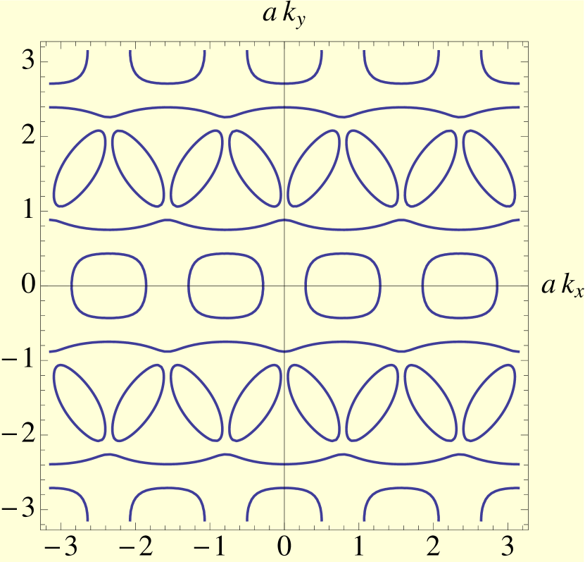
Figure 1: Reconstructed Fermi surafces with ${\bf Q}=\frac{\pi}{a}(\frac{3}{4},1)$, $W_{0}=0.65t$ , $V_{c}=0.05t$, and $\mu=-0.83t$. There are electron pockets, hole pockets and open orbits. The electron pocket frequency corresponds to $530\text{T}$ and the hole pockets to $280\text{T}$. The doping corresponds to $12.46\%$. Note that the figure is shown in the extended BZ for clarity.

To picture the current modulation and to define the order parameter of period-8 DDW in the real space Hamiltonian we need to calculate $\langle c_{{\bf R}^{\prime}}^{\dagger}c_{\bf R}\rangle$ for ${\bf R}^{\prime}\neq{\bf R}$. We get, correcting here a mistake in Ref. Dimov et al., 2008,

$$\begin{split}\langle c_{{\bf R}^{\prime}}^{\dagger}c_{\bf R}\rangle&=\frac{1}{N}\sum_{{\bf k}^{\prime}{\bf k}}\langle c_{{\bf k}^{\prime}}^{\dagger}c_{{\bf k}}\rangle\exp\left[-i({\bf k}^{\prime}\cdot{\bf R}^{\prime}-{\bf k}\cdot{\bf R})\right]\\ &=\pm\frac{iW_{0}}{2}(-1)^{n^{\prime}+m^{\prime}}\widetilde{V}_{{\bf R}^{\prime},{\bf R}},\end{split}$$ (4)

where ${\bf R}^{\prime}=(m^{\prime}a,n^{\prime}a)$, and $\widetilde{V}_{{\bf R}^{\prime},{\bf R}}$ is

$$\begin{split}\widetilde{V}_{{\bf R}^{\prime},{\bf R}}=&\Bigg{[}\frac{1+\cos 2\pi\eta}{2}(\delta_{{\bf R}^{\prime},{\bf R}+a{\bf\hat{x}}}+\delta_{{\bf R}^{\prime},{\bf R}-a{\bf\hat{x}}})\\ &-(\delta_{{\bf R}^{\prime},{\bf R}+a{\bf\hat{y}}}+\delta_{{\bf R}^{\prime},{\bf R}-a{\bf\hat{y}}})\Bigg{]}\cos 2m^{\prime}\pi\eta\\ &+\frac{\sin 2\pi\eta\sin 2m^{\prime}\pi\eta}{2}(\delta_{{\bf R}^{\prime},{\bf R}+a{\bf\hat{x}}}-\delta_{{\bf R}^{\prime},{\bf R}-a{\bf\hat{x}}}).\\ \end{split}$$ (5)

The current pattern is then

$$\begin{split}J_{{\bf R}^{\prime},{\bf R}}&=i[\langle c_{{\bf R}^{\prime}}^{\dagger}c_{\bf R}\rangle-\langle c_{\bf R}^{\dagger}c_{{\bf R}^{\prime}}\rangle]\\ &=-W_{0}(-1)^{n^{\prime}+m^{\prime}}\widetilde{V}_{{\bf R}^{\prime},{\bf R}},\end{split}$$ (6)

which is drawn in Fig. 2. The incommensurate $d$-density wave order parameter is proportional to

$$\widetilde{W}_{\mathbf{R^{\prime}},\mathbf{R}}=\frac{\mathrm{i}W_{0}}{2}(-1)^{n^{\prime}+m^{\prime}}\widetilde{V}_{\mathbf{R^{\prime}},\mathbf{R}}.$$ (7)

II.3 The real space Hamiltonian including disorder

In real space, the Hamiltonian in the presence of both disorder and magnetic field is

$$\begin{split}H=&\sum_{\mathbf{R}}\left[V(\mathbf{R})+2V_{c}\cos(\pi m/2)\right]c_{\mathbf{R}}^{\dagger}c_{\mathbf{R}}\\ &+\sum_{\mathbf{R^{\prime}},\mathbf{R}}t_{\mathbf{R^{\prime}},\mathbf{R}}~{}\mathrm{e}^{\mathrm{i}a_{\mathbf{R^{\prime}},\mathbf{R}}}c^{\dagger}_{\mathbf{R^{\prime}}}c_{\mathbf{R}}\\ &+\sum_{\mathbf{R^{\prime}},\mathbf{R}}\widetilde{W}_{\mathbf{R^{\prime}},\mathbf{R}}~{}\mathrm{e}^{\mathrm{i}a_{\mathbf{R^{\prime}},\mathbf{R}}}c^{\dagger}_{\mathbf{R^{\prime}}}c_{\mathbf{R}}+h.c.\end{split}$$ (8)

Here $t_{\mathbf{R^{\prime}},\mathbf{R}}$ defines the band structure: the nearest neighbor, the next nearest neighbor, and the third nearest neighbor hopping terms: $t$, $t^{\prime}$, $t^{\prime\prime}$. And $2V_{c}\cos(\frac{\pi}{2}m)$ is responsible for the period-four charge stripe order, where $m$ is $\mathbf{R}\cdot\hat{x}/a$ and $a$ is lattice spacing. We include correlated disorder in the form Jia et al. (2009)

$$V(\mathbf{R})=\frac{g_{V}}{2\pi l^{2}_{D}}\int~{}d\mathbf{x}~{}e^{-\frac{|\mathbf{R}-\mathbf{x}|^{2}}{2l^{2}_{D}}}~{}u(\mathbf{x}),$$ (9)

where $l_{D}$ is the disorder correlation length and the disorder averages are $\langle u(\mathbf{x})\rangle=0$ and $\langle u(\mathbf{x})u(\mathbf{y})\rangle=\delta(\mathbf{x}-\mathbf{y})$; the disorder intensity is set by $g_{V}$.

While white noise disorder seems to be more appropriate for NCCO with intrinsic disorder, correlated disorder may be more relevant to relatively clean YBCO samples in the range of well ordered chain compositions. Thus, here we shall focus on correlated disorder. A constant perpendicular magnetic field $B$ is included via the Peierls phase factor $a_{\mathbf{R^{\prime}},\mathbf{R}}=\frac{e}{\hbar c}\int_{\mathbf{R}}^{\mathbf{R^{\prime}}}\mathbf{A}\cdot\mathrm{d}\mathbf{l}$, where $\mathbf{A}=(0,-Bx,0)$ is the vector potential in the Landau gauge; the lattice vector ${\bf R}^{\prime}=(m^{\prime}a,n^{\prime}a)$ is defined by an arbitrary set of integers.

Figure 2: Current pattern for ${\bf Q}=(\frac{3\pi}{4a},\frac{\pi}{a})$. The relative magnitudes of the currents are depicted by the arrows in the legend. Note the antiphase domain wall structure.

III The transfer matrix method

The transfer matrix technique is a powerful method to compute conductance oscillations. It requires neither quasiclassical approximation nor ad hoc broadening of the Landau level to incorporate the effect of disorder. Various models of disorder, both long and short-ranged, can be studied ab initio. The mean field Hamiltonian, being a quadratic non-interacting Hamiltonian, leads to a Schrödinger equation for the site amplitudes, which is then recast in the form of a transfer matrix; the derivation has been discussed in detail previously. Jia et al. (2009); Eun et al. (2010) The conductance is then calculated by a formula that is well known in the area of mesoscopic physics, the Pichard-Landauer formula. Pichard and André (1986); *Fisher:1981 This yields Shubnikov-de Haas oscillations of the $ab$-plane resistivity, $\rho_{ab}$.

We consider a quasi-1D system, $N\gg M$, with a periodic boundary condition along y-direction. Here $Na$ is the length in the $x$-direction and $Ma$ is the length in the $y$-direction. Let $\Psi_{n}=(\psi_{n,1},\psi_{n,2},\ldots,\psi_{n,M})^{T}$, $n=1,\dots N$, be the amplitudes on the slice $n$ for an eigenstate with a given energy. Then the amplitudes between the successive slices depending on the Hamiltonian must form a given transfer matrix, $\mathbb{T}$.

The complete set of Lyapunov exponents, $\gamma_{i}$, of $\lim_{N\to\infty}({\cal T}_{N}{\cal T}_{N}^{\dagger})$, where ${\cal T}_{N}=\prod_{j=1}^{j=N}{\mathbb{T}}_{j}$ determine the conductance, $\sigma_{ab}(B)$ from the Pichard-Landauer formula:

$$\sigma_{ab}(B)=\frac{e^{2}}{h}\text{Tr}\sum_{j=1}^{2M}\frac{2}{({\cal T}_{N}{\cal T}_{N}^{\dagger})+({\cal T}_{N}{\cal T}_{N}^{\dagger})^{-1}+2}.$$ (10)

In this work we have chosen $M=30$ and $N$ of the order of $10^{5}$. This guaranteed $4\%$ accuracy of the smallest Lyapunov exponent. Note that at each step we have to invert a $4M\times 4M$ matrix and numerical errors prohibit much larger values of $M$.

IV Results

IV.1 Specific heat without disorder

The coefficient of the linear specific heat is

$$\gamma=\frac{\pi^{2}}{3}k_{B}^{2}\;\rho(0).$$ (11)

The density of states $\rho(\omega)$ measured with respect to the Fermi energy can be easily computed by taking into account all eight bands in the irreducible part of the Full Brillouin zone and a factor of 2 for spin. A Lorentzian broadening of the $\delta$-functions was used in computing the density of states. Although this is useful for numerical computation, the smoothing is a rough way of incorporating the effect of disorder on the density of states.

For a single CuO-layer we get,

$$\gamma\approx 5.4\frac{mJ}{mole.K^{2}},$$ (12)

where we have used the density of states at the Fermi energy from numerical calculation to be approximately 2.3 states/eV, as shown in the Figure 3. Including both layers $\gamma=2\times 5.4=10.8\frac{mJ}{mole.K^{2}}$, approximately a factor of 2 larger than the observed $5\frac{mJ}{mole.K^{2}}$ at $45T$. Riggs et al. (2011)

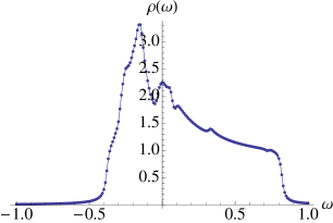
Figure 3: Total density of states, $t=0.15$, including eight bands in the reduced Brillouin zone per layer. The horizontal axis is in terms of electron volts and the vertical axis is a pure number, that is, the number of states. The rounding at the tails is due to the Lorentzian broadening of the $\delta$-functions by $\Gamma=0.1t$. The remaining parameters are the same as in Fig. 1. Further smoothing will reduce the density of states at the Fermi energy and lower the value of $\gamma$.

IV.2 Charge modulation without disorder

Before we carry out an explicit calculation it is useful to make a qualitative estimate. For $V_{c}=0.05t$, the total charge gap is to $4V_{c}=0.2t$. In order to convert to modulation of the charge order parameter, we have to divide by a suitable coupling constant. In high temperature superconductors, all important coupling constants are of the order bandwidth, which is $8t=1.2eV$. Taking this as a rough estimate, we deduce that the charge modulation is $0.025e$, expressed in terms of electronic charge.

To explicitly calculate charge modulation at a site, we diagonalize the $8\times 8$ Hamiltonian matrix $Z(k_{x},k_{y})$ for each k in the reduced Brillouin zone (RBZ). We get 8 eigenvalues and the corresponding eigenvectors: $E_{n,k_{x},k_{y}}$ and $\psi_{n,k_{x},k_{y}}$ for $n=1,2,...,8$. The eigenvector $\psi_{n,k_{x},k_{y}}$ has eight components of the form:

$$\psi_{n,k_{x},k_{y}}=(\alpha_{n,k_{x},k_{y}}(1),\alpha_{n,k_{x},k_{y}}(2),....,\alpha_{n,k_{x},k_{y}}(8))$$ (13)

Then the wave function in the real space for each state $\{n,k_{x},k_{y}\}$ is

$$\psi_{n,k_{x},k_{y}}(\mathbf{R})=\sum_{j=1}^{8}\alpha_{n,k_{x},k_{y}}(j)\frac{1}{\sqrt{N}}\exp{i(\mathbf{k}+(j-1)\mathbf{Q})\cdot\mathbf{R}}$$ (14)

So, by definition, the local number density is

$$n(\mathbf{R})=2\times{\sum_{n,k_{x},k_{y}}}^{\prime}\left|{\psi_{n,k_{x},k_{y}}(\mathbf{R})}\right|^{2}$$ (15)

Here the prime in the sum means that all occupied states with energy below the chemical potential are considered. The factor of 2 is for spin and the summation over $k_{x},k_{y}$ is performed in the RBZ. For different parameter sets the numerical results are:

• Parameter set 1
  $W_{0}=0.71t,V_{c}=0.05t,\mu=-0.78t,x=11.73\%$
  Averaged number density of electron is $n=0.894$ per site, while the estimated deviation is about $\delta n=0.059$ per site. So $\delta n/n=6.6\%$.

• Parameter set 2
  $W_{0}=0.65t,V_{c}=0.05t,\mu=-0.83t,x=12.46\%$
  Averaged number density of electron is: $n=0.893$ per site, while the estimated deviation is about $\delta n=0.062$ per site. So $\delta n/n=6.9\%$.

Of course, for both cases, the period of the CDW modulation is $4a$, where $a$ is the lattice spacing. It is also interesting to calculate the ratio of the modulation of the local density of states to the average density of states at the Fermi energy; we find $\delta\rho(\mu)/\rho(\mu)\approx 13-15\%$ depending on the parameters. As pointed out in Ref. Yao et al., 2011, this leads to an estimate of the corresponding variation of the Knight shift.

IV.3 Oscillation spectra in the presence of correlated disorder

Previously it was found from the consideration of $1/8$ magnetic antiphase stripe order that there is a remarkable variety of possible Fermi surface reconstructions depending on the choice of parameters. Millis and Norman (2007) This is also true for the incommensurate period-8 DDW. In contrast, two-fold commensurate DDW order leads to much lesser variety. While this is more satisfying, period-4 charge modulation observed in NMR measurements Wu et al. (2011) and the non-existence of the larger hole pocket commensurate with the Luttinger sum rule have forced us to take seriously the period-8 DDW. This requires a judicious choice of parameters of the model.

Although we cannot constrain the parameters uniquely, we have used a number of guiding principles. First, disorder was chosen to be correlated with a length scale $\ell_{D}$ smaller than the transverse width of the strip, $Ma$. Since the YBCO samples studied appear to have lesser degree of disorder than the intrinsic disorder of NCCO, the white noise disorder did not appear sensible. Because the experimentally measured charge modulation in NMR is $0.03\pm 0.01e$, it is necessary to keep $V_{c}$ small enough to be consistent with experiments. A value of $V_{c}$ in the neighborhood of $0.05t$ seemed reasonable. Of course, this could be adjusted to agree precisely with experiments, but this would not have been very meaningful.

The band structure parameter $t$ was chosen to be $0.15eV$ as opposed to LDA value of $0.38eV$. Although reliable ARPES measurements are not available for YBCO, measurements in other cuprates have indicated that the bandwidth is renormalized by at least a factor of 2. Had we chosen $t=0.38eV$, the agreement with specific heat measurements would have been essentially perfect, but we could not see any justification for this. The parameters $t^{\prime}/t$ and $t^{\prime\prime}/t^{\prime}$ are same as the commonly used LDA values, as the shape of the Fermi surface in most cases appear to be given correctly by LDA. We searched the remaining parameters, $\mu$, $g_{V}$ and $W_{0}$, extensively. There are a number of issues worth noting. Oscillation spectra hardly ever show any substantial evidence of harmonics, which should be used as a constraining factor. Moreover, as we believe that it is the electron pocket that is dominant in producing negative $R_{H}$, it is necessary that we do not employ parameters that wipe out the electron pocket altogether. The coexistence of electron and hole pockets give a simple explanation of the oscillations of $R_{H}$ as a function of the magnetic field. We generically found hole pocket frequencies in the range $150-300\text{T}$. This is one of our crucial observations. It implies that to resolve clearly such a slow frequency, one must go to much higher fields than are currently possible. We argue that this may be a plausible reason why the hole pocket has not been observed except for one experiment which goes up to $85\text{T}$; in this experiment some evidence of a $250\text{T}$ frequency is observed. Singleton et al. (2010)

A further constraining fact is that no evidence of magnetic breakdown is observed in YBCO, while in NCCO it is clearly present. This implies that our parameters should be consistent with this fact. The DDW gap and the disorder level are consistent with the observed data. Overall we find satisfactory consistency with doping levels between $11-12.5\%$ within our calculational scheme. Lower doping levels produce less satisfactory agreement, but can be made better with further adjustment of parameters, but we have avoided fine tuning as much as possible. The broad brush picture can already be seen in the oscillation spectra in Figs.  4,  5,  6, and  7. Two general trends are that electron pockets dominate at higher doping levels within the range we have checked, and an increase in disorder intensity reduces the intensity of the Fourier spectra of the electron pockets. A few harmonics are still present.

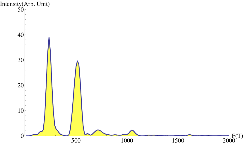
Figure 4: Fourier transform of the oscillation spectra after a background subtraction with a cubic polynomial. $W_{0}=0.71t$, $V_{c}=0.05t$, $\mu=-0.78t$, $M=30\;a$, $N=10^{5}\;a$, $\ell_{D}=8\;a$, $g_{V}=0.1t$. Doping is $11.73\%$.

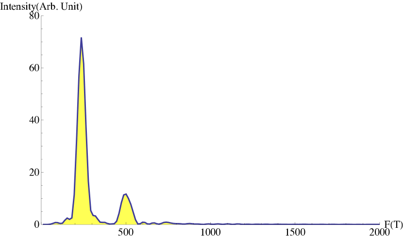
Figure 5: Fourier transform of the oscillation spectra after a background subtraction with a cubic polynomial. $W_{0}=0.71t$, $V_{c}=0.05t$, $\mu=-0.78t$, $M=30\;a$, $N=10^{5}\;a$, $\ell_{D}=8\;a$, $g_{V}=0.3t$. Doping is $11.73\%$.

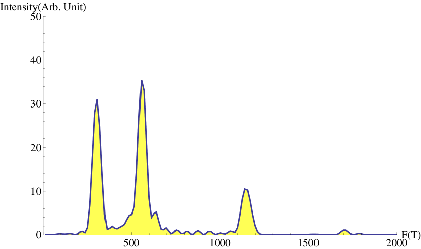
Figure 6: Fourier transform of the oscillation spectra after a background subtraction with a cubic polynomial. $W_{0}=0.65t$, $V_{c}=0.05t$, $\mu=-0.83t$, $M=30\;a$, $N=10^{5}\;a$, $\ell_{D}=8\;a$, $g_{V}=0.1t$. Doping is $12.46\%$.

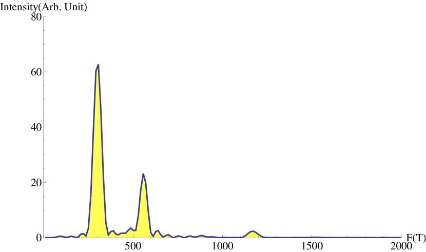
Figure 7: Fourier transform of the oscillation spectra after a background subtraction with a cubic polynomial. $W_{0}=0.65t$, $V_{c}=0.05t$, $\mu=-0.83t$, $M=30\;a$, $N=10^{5}\;a$, $\ell_{D}=8\;a$, $g_{V}=0.2t$. Doping is $12.46\%$.

V Discussion and outlook

The complex materials physics of high temperature superconductors lead to a fairly large number of dimensionless parameters. Thus, it is not possible to frame a unique theory. Tuning these parameters can indeed lead to many different phases. However, there may be a general framework that could determine the overall picture. To be more specific, let us consider the quantum oscillation measurements that we have been discussing here.

• Are the applied magnetic fields sufficiently large to essentially destroy all traces of superconductivity and thereby reveal the underlying normal state from which superconductivity develops? While for NCCO this is clearcut because $H_{c2}$ is less than $10\text{T}$, while the quantum oscillation measurements are carried out between $30-65\text{T}$, far above $H_{c2}$. For YBCO lingering doubts remain. However, one may argue that the high field measurements are such that one may be in a vortex liquid state where the slower vortex degrees of freedom may simply act as quenched disorder to the nimble electrons. This is the picture we have adopted here.

• The emergent picture of Fermi pockets are seemingly at odds with ARPES, unless only half the pocket is visible in ARPES, as was previously argued. Chakravarty et al. (2003) On the other hand, reliable ARPES in YBCO is not available. For electron doped NCCO or PCCO this appears not be true. Armitage et al. (2009)

• Almost all scenarios place the observed electron pockets at the anti-nodal points in the Brillouin zone, while many other experiments would require the pseudogap to be maximum there. One may, however, question if there is only one pseudo gap.

• Quantum oscillations of $R_{H}$ are easier to explain if there are at least two closed pockets in the Boltzmann picture. Chakravarty and Kee (2008) Thus associated with the electron pocket there must be a hole pocket or vice versa. This is not a problem with NCCO, as we have shown how magnetic breakdown, Eun et al. (2010) and a greater degree of intrinsic disorder, provides a simple resolution as to why only one pocket, in this case a small but prominent hole pocket is seen. In any case, oscillations of $R_{H}$ in NCCO is yet to be measured. With respect to YBCO this becomes a serious problem. Any commensurate picture would lead to a hole pocket of frequency about twice that of the electron pocket frequency if the Luttinger sum rule is to be satisfied. Despite motivated effort no evidence in this regard has emerged. An escape from the dilemma is to propose an incommensurate picture in which the relevant electron pocket is accompanied by a much smaller hole pocket and some open orbits, as we have done here. In order to convincingly observe such small hole pocket, one would require extending these measurements to almost impossibly higher fields; see, however, Ref. Singleton et al., 2010.

• All oscillation measurements to date have been convincingly interpreted in terms of the Lifshitz-Kosevich theory for which the validity of Fermi liquid theory and the associated Landau levels seem to be obligatory. Why should the normal state of an under doped cuprate behave like a Fermi liquid?

• The contrast between electron and hole doped cuprates is interesting. In NCCO the crystal structure consists of a single CuO plane per unit cell, and, in contrast to YBCO, there are no complicating chains, bilayers, ortho-II potential, stripes, etc. Armitage et al. (2009) Thus, it would appear to be ideal for gleaning the mechanism of quantum oscillations. On the other hand, disorder in NCCO is significant. It is believed that well-ordered chain materials of YBCO contain much less disorder by comparison.

• In YBCO, studies involving tilted field seem to rule out triplet order parameter, hence SDW. Ramshaw et al. (2011); Sebastian et al. (2011) Moreover, from NMR measurements at high fields, there appears to be no evidence of a static spin density wave order in YBCO. Wu et al. (2011) Similarly there is no evidence of SDW order in fields as high as $23.2T$ in $\mathrm{YBa_{2}Cu_{4}O_{8}}$ Zheng et al. (1999), while quantum oscillations are clearly observed in this material. Yelland et al. (2008); Bangura et al. (2008) Also no such evidence of SDW is found up to $44T$ in $\mathrm{Bi_{2}Sr_{2-x}La_{x}CuO_{6+\delta}}$. Kawasaki et al. (2011) At present, results from high field NMR in NCCO does not exist, but measurements are in progress. Brown (2011) The zero field neutron scattering measurements indicate very small spin-spin correlation length in the relevant doping regime. Motoyama et al. (2007) Energetically a perturbation even as large as $45T$ field is weak. Nguyen and Chakravarty (2002)

• As to singlet order, relevant to quantum oscillations, Garcia-Aldea and Chakravarty (2011); *Norman:2011; *Ramazashvili:2011 charge density wave is a possibility, which has recently found some support in the high field NMR measurements in YBCO. Wu et al. (2011) But since the mechanism is helped by the oxygen chains, it is unlikely that the corresponding NMR measurements in NCCO will find such a charge order. Moreover, the observed charge order in YBCO sets in at a much lower temperature ($20-50K$) compared to the pseudogap. Thus the charge order may be parasitic. As to singlet DDW, there are two neutron scattering measurements that seem to provide evidence for it. Mook et al. (2002); *Mook:2004 However, these measurements have not been confirmed by further independent experiments. However, DDW order should be considerably hidden in NMR involving nuclei at high symmetry points, because the orbital currents should cancel.

As mentioned above, a mysterious feature of quantum oscillations in YBCO is the fact that only one type of Fermi pockets is observed. If two-fold commensurate density wave is the mechanism, this will violate the Luttinger sum rule. Luttinger (1960); *Chubukov:1997; *Altshuler:1998; Chakravarty and Kee (2008) We had previously provided an explanation of this phenomenon in terms of disorder arising from both defects and vortex scattering in the vortex liquid phase; Jia et al. (2009) however, the arguments are not unassailable. In contrast, for NCCO, the experimental results are quite consistent with a simple theory presented previously. The present work, based on incommensurate DDW, may provide another, if not a more plausible alternative in YBCO.

The basic question as to why Fermi liquid concepts should apply remains an important unsolved mystery. Chakravarty (2011) It is possible that if the state revealed by applying a high magnetic field has a broken symmetry with an order parameter (hence a gap), the low energy excitations will be quasiparticle-like, not a spectra with a branch cut, as in variously proposed strange metal phases.

VI Acknowledgments

We would like to thank S. Kivelson and B. Ramshaw for very helpful discussion. This work is supported by NSF under the Grant DMR-1004520.

References

- Doiron-Leyraud et al. (2007) N. Doiron-Leyraud, C. Proust, D. LeBoeuf, J. Levallois, J.-B. Bonnemaison, R. Liang, D. A. Bonn, W. N. Hardy, and L. Taillefer, Nature 447, 565 (2007).
- Chakravarty (2008) S. Chakravarty, Science 319, 735 (2008).
- Yelland et al. (2008) E. A. Yelland, J. Singleton, C. H. Mielke, N. Harrison, F. F. Balakirev, B. Dabrowski, and J. R. Cooper, Phys. Rev. Lett. 100, 047003 (2008).
- Bangura et al. (2008) A. F. Bangura, J. D. Fletcher, A. Carrington, J. Levallois, M. Nardone, B. Vignolle, P. J. Heard, N. Doiron-Leyraud, D. LeBoeuf, L. Taillefer, S. Adachi, C. Proust, and N. E. Hussey, Phys. Rev. Lett. 100, 047004 (2008).
- Millis and Norman (2007) A. J. Millis and M. R. Norman, Phys. Rev. B 76, 220503 (2007).
- Chakravarty and Kee (2008) S. Chakravarty and H.-Y. Kee, Proc. Natl. Acad. Sci. USA 105, 8835 (2008).
- Dimov et al. (2008) I. Dimov, P. Goswami, X. Jia, and S. Chakravarty, Phys. Rev. B 78, 134529 (2008).
- Podolsky and Kee (2008) D. Podolsky and H.-Y. Kee, Physical Review B 78, 224516 (2008).
- Chen and Lee (2009) K.-T. Chen and P. A. Lee, Phys. Rev. B 79, 180510 (2009).
- Yao et al. (2011) H. Yao, D.-H. Lee, and S. Kivelson, Phys. Rev. B 84, 012507 (2011).
- Helm et al. (2009) T. Helm, M. V. Kartsovnik, M. Bartkowiak, N. Bittner, M. Lambacher, A. Erb, J. Wosnitza, and R. Gross, Phys. Rev. Lett. 103, 157002 (2009).
- Helm et al. (2010) T. Helm, M. V. Kartsovnik, I. Sheikin, M. Bartkowiak, F. Wolff-Fabris, N. Bittner, W. Biberacher, M. Lambacher, A. Erb, J. Wosnitza, and R. Gross, Phys. Rev. Lett. 105, 247002 (2010).
- Kartsovnik and et al. (2011) M. V. Kartsovnik and et al., New J. Phys. 13, 015001 (2011).
- Eun et al. (2010) J. Eun, X. Jia, and S. Chakravarty, Phys. Rev. B 82, 094515 (2010).
- Eun and Chakravarty (2011) J. Eun and S. Chakravarty, Phys. Rev. B 84, 094506 (2011).
- Taillefer (2009) L. Taillefer, Journal of Physics: Condensed Matter 21, 164212 (2009).
- Ramshaw et al. (2011) B. J. Ramshaw, B. Vignolle, R. Liang, W. N. Hardy, C. Proust, and D. A. Bonn, Nat. Phys. 7, 234 (2011).
- Sebastian et al. (2011) S. E. Sebastian, N. Harrison, M. M. Altarawneh, F. F. Balakirev, C. H. Mielke, R. Liang, D. A. Bonn, W. N. Hardy, and G. G. Lonzarich, “Direct observation of multiple spin zeroes in the underdoped high temperature superconductor ,” (2011), arXiv:1103.4178v1 [cond-mat] .
- Wu et al. (2011) T. Wu, H. Mayaffre, S. Kramer, M. Horvatic, C. Berthier, W. Hardy, R. Liang, D. Bonn, and M.-H. Julien, Nature 477, 191 (2011).
- Lederer and Kivelson (2011) S. Lederer and S. Kivelson, “Observable NMR signal from circulating current order in YBCO,” (2011), arXiv:1112.1755 .
- Nayak (2000) C. Nayak, Phys. Rev. B 62, 4880 (2000).
- Chakravarty et al. (2001) S. Chakravarty, R. B. Laughlin, D. K. Morr, and C. Nayak, Phys. Rev. B 63, 094503 (2001).
- Singleton et al. (2010) J. Singleton, C. de la Cruz, R. D. McDonald, S. Li, M. Altarawneh, P. Goddard, I. Franke, D. Rickel, C. H. Mielke, X. Yao, and P. Dai, Phys. Rev. Lett. 104, 086403 (2010).
- Hossain et al. (2008) M. A. Hossain, J. D. F. Mottershead, D. Fournier, A. Bostwick, J. L. McChesney, E. Rotenberg, R. Liang, W. N. Hardy, G. A. Sawatzky, I. S. Elfimov, D. A. Bonn, and A. Damascelli, Nat Phys 4, 527 (2008).
- Damascelli et al. (2003) A. Damascelli, Z. Hussain, and Z. X. Shen, Rev. Mod. Phys. 75, 473 (2003).
- Pavarini et al. (2001) E. Pavarini, I. Dasgupta, T. Saha-Dasgupta, O. Jepsen, and O. K. Andersen, Phys. Rev. Lett. 87, 047003 (2001).
- Sassa et al. (2011) Y. Sassa, M. Radović, M. Månsson, E. Razzoli, X. Y. Cui, S. Pailhès, S. Guerrero, M. Shi, P. R. Willmott, F. Miletto Granozio, J. Mesot, M. R. Norman, and L. Patthey, Phys. Rev. B 83, 140511 (2011).
- Jia et al. (2009) X. Jia, P. Goswami, and S. Chakravarty, Phys. Rev. B 80, 134503 (2009).
- Pichard and André (1986) J. L. Pichard and G. André, Europhys. Lett. 2, 477 (1986).
- Fisher and Lee (1981) D. S. Fisher and P. A. Lee, Phys. Rev. B 23, 6851 (1981).
- Riggs et al. (2011) S. C. Riggs, O. Vafek, J. B. Kemper, J. Betts, A. Migliori, W. N. Hardy, R. Liang, D. A. Bonn, and G. Boebinger, Nat. Phys. 7, 332 (2011).
- Chakravarty et al. (2003) S. Chakravarty, C. Nayak, and S. Tewari, Phys. Rev. B 68, 100504 (2003).
- Armitage et al. (2009) N. P. Armitage, P. Fournier, and R. L. Green, Rev. Mod. Phys. 82, 2421 (2009).
- Zheng et al. (1999) G.-q. Zheng, W. G. Clark, Y. Kitaoka, K. Asayama, Y. Kodama, P. Kuhns, and W. G. Moulton, Phys. Rev. B 60, R9947 (1999).
- Kawasaki et al. (2011) S. Kawasaki, C. Lin, P. L. Kuhns, A. P. Reyes, and G.-q. Zheng, Phys. Rev. Lett. 105, 137002 (2011).
- Brown (2011) S. E. Brown, (2011).
- Motoyama et al. (2007) E. M. Motoyama, G. Yu, I. M. Vishik, O. P. Vajk, P. K. Mang, and M. Greven, Nature 445, 186 (2007).
- Nguyen and Chakravarty (2002) H. K. Nguyen and S. Chakravarty, Phys. Rev. B 65, 180519 (2002).
- Garcia-Aldea and Chakravarty (2011) D. Garcia-Aldea and S. Chakravarty, Phys. Rev. B 82, 184526 (2011).
- Norman and Lin (2011) M. R. Norman and J. Lin, Phys. Rev. B 82, 060509 (2011).
- Ramazashvili (2011) R. Ramazashvili, Phys. Rev. Lett. 105, 216404 (2011).
- Mook et al. (2002) H. A. Mook, P. Dai, S. M. Hayden, A. Hiess, J. W. Lynn, S. H. Lee, and F. Doǧan, Phys. Rev. B 66, 144513 (2002).
- Mook et al. (2004) H. A. Mook, P. Dai, S. M. Hayden, A. Hiess, S. H. Lee, and F. Doǧan, Phys. Rev. B 69, 134509 (2004).
- Luttinger (1960) J. M. Luttinger, Phys. Rev. 119, 1153 (1960).
- Chubukov and Morr (1997) A. V. Chubukov and D. K. Morr, Phys. Rep. 288, 355 (1997).
- Altshuler et al. (1998) B. L. Altshuler, A. V. Chubukov, A. Dashevskii, A. M. Finkel’stein, and D. K. Morr, Europhys. Lett. 41, 401 (1998).
- Chakravarty (2011) S. Chakravarty, Rep. Prog. Phys. 74, 022501 (2011).