Steady base states for non-Newtonian granular hydrodynamics

Abstract

We study in this work steady laminar flows in a low density granular gas modelled as a system of identical smooth hard spheres that collide inelastically. The system is excited by shear and temperature sources at the boundaries, which consist of two infinite parallel walls. Thus, the geometry of the system is the same that yields the planar Fourier and Couette flows in standard gases. We show that it is possible to describe the steady granular flows in this system, even at large inelasticities, by means of a (non-Newtonian) hydrodynamic approach. All five types of Couette–Fourier granular flows are systematically described, identifying the different types of hydrodynamic profiles. Excellent agreement is found between our classification of flows and simulation results. Also, we obtain the corresponding non-linear transport coefficients by following three independent and complementary methods: (1) an analytical solution obtained from Grad’s 13-moment method applied to the inelastic Boltzmann equation, (2) a numerical solution of the inelastic Boltzmann equation obtained by means of the direct simulation Monte Carlo method and (3) event-driven molecular dynamics simulations. We find that, while Grad’s theory does not describe quantitatively well all transport coefficients, the three procedures yield the same general classification of planar Couette–Fourier flows for the granular gas.

1 Introduction

There have been in the recent years a large number of studies on the dynamics of granular gases, where ‘granular gas’ is a term used to refer to a low density system of many mesoscopic particles that collide inelastically in pairs. Due to inelasticity in the collisions, the granular gas particles tend to collapse to a rest state, unless there is some kind of energy input. In particular, Goldhirsch & Zanetti (1993) showed that clustering instabilities spontaneously appear in a freely evolving granular gas. Nevertheless, most situations of practical interest involve an energy input to compensate for the energy loss and sustain, in some cases, the ‘gas’ condition of the granular system. This type of problem has been extensively studied, giving rise to a subfield of granular dynamics: ‘rapid granular flows’ (Jenkins & Savage, 1983; Wang, Jackson & Sundaresan, 1996; Goldhirsch, 2003; Aranson & Tsimring, 2006). Furthermore, it has been shown that rapid granular flows can attain steady states, some of which, under appropriate circumstances and for simple geometries, can give rise to laminar flows, in the same way as a regular gas does (see, for instance, the work by Tij, Tahiri, Montanero, Garzó, Santos & Dufty, 2001, on Couette granular flows). The question arising (Goldhirsch, 2003) is, what is the appropriate theoretical approach to study these granular flows?

Let us start with classical non-equilibrium statistical mechanics for an ideal gas described by the Boltzmann equation (Chapman & Cowling, 1970). As is well known, the equilibrium velocity distribution function $f(\boldsymbol{r},\boldsymbol{v},t)$ for an ordinary (i.e., elastic) gas is the Maxwell–Boltzmann distribution (Huang, 1987). For non-equilibrium states, however, the solution of the Boltzmann equation is generally not known. On the other hand, in some cases, there exist special solutions where all the space and time dependence of $f(\boldsymbol{r},\boldsymbol{v},t)$ occurs only through a functional dependence on the average fields $n$ (density), $\boldsymbol{u}$ (flow velocity) and $T$ (temperature) associated with the conserved quantities (mass, momentum and energy) (Chapman & Cowling, 1970). This type of solution is called a normal solution of the Boltzmann equation (Cercignani, 1988). As a consequence, the momentum and heat fluxes are also functionals of the hydrodynamic fields and thus the balance equations become a closed set of equations for those fields. Therefore, the normal solutions of the Boltzmann equation yield a hydrodynamic description (Haff, 1983), since the closed set of equations is actually formally similar to the traditional fluid mechanics equations (Chapman & Cowling, 1970). In practice, what we have got is a transition from a microscopic description (based on the distribution function) to a macroscopic description (based on the average fields) (Hilbert, 1912).

When the strength of the hydrodynamic gradients is small, the above functional dependence of the non-uniform distribution function $f$ on $n,\boldsymbol{u},T$ can be constructed by means of the Chapman–Enskog method (Chapman & Cowling, 1970), whereby $f$ is expressed as a series in a formal parameter $\epsilon$:

$$f=f^{(0)}+f^{(1)}\epsilon+f^{(2)}\epsilon^{2}+f^{(3)}\epsilon^{3}+\cdots.$$ (1)

The parameter $\epsilon$ indicates the order in the spatial gradients of the average fields, scaled with the inverse of a typical microscopic length unit (mean free path, for instance). If terms up to only first order in the gradients are considered ($f\simeq f^{(0)}+f^{(1)}\epsilon$), the mass, momentum and energy balance equations are the well known Navier–Stokes (NS) equations of fluid mechanics (Chapman & Cowling, 1970; Cercignani, 1988). This approach is accurate for problems where the spatial gradients are sufficiently small. For not so small gradients, terms up to second order in the gradients need to be considered, and we obtain the Burnett equations (Burnett, 1935), used for instance in rarefied gases (Montanero, López de Haro, Garzó & Santos, 1998, 1999; Agarwal, Yun & Balakrishnan, 2001). For both NS and Burnett equations, the expressions for the fluxes include a set of parameters called ‘hydrodynamic transport coefficients’.

Regarding the granular gas, and from a theoretical point of view, it makes sense in principle, due to the system’s low density, to derive the dynamics from a closed kinetic equation for the distribution function of a single particle, in an analogous way to the standard gas (Goldhirsch, 2003); i.e., it is assumed that pre-collisional velocities are not statistically correlated (or, at least, that their correlations are not important). Thus, the corresponding kinetic equation is analogous to the Boltzmann equation but with the modification that inelasticity introduces in the collision integral part (Brey, Dufty, Kim & Santos, 1998; Goldhirsch, 2003). We may call this modified version of the Boltzmann equation ‘inelastic Boltzmann equation’ (Brey et al., 1998; Goldhirsch, 2003). In addition, if we assume the existence of a normal solution to the inelastic Boltzmann equation, a hydrodynamic description analogous to that described above for an elastic gas results for a granular gas; i.e., transport coefficients and a set of hydrodynamic equations may be derived. This is obviously a question of much interest in the description of transport properties of large sets of grains at low density.

However, due to the coupling between spatial gradients and inelasticity in steady states (Sela & Goldhirsch, 1998; Santos, Garzó & Dufty, 2004), the collisional cooling sets the strength of the spatial gradients and thus scale separation might not occur (i.e., gradients might not be small), except in the limit of quasi-elastic collisions (Vega Reyes & Urbach, 2009). Therefore, NS or Burnett hydrodynamics would only be expected to work well for steady granular flows in the quasi-elastic limit. Nevertheless, some recent works have found that a non-Newtonian hydrodynamic description of planar laminar flows, beyond Burnett order, is still possible for moderately large spatial gradients, even for large inelasticity (Tij, Tahiri, Montanero, Garzó, Santos & Dufty, 2001; Santos, Garzó & Vega Reyes, 2009; Vega Reyes, Santos & Garzó, 2010, 2011a). Actually, it is not surprising that a generalized hydrodynamic description of the Boltzmann inelastic equation works in rapid granular flows, even for moderately large gradients, since this is also possible when strong gradients occur in elastic gases (Agarwal et al., 2001; Garzó & Santos, 2003). We have pointed out previously that this implies that hydrodynamics for granular gases is a generalization of classic hydrodynamics for elastic gases. Furthermore, a special class of flows has been recently found in a unified hydrodynamic description valid for elastic and inelastic gases (Vega Reyes et al., 2010, 2011a). Thus, the only formal difference between transport theory for granular and ordinary gases would emerge not from the limitations due to scale separation but from the possible influence of statistical correlations arising from memory effects due to inelasticity. In fact, there is a number of works showing velocity correlations in systems of inelastic particles (for instance, see the work by McNamara & Luding, 1998; Soto & Mareschal, 2001; Soto, Piasecki & Mareschal, 2001; Pagonabarraga, Trizac, van Noije & Ernst, 2002; Prevost, Egolf & Urbach, 2002; Brilliantov, Pöschel, Kranz & Zippelius, 2007) and elastic particles (Schlamp & Hathorn, 2007). This statistical effect would have its origin at the more fundamental level of the kinetic equation (the inelastic Boltzmann equation). Put in other words, if the Boltzmann inelastic equation is to be valid, hydrodynamic solutions for steady granular flows arising from it should work, as has been previously shown by different authors (Alam & Nott, 1998; Tij et al., 2001; Vega Reyes et al., 2010). As a matter of fact, the inelastic Boltzmann equation has been used, with good results, as the starting point in an overwhelming number of studies on rapid granular flows (Goldhirsch, 2003; Aranson & Tsimring, 2006). Additionally, good agreement has also been shown, for a variety of rapid granular flows, between hydrodynamic theory (stemming from the inelastic Boltzmann equation) and molecular dynamics results (in which the velocity statistical correlations would be inherently present, see the works by Prevost, Egolf & Urbach, 2002; Lutsko, Brey & Dufty, 2002; Dahl, Hrenya, Garzó & Dufty, 2002; Alam & Luding, 2003; Montanero, Garzó, Alam & Luding, 2006). Furthermore, in the case of the special class mentioned before, the agreement of molecular dynamics results with (Grad’s) hydrodynamic theory is excellent (Vega Reyes et al., 2010, 2011a).

A considerable amount of work has been devoted to systematic calculations of hydrodynamic transport coefficients for granular gas systems, with different degrees of approach in the perturbative solution of the non-uniform distribution function (Sela & Goldhirsch, 1998; Brey et al., 1998; Goldhirsch, 2003; Nott et al., 1999; Alam et al., 2005). However, the derivation of non-Newtonian transport coefficients in simple laminar flows has been probably not as systematic as for the case of NS transport coefficients.

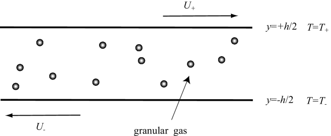
Figure 1: Schematic view of the system subject of study. The granular gas is heated and sheared from two infinite parallel walls. Walls are located at $y=\pm h/2$ and have temperatures $T_{\pm}$ and velocities $U_{\pm}$, respectively.

The main goal of this paper is the systematic derivation, by means of a non-Newtonian hydrodynamic approach, of the steady profiles for laminar granular flows in the simple geometry of two infinite parallel walls containing the gas. More specifically, shear and energy are input from the walls (see figure 1). In the theoretical approach we assume that (i) the hydrostatic pressure $p$ is constant, (ii) the reduced shear rate $a$ (i.e., the ratio between the local shear rate and the local collision frequency) is also constant, (iii) the shear stress is independent of the granular temperature gradient $\partial_{y}T$, whereas (iv) the heat flux $q_{y}$ is proportional to $\partial_{y}T$. As we will see, the resulting classification of profiles is formally analogous to the one found for NS hydrodynamics in the quasielastic limit (Vega Reyes & Urbach, 2009), except that the constitutive relations are non-linear. This classification is done based on the signs of $\partial_{y}(T^{1/2}\partial_{y}T)$ and $\partial_{y}^{2}T$. As we will show, both signs remain constant throughout the system and are related to the competition between viscous heating and inelastic cooling. Moreover, the sign of $\partial_{y}^{2}T$ is also governed by the wall temperature difference. In the case of elastic collisions, only the viscous heating effect is present and so $\partial_{y}(T^{1/2}\partial_{y}T)<0$, which implies $\partial_{y}^{2}T<0$ (Garzó & Santos, 2003). Therefore, the general classification is only relevant for granular gases and, consequently, the case of ordinary gases is embedded as a particular case.

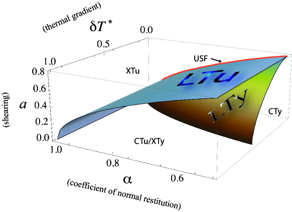
Figure 2: Each point of this diagram represents a steady-state Couette–Fourier flow defined univocally by the set of parameters $\delta T^{*}$ (difference between the temperatures at the top and bottom fluid layers, divided by the wall separation), $a$ (reduced shear rate) and $\alpha$ (coefficient of restitution), the two first ones being determined from the boundary conditions. The surface with the label LTu defines the class of states where the temperature $T$ is a linear function of the flow velocity $u_{x}$, while the surface labelled as LTy (below the LTu surface) defines the class with a linear profile $T(y)$. Both surfaces intersect in the line representing the uniform shear flow (USF), located in the $\delta T^{*}=0$ plane. In addition, the LTu surface contains the line corresponding to Fourier flows for ordinary gases (represented by the $\delta T^{*}$ axis, i.e., $a=0$ and $\alpha=1$). The point $\delta T^{*}=0$, $a=0$ and $\alpha=1$ (not visible in the diagram) represents the equilibrium state of an ordinary gas. Notice that, whereas the LTu surface has points for all values of $\delta T^{*}$, the LTy surface has an upper bound of $\delta T^{*}$ which occurs at $a=0$ for each $\alpha$. The LTu and LTy surfaces split the space into three regions: XTu, CTu/XTy and CTy (see § 5.3).

The hypotheses (i)–(iv) are sensible for a number of reasons. First, they have shown a good agreement with computer simulations in previous works on Couette granular gas flows in the particular case $\partial_{y}(T^{1/2}\partial_{y}T)<0$ (Tij et al., 2001). In addition, there exists a special class of flows, including both elastic and inelastic flows (Vega Reyes & Urbach, 2009; Santos et al., 2009; Vega Reyes et al., 2010, 2011a), characterized by $\partial_{y}(T^{1/2}\partial_{y}T)=0$. This special class defines a surface in the three-parameter space conformed by inelasticity (represented by the coefficient of normal restitution $\alpha$), reduced shear rate and thermal gradient, as shown in figure 2. It is called ‘LTu’ surface since this class of flows is characterized by having linear $T(u_{x})$ profiles (Vega Reyes et al., 2010, 2011a). The LTu surface splits the parameter space into two regions: the first region (above the LTu surface in figure 2 and labelled XTu) corresponds to $\partial_{y}(T^{1/2}\partial_{y}T)<0$ (i.e., viscous heating overcomes inelastic cooling), while the second region (below the LTu surface) has $\partial_{y}(T^{1/2}\partial_{y}T)>0$ (i.e., inelastic cooling dominates). As we will see, the region below the LTu surface can also be split into two sub-regions (labelled CTu/XTy and CTy), depending on the sign of $\partial_{y}^{2}T$, separated by a surface where $\partial_{y}^{2}T=0$. The latter surface is called here ‘LTy’ because it corresponds to states where $T(y)$ is a linear function. To the best of our knowledge, the regions below the LTu surface have not been explored before for $a\neq 0$, except in the NS description (Vega Reyes & Urbach, 2009). All other studies below the LTu surface have been restricted to the plane $a=0$ in figure 2 (see, for instance, the works by Grossman, Zhou & Ben-Naim, 1997; Brey & Cubero, 1998; Brey, Ruiz-Montero & Moreno, 2000). The most prominent result in studies for the $a=0$ plane is perhaps the finding of LTy states (Brey, Cubero, Moreno & Ruiz-Montero, 2001, 2009, 2011, 2012), which are represented in figure 2 by the intersection curve between the LTy surface and the plane $a=0$.

Our purpose is now to extend results obtained in previous works by providing a comprehensive description of granular/elastic Couette–Fourier gas flows, as depicted in figure 2. For instance, by determination of the LTy surface we get to connect the LTy states for $a=0$ found by Brey et al. (2001) with the well known uniform shear flow (USF, also referred to as ‘simple shear flow’, see for instance the works by Campbell, 1989), within the same theoretical frame. We will follow three complementary routes. First, we will undertake a theoretical description based on Grad’s 13-moment method (Grad, 1949). Second, we will obtain results from two independent simulation methods, the direct simulation Monte Carlo (DSMC) method, from which a numerical solution of the inelastic Boltzmann equation is obtained, and event-driven molecular dynamics (MD) simulations, which solve Newton’s equations of inelastic hard spheres. As we will show, both simulation techniques support the classification of states mentioned before (and sketched in figure 2). Moreover, the non-Newtonian transport coefficients obtained from the approximate Grad solution agree reasonably well with simulations.

The structure of this work is as follows. In § 2 we describe in more detail the system under study and write the corresponding kinetic and average balance equations. For the sake of completeness, the solution at the NS level is briefly recalled in § 3. Next, the theoretical Grad’s solution is derived in § 4. In § 5 the assumptions (i)–(iv) referred to above are introduced and the associated classification of states is worked out. In § 6 we briefly describe the computational methods and compare the simulation results with Grad’s theory. Finally, we conclude the paper with a summary and discussion in § 7.

2 Boltzmann kinetic theory and general balance equations

The system we study is depicted in figure 1. It is bounded by two infinite parallel walls from where we input energy to a granular gas enclosed in between. The energy is input by heating (both walls are in general at different temperatures) and, optionally, shearing (walls may be moving at different velocities). The granular gas is composed by a large number of inelastic smooth hard disks/spheres (inelastic because kinetic energy is not conserved during collisions). We consider a set of disks/spheres that is sufficiently sparse at all times; i.e., the rate at which energy is input is always intense enough so that kinetic energy loss in collisions will not cause the system to ‘freeze’ or ‘collapse’ (so ‘inelastic collapse’ does not occur; see for instance Goldhirsch & Zanetti, 1993; Kolvin, Livne & Meerson, 2010). By sufficiently sparse we mean that we deal with a gas in the kinetic theory sense: collisions are only binary and instantaneous (time during collisions is very short compared to typical time between consecutive collisions). We consider also that their pre-collision velocities are statistically uncorrelated (‘molecular chaos’ assumption). Therefore, in the absence of external forces, we will assume that the velocity distribution function of the system obeys the inelastic Boltzmann kinetic equation (Brey et al., 1998; Brilliantov & Pöschel, 2004)

$$\left(\frac{\partial}{\partial t}+\boldsymbol{v}\boldsymbol{\cdot}\boldsymbol{\nabla}\right)f(\boldsymbol{r},\boldsymbol{v};t)=J[\boldsymbol{v}|f,f],$$ (2)

with $J$ being the collisional integral, whose expression is

$$J\left[\boldsymbol{v}_{1}|f,f\right] = \sigma^{d-1}\int\text{d}\boldsymbol{v}_{2}\int\text{d}\widehat{\boldsymbol{\sigma}}\,\Theta\left(\boldsymbol{g}\boldsymbol{\cdot}\widehat{\boldsymbol{\sigma}}\right)\left(\boldsymbol{g}\boldsymbol{\cdot}\widehat{\boldsymbol{\sigma}}\right)\left[\alpha^{-2}f(\boldsymbol{r},\boldsymbol{v}^{\prime}_{1};t)f(\boldsymbol{r},\boldsymbol{v}_{2}^{\prime};t)\right.$$ (3)

$$\left.-f(\boldsymbol{r},\boldsymbol{v}_{1};t)f(\boldsymbol{r},\boldsymbol{v}_{2};t)\right],$$

where $d$ is the dimensionality, $\sigma$ is the diameter of a sphere, $\Theta(x)$ is Heaviside’s step function, $\widehat{\boldsymbol{\sigma}}$ is a unit vector directed along the line joining the centers of the colliding pair, $\boldsymbol{g}=\boldsymbol{v}_{1}-\boldsymbol{v}_{2}$ is the relative velocity, and $\{\boldsymbol{v}_{1},\boldsymbol{v}_{2}\}$ and $\{\boldsymbol{v}_{1}^{\prime},\boldsymbol{v}_{2}^{\prime}\}$ are post-collisional and pre-collisional velocities respectively. As we see in (3), $J[\boldsymbol{v}_{1}|f,f]$ depends on the parameter $\alpha$, which characterizes inelasticity in the collisions and is called coefficient of normal restitution (Brey et al., 1998; Goldhirsch, 2003). The (restituting) collisional rules for a pair of colliding inelastic smooth hard disks/spheres is

$$\boldsymbol{v}_{1}^{\prime} = \boldsymbol{v}_{1}-\frac{1}{2}\left(1+\alpha^{-1}\right)(\widehat{\boldsymbol{\sigma}}\boldsymbol{\cdot}\boldsymbol{g})\widehat{\boldsymbol{\sigma}},$$

$$\boldsymbol{v}_{2}^{\prime} = \boldsymbol{v}_{2}+\frac{1}{2}\left(1+\alpha^{-1}\right)(\widehat{\boldsymbol{\sigma}}\boldsymbol{\cdot}\boldsymbol{g})\widehat{\boldsymbol{\sigma}}.$$ (4)

The first $d+2$ velocity moments of $f(\boldsymbol{r},\boldsymbol{v},t)$ define the number density $n(\boldsymbol{r},t)$, the flow velocity $\boldsymbol{u}(\boldsymbol{r},t)$ and the granular temperature $T(\boldsymbol{r},t)$ as

$$n=\int\text{d}\boldsymbol{v}\,f(\boldsymbol{v}),$$ (5)

$$n\boldsymbol{u}=\int\text{d}\boldsymbol{v}\,\boldsymbol{v}f(\boldsymbol{v}),$$ (6)

$$nT={\frac{m}{d}}\int\text{d}\boldsymbol{v}\,V^{2}f(\boldsymbol{v}),$$ (7)

where $\boldsymbol{V}\equiv\boldsymbol{v}-\boldsymbol{u}$ is the peculiar velocity and $m$ is the mass of a particle.

Mass, momentum and energy balance equations are obtained by multiplying both sides of (2) by $1$, $\boldsymbol{v}$, $v^{2}$ and integrating over velocity. The results are

$${D_{t}n}=-n\boldsymbol{\nabla}\boldsymbol{\cdot}\boldsymbol{u},$$ (8)

$${D_{t}\boldsymbol{u}}=-\frac{1}{mn}\boldsymbol{\nabla}\boldsymbol{\cdot}{\mathsfbi{P}},$$ (9)

$${D_{t}T}+\zeta T=-\frac{2}{dn}\left(\mathsfbi{P}\boldsymbol{:\boldsymbol{\nabla}}\boldsymbol{u}+\boldsymbol{\nabla}\boldsymbol{\cdot}{\boldsymbol{q}}\right).$$ (10)

In the above equations, $D_{t}\equiv\partial_{t}+\boldsymbol{u}\boldsymbol{\cdot}\boldsymbol{\nabla}$ is the material derivative,

$$\mathsfbi{P}=m\int\text{d}\boldsymbol{v}\,\boldsymbol{V}\boldsymbol{V}f(\boldsymbol{v})$$ (11)

is the pressure tensor,

$$\boldsymbol{q}=\frac{m}{2}\int\text{d}\boldsymbol{v}\,V^{2}\boldsymbol{V}f(\boldsymbol{v})$$ (12)

is the heat flux vector and

$$\zeta=-\frac{m}{dnT}\int\text{d}\boldsymbol{v}\,v^{2}J[\boldsymbol{v}|f,f]$$ (13)

is the cooling rate characterizing the rate of energy dissipated due to collisions.

Next, we consider the steady base states that may be generated from energy input in our geometry. Independently of the nature of the boundary conditions, and if there is no pressure drop source or gravitational field in the horizontal directions (which may generate Poiseuille flows; see for example the recent works by Tij & Santos, 2004; Santos & Tij, 2006; Alam & Chikkadi, 2010), the spatial dependence of these steady base states will occur only in the coordinate $y$, perpendicular to both walls (we call it vertical direction). Moreover, the flow velocity is expected to be parallel to the walls, i.e., $\boldsymbol{u}(y)=u_{x}(y)\boldsymbol{e}_{x}$. Consequently, the Boltzmann equation (2) for these reference steady states can be rewritten as

$$v_{y}\frac{\partial f}{\partial y}=J[f,f]$$ (14)

and the balance equations have the simple forms

$$\frac{\partial P_{xy}}{\partial y}=0,\quad\frac{\partial P_{yy}}{\partial y}=0,$$ (15)

$$-\frac{2}{dn}\left(P_{xy}\frac{\partial u_{x}}{\partial y}+\frac{\partial q_{y}}{\partial y}\right)=\zeta T.$$ (16)

Due to the symmetry of the problem, all the off-diagonal elements of the pressure tensor different from $P_{xy}$ vanish and, in principle, the two shear-flow plane diagonal elements ($P_{xx}$ and $P_{yy}$) are different whereas the remaining $d-2$ diagonal elements orthogonal to the shear-flow plane are equal. The latter property implies that $P_{xx}+P_{yy}+(d-2)P_{zz}=dp$, where $p=nT=d^{-1}\text{Tr}\mathsfbi{P}$ is the hydrostatic pressure.

3 Navier–Stokes description

The balance equations (15) and (16) are exact and do not assume any particular form for the constitutive equations. However, they do not constitute a closed set of equations for the hydrodynamic fields.

The simplest approach to close the problem is provided by the NS constitutive equations, which, in the geometry of the planar Couette–Fourier flow read (Brey et al., 1998; Brey & Cubero, 2001)

$$P_{xx}=P_{yy}=P_{zz}=p,$$ (17)

$$P_{xy}=-\eta_{0}\eta_{\text{NS}}^{*}(\alpha)\frac{\partial u_{x}}{\partial y},$$ (18)

$$q_{x}=0,$$ (19)

$$q_{y}=-\lambda_{0}\kappa_{\text{NS}}^{*}(\alpha)\frac{\partial T}{\partial y}-\lambda_{0}\frac{T}{n}\mu_{\text{NS}}^{*}(\alpha)\frac{\partial n}{\partial y}.$$ (20)

In equations (18) and (20),

$$\eta_{0}=\sqrt{{mT}}{c_{\eta}}\Lambda_{d}\sigma^{-(d-1)},\quad\Lambda_{d}\equiv\frac{d+2}{8}\Gamma(d/2)\pi^{-\frac{d-1}{2}},$$ (21)

is the NS shear viscosity for elastic gases (Grad, 1949; Chapman & Cowling, 1970) and

$$\lambda_{0}=\frac{d(d+2)}{2(d-1)}{\frac{c_{\lambda}}{c_{\eta}}}\frac{\eta_{0}}{m}$$ (22)

is the NS thermal conductivity for elastic gases (Grad, 1949; Chapman & Cowling, 1970). In equations (21) and (22), the factors $c_{\eta}$ and $c_{\lambda}$ take the values $c_{\eta}=1.022$, $c_{\lambda}=1.029$ for hard disks ($d=2$) and $c_{\eta}=1.016$, $c_{\lambda}=1.025$ for hard spheres ($d=3$) (Burnett, 1935; Chapman & Cowling, 1970). Finally, $\eta_{\text{NS}}^{*}$, $\kappa_{\text{NS}}^{*}$ and $\mu_{\text{NS}}^{*}$ are the reduced NS transport coefficients of a dilute granular gas, whose expressions are given in Appendix A. In equations (88)–(90),

$$\zeta^{*}(\alpha)=\frac{d+2}{4d}(1-\alpha^{2})$$ (23)

represents the ratio between the cooling rate $\zeta$ and an effective collision frequency defined as

$$\nu\equiv\frac{p}{\eta_{0}}.$$ (24)

Note that $\nu\propto nT^{1/2}$ and thus it depends on $y$.

Now we combine the NS constitutive equations with the three balance equations (15) and (16). First, the exact property $P_{yy}=\text{const}$, together with equation (17), implies that the hydrostatic pressure is uniform. Next, the exact property $P_{xy}=\text{const}$, together with equation (18), implies that the product $\eta_{0}\partial u_{x}/\partial y=\text{const}$. These two implications can be combined into $a=\text{const}$, where

$$a\equiv\frac{1}{\nu}\frac{\partial u_{x}}{\partial y}$$ (25)

is the reduced shear rate. Finally, we consider the energy balance equation (16). First, since $p=\text{const}$, equation (20) can be rewritten as

$$q_{y}=-\lambda_{0}\lambda_{\text{NS}}^{*}(\alpha)\frac{\partial T}{\partial y},\quad\lambda_{\text{NS}}^{*}=\kappa_{\text{NS}}^{*}-\mu_{\text{NS}}^{*}.$$ (26)

Next, using the properties $P_{xy}=\text{const}$, $p=\text{const}$ and $a=\text{const}$ in equation (16), one has $\nu^{-1}\partial q_{y}/\partial y=\text{const}$. This, together with equation (26) yields

$$\frac{1}{\nu}\frac{\partial}{\partial y}\left(\frac{1}{\nu}\frac{\partial T}{\partial y}\right)=-2m\gamma_{\text{NS}}(\alpha,a),$$ (27)

where

$$\gamma_{\text{NS}}(\alpha,a)\equiv\frac{d-1}{d(d+2)}\frac{\eta_{\text{NS}}^{*}(\alpha)a^{2}-\frac{d}{2}\zeta^{*}(\alpha)}{\lambda_{\text{NS}}^{*}(\alpha)}.$$ (28)

Therefore, the NS description, as applied to the Couette–Fourier flow, predicts that the hydrostatic pressure $p=nT$, the reduced shear rate (25) and the second order derivative $(\nu^{-1}\partial_{y})^{2}T$ are uniform. A detailed account of this NS description was presented by Vega Reyes & Urbach (2009).

4 Non-Newtonian description: Grad’s 13 moment method

The results derived in § 3 are restricted to small spatial gradients. Thus, they do not capture non-Newtonian effects, such as normal stress differences (i.e., $P_{xx}\neq P_{yy}\neq P_{zz}$) and a non-zero component of the heat flux orthogonal to the thermal gradient (i.e., $q_{x}\neq 0$). Those effects are expected to be present in the solution of the Boltzmann equation beyond the quasi-elastic limit (Sela & Goldhirsch, 1998).

The aim of this section is to unveil those non-Newtonian properties by solving the set of moment equations derived from the Boltzmann equation by Grad’s 13-moment method (Grad, 1949). In this method, the velocity distribution function $f$ is approximated by the form

$$f\to f_{0}\left\{1+\frac{m}{2nT^{2}}\left[\left(P_{ij}-p\delta_{ij}\right)V_{i}V_{j}+\frac{4}{d+2}\left(\frac{mV^{2}}{2T}-\frac{d+2}{2}\right)\boldsymbol{V}\cdot\boldsymbol{q}\right]\right\},$$ (29)

where

$$f_{0}=n\left(\frac{m}{2\pi T}\right)^{d/2}e^{-mV^{2}/2T}$$ (30)

is the local equilibrium distribution. The number of moments involved in equation (29) is $d(d+5)/2+1$, which becomes 13 in the three-dimensional case. The coefficients in Grad’s distribution function have been obtained by requiring the pressure tensor and heat flux of the trial function (29) to be the same as those of the exact distribution $f$.

The Grad distribution (29) can be interpreted as the linearization of the maximum-entropy distribution constrained by the first $d(d+5)/2+1$ moments (Kremer, 2010). From that point of view, it is not guaranteed a priori that it is quantitatively accurate for large deviations from the local equilibrium distribution. Moreover, an extra isotropic term associated with the fourth velocity moment can also be included (Sela & Goldhirsch, 1998). However, here we consider the minimal version of Grad’s method, restricting the number of non-Maxwellian parameters to the stress tensor and the heat flux vector, since extra terms do not significantly increase accuracy.

According to the approximation (29), one has

$$\frac{m}{2}\int\text{d}\boldsymbol{v}\,V_{i}V_{j}V_{k}f\to\frac{1}{d+2}\left(q_{i}\delta_{jk}+q_{j}\delta_{ik}+q_{k}\delta_{ij}\right),$$ (31)

$$\frac{m}{2}\int\text{d}\boldsymbol{v}\,V^{2}V_{i}V_{j}f\to\frac{p}{nm}\left(\frac{d+4}{2}P_{ij}-p\delta_{ij}\right).$$ (32)

In addition (Brey et al., 1998; Brey & Cubero, 2001; Garzó & Montanero, 2002; Vega Reyes et al., 2011a),

$$m\int\text{d}\boldsymbol{v}\,V_{i}V_{j}J[f,f]\to-\nu\left[\beta_{1}\left(P_{ij}-p\delta_{ij}\right)+\zeta^{*}P_{ij}\right],$$ (33)

$$\frac{m}{2}\int\text{d}\boldsymbol{v}\,V^{2}\boldsymbol{V}J[f,f]\to-\nu\frac{d-1}{d}\beta_{2}\boldsymbol{q},$$ (34)

where, as usual, terms non-linear in $P_{ij}-p\delta_{ij}$ and $\boldsymbol{q}$ have been neglected. On the other hand, the quadratic terms have been retained in some other works (Herdegen & Hess, 1982; Tsao & Koch, 1995). In equations (33) and (34), the collision frequency $\nu$ is given by (24) (and taking into account equation (21)) with $c_{\eta}=1$. Also, $\zeta^{*}\equiv\zeta/\nu$, $\beta_{1}$ and $\beta_{2}$ are given by equations (23), (91) and (92), respectively.

The relevant moments in our system are $p$, $T$, $u_{x}$, $P_{xy}$, $P_{xx}$, $P_{yy}$, $q_{x}$ and $q_{y}$. The exact balance equations (15) and (16) are recovered by multiplying both sides of equation (14) by $V_{x}$, $V_{y}$ and $V^{2}$ and integrating over velocity. In order to have a closed set of differential equations, we need five additional equations, which are obtained by multiplying both sides of equation (14) by $V_{x}V_{y}$, $V_{x}^{2}$, $V_{y}^{2}$, $V^{2}V_{x}$ and $V^{2}V_{y}$ and applying the approximations (31)–(34). The results are

$$\frac{2}{d+2}\partial_{s}q_{x}+P_{yy}{\partial_{s}u_{x}}=-\left(\beta_{1}+\zeta^{*}\right)P_{xy},$$ (35)

$$\frac{2}{d+2}\partial_{s}q_{y}+2P_{xy}{\partial_{s}u_{x}}=-\beta_{1}\left(P_{xx}-p\right)-\zeta^{*}P_{xx},$$ (36)

$$\frac{6}{d+2}\partial_{s}q_{y}=-\beta_{1}\left(P_{yy}-p\right)-\zeta^{*}P_{yy},$$ (37)

$$\frac{d+4}{2}\partial_{s}\left(\frac{T}{m}P_{xy}\right)+\frac{d+4}{d+2}q_{y}\partial_{s}u_{x}=-\frac{d-1}{d}\beta_{2}q_{x},$$ (38)

$$\partial_{s}\left[\frac{T}{m}\left(\frac{d+4}{2}P_{yy}-p\right)\right]+\frac{2}{d+2}q_{x}\partial_{s}u_{x}=-\frac{d-1}{d}\beta_{2}q_{y},$$ (39)

where we have introduced the spatial scaled variable $s(y)$ by

$${\text{d}s=\nu(y)\text{d}y.}$$ (40)

Note that $\text{d}s/\sqrt{2T(y)/m}$ measures the elementary vertical distance $\text{d}y$ in units of the (nominal) mean free path $\sqrt{2T(y)/m}/\nu(y)$ . Therefore, the scaled variable $s(y)$ has dimensions of speed. Its limit values are deduced from integration of (40), taking into account that the limit values of $y$ are $y=\pm h/2$.

It must be stressed that in equations (35)–(39) the only assumptions made are the stationarity of the system, the geometry and symmetry properties of the planar Couette–Fourier flow and the applicability of Grad’s method.

The exact momentum balance equations (15) imply that $P_{xy}=\text{const}$ and $P_{yy}=\text{const}$. Moreover, if one assumes that $p=\text{const}$, equation (37) yields $\partial_{s}q_{y}=\text{const}$. Next, the exact energy balance equation (16) implies that the reduced shear rate $a=\partial_{s}u_{x}$ defined by equation (25) is also constant (recall that $\zeta^{*}\equiv\zeta/\nu=\text{const}$). Taking all of this into account, we get that $\partial_{s}q_{x}=\text{const}$ and $P_{xx}=\text{const}$ from equations (35) and (36), respectively. Finally, equations (38) and (39) imply that both $q_{x}$ and $q_{y}$ are proportional to the thermal gradient $\partial_{s}T$. As a consequence, $\partial_{s}^{2}T=\text{const}$.

Since the pressure $p$, the shear stress $P_{xy}$ and the shear rate $a=\nu^{-1}\partial_{y}u_{x}$ are constant, it follows that the ratio $P_{xy}/\eta_{0}\partial_{y}u_{x}$ is also constant (recall that $\eta_{0}=p/\nu$). That ratio defines a (reduced) non-Newtonian shear viscosity coefficient $\eta^{*}(\alpha,a)$ by

$$P_{xy}=-\eta_{0}\eta^{*}(\alpha,a)\frac{\partial u_{x}}{\partial y}.$$ (41)

Analogously, the fact that $q_{y}\propto\partial_{s}T$, together with the relationship $\lambda_{0}\propto p/\nu$, allows us to define a (reduced) non-Newtonian thermal conductivity coefficient $\lambda^{*}(\alpha,a)$ by

$$q_{y}=-\lambda_{0}\lambda^{*}(\alpha,a)\frac{\partial T}{\partial y}.$$ (42)

Equations (41) and (42) can be seen as generalizations of Newton’s and Fourier’s law, equations (18) and (26), respectively, in the sense that the reduced transport coefficients $\eta^{*}$ and $\lambda^{*}$ are non-linear functions of the shear rate $a$ and thus they differ from the NS coefficients $\eta^{*}_{\text{NS}}$ and $\lambda^{*}_{\text{NS}}$ of a granular gas (Brey et al., 1998). It is important to note that, due to the coupling between collisional cooling and gradients in steady states (Brey & Cubero, 1998; Santos et al., 2004), the generalized transport coefficients do not reduce to the NS ones in the absence of shearing ($a=0$). In fact, at equal wall temperatures and in the absence of shearing, an autonomous thermal gradient appears in the system that is controlled by inelasticity only, so that $\lambda^{*}(\alpha,0)$ differs from the NS quantity $\lambda^{*}_{\text{NS}}(\alpha)$.

It is interesting to remark that, among the hypotheses (i)–(iv) described in § 1, only the $p=\text{const}$ hypothesis is needed in the framework of Grad’s set of equations.

Apart from the generalized coefficients $\eta^{*}$ and $\lambda^{*}$, departures from Newton’s and Fourier’s laws are characterized by normal stress differences and a component of the heat flux orthogonal to the thermal gradient. These effects are measured by the (reduced) directional temperatures

$$\theta_{x}(\alpha,a)=\frac{P_{xx}}{p},\quad\theta_{y}(\alpha,a)=\frac{P_{yy}}{p},$$ (43)

and by a cross conductivity coefficient $\phi^{*}$ defined as

$$q_{x}=\lambda_{0}\phi^{*}(\alpha,a)\frac{\partial T}{\partial y}.$$ (44)

Equation (43) is consistent with the fact that the diagonal elements of the pressure tensor (i.e., the normal stresses) are uniform, while equation (44) is consistent with $\partial_{s}q_{x}=\text{const}$. The parameters $\theta_{x}$ and $\theta_{y}$ account for the distinction between the diagonal elements ($P_{xx}$ and $P_{yy}$) of the pressure tensor from the hydrostatic pressure $p=[P_{xx}+P_{yy}+(d-2)P_{zz}]/d$. Moreover, $\phi^{*}$ characterizes the presence of a heat flux component $q_{x}$ induced by the shearing. These three coefficients are clear consequences of the anisotropy of the system created by the shear flow. Note that, by symmetry, the coefficients $\eta^{*}$, $\lambda^{*}$ and $\theta_{i}$ are even functions of the shear rate $a$, while $\phi^{*}$ is an odd function.

Inserting equation (41) into the (exact) energy balance equation (16), it is straightforward to obtain

$$\frac{1}{\nu}\frac{\partial q_{y}}{\partial y}=p\frac{d(d+2)}{d-1}\lambda^{*}(\alpha,a)\gamma(\alpha,a),$$ (45)

with

$$\gamma(\alpha,a)\equiv\frac{d-1}{d(d+2)}\frac{\eta^{*}(\alpha,a)a^{2}-\frac{d}{2}\zeta^{*}(\alpha)}{\lambda^{*}(\alpha,a)}.$$ (46)

Using equation (42), equation (45) yields

$$\frac{1}{\nu}\frac{\partial}{\partial y}\left(\frac{1}{\nu}\frac{\partial T}{\partial y}\right)=-2m\gamma(\alpha,a).$$ (47)

The technical steps needed to derive the transport coefficients $\eta^{*}$, $\lambda^{*}$, $\theta_{x}$, $\theta_{y}$ and $\phi^{*}$, as well as the thermal curvature parameter $\gamma$, in the framework of Grad’s method are worked out in Appendix B.

In summary, we have shown that Grad’s 13-moment method to solve the Boltzmann equation is consistent with the general assumptions made in § 1. Moreover, explicit expressions for the generalized non-Newtonian transport coefficients are derived. On the other hand, given the approximate character of Grad’s method, a more quantitative agreement with computer simulations is not necessarily expected.

5 Generalized non-Newtonian hydrodynamics

5.1 Basic hypotheses

Sections 3 and 4 show that the exact balance equations (15) and (16) allow for a class of base-state solutions characterized by the following features:

• (i) the hydrostatic pressure $p$ is uniform,

• (ii) the reduced shear rate defined by equation (25) is uniform,

• (iii) the shear stress $P_{xy}$ is a non-linear function of $a$ but is independent of the thermal gradient $\partial_{y}T$ and

• (iv) the heat flux component $q_{y}$, properly scaled, is linear in the reduced thermal gradient but depends non-linearly on the reduced shear rate $a$.

As shown before, in the NS description properties (i)–(iv) are a consequence of the constitutive equations themselves, while in the Grad description one only needs to assume point (i) and then the other three points are derived.

It is important to remark that hypotheses (iii) and (iv) are fully consistent with the Burnett-order constitutive equations in the Couette–Fourier geometry; taking into account the general structure (Chapman & Cowling, 1970) of the Burnett contribution to the shear stress, $P_{xy}^{(2)}$, and to the heat flux, $q_{y}^{(2)}$, it is straightforward to check that $P_{xy}^{(2)}=q_{y}^{(2)}=0$ if $\nabla_{i}u_{j}=\partial_{y}u_{x}\delta_{iy}\delta_{jx}$, $\nabla_{i}T=\partial_{y}T\delta_{iy}$ and $\nabla_{i}p=\partial_{y}p\delta_{iy}$.

The aim of this section is to assume the validity of hypotheses (i)–(iv) in the bulk domain of the system (i.e., outside the boundary layers) and analyze the different classes of base states that are compatible with them. In doing so, we are assuming that the Boltzmann equation admits for solutions which, in the bulk domain of the system, are essentially in agreement with (i)–(iv), beyond the NS or Grad’s approximations. Previous results obtained for ordinary (Garzó & Santos, 2003) and granular (Tij et al., 2001) gases support the above expectation.

Assumptions (iii) and (iv) can be made more explicit by Eqs. (41) and (42), respectively, where the generalized transport coefficients $\eta^{*}(\alpha,a)$ and $\lambda^{*}(\alpha,a)$ have not necessarily the explicit forms provided by Grad’s solution. The same can be said about equations (43) and (44). Moreover, from the energy balance equation (16) one can again derive equations (45)–(47), provided that the possible spatial dependence of the ratio $\zeta^{*}\equiv\zeta/\nu$ due to higher-order gradients is discarded. This assumption is supported by kinetic theory calculations (Brey et al., 1998) and simulations (Tij et al., 2001; Astillero & Santos, 2005).

According to the assumption $p=nT=\text{const}$, the collision frequency defined by equation (24) has the explicit form

$$\nu={KT^{-1/2},\quad K\equiv\frac{p\sigma^{d+1}}{\sqrt{m}c_{\eta}\Lambda_{d}}},$$ (48)

and thus equation (45) implies that the product $T^{1/2}\partial_{y}q_{y}$ is uniform. Moreover, the sign of $\partial_{y}q_{y}$ is determined by that of the coefficient $\gamma$. Equivalently, in view of equation (47), the parameter $\gamma$ has a direct influence on the curvature of the thermal gradient.

We see from equation (46) that the main difference between $\gamma$ for elastic and inelastic gases is the absence or presence of the term proportional to $\zeta^{*}$, respectively. In both cases (i.e., $\zeta^{*}=0$ or $\zeta^{*}>0$), $\gamma$ is constant. On the other hand, while $\gamma$ is positive definite in the elastic case, its sign results from the competition between viscous heating ($\eta^{*}a^{2}$) and inelastic cooling ($d\zeta^{*}/2$) in the inelastic case. As a consequence, as we will show below, inelasticity spans a more general set of solutions, which includes the elastic profiles as special cases (Vega Reyes & Urbach, 2009).

5.2 Properties of the hydrodynamic profiles

In terms of the scaled spatial variable $s$ defined by equation (40), equations (25) and (47) take the following forms

$$\frac{\partial u_{x}}{\partial s}=a,$$ (49)

$$\frac{\partial^{2}T}{\partial s^{2}}=-2m\gamma(\alpha,a).$$ (50)

From equations (49) and (50), it is straightforward to obtain analytical solutions, in terms of the scaled variable:

$$u_{x}(s)=as+C,$$ (51)

$$T(s)=-m\gamma(\alpha,a)s^{2}+As+B,$$ (52)

where $A$, $B$, $C$ are integration constants. Please note that integration of the differential equations (49) and (50) is done independently of the nature of the boundary conditions. We may set $C=0$ by a Galilean transformation. The constants $B$ and $A$ represent the values of $T$ and $\partial_{s}T$, respectively, at a reference point $s=0$. Therefore, since it is always possible to choose the point $s=0$ within the physical region, henceforth we can take $B>0$ without loss of generality. Note that equations (51) and (52) imply that $T$ is also quadratic when expressed as a function of $u_{x}$ or, equivalently,

$$\frac{\partial^{2}T}{\partial u_{x}^{2}}=-2m\frac{\gamma(\alpha,a)}{a^{2}}.$$ (53)

Taking into account the definition of $s$ and equation (48) (with $K=\text{const}$), we may write the derivative $\partial_{y}^{2}T$ in the natural variable $y$ in terms of $\partial_{s}T$ and $\partial_{s}^{2}T$ as

$$\frac{\partial^{2}T}{\partial y^{2}}=K^{2}T^{-1/2}\frac{\partial}{\partial s}\left(T^{-1/2}\frac{\partial T}{\partial s}\right)=K^{2}T^{-2}\left[T\frac{\partial^{2}T}{\partial s^{2}}-\frac{1}{2}\left(\frac{\partial T}{\partial s}\right)^{2}\right].$$ (54)

By using equation (52), one gets

$$\frac{\partial^{2}T}{\partial y^{2}}=K^{2}T^{-2}\Phi(\alpha,a),$$ (55)

where $\Phi$ is also uniform and is defined by

$$\Phi(\alpha,a)\equiv-2mB\gamma(\alpha,a)-\frac{1}{2}A^{2}.$$ (56)

In the same spirit as in equation (53), the parameter $\Phi$ can be conveniently expressed as

$$T\frac{\partial^{2}T}{\partial u_{x}^{2}}-\frac{1}{2}\left(\frac{\partial T}{\partial u_{x}}\right)^{2}=\frac{\Phi(\alpha,a)}{a^{2}}.$$ (57)

In contrast to $\gamma$, the quantity $\Phi$, which measures directly the curvature of the thermal profile, is determined not only by the shear rate and the inelasticity, but also by the temperature boundary conditions through $B$ and $A$. Similarly, from the identity $\partial_{y}T=KT^{-1/2}\partial_{s}T$ and equation (52), it is straightforward to obtain

$$T\left(\frac{\partial T}{\partial y}\right)^{2}=-2K^{2}(\Phi+2mT\gamma).$$ (58)

This implies that $\Phi$ is upper bounded: $\Phi\leq-2mT\gamma$. For $\gamma>0$, one has $\Phi\leq-2mT_{\text{max}}\gamma$, while $\Phi\leq 2mT_{\text{min}}|\gamma|$ for $\gamma<0$. Here, $T_{\text{max}}$ and $T_{\text{min}}$ are the maximum and minimum values, respectively, of the temperature in the system. Another interesting consequence of equation (58) is that, according to the constitutive equation (42), $q_{y}^{2}$ is a linear function of $T$:

$$q_{y}^{2}=-\frac{d^{2}(d+2)^{2}}{2(d-1)^{2}}\frac{p^{2}{\lambda^{*}}^{2}}{m^{2}}(\Phi+2mT\gamma).$$ (59)

The same relationship is obtained for $q_{x}^{2}$, except that $\lambda^{*}$ is replaced by $\phi^{*}$.

Since both $\gamma$ and $\Phi$ are constant across the system, equations (53) and (55) imply that neither $T(u_{x})$ nor $T(y)$ exhibit a curvature change, i.e., they do not possess an inflection point. On the other hand, this is not necessarily so for the velocity profile $u_{x}(y)$. To clarify this point, note that, according to equations (25) and (48),

$${\frac{\partial^{2}u_{x}}{\partial y^{2}}=-\frac{Ka}{2}T^{-3/2}\frac{\partial T}{\partial y}.}$$ (60)

Thus (assuming $a>0$), $u_{x}(y)$ is convex (concave) in the spatial regions where the temperature increases (decreases). In case the temperature presents a minimum or a maximum at a certain point inside the system, the flow velocity presents there an inflection point. In the derivation of equation (60) no use of the form of the temperature profile has been made. On the other hand, taking derivatives on both sides of equation (60) and using equations (55) and (58), one obtains

$${\frac{\partial^{3}u_{x}}{\partial y^{3}}=-K^{3}aT^{-7/2}\left(2\Phi+3mT\gamma\right).}$$ (61)

Therefore, similarly to $T(\partial T/\partial y)^{2}$ and $q_{i}^{2}$, $T^{7/2}\partial^{3}u_{x}/\partial y^{3}$ is a linear function of temperature.

Equations (49)–(61) also apply in the NS hydrodynamic description (Vega Reyes & Urbach, 2009), except that $\eta^{*}(\alpha,a)$, $\lambda^{*}(\alpha,a)$ and $\gamma(\alpha,a)$ are replaced by their NS counterparts $\eta_{\text{NS}}^{*}(\alpha)$, $\lambda_{\text{NS}}^{*}(\alpha)$ and $\gamma_{\text{NS}}(\alpha,a)$, respectively (see § 3). While $\eta_{\text{NS}}^{*}(\alpha)$ and $\lambda_{\text{NS}}^{*}(\alpha)$ are independent of the shear rate, one sees from equation (28) that $\gamma_{\text{NS}}(\alpha,a)$ is a linear function of $a^{2}$.

5.3 General classification of states

In a previous work (Vega Reyes & Urbach, 2009), the complete set of steady-state solutions based on the signs of the parameters $\gamma$ and $\Phi$ was described in the framework of NS hydrodynamics. It was shown in that work that the analytical expressions of the temperature and flow velocity profiles depend on the signs of these two parameters. Thus, each possible combination of signs of $\gamma$ and $\Phi$ yields a different class of constant pressure laminar flows. Now, we can perform the same analysis in the non-Newtonian regime and find the same set of classes of steady base states.

It is convenient to define the following constants

$$T_{0}\equiv\frac{|\Phi|}{2m|\gamma|},\quad w^{2}\equiv\frac{|\Phi|}{2m^{2}\gamma^{2}},\quad\ell_{0}\equiv\frac{wT_{0}^{1/2}}{2K},\quad s_{0}\equiv\frac{A}{2m\gamma}.$$ (62)

As we will see below, the constants $T_{0}$, $w$ and $\ell_{0}$ set the natural scales for $T$, $u_{x}$ and $y$, respectively. According to the signs of $\gamma$ and $\Phi$, the following cases are possible:

• $\gamma>0$.

  This case [see equation (46)] corresponds to states where viscous heating is larger than collisional cooling. Therefore, this class exists only in the presence of shearing ($a\neq 0$) and inelasticity is not required (Tij et al., 2001). Note that, according to equation (56), $\gamma>0$ implies

  $$\Phi<0.$$ (63)

  From equations (50) and (53), $T(s)$ and, equivalently, $T(u_{x})$ are convex. We will refer to this class as XTu. Also, from equations (55) and (63) we conclude that the profile $T(y)$ is convex as well. Moreover, equation (59) shows that $q_{i}^{2}$ ($i=x,y$) decreases with increasing temperature.

  Making use of the definitions (62) in equation (52), the quadratic function $T(s)$ can be written as

  $$T(s)=T_{0}\left[1-\left(\frac{s-s_{0}}{w}\right)^{2}\right].$$ (64)

  Since $\mathrm{d}y=K^{-1}T^{1/2}\mathrm{d}s$, the relationship between the true and scaled space variables is

  $$y=y_{0}+\ell_{0}\left[\frac{s-s_{0}}{w}\sqrt{1-\left(\frac{s-s_{0}}{w}\right)^{2}}+\sin^{-1}\frac{s-s_{0}}{w}\right].$$ (65)

  Eliminating $s$ between equations (64) and (65) one gets $T(y)$ in implicit form:

  $$|y-y_{0}|=\ell_{0}\left|\sqrt{\frac{T}{T_{0}}\left(1-\frac{T}{T_{0}}\right)}+\sin^{-1}\sqrt{1-\frac{T}{T_{0}}}\right|.$$ (66)

  Equation (65) also provides the velocity profile $u_{x}(y)$ in implicit form just by replacing $s$ by $u_{x}/a$:

  $$y=y_{0}+\ell_{0}\left[\frac{u_{x}-u_{0}}{aw}\sqrt{1-\left(\frac{u_{x}-u_{0}}{aw}\right)^{2}}+\sin^{-1}\frac{u_{x}-u_{0}}{aw}\right],$$ (67)

  where $u_{0}\equiv as_{0}$. A similar replacement in equation (64) yields $T$ as a function of $u_{x}$.

  In the above equations $s_{0}$ and $y_{0}$ denote the point where the temperature reaches its maximum value $T=T_{0}$. This point may be inside the system (i.e., $|y_{0}|\leq h/2$) or outside the system. In the latter case, the maximum corresponds to a continuation of $T(y)$ into the external region $|y_{0}|>h/2$. The physical condition $T(y)>0$ implies the domains

  $$|s-s_{0}|\leq w,\quad|y-y_{0}|\leq\frac{\pi}{2}\ell_{0}.$$ (68)

  Although the hydrodynamic profiles in terms of the $s$ variable are quite simple [see equations (51) and (52)], equations (66) and (67) show that the dependence of $T$ and $u_{x}$ on the real space variable $y$ is highly nonlinear. A similar comment applies to the cases discussed below (except in the cases LTu and LTy, where the profiles are simpler).

• $\gamma=0$.

  Now viscous heating exactly equals collisional cooling. As a consequence, $T(s)$ and $T(u_{x})$ are linear functions. For this reason, we formerly referred to this class as LTu (Santos et al., 2009; Vega Reyes et al., 2010, 2011a). Moreover, the heat flux is uniform [see equation (45)].

  Two possibilities for $\Phi$ are found:

  • $\Phi<0$.

    From equation (56), $A^{2}=2|\Phi|\neq 0$ and the profiles are

    $$T(s)=As+B,$$ (69)

    $$u_{x}(y)=\frac{a}{A}\left[\frac{3}{2}AK(y-{\widetilde{y}_{0}})\right]^{2/3}-\frac{aB}{A},$$ (70)

    $$T(y)=\left[\frac{3}{2}AK(y-{\widetilde{y}_{0}})\right]^{2/3}.$$ (71)

    Here ${\widetilde{y}_{0}}$ represents the mathematical point where $T(y)\to 0$. Obviously, positivity of $T(y)$ requires $y>{\widetilde{y}_{0}}$ if $A>0$ and $y<{\widetilde{y}_{0}}$ if $A<0$. It is possible to prove that equation (66) reduces to equation (71) in the limit $\gamma\to 0$.

    Notice that, from equation (46), $\gamma(\alpha,a)=0$ is fulfilled for a threshold shear rate $a_{\text{LTu}}(\alpha)$, whose specific value (for a given $\alpha$) requires the knowledge of $\eta^{*}$ and $\zeta^{*}$. In the special case of elastic collisions ($\alpha=1$, i.e., $\zeta^{*}=0$), $\gamma=0$ implies $a^{*}_{\text{LTu}}=0$. This corresponds to the conventional Fourier flow of an ordinary gas.

  • $\Phi=0$.

    This implies $A=0$, so the temperature is uniform and the heat flux vanishes. In this case $s$ is a linear function of $y$ and thus equation (51) yields

    $${u_{x}(y)=a\nu y}$$ (72)

    with $\nu=\text{const}$. This state is the well-known uniform (or simple) shear flow (USF; see, for instance, work by Campbell, 1989). Note that here the USF is not generated by the usual Lees–Edwards boundary conditions (Lees & Edwards, 1972) but by thermal walls in relative motion. The USF needs again the condition $a=a_{\text{LTu}}(\alpha)$. Notice that $\alpha=1$ gives only the trivial equilibrium state of an elastic gas.

• $\gamma<0$.

  In this wide class, inelastic cooling overcomes viscous heating. Therefore, collisions must be inelastic and shearing is not required (Brey & Cubero, 1998). A negative $\gamma$ implies a concave curvature of $T(s)$ and $T(u_{x})$, $q_{i}^{2}$ being an increasing (linear) function of $T$. According to equation (56), we find now three possibilities for the curvature of the temperature profile $T(y)$:

  • $\Phi<0$.

    In this subclass, henceforth referred to as CTu/XTy, $T(y)$ is a convex function. The profiles are

    $$T(s)=T_{0}\left[\left(\frac{s-s_{0}}{w}\right)^{2}-1\right],$$ (73)

    $$y=y_{0}+\ell_{0}\left[\frac{s-s_{0}}{w}\sqrt{\left(\frac{s-s_{0}}{w}\right)^{2}-1}-\ln\left(\frac{s-s_{0}}{w}+\sqrt{\left(\frac{s-s_{0}}{w}\right)^{2}-1}\right)+\frac{\pi}{2}\right],$$ (74)

    $$|y-y_{0}|=\ell_{0}\left|\sqrt{\frac{T}{T_{0}}\left(1+\frac{T}{T_{0}}\right)}-\ln\left(\sqrt{\frac{T}{T_{0}}}+\sqrt{1+\frac{T}{T_{0}}}\right)+\frac{\pi}{2}\right|.$$ (75)

    In equations (73)–(75) $s_{0}$ and $y_{0}$ denote the mathematical point where the temperature reaches its formal minimum value $T=-T_{0}$. This point must obviously lie outside the system (i.e., $|y_{0}|>h/2$). The physical condition $T(y)>0$ implies that

    $$|s-s_{0}|\geq w,\quad|y-y_{0}|\geq\frac{\pi}{2}\ell_{0}.$$ (76)

  • $\Phi=0$.

    This case corresponds to a linear function $T(y)$. Thus, we call this class LTy. From equation (56) we have $B=A^{2}/4m|\gamma|$ and the profiles are simply

    $$T(s)=m|\gamma|(s-{\widetilde{s}_{0}})^{2},$$ (77)

    $$u_{x}(y)=a\left[{\widetilde{s}_{0}}+\left(\frac{2K}{\sqrt{m|\gamma|}}\right)^{1/2}(y-{\widetilde{y}_{0}})^{1/2}\right],$$ (78)

    $$T(y)=2K\sqrt{m|\gamma|}(y-\widetilde{y}_{0}),$$ (79)

    where, without loss of generality, we have assumed $T(h/2)\geq T(-h/2)$. Similarly to the LTu case, ${\widetilde{s}_{0}}$ and ${\widetilde{y}_{0}}$ represent the point where $T\to 0$. Thus, one must have $y>{\widetilde{y}_{0}}$. It is straightforward to reobtain equation (79) from equation (75) in the limit $\Phi\to 0$. Note that in the LTy class of states $q_{i}^{2}/T$ is constant [see equation (59)].

    If we denote by

    $$\delta T^{*}\equiv{\frac{1}{K\sqrt{m}}\frac{\Delta T}{h}}$$ (80)

    the reduced applied gradient, where $\Delta T\equiv{T({h/2})-T(-{h/2})}$, then the LTy flow requires a transitional value given by

    $$\delta T^{*}_{\text{LTy}}(\alpha,a)=2\sqrt{|\gamma(\alpha,a)|}.$$ (81)

    Note that, because of expected temperature jumps at the walls (Lun, 1996; Galvin et al., 2007; Nott, 2011), $T(\pm h/2)\neq T_{\pm}$. Moreover, by $T(\pm h/2)$ here we mean the extrapolation to $y=\pm h/2$ of the bulk temperature profile, which might differ from the respective temperatures of the fluid layers adjacent to the walls, due to boundary-layer effects.

    As we will show below, if $\gamma<0$, $|\gamma|$ always increases with decreasing shear rate $a$, and thus $\delta T^{*}_{\text{LTy}}(\alpha,a)$ has an upper bound at $a=0$ given by

    $$\delta T^{*}_{\text{LTy}}(\alpha,a)\leq 2\sqrt{|\gamma(\alpha,0)|}.$$ (82)

    The LTy state has been studied previously (Brey et al., 2001, 2009, 2011, 2012) in the absence of shearing ($a=0$).

    In equation (81) it is implicitly assumed that the shear rate $a$ is a free parameter. Reciprocally, given an imposed gradient $\delta T^{*}\leq 2\sqrt{|\gamma(\alpha,0)|}$, it is always possible to find a certain value of the reduced shear rate, $a_{\text{LTy}}(\alpha,\delta T^{*})$, such that

    $$\gamma(\alpha,a_{\text{LTy}}(\alpha,\delta T^{*}))=-\frac{1}{4}\left(\delta T^{*}\right)^{2}.$$ (83)

    Since $|\gamma|$ is a decreasing function of $a$, it is obvious that $a_{\text{LTy}}$ increases with decreasing $\delta T^{*}$. Therefore, the maximum value occurs at $\delta T^{*}=0$ (i.e., $\gamma=0$), which coincides with $a_{\text{LTu}}$ (see figure 2). In other words,

    $$a_{\text{LTy}}(\alpha,\delta T^{*})\leq a_{\text{LTu}}(\alpha).$$ (84)

    In fact, the case $a_{\text{LTy}}=a_{\text{LTu}}$ corresponds to the USF state.

  • $\Phi>0$.

    In this class, $T(y)$ is a concave function and so we call this class CTy. The resulting profiles are

    $$T(s)=T_{0}\left[1+\left(\frac{s-s_{0}}{w}\right)^{2}\right],$$ (85)

    $$y=y_{0}+\ell_{0}\left[\frac{s-s_{0}}{w}\sqrt{1+\left(\frac{s-s_{0}}{w}\right)^{2}}+\sinh^{-1}\frac{s-s_{0}}{w}\right].$$ (86)

    $$|y-y_{0}|=\ell_{0}\left|\sqrt{\frac{T}{T_{0}}\left(\frac{T}{T_{0}}-1\right)}+\sinh^{-1}\sqrt{\frac{T}{T_{0}}-1}\right|,$$ (87)

    where $s_{0}$ and $y_{0}$ denote the point where the temperature reaches its minimum value $T=T_{0}$.

Label	$\text{sign}(\gamma)$	$\text{sign}(\Phi)$	Shearing	Inelasticity	$T(s),T(u_{x})$	$T(y)$	$q_{x}^{2}(T)$,$q_{y}^{2}(T)$
			needed?	needed?
XTu	$+$	$-$	Yes	No	Convex	Convex	Decreasing
LTu	$0$	$-$	Yes∗	Yes∗	Linear	Convex	Constant
USF (LTu)	$0$	$0$	Yes†	Yes†	Constant	Constant	Zero
CTu/XTy	$-$	$-$	No	Yes	Concave	Convex	Increasing
LTy	$-$	$0$	No	Yes	Concave	Linear	Increasing
CTy	$-$	$+$	No	Yes	Concave	Concave	Increasing
∗Except for the Fourier flow of an ordinary gas ($a=0$, $\alpha=1$).
†Except for the equilibrium state of an ordinary gas ($a=0$, $\delta T^{*}=0$, $\alpha=1$).

Table 1: Classification of Couette–Fourier flows (see text).

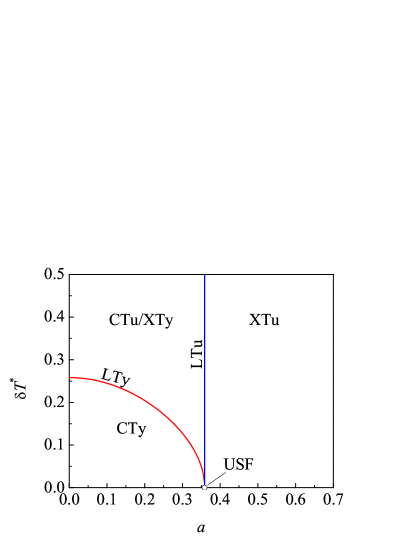
Figure 3: Phase diagram illustrating the classification of Couette–Fourier flows. This particular case corresponds to $\alpha=0.9$ and $d=3$, as obtained from Grad’s solution.

The main features of the six classes of flows described above are summarized in table 1. Note that these six profile types have been obtained independently of the specific details of the boundary conditions. Once they are specified (and they can be described more realistically than we do later in the simulations, see for instance the work by Nott et al., 1999), they will determine, for a given value of the coefficient of restitution and in the hydrodynamic bulk (i.e., the region where our four hypotheses (i)–(iv) hold), which type of profile among those in (64)–(87) the system will show.

An illustration of the phase diagram in the $a$-$\delta T^{*}$ plane at a given value of $\alpha<1$ is presented in figure 3. In fact, the LTu and LTy curves have been obtained from Grad’s solution of the Boltzmann equation (see § 4) for $\alpha=0.9$. It is apparent that the LTy class cannot be attained if $\delta T^{*}$ is larger than $2\sqrt{|\gamma(\alpha,0)|}$ ($\simeq 0.26$ in the case displayed in figure 3) or $a$ is larger than $a_{\text{LTu}}(\alpha)$ ($\simeq 0.36$ in the case displayed in figure 3). As the coefficient of restitution increases, both $|\gamma(\alpha,0)|$ and $a_{\text{LTu}}$ decrease, so that the CTu/XTy and CTy regions shrink. Of course, in the elastic case only the region XTu persists. All these features are clearly seen in the full phase diagram depicted in figure 2.

An interesting remark in the case of symmetric walls, i.e., $\delta T^{*}=0$, is the impossibility of having a temperature profile that is concave in the variables $s$ or $u_{x}$ but convex in the variable $y$ (CTu/XTy region). As figure 3 shows, if $\delta T^{*}=0$ and both plates are at rest ($a=0$), $T(y)$ is concave. As shearing is introduced and increased, the concavities of $T(y)$ and $T(u_{x})$ decrease until the value $a=a_{\text{LTu}}$ is reached, where the temperature is uniform and $u_{x}(y)$ is linear (USF). Further increase of the shearing produces convex profiles $T(y)$ and $T(u_{x})$. Thus, the existence of the ‘hybrid’ CTu/XTy region requires asymmetric walls ($\delta T^{*}\neq 0$).

6 Comparison with computer simulations

6.1 Simulation details

In this section we present the results obtained from DSMC and MD simulations for hard spheres ($d=3$) and compare them with the analytical results derived from Grad’s theory. The simulation methods that we used for DSMC and MD simulations are similar to those in our previous works and have been explained in detail elsewhere (Lobkovsky, Vega Reyes & Urbach, 2009; Vega Reyes & Urbach, 2009; Vega Reyes, Garzó & Santos, 2011a, b). We will briefly recall that DSMC yields an exact numerical solution of the corresponding kinetic equation (inelastic Boltzmann equation in this case), whereas MD yields a solution of the equations of motion of the particles. Therefore, the main difference between results from both methods is that MD simulations lack the bias of the inherent statistical approximation of the Boltzmann equation, where velocity correlations between particles which are about to collide are not considered. As in our previous work (Vega Reyes et al., 2011a), the global solid volume fraction in the MD simulations has been taken equal to $7\times 10^{-3}$ (dilute limit), using $N\sim 10^{4}$–$10^{5}$ particles. In DSMC simulations we take a similar number of particles, $N=2\times 10^{5}$. The boundary conditions used here are analogous in both methods. When a particle collides with a wall, its velocity is updated following the rule $\boldsymbol{v}\rightarrow\boldsymbol{v}^{\prime}+U_{\pm}{{\boldsymbol{e}_{x}}}$. The first contribution ($\boldsymbol{v}^{\prime}$) of the new particle velocity is due to thermal boundary condition, while the second contribution ($U_{\pm}{{\boldsymbol{e}_{x}}}$) is due to wall motion. The horizontal components of $\boldsymbol{v}^{\prime}$ are randomly drawn from a Maxwellian distribution (at a temperature $T_{\pm}$), whereas the normal component $v_{y}^{\prime}$ is sampled from a Rayleigh probability distribution: $P(|v_{y}^{\prime}|)=(m|v_{y}^{\prime}|/T_{\pm})e^{-m{v_{y}^{\prime}}^{2}/2T_{\pm}}$ (Alexander & Garcia, 1997).

At a given value of $\alpha$, we consider a common wall distance $h=15(\sqrt{2}\pi\overline{n}\sigma^{2})^{-1}$, where $\overline{n}$ is the average density, and 8 different series of simulations with $T_{+}/T_{-}=2.5$, $5.0$, $7.5$, …, $20.0$. For each value of the wall temperature ratio, a number of wall velocity differences $(U_{+}-U_{-})/\sqrt{2T_{-}/m}\approx 2$–$20$ is taken.

Once the steady state is reached, the local values of $p(y)$, $u_{x}(y)$, $T(y)$ and $\nu(y)\propto p(y)[T(y)]^{-1/2}$ are coarse-grained into $25$ layers (Vega Reyes et al., 2011b). The local shear rate $a$ is obtained from equation (25). Next, the local curvature parameters $\gamma$ and $\Phi$ are obtained from equations (53) and (57), respectively. In order to evaluate the derivatives $\partial u_{x}/\partial y$, $\partial T/\partial u_{x}$ and $\partial^{2}T/\partial u_{x}^{2}$, the profiles $u_{x}(y)$ and $T(u_{x})$ are fitted to polynomials (typically of fifth degree).

System	$\frac{U_{+}-U_{-}}{\sqrt{2T_{-}/m}}$	$\frac{T(-h/2)}{T_{-}}$	$\frac{T(h/2)}{T_{-}}$	$\frac{u_{x}(-h/2)-U_{-}}{\sqrt{2T_{-}/m}}$	$\frac{U_{+}-u_{x}(h/2)}{\sqrt{2T_{-}/m}}$	$\frac{n(-h/2)}{\overline{n}}$	$\frac{n(h/2)}{\overline{n}}$
A	$5.5$	$0.9706$	$7.1799$	$0.1892$	$0.6080$	$2.1357$	$0.2939$
B	${10.6}$	${1.2953}$	${8.9035}$	${0.2634}$	${0.8651}$	${2.8482}$	${0.4193}$
C	${11.3}$	${1.3397}$	${9.2022}$	${0.2715}$	${0.8457}$	${3.0905}$	${0.4610}$
D	$11.85$	$1.3741$	$9.3722$	$0.2727$	$0.8584$	$3.1788$	$0.4897$
E	$14.0$	$1.5154$	$10.2501$	$0.2861$	$0.8934$	$3.5821$	$0.5625$
F	$17.0$	$1.7316$	$10.9953$	$0.3062$	$0.9302$	$4.1538$	$0.6889$

Table 2: Values of the wall velocity difference and of the hydrodynamic fields near the walls for six representative systems. In all the cases $\alpha=0.9$, $h=15(\sqrt{2}\pi\overline{n}\sigma^{2})^{-1}$ and $T_{+}/T_{-}=10$.

System	$K$	$\delta T^{*}$	$a$	$\gamma$	$\Phi$	Class
A	${0.994}$	$0.1589$	$0.2491$	$-0.0110$	$\hphantom{0}0.0218$	CTy
B	${1.044}$	${0.1064}$	${0.3597}$	${-0.0022}$	${-0.00004}$	LTy
C	${1.038}$	${0.1008}$	${0.3697}$	${-0.0013}$	${-0.0049}$	CTu/XTy
D	${1.047}$	$0.0972$	$0.3753$	$-0.0006$	$-0.0087$	LTu
E	${1.062}$	$0.0854$	$0.3994$	$\hphantom{0}0.0017$	$-0.0260$	XTu
F	${1.073}$	$0.0683$	$0.4251$	$\hphantom{0}0.0044$	$-0.0558$	XTu

Table 3: Values of the parameters $K$ [equation (48)], $\delta T^{*}$ [equation (80)], $a$ [equation (25)], $\gamma$ [equation (47)] and $\Phi$ [equation (55)] for the systems described in table 2. The right-most column shows the class each system belongs to.

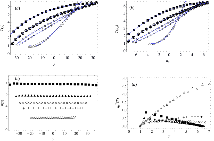
Figure 4: (a) Profile $T(y)$, (b) parametric plot $T(u_{x})$, (c) profile $\overline{p}(y)\equiv(n_{r}/\overline{n})p(y)$ and (d) parametric plot $q_{y}^{2}(T)$, as obtained from DSMC simulations for the systems A ($\triangle$), B ($+$), D ($\times$), E ($\blacktriangle$) and F ($\blacksquare$) described in table 2. Lines in (a) and (b) represent the theoretical profiles. Additionally, we present $T(y)$ and $T(u_{x})$ plots ($\bigcirc$) as obtained from MD simulations for state E. The quantities are scaled with respect to the reference units described in the text.

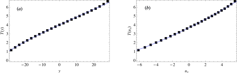
Figure 5: (a) Profile $T(y)$ and (b) parametric plot $T(u_{x})$, as obtained from DSMC simulations for the system C described in table 2. Lines represent the theoretical profiles. The quantities are scaled with respect to the reference units described in the text.

6.2 Hydrodynamic profiles

Similarly to previous works, we have observed in all simulation runs that $p$, $a$, $\gamma$ and $\Phi$ practically remain constant in the central layers of the system. Thus, in the subsequent analysis the local values of $p$, $a$, $\gamma$ and $\Phi$ are replaced by global values obtained by a spatial average in the bulk domain.

The five classes of flows summarized in table 1 and figure 3 are found in the simulations. The USF state with thermal walls, which requires $\delta T^{*}=0$, was analyzed elsewhere (Vega Reyes et al., 2010, 2011a) and is not considered here. As an illustration, let us consider the six representative systems described in table 2. We observe that, at fixed values $h=15(\sqrt{2}\pi\overline{n}\sigma^{2})^{-1}$ and $T_{+}/T_{-}=10$, the fluid temperatures near the walls do not coincide with the imposed wall values (temperature jumps). As we increase shearing, the differences $T(\pm h/2)-T_{\pm}$ increase, changing from negative to positive values (see three first columns in table 2). As for the velocity slips (Lun, 1996), i.e., the differences $u_{x}(\pm h/2)-U_{\pm}$, they also tend to increase (with one exception) with increasing shearing.

In what follows, as in former works (Vega Reyes & Urbach, 2009; Vega Reyes et al., 2011a), we take the quantities near the cold wall as reference units. Thus, $m$, $T_{r}\equiv T(-h/2)$ and $\tau_{r}\equiv 1/\nu(-h/2)$ define the units of mass, energy and time, respectively. Therefore, distances are measured in units of the nominal mean free path $\tau_{r}\sqrt{T_{r}/m}=5c_{\eta}/(16\sqrt{\pi}n_{r}\sigma^{2})$, where $n_{r}\equiv n(-h/2)$. Moreover, the density is scaled with respect to $n_{r}$. The steady-state hydrodynamic profiles for the systems in table 2 are shown in figures 4 and 5. Since the profiles in system C are very close to those of systems B and D, system C is absent in figure 4 and its temperature profiles are shown separately in figure 5. It is quite apparent that the pressure is practically uniform in all the cases, thus confirming the hypothesis (i) made in § 5. Notice also that, even though in the simulations the size is fixed at $h=15(\sqrt{2}\pi\overline{n}\sigma^{2})^{-1}$, the dimensionless size of systems A–E in the units of our choice varies since $n_{r}/\overline{n}$ is different in each case. Moreover, in our reduced units $p(y)\approx 1$ at all places and systems and so, for better visualization, in figure 4(c) we choose to plot $\overline{p}(y)$ instead. The (bulk) temperature profile $T(y)$ is concave for system A, linear for system B and convex for systems C–F. Regarding the profile $T(u_{x})$, it is concave for systems A–C, linear for system D and convex for systems E and F. The parametric dependence of $q_{y}^{2}$ versus $T$ is linear (in the bulk region) in all the cases, in agreement with equation (59), being an increasing function for systems A–C, constant for system D and decreasing for systems E and F.

The values of the quantities $K$, $\delta T^{*}$, $a$, $\gamma$ and $\Phi$ obtained from the hydrodynamic profiles of systems A–F are displayed in table 3. Notice in this table that the measured values of $\Phi$ and $\gamma$ correctly predict in all cases the observed curvatures of $T(y)$ and $T(u_{x})$, respectively. Moreover, we have obtained a very close approach to LTy and LTu states in systems B and D (for which $\Phi=-0.00004$ and $\gamma=-0.0006$. respectively).

We introduced the simulation values of $K$, $a$, $\gamma$ and $\Phi$ into the, according to our description, corresponding theoretical profiles for $T(y)$ and $T(u_{x})$, by using the pertinent (depending on the signs of $\gamma$ and $\Phi$) expressions given in § 5.3. It is worth remarking that the theoretical profiles $T(y)$ do not depend on the separate values of $K$, $a$, $\gamma$ and $\Phi$ but only on the two combinations $T_{0}$ and $\ell_{0}$ [cf. equations (62)]; as for the theoretical profiles $T(u_{x})$, they depend on the same parameter $T_{0}$ as before plus the combination $aw$. The resulting profiles are included in figures 4(a), 4(b) and 5, where the integration constants $y_{0}$ and $u_{0}$ are determined as to reproduce $T$ and $u_{x}$ at $y=0$. As we can observe, the agreement between the theoretical curves from our generalized hydrodynamic description (see § 5.3) and simulation data is excellent, the deviations typically being restricted to 1-2 layers near the cold wall and 2-4 layers near the hot wall. Those small deviations can be due to boundary-layer effects and/or to residual limitations of the hydrodynamic description exposed in § 5. In any case, it is worth remarking that the local mean free path (inversely proportional to the local density) is larger near the hot wall (where deviations present a longer range) than near the cold wall. As a matter of fact, in the employed reference units, the mean free path is $\sim 1$ near the cold wall and $\sim n(-h/2)/n(h/2)=6$–$7$ near the hot wall. It is also interesting to note that the lack of agreement near the boundaries seems to become less important as the shearing increases (i.e., from system A to system F).

The simulation data plotted in figures 4 and 5 have been obtained from the DSMC method but they perfectly agree with those obtained from MD. As an example, we compare the results obtained from both simulation methods in one of the curves of figures 4(a) and 4(b).

6.3 Transport coefficients

Once we have checked that the steady base states discussed in § 5 are supported by the simulations, we now proceed to present the simulation results for the transport coefficients and compare them with Grad’s theoretical predictions.

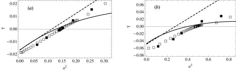
Figure 6: Thermal curvature parameter $\gamma$ as a function of shear rate squared $a^{2}$ for two values of the coefficient of restitution: (a) $\alpha=0.9$ and (b) $\alpha=0.7$. Lines represent results from Grad’s analytical solution (solid lines) and from the NS prediction (dashed lines), while symbols stand for DSMC ($\square$) and MD ($\blacksquare$) simulations.

As a general trend, we have observed a relatively good semi-quantitative agreement between simulation and Grad’s theory for all relevant quantities, except for the reduced thermal conductivity $\lambda^{*}$ and for the reduced viscosity $\eta^{*}$ at low $a$. In figure 6 we plot the results for the thermal curvature parameter $\gamma$ for two different values of the coefficient of restitution: $\alpha=0.9$ and $0.7$. We detect, both in simulations and theory, the aforementioned transition from $\gamma<0$ for low shear rates to $\gamma>0$ for higher shear rates. This transition is also predicted by the NS solution (Vega Reyes & Urbach, 2009), in which case $\gamma$ is a linear function of $a^{2}$ [see equation (28)]. As we see, the true parameter $\gamma$ has a more complex dependency on $a$. It is apparent that Grad’s theory predicts well the value $a=a_{\text{LTu}}$ where $\gamma=0$, as already shown elsewhere (Vega Reyes et al., 2010, 2011a). It is also noteworthy that, in the region $\gamma>0$, Grad’s theory does a better job for $\alpha=0.7$ than for $\alpha=0.9$. It might seem surprising that both NS and Grad’s predictions for $\gamma$ show significant discrepancies with simulation data in the region of small shear rates, especially for $\alpha=0.7$. The explanation lies in the fact that, apart from $a$ and $\delta T^{*}$, $\gamma$ is an additional measure of the strength of the gradients, which in the limit $a\to 0$ is governed by $\alpha$ and thus cannot be done arbitrarily small for finite inelasticity.

As discussed in § 5.3, for a given value of $\alpha$, it is possible to find pairs $(\delta T^{*},a)$ such that the temperature profile $T(y)$ is linear (LTy states). It is also possible to find a value of $a$, independent of $\delta T^{*}$, where the temperature profile $T(u_{x})$ is linear (LTu states). These two loci split the plane $\delta T^{*}$ vs $a$ into the three regions sketched in figure 3. We represent in figure 7 the phase diagram, as obtained from our simulations, for (a) $\alpha=0.9$ and (b) $\alpha=0.7$. For comparison, the curves predicted by Grad’s solution are also included. As we see, the agreement between theory and simulation is qualitatively good for both values of $\alpha$. As a complement, figure 8 shows the threshold value $a_{\text{LTy}}^{2}$ versus the coefficient of restitution for $\delta T^{*}=0.015$. We observe that the LTy is not possible for this value of the slope $\delta T^{*}$ if $\alpha\geq 0.967$.

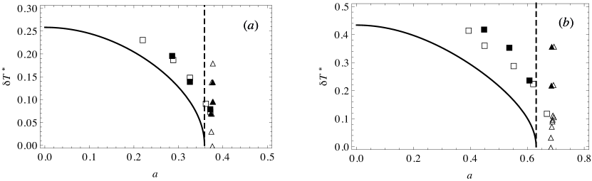
Figure 7: Phase diagram in the plane $\delta T^{*}$ vs $a$ (see figures 2 and 3) for two values of $\alpha$: (a) $\alpha=0.9$ and (b) $\alpha=0.7$. Lines stand for the analytical solution from Grad’s method, while open and solid symbols stand for DSMC and MD simulations, respectively. The LTy curve is represented by solid lines (theory) and squares (simulation), while the LTu line is represented by dashed lines (theory) and triangles (simulation).

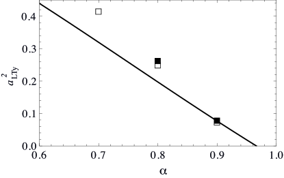
Figure 8: Threshold value $a_{\text{LTy}}^{2}$ for which the linear $T(y)$ occurs if $\delta T^{*}=0.015$, as a function of the coefficient of restitution. Line stands for Grad’s method solution, while open and solid symbols stand for DSMC and MD simulations, respectively.

In figures 9 and 10 we plot the shear-rate dependence of the reduced shear viscosity $\eta^{*}$ and of the normalized diagonal components of the stress tensor $\theta_{x}$ and $\theta_{y}$, respectively. It is quite apparent that, except for the shear viscosity in the range of low shear rates, the agreement between Grad’s analytical solution and DSMC and MD simulations is quite good (somewhat better for $\alpha=0.9$). The agreement is specially good around the LTu states (i.e., $a^{2}\approx 0.15$ and $a^{2}\approx 0.55$ for $\alpha=0.9$ and $\alpha=0.7$, respectively), as previously reported (Vega Reyes et al., 2010, 2011a). Figure 9 shows that the non-linear shear viscosity decreases with increasing shear rate (‘shear thinning’ effect). In what concerns the reduced directional temperatures, figure 10 shows that $\theta_{x}$ ($\theta_{y}$) increases (decreases) with increasing shearing. It is interesting to note that $\theta_{x}<\theta_{y}$ for very small shear rates, until both quantities cross at a certain value of $a$. This phenomenon is qualitatively captured by Grad’s solution. Comparison between figures 9(a) and 9(b) shows that, as the inelasticity decreases, the region of shear rates corresponding to $\gamma<0$, and hence the region with worse Grad’s predictions, shrinks. In fact, in the purely elastic case ($\alpha=1$) the Grad expression for $\eta^{*}$ is rather accurate (Garzó & Santos, 2003).

Finally, in figure 11 we plot the results for the two heat flux transport coefficients (thermal conductivity $\lambda^{*}$ and cross coefficient $\phi^{*}$). As already explained, there is in general a (non-Newtonian) horizontal component of the heat flux, from which the cross thermal conductivity coefficient $\phi^{*}$ results. Perhaps surprisingly, we find that the agreement between Grad’s theory and simulations is better for the cross coefficient $\phi^{*}$ than for the thermal conductivity $\lambda^{*}$. Moreover, while Grad’s theory predicts that $\lambda^{*}$ weakly increases with $a$ ($\alpha=0.9$) or exhibits a non-monotonic behavior ($\alpha=0.7$), simulations yield a decreasing $\lambda^{*}$ vs $a$. On the contrary, the agreement for the cross coefficient is qualitatively good, since $\phi^{*}$ vs $a$ is increasing both for Grad’s theory and simulation. This agreement is very good in the region of low shear rates up to the threshold value for LTu states (as expected), whereas for higher shear rates the theory and simulation results tend to separate.

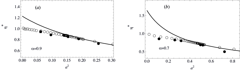
Figure 9: Generalized viscosity $\eta^{*}$ as a function of $a^{2}$ for (a) $\alpha=0.9$ and (b) $\alpha=0.7$. Lines stand for Grad’s method solution, while open and solid symbols stand for DSMC and MD simulations, respectively.

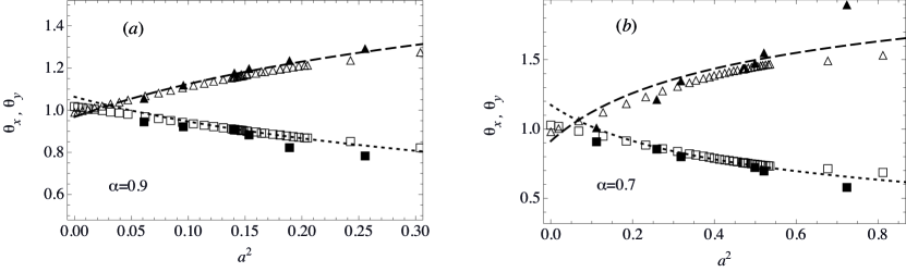
Figure 10: Reduced normal stress components $\theta_{x}$ (dashed lines and triangles) and $\theta_{y}$ (dotted lines and squares) as functions of $a^{2}$ for (a) $\alpha=0.9$ and (b) $\alpha=0.7$. Lines stand for Grad’s method solution, while open and solid symbols stand for DSMC and MD simulations, respectively.

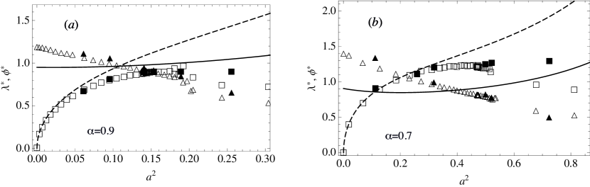
Figure 11: Generalized thermal conductivity $\lambda^{*}$ (solid lines and triangles) and heat flux cross coefficient $\phi^{*}$ (dashed lines and squares) as functions of $a^{2}$ for (a) $\alpha=0.9$ and (b) $\alpha=0.7$. Lines stand for Grad’s method solution, while open and solid symbols stand for DSMC and MD simulations, respectively.

A final comment regarding the comparison between simulation and Grad’s theory is in order. According to equation (46), $\zeta^{*}\propto k\eta^{*}a^{2}-\lambda^{*}\gamma$, where $k\equiv(d-1)/d(d+2)$. Since the reduced cooling rate $\zeta^{*}$ is satisfactorily captured by Grad’s method [(see equation (23)], we conclude that the deviations of $\eta^{*}$, $\lambda^{*}$ and $\gamma$ from the simulation data are not entirely independent and are somewhat constrained by the combination $\frac{2}{15}\eta^{*}a^{2}-\lambda^{*}\gamma$ (note that $k=\frac{2}{15}$ for $d=3$). In fact, figures 6, 9 and 11 show that, in the region with $\gamma<0$, $|\gamma|$ and $\lambda^{*}$ are underestimated by Grad’s solution, while $\eta^{*}$ is overestimated. In the region of $\gamma>0$, however, $\eta^{*}$ is quite accurate, so that the underestimation of $\gamma$ is compensated by an overestimation of $\lambda^{*}$. It is interesting to remark that the accuracy of Grad’s quantitative predictions is highly correlated with the magnitude of the thermal curvature parameter $\gamma$, i.e., the smaller $|\gamma|$ the better the general performance of Grad’s solution. In fact, the agreement between theory and simulation is quite good in the LTu state ($\gamma=0$), as previously shown by Vega Reyes et al. (2010, 2011a). This confirms the role played by $\gamma$ as an intrinsic measure of the strength of the gradients (Vega Reyes & Urbach, 2009).

7 Conclusions

Features	Level of description
	NS	Grad	Gener. non-Newton.	Simulation
(i) $p=\text{const}$	Derived	Assumed	Assumed	Observed
(ii) $a=\text{const}$	Derived	Derived	Assumed	Observed
(iii) $P_{xy}\neq F(\partial_{y}T)$	Construction	Derived	Assumed	Observed
(iv) $q_{y}\propto\partial_{y}T$	Construction	Derived	Assumed	Observed
$P_{xx}\neq P_{yy}\neq P_{zz}$	No	Yes	Yes	Yes
$q_{x}\neq 0$	No	Yes	Yes	Yes
Transport coefficients	Explicit	Explicit	Unspecified	Measured

Table 4: Hypotheses (i)–(iv) and main features of the plane Couette–Fourier flow according to the level of description: NS (§ 3), Grad’s 13-moment method (§ 4), generalized non-Newtonian hydrodynamics (§ 5) and simulation (§ 6).

7.1 Summary

We have studied in this paper the laminar flows in a low density granular gas confined between two infinite parallel walls, which, in general, are at different temperatures. Additionally, the granular gas can be sheared if there is relative motion between both walls. We have described a general classification of steady granular Couette–Fourier flows that occur in this system, at constant pressure, for arbitrarily large velocity and temperature gradients. We have shown that, due to symmetries in the system, the steady-state equations for the flow velocity and temperature are quite simple, even in the non-Newtonian regime, and have a straightforward analytical solution. Moreover, the type of solutions for the hydrodynamic profiles turn out to be dependent on just two constant parameters: the thermal curvature coefficients $\gamma$ and $\Phi$. The former is proportional to the second derivative of $T$ in a spatial variable scaled with collision frequency, while $\Phi$ is related to the second derivative in the natural spatial variable. Depending on the different possible combinations of signs of these two parameters, the corresponding steady profiles can be grouped into five different classes of flows, each one having peculiar properties (see table 1).

The main conclusions of this work are that the assumptions made on the form of the hydrodynamic profiles [see equations (25) and (41)–(44)], as well as the associated classification of flows, have been validated by three independent routes. From a theoretical perspective, we have obtained an exact solution of the set of moment equations derived from Grad’s method applied to the inelastic Boltzmann equation. Next, we have simulated the Couette–Fourier flows by using the DSMC method (which numerically solves the Boltzmann equation) and MD simulations (which numerically solve the equations of motion of the system of inelastic hard spheres).

This triple validation extends in a non-trivial way some of the qualitative features of the NS description to the realm of non-Newtonian hydrodynamics. This is summarized in table 4. As shown in § 3, the NS constitutive equations, complemented by the momentum and energy balance equations in the steady Couette–Fourier geometry, imply the fulfillment of points (i)–(iv) without further assumptions. On the other hand, they do not account for normal stress differences or a heat flux component parallel to the flow. This is remedied by Grad’s moment method, in which case only hypothesis (i) on the constancy of pressure is needed. A more general non-Newtonian treatment makes use of the four assumptions on the same footing, thus allowing us to accommodate for any specific form of the generalized transport coefficients. Finally, the simulation results are seen to support the validity of those assumptions, providing as well the dependence of the main quantities on both the shear rate and the coefficient of normal restitution. However, it must be kept in mind that, while simulations are essentially consistent to a large extent with the generalized hydrodynamic description of § 5, slight deviations due to the high intricacy of the Boltzmann equation cannot be discarded. Those small deviations have been reported in the case of the pure Fourier flow for elastic hard spheres by Montanero, Alaoui, Santos & Garzó (1994).

While Grad’s moment method supports the four assumptions (i)–(iv), as well as the existence of normal stress differences and a heat flux component orthogonal to the thermal gradient (see table 4), we have observed that a quantitative agreement with simulations is generally good near the LTu state (i.e., for small values of $|\gamma|$) only. As the magnitude of the thermal curvature parameter $\gamma$ increases, some transport coefficients ($\eta^{*}$ for $\gamma>0$, $\phi^{*}$ for $\gamma<0$ and $\theta_{x}$ and $\theta_{y}$ for both $\gamma<0$ and $\gamma>0$) are better predicted by Grad’s theory than other ones ($\eta^{*}$ for $\gamma<0$, $\phi^{*}$ for $\gamma>0$ and $\lambda^{*}$ for both $\gamma<0$ and $\gamma>0$).

7.2 Discussion

The signs of $\gamma$ and $\Phi$ depend on both the physical properties of the granular gas and the boundary conditions. However, rather than analyzing the interaction between gas and wall, our work is focused, similarly to previous works (Vega Reyes & Urbach, 2009; Vega Reyes et al., 2010), on the bulk properties of the gas itself and we study all possible transitions between the different classes of flows. All class transitions have been generated by using the usual hard wall boundary conditions, both in DSMC and MD simulations (see for instance the work by Galvin, Hrenya & Wildman, 2007, where the same boundary conditions are used for simulation of thermal walls). The phase diagram obtained from simulations is completely analogous to the theoretical one, depicted in figures 2 and 3, as shown in figure 7. We have checked in the simulations that, as in figure 2, only two of the five possible flow classes (see table 1) define surfaces in the three-parameter space $\{\alpha,\delta T^{*},a\}$. They divide this space into three regions that define three other entire classes of granular flows. Thus, we have taken these surfaces as a reference for our analysis of flow class transitions. One of the surfaces is the LTu flow class ($\gamma=0$), characterized by linear temperature vs flow velocity profiles, and already studied in former works (Vega Reyes et al., 2010, 2011a). The other surface is the LTy class ($\Phi=0$), characterized by linear temperature vs vertical coordinate profiles. The LTy surface is always below (lower shear rates) the LTu surface (figure 2), except for walls at the same temperature ($\delta T^{*}=0$ plane), where they coincide, defining a curve that is the remaining sixth flow class, which can be regarded as a subclass of the LTy or LTu classes. This class (or subclass) is actually the well known uniform shear flow (USF), i.e., constant $T$ and linear $u_{x}(y)$. Note that here the USF is achieved with thermal walls rather than with generalized periodic boundary conditions (Lees & Edwards, 1972). Regarding the other classes, the first region (CTy) is below the LTy surface and is characterized by $\gamma<0$ and $\Phi>0$. The second region (CTu/XTy) occupies the space between the LTy and LTu surfaces, being characterized with $\gamma<0$ and $\Phi<0$. Finally, the third region (XTu) is above the LTu surface and corresponds to $\gamma>0$ and $\Phi<0$ (see figure 2).

One important difference between LTy and LTu classes is that, while LTu flows are possible for arbitrarily large $\delta T^{*}$, the LTy flows are restricted to values of $\delta T^{*}$ smaller than a threshold value $\delta T^{*}_{\text{LTy}}(\alpha,a)$, which has an upper bound at $a=0$ (see figures 3 and 7). The agreement between theory and simulation in this aspect is qualitatively good. In particular, we have checked that a too large $\delta T^{*}$ in the simulations results in a direct LTu transition without passing through an LTy transition, when increasing shear rate from $a=0$. For instance, for $\alpha=0.9$, and following results in figure 7(a), a value of $\delta T^{*}=0.3$ suffices to suppress the LTy transition. Thus, in this case we would already start from $\Phi<0$ at $a=0$, never entering the class of flows with concave $T(y)$.

We have not detected so far instabilities (departures from laminar flows) in the simulations.This is reasonable since the flows that we have analyzed are either below or not far above the LTu surface, and thus they occur at low Reynolds number Re (LTu flows typically have $\mbox{{Re}}\leq 100$, see the work by Vega Reyes et al., 2011a). In order to see higher Re we would need to separate much further above the LTu surface, at extremely large shear rates, or apply larger $\delta T^{*}$.

In conclusion, we have described in detail, by means of theoretical and computational studies, all possible classes of base laminar flows for a low density granular gas in a Couette–Fourier flow geometry. Those classes differ in the curvature of the $T(y)$ and $T(u_{x})$ profiles but otherwise they can be described within a common framework characterized by a heat flux proportional to the thermal gradient and uniform stress tensor and reduced shear rate. This unified setting encompasses known and new states, from the Fourier flow of ordinary gases to the uniform shear flow of granular gases, from the symmetric Couette flow of ordinary gases to Fourier-like flows of granular gases with constant thermal gradient and from states with a magnitude of the heat flux $|\boldsymbol{q}|$ increasing with temperature to states with a decreasing, a constant or even a zero $|\boldsymbol{q}|$.

7.3 Outlook

The flow classes described in this work might be useful for future works in a variety of problems in granular dynamics, such as the study of a granular impurity under Couette flow (Garzó & Vega Reyes, 2010; Vega Reyes et al., 2011b). This implies that the same set of flow classes should exist for the granular impurity; LTu and LTy classes for instance. This may have implications to segregation conditions for a granular impurity (Jenkins & Yoon, 2002; Garzó & Vega Reyes, 2009; Garzó & Vega Reyes, 2010). Moreover, a complete determination of the steady base states is convenient for studies of instabilities (Hopkins & Louge, 1991; Wang, Jackson & Sundaresan, 1996; Alam & Nott, 1998; Nott, Alam, Agrawal, Jackson & Sundaresan, 1999; Khain & Meerson, 2003; Alam, Shukla & Luding, 2008). Furthermore, analogous temperature curvature properties are observed for the same geometry in moderately dense granular gases, except that for higher densities a region with temperature curvature inflections grows from the boundaries (Lun, 1996; Alam & Nott, 1998). Thus, we expect some of the conclusions of the present analysis to be useful for instability in quite generic problems of granular flow. We are currently working on extensions of this work in granular segregation and flow instability.

Appendix A Navier- Stokes transport coefficients

The expressions for the NS transport coefficients are (Brey et al., 1998; Brey & Cubero, 2001)

$$\eta_{\text{NS}}^{*}(\alpha)=\frac{1}{\beta_{1}(\alpha)+\frac{1}{2}\zeta^{*}(\alpha)},$$ (88)

$$\kappa_{\text{NS}}^{*}(\alpha)=\frac{1}{\beta_{2}(\alpha)-\frac{2d}{d-1}\zeta^{*}(\alpha)},$$ (89)

$$\mu_{\text{NS}}^{*}(\alpha)=\frac{\frac{d}{d-1}\zeta^{*}(\alpha)}{\left[\beta_{2}(\alpha)-\frac{2d}{d-1}\zeta^{*}(\alpha)\right]\left[\beta_{2}(\alpha)-\frac{3d}{2(d-1)}\zeta^{*}(\alpha)\right]}.$$ (90)

Here,

$$\beta_{1}(\alpha)=\frac{1+\alpha}{2}\left[1-\frac{d-1}{2d}(1-\alpha)\right],$$ (91)

$$\beta_{2}(\alpha)=\frac{1+\alpha}{2}\left[1+\frac{3}{8}\frac{d+8}{d-1}(1-\alpha)\right],$$ (92)

and the reduced cooling rate $\zeta^{*}(\alpha)$ is given by equation (23). In equations (23) and (88)–(92), terms associated with the deviation of the homogeneous cooling state distribution from a Maxwellian have been neglected (Garzó, Santos & Montanero, 2007).

Appendix B Explicit expressions in Grad’s approximation

Taking into account in equations (35)–(39) the form of the fluxes given by equations (41)–(44), one gets, after some algebra,

$$a\left[\theta_{y}-(\beta_{1}+\zeta^{*})\eta^{*}\right]-\frac{2d}{d-1}\gamma\phi^{*}=0,$$ (93)

$$(\beta_{1}+\zeta^{*})\theta_{x}-2\eta^{*}a^{2}+\frac{2d}{d-1}\gamma\lambda^{*}=\beta_{1},$$ (94)

$$(\beta_{1}+\zeta^{*})\theta_{y}+\frac{6d}{d-1}\gamma\lambda^{*}=\beta_{1},$$ (95)

$$(d+4)a\left[\eta^{*}+\frac{d}{d-1}\lambda^{*}\right]-(d+2)\beta_{2}\phi^{*}=0,$$ (96)

$$\frac{d+4}{2}\theta_{y}-\frac{d+2}{2}\beta_{2}\lambda^{*}+\frac{d}{d-1}a\phi^{*}=1.$$ (97)

The algebraic equations (93)–(97) allow one to express $\eta^{*}$, $\lambda^{*}$, $\theta_{x}$, $\theta_{y}$ and $\phi^{*}$ in terms of $a$, $\alpha$ and $\gamma$ as

$$\eta^{*} = \Delta^{-1}\left\{2d^{2}(d+4){\beta}_{1}a^{2}-(d-1)^{2}(d+2)^{2}{\beta}_{1}\beta_{2}^{2}+2d\left[d(d+4)\left((d+4)\beta_{1}-2\overline{\beta}_{1}\right)\right.\right.$$ (98)

$$\left.\left.-6(d-1)(d+2)\beta_{2}\right]\gamma\right\},$$

$$\lambda^{*}=\Delta^{-1}(d-1)\left\{\left[2\overline{\beta}_{1}-(d+4)\beta_{1}\right]\left[(d-1)(d+2)\overline{\beta}_{1}\beta_{2}+2d(d+4)\gamma\right]-2d(d+4)\beta_{1}a^{2}\right\},$$ (99)

$$\theta_{x} = (\Delta\overline{\beta}_{1})^{-1}\Big{\{}\beta_{1}(2a^{2}+\overline{\beta}_{1}^{2})\left[2d^{2}(d+4)a^{2}-(d-1)^{2}(d+2)^{2}\beta_{2}^{2}\right]+2d\left[2d(d+4)a^{2}\right.$$ (100)

$$\left.\times\left((d+2)\beta_{1}-2\overline{\beta}_{1}\right)-(d-1)(d+2)\beta_{2}\left(12a^{2}+\overline{\beta}_{1}\left(2\overline{\beta}_{1}+3(d+4)\beta_{1}\right)\right)\right]\gamma$$

$$-8d^{2}(d+4)\left[\overline{\beta}_{1}+(d+4)\beta_{1}\right]\gamma^{2}\Big{\}},$$

$$\theta_{y} = \Delta^{-1}\Big{\{}2d^{2}(d+4)\overline{\beta}_{1}\beta_{1}a^{2}-\left[(d-1)(d+2){\beta}_{1}\beta_{2}+12d\gamma\right]$$ (101)

$$\times\left[(d-1)(d+2)\overline{\beta}_{1}\beta_{2}+2d(d+4)\gamma\right]\Big{\}},$$

$$\phi^{*}=\Delta^{-1}(d-1)(d+4)a\left\{d\overline{\beta}_{1}\left[2\overline{\beta}_{1}-(d+4){\beta}_{1}\right]-(d-1)(d+2){\beta}_{1}\beta_{2}-12d\gamma\right\},$$ (102)

where $\overline{\beta}_{1}\equiv\beta_{1}+\zeta^{*}$ and

$$\Delta \equiv 2d^{2}(d+4)(\overline{\beta}_{1}^{2}-6\gamma)a^{2}-(d-1)^{2}(d+2)^{2}\overline{\beta}_{1}^{2}\beta_{2}^{2}-8d(d-1)(d+2)(d+4)\overline{\beta}_{1}\beta_{2}\gamma$$ (103)

$$-12d^{2}(d+4)^{2}\gamma^{2}.$$

Finally, substitution of $\eta^{*}$ and $\lambda^{*}$ into equation (46) yields a quadratic equation for $\gamma$. Its physical solution gives $\gamma$ as a function of the shear rate $a$ and the coefficient of restitution $\alpha$.

Setting $\gamma=0$ in equations (46), (98) and (99), we get the prediction for the LTu threshold shear rate in Grad’s approximation. The result is

$$a_{\text{LTu}}(\alpha)=\sqrt{\frac{d\zeta^{*}}{2\beta_{1}}}\overline{\beta}_{1}.$$ (104)

The expressions for the LTu transport coefficients $\eta^{*}$, $\lambda^{*}$, $\theta_{x}$, $\theta_{y}$ and $\phi^{*}$ are obtained by making $a=a_{\text{Ltu}}$ and $\gamma=0$ in equations (98)–(103). The explicit expressions have been given elsewhere (Vega Reyes et al., 2011a).

In the absence of shearing ($a\to 0$), equations (46) and (98)–(103) yield

$$\gamma^{*}=-\frac{(d+2)(d-1)\beta_{2}\zeta^{*}\overline{\beta}_{1}}{2\left[(d+2)^{2}\beta_{1}+(3d^{2}+10d-4)\zeta^{*}\right]},$$ (105)

$$\eta^{*} = \frac{(d+2)^{2}\beta_{1}+(3d^{2}+10d-4)\zeta^{*}}{(d+2)^{2}\beta_{1}+2(d^{2}+3d-2)\zeta^{*}}\Big{\{}\beta_{1}\left[(d+2)^{2}(d-1)\beta_{2}+d^{2}(d+4)\zeta^{*}\right]$$ (106)

$$+d\zeta^{*}\left[3(d+2)(d-1)\beta_{2}+d(d+4)\zeta^{*}\right]\Big{\}}/{(d-1)(d+2)^{2}\beta_{2}\overline{\beta}_{1}^{2}},$$

$$\lambda^{*}=\frac{(d+2)^{2}\beta_{1}+(3d^{2}+10d-4)\zeta^{*}}{(d+2)^{2}\beta_{2}\overline{\beta}_{1}},$$ (107)

$$\theta_{x}=\frac{(d+2)\beta_{1}+d\zeta^{*}}{(d+2)\overline{\beta}_{1}},$$ (108)

$$\theta_{y}=\frac{(d+2)\beta_{1}+3d\zeta^{*}}{(d+2)\overline{\beta}_{1}},$$ (109)

$$\frac{\phi^{*}}{a} = \frac{d+4}{(d-1)(d+2)^{3}\beta_{2}^{2}\overline{\beta}_{1}^{2}}\frac{(d+2)^{2}\beta_{1}+(3d^{2}+10d-4)\zeta^{*}}{(d+2)^{2}\beta_{1}+2(d^{2}+3d-2)\zeta^{*}}\Big{\{}d(d+2)^{2}\beta_{1}^{2}+\beta_{1}\left[(d+2)^{2}\right.$$

$$\left.\times(d-1)\beta_{2}+2d^{2}(2d+7)\zeta^{*}\right]+d\zeta^{*}\left[3(d+2)(d-1)\beta_{2}+(3d^{2}-10d+4)\zeta^{*}\right]\Big{\}}.$$

In the elastic case ($\zeta^{*}\to 0$, $\beta_{1}\to 1$, $\beta_{2}\to 1$), one has $\theta_{x}\to 1$, $\theta_{y}\to 1$, $\lambda^{*}\to 1$, $\eta^{*}\to 1$, $\gamma\to 0$ and $\phi^{*}/a\to(2d-1)(d+4)/(d-1)(d+2)$, which corresponds to the Fourier flow of conventional gases.

References

- Agarwal et al. (2001) Agarwal, R. K., Yun, K.-Y. & Balakrishnan, R. 2001 Beyond Navier-Stokes: Burnett equations for flows in the continuum transition regime. Phys. Fluids 13, 3061–3085.
- Alam et al. (2005) Alam, M., Arakeri, V. H., Nott, P. R., Goddard, J. D. & Herrmann, H. J. 2005 Instability-induced ordering, universal unfolding and the role of gravity in granular Couette flow. J. Fluid Mech. 523, 277–306.
- Alam & Chikkadi (2010) Alam, M. & Chikkadi, V. K. 2010 Velocity distribution function and correlations in a granular Poiseuille flow. J. Fluid Mech. 653, 175–219.
- Alam & Luding (2003) Alam, M. & Luding, S. 2003 Rheology of bidisperse granular mixtures via event-driven simulations. J. Fluid Mech. 476, 69–103.
- Alam & Nott (1998) Alam, M. & Nott, P. 1998 Stability of plane Couette flow of a granular material. J. Fluid Mech. 377, 99–136.
- Alam et al. (2008) Alam, M., Shukla, P. & Luding, S. 2008 Universality of shear-banding instability and crystallization in sheared granular fluid. J. Fluid Mech. 615, 293–321.
- Alexander & Garcia (1997) Alexander, F. J. & Garcia, A. L. 1997 The direct simulation Monte Carlo method. Comp. Phys. 11, 588–593.
- Aranson & Tsimring (2006) Aranson, I. S. & Tsimring, L. S. 2006 Patterns and collective behavior in granular media: Theoretical concepts. Rev. Mod. Phys. 78, 641–692.
- Astillero & Santos (2005) Astillero, A. & Santos, A. 2005 Uniform shear flow in dissipative gases: Computer simulations of inelastic hard spheres and frictional elastic hard spheres. Phys. Rev. E 72, 031309.
- Brey & Cubero (1998) Brey, J. J. & Cubero, D. 1998 Steady state of a fluidized granular medium betwen two walls at the same temperature. Phys. Rev. E 57, 2019–2029.
- Brey & Cubero (2001) Brey, J. J. & Cubero, D. 2001 Hydrodynamic transport coefficients of granular gases. In Granular Gases (ed. T. Pöschel & S. Luding), Lectures Notes in Physics, vol. 564, pp. 59–78. Berlin: Springer.
- Brey et al. (2001) Brey, J. J., Cubero, D., Moreno, F. & Ruiz-Montero, M. J. 2001 Fourier state of a fluidized granular gas. Europhys. Lett. 53, 432–437.
- Brey et al. (1998) Brey, J. J., Dufty, J. W., Kim, C. S. & Santos, A. 1998 Hydrodynamics for granular flow at low density. Phys. Rev. E 58, 4638–4653.
- Brey et al. (2011) Brey, J. J., Khalil, N. & Dufty, J. W 2011 Thermal segregation beyond Navier–Stokes. New J. Phys. 13, 055019.
- Brey et al. (2012) Brey, J. J., Khalil, N. & Dufty, J. W 2012 Thermal segregation of intruders in the Fourier state of a granular gas. Phys. Rev. E 85, 021307.
- Brey et al. (2009) Brey, J. J., Khalil, N. & Ruiz-Montero, M. J. 2009 The Fourier state of a dilute granular gas described by the inelastic Boltzmann equation. J. Stat. Mech. p. P08019.
- Brey et al. (2000) Brey, J. J., Ruiz-Montero, M. J. & Moreno, F. 2000 Boundary conditions and normal state for a vibrated granular fluid. Phys. Rev. E 62, 5339–5346.
- Brilliantov & Pöschel (2004) Brilliantov, N. V. & Pöschel, T. 2004 Kinetic Theory of Granular Gases. Oxford University Press, Oxford.
- Brilliantov et al. (2007) Brilliantov, N. V., Pöschel, T., Kranz, W. T. & Zippelius, A. 2007 Translations and rotations are correlated in granular gases. Phys. Rev. Lett. 98, 128001.
- Burnett (1935) Burnett, D. 1935 The distribution of velocities in a slightly non-uniform gas. Proc. London Math. Soc. 39, 385–430.
- Campbell (1989) Campbell, C. S. 1989 The stress tensor for simple shear flows of a granular material. J. Fluid Mech. 203, 449–473.
- Cercignani (1988) Cercignani, C. 1988 The Boltzmann Equation and Its Applications. New York: Springer–Verlag.
- Chapman & Cowling (1970) Chapman, C. & Cowling, T. G. 1970 The Mathematical Theory of Non-Uniform Gases, 3rd edn. Cambridge University Press, Cambridge.
- Dahl et al. (2002) Dahl, S. R., Hrenya, C. M., Garzó, V. & Dufty, J. W. 2002 Kinetic temperatures for a granular mixture. Phys. Rev. E 66, 041301.
- Galvin et al. (2007) Galvin, J. E., Hrenya, C. M. & Wildman, R. D. 2007 On the role of the Knudsen layer in rapid granular flows. J. Fluid Mech. 585, 73–92.
- Garzó & Montanero (2002) Garzó, V. & Montanero, J. M. 2002 Transport coefficients of a heated granular gas. Physica A 313, 336–356.
- Garzó & Santos (2003) Garzó, V. & Santos, A. 2003 Kinetic Theory of Gases in Shear Flows. Nonlinear Transport. Dordrecht: Kluwer Academic.
- Garzó et al. (2007) Garzó, V., Santos, A. & Montanero, J. M. 2007 Modified Sonine approximation for the Navier–Stokes transport coefficients of a granular gas. Physica A 376, 94–107.
- Garzó & Vega Reyes (2009) Garzó, V. & Vega Reyes, F. 2009 Mass transport of impurities in a moderately dense granular gas. Phys. Rev. E 79, 041303.
- Garzó & Vega Reyes (2010) Garzó, V. & Vega Reyes, F. 2010 Segregation by thermal diffusion in granular shear flows. J. Stat. Mech. p. P07024.
- Goldhirsch (2003) Goldhirsch, I. 2003 Rapid granular flows. Annu. Rev. Fluid Mech. 35, 267–293.
- Goldhirsch & Zanetti (1993) Goldhirsch, I. & Zanetti, G. 1993 Clustering instability in dissipative gases. Phys. Rev. Lett. 70, 1619–1622.
- Grad (1949) Grad, H. 1949 On the kinetic theory of rarefied gases. Commun. Pure Appl. Math. 2, 331–407.
- Grossman et al. (1997) Grossman, E. L., Zhou, T. & Ben-Naim, E. 1997 Towards granular hydrodynamics in two dimensions. Phys. Rev. E 55, 4200.
- Haff (1983) Haff, P. K. 1983 Grain flow as a fluid-mechanical phenomenon. J. Fluid Mech. 134, 401–430.
- Herdegen & Hess (1982) Herdegen, N. & Hess, S. 1982 Nonlinear flow behavior of the Boltzmann gas. Physica A 115, 281–299.
- Hilbert (1912) Hilbert, D. 1912 Begründung der kinetischen Gastheorie. Math. Ann. 72, 562–577.
- Hopkins & Louge (1991) Hopkins, M. A. & Louge, M. Y. 1991 Inelastic microstructure in rapid granular flows of smooth disks. Phys. Fluids A 3, 47–57.
- Huang (1987) Huang, K. 1987 Statistical Mechanics. New York: John Wiley.
- Jenkins & Savage (1983) Jenkins, J. T. & Savage, S. B. 1983 A theory for the rapid flow of identical, smooth, nearly elastic, spherical spheres. J. Fluid Mech. 130, 187–202.
- Jenkins & Yoon (2002) Jenkins, J. T. & Yoon, D. K. 2002 Segregation in binary mixtures under gravity. Phys. Rev. Lett. 88, 194301.
- Khain & Meerson (2003) Khain, E. & Meerson, B. 2003 Onset of thermal convection in a horizontal layer of granular gas. Phys. Rev. E 67, 021306.
- Kolvin et al. (2010) Kolvin, I., Livne, E. & Meerson, B. 2010 Navier-Stokes hydrodynamics of thermal collapse in a freely cooling granular gas. Phys. Rev. E 82, 021302.
- Kremer (2010) Kremer, G. M. 2010 An Introduction to the Boltzmann Equation and Transport Processes in Gases. Springer.
- Lees & Edwards (1972) Lees, A. W. & Edwards, S. F. 1972 The computer study of transport processes under extreme conditions. J. Phys. C 5, 1921–1929.
- Lobkovsky et al. (2009) Lobkovsky, A. E., Vega Reyes, F. & Urbach, J. S. 2009 The effects of forcing and dissipation on phase transitions in thin granular layers. Eur. Phys. J. Spec. Top. 179, 113.
- Lun (1996) Lun, C. K. K. 1996 Granular dynamics of inelastic spheres in Couette flow. Phys. Fluids 8, 2868–2883.
- Lutsko et al. (2002) Lutsko, J., Brey, J. J. & Dufty, J. W. 2002 Diffusion in a granular fluid. II. Simulation. Phys. Rev. E 65, 051304.
- McNamara & Luding (1998) McNamara, S. & Luding, S. 1998 Energy non-equipartition in systems of inelastic, rough spheres. Phys. Rev. E 58, 2247–2250.
- Montanero et al. (1994) Montanero, J. M., Alaoui, M., Santos, A. & Garzó, V. 1994 Monte Carlo simulation of the Boltzmann equation for steady Fourier flow. Phys. Rev. A 49, 367–375.
- Montanero et al. (2006) Montanero, J. M., Garzó, V., Alam, M. & Luding, S. 2006 Rheology of two- and three-dimensional granular mixtures under uniform shear flow: Enskog kinetic theory versus molecular dynamics simulations. Gran. Matt. 8, 103–115.
- Montanero et al. (1998) Montanero, J. M., López de Haro, M., Garzó, V. & Santos, A. 1998 Strong shock waves in a dense gas: Burnett theory versus Monte Carlo simulation. Phys. Rev. E 58, 7319–7324.
- Montanero et al. (1999) Montanero, J. M., López de Haro, M., Santos, A. & Garzó, V. 1999 Simple and accurate theory for strong shock waves in a dense hard-sphere fluid. Phys. Rev. E 60, 7592–7595.
- Nott (2011) Nott, P. R. 2011 Boundary conditions at a rigid wall for rough granular gases. J. Fluid Mech. 678, 179–202.
- Nott et al. (1999) Nott, P. R., Alam, M., Agrawal, K., Jackson, R. & Sundaresan, S. 1999 The effect of boundaries on the plane Couette flow of granular materials: a bifurcation analysis. J. Fluid Mech. 397, 203–229.
- Pagonabarraga et al. (2002) Pagonabarraga, I., Trizac, E., van Noije, T. P. C. & Ernst, M. H. 2002 Randomly driven granular fluids: collisional statistics and short scale structure. Phys. Rev. E 65, 011303.
- Prevost et al. (2002) Prevost, A., Egolf, D. E. & Urbach, J. S. 2002 Forcing and velocity correlations in a vibrated granular monolayer. Phys. Rev. Lett. 89, 084301.
- Santos et al. (2004) Santos, A., Garzó, V. & Dufty, J. W. 2004 Inherent rheology of a granular fluid in uniform shear flow. Phys. Rev. E 69, 061303.
- Santos et al. (2009) Santos, A., Garzó, V. & Vega Reyes, F. 2009 An exact solution of the inelastic Boltzmann equation for the Couette flow with uniform heat flux. Eur. Phys. J. Spec. Top. 179, 141–156.
- Santos & Tij (2006) Santos, A. & Tij, M. 2006 Gravity-driven Poiseuille Flow in Dilute Gases. Elastic and Inelastic Collisions. In Modelling and Numerics of Kinetic Dissipative Systems (ed. L. Pareschi, G. Russo & G. Toscani), pp. 53–67. New York: Nova Science Publishers.
- Schlamp & Hathorn (2007) Schlamp, S. & Hathorn, B. C. 2007 Incomplete molecular chaos within dense-fluid shock waves. Phys. Rev. E 76, 026314.
- Sela & Goldhirsch (1998) Sela, N. & Goldhirsch, I. 1998 Hydrodynamic equations for rapid flows of smooth inelastic spheres, to Burnett order. J. Fluid Mech. 361, 41–74.
- Soto & Mareschal (2001) Soto, R. & Mareschal, M. 2001 Statistical mechanics of fluidized granular media: Short-range velocity correlations. Phys. Rev. E 63, 041303.
- Soto et al. (2001) Soto, R., Piasecki, J. & Mareschal, M. 2001 Precollisional velocity correlations in a hard-disk fluid with dissipative collisions. Phys. Rev. E 64, 031306.
- Tij & Santos (2004) Tij, M. & Santos, A. 2004 Poiseuille flow in a heated granular gas. J. Stat. Phys. 117, 901–928.
- Tij et al. (2001) Tij, M., Tahiri, E. E., Montanero, J. M., Garzó, V., Santos, A. & Dufty, J. W. 2001 Nonlinear Couette flow in a low density granular gas. J. Stat. Phys. 103, 1035–1068.
- Tsao & Koch (1995) Tsao, H.-K. & Koch, D. L. 1995 Simple shear flows of dilute gas-solid suspensions. J. Fluid Mech. 296, 211–245.
- Vega Reyes et al. (2011a) Vega Reyes, F., Garzó, V. & Santos, A. 2011a Class of dilute granular Couette flows with uniform heat flux. Phys. Rev. E 83, 021302.
- Vega Reyes et al. (2010) Vega Reyes, F., Santos, A. & Garzó, V. 2010 Non-Newtonian granular hydrodynamics. What do the inelastic simple shear flow and the elastic Fourier flow have in common? Phys. Rev. Lett. 104, 028001.
- Vega Reyes et al. (2011b) Vega Reyes, F., Santos, A. & Garzó, V. 2011b Computer simulations of an impurity in a granular gas under planar Couette flow. J. Stat. Mech. p. P07005.
- Vega Reyes & Urbach (2009) Vega Reyes, F. & Urbach, J. S. 2009 Steady base states for Navier-Stokes granular hydrodynamics with boundary heating and shear. J. Fluid Mech. 636, 279–293.
- Wang et al. (1996) Wang, C.-W., Jackson, R. & Sundaresan, S. 1996 Stability of bounded rapid shear flows of a granular material. J. Fluid Mech. 308, 31–62.