Efficiency of a Brownian information machine

Abstract

A Brownian information machine extracts work from a heat bath through a feedback process that exploits the information acquired in a measurement. For the paradigmatic case of a particle trapped in a harmonic potential, we determine how power and efficiency for two variants of such a machine operating cyclically depend on the cycle time and the precision of the positional measurements. Controlling only the center of the trap leads to a machine that has zero efficiency at maximum power whereas additional optimal control of the stiffness of the trap leads to an efficiency bounded between 1/2, which holds for maximum power, and 1 reached even for finite cycle time in the limit of perfect measurements.

In Kelvin’s formulation, the second law of thermodynamics states that no work can be extracted from a thermally equilibrated system through a cyclic process that leaves no trace elsewhere. If, however, more detailed information of the system becomes available through a measurement, then one can indeed extract work as illustrated a long time ago with the gedankenexperiments of Maxwell’s demon and Szilard’s engine [1]. More recently, by combining concepts from stochastic thermodynamics with those from information theory, a quantitative framework has emerged leading to bounds refining the second law to such feedback driven processes [2, 3, 4, 5, 6, 7, 8, 9, 10]. Specialized to one cyclic process starting in equilibrium, the bound

$$W\leq{\cal I}$$ (1)

connects the mean extractable work $W$ to the mean information ${\cal I}$ (defined more precisely below) acquired through the measurement. Brownian particles in time-dependent potentials provide a paradigm for such systems both in recent experiments [11, 12] as in several theoretical case studies [13, 14, 15]. The latter works have demonstrated that saturating the bound in (1) typically requires both an infinite cycle time and a sufficient number of control parameters in the potential.

The purpose of the present paper is to study these processes from a perspective that focuses on the performance of such Brownian information machines in a steady state where measurements and subsequent optimal driving based on these are repeated with a finite cycle time $t$. On average per cycle, by exploiting the information ${\cal I}_{*}$, the machine extracts the work $W_{*}$ thus delivering a power $P\equiv W_{*}/t$. The extant generalization of the bound (1) to such a cyclic operation [8] then motivates to define efficiency as

$$\eta\equiv W/{\cal I}$$ (2)

following in spirit an earlier approach [4]. Apart from maximum efficiency, it is particularly interesting to determine efficiency at maximum power. The later concept has been studied extensively for non-feedback driven heat engines operating between two heat baths, see, e.g., [16, 17, 18, 19] and references therein, and, more recently, also for autonomous isothermal machines [20].

The solution to this problem of performance at a finite cycle time cannot trivially be inferred from available results [14] on the maximal extractable work following one measurement in finite time since at the beginning of the second (and any further) cycle the system will typically not have reached thermal equilibrium again. In fact, the initial state of the $i-$th-cycle will depend on the result of all previous measurements which makes the present problem non-trivial.

Our system consists of an overdamped Brownian particle in a harmonic potential

$$V(x,\tau)=k(\tau)[x-\lambda(\tau)]^{2}/2$$ (3)

with external time-dependent control of the center, $\lambda(\tau)$, and stiffness, $k(\tau)$, of the trap [14]. Throughout the paper, we use dimensionless variables. The harmonic potential has the advantage that a Gaussian distribution

$$p(x)={\cal N}_{x}(b,y^{2})\equiv\frac{1}{(2\pi)^{1/2}y}\exp\left(-\frac{(x-b)^{2}}{2y^{2}}\right)$$ (4)

remains Gaussian both under the stochastic dynamics in the potential and under positional measurements with an error $\pm~{}y_{m}$. The dynamics of the mean $b(\tau)$ and variance $y^{2}(\tau)$ of $x$ follows from the corresponding Fokker-Planck equation as [14]

$$\dot{b}(\tau)=k(\tau)[\lambda(\tau)-b(\tau)]$$ (5)

and

$$\dot{y}(\tau)=y(\tau)[1/y^{2}(\tau)-k(\tau)]$$ (6)

where we denote time-derivatives with a dot throughout.

We now implement a cyclic feedback scheme based on measurements of the position repeated periodically in intervals of lengths $t$. At the beginning of the $i-$th cycle, we measure the position $X_{i}$ with a precision $\pm~{}y_{m}$ leading to the distribution

$$p(X_{i})={\cal N}_{X_{i}}({b_{i}^{-}},{(y_{i}^{-})}^{2}+y_{m}^{2})$$ (7)

for the measured value if the distribution prior to the measurement is characterized by

$$p_{i}^{-}(x)={\cal N}_{x}({b_{i}^{-}},{(y_{i}^{-})}^{2}).$$ (8)

After the measurement the distribution for $x$ follows from Bayes’ theorem as

$$p(x|X_{i})={\cal N}_{x}({b_{i}^{+}},{(y_{i}^{+})}^{2}),$$ (9)

with

$${b_{i}^{+}}=\frac{X_{i}{(y_{i}^{-})}^{2}+{b_{i}^{-}}y_{m}^{2}}{{(y_{i}^{-})}^{2}+y_{m}^{2}}$$ (10)

and

$${(y_{i}^{+})}^{2}=\frac{{(y_{i}^{-})}^{2}y_{m}^{2}}{{(y_{i}^{-})}^{2}+y_{m}^{2}}.$$ (11)

Based on this measurement, we maximize the extracted work by optimally adjusting the control parameters. Quite generally, given an initial state ${b(0)={b_{i}^{+}},y^{2}(0)={(y_{i}^{+})}^{2}}$ and a time-dependent $b(\tau)$ and $y(\tau)$, the extracted work after a time $t$ becomes [14]

$$W^{\rm out}=W^{\rm out}_{b}+W^{\rm out}_{y}$$ (12)

with

$$-W^{\rm out}_{b}\equiv[b^{2}(t)-({b_{i}^{+}})^{2}]/2+\int_{0}^{t}d\tau~{}\dot{b}^{2}(\tau)$$ (13)

and

$$-W^{\rm out}_{y}\equiv[y^{2}(t)-{(y_{i}^{+})}^{2}]/2-\ln[y(t)/y_{i}^{+}]+\int_{0}^{t}d\tau~{}\dot{y}^{2}(\tau).$$ (14)

Here, we have required that the trap is centered at $\lambda=0$ with stiffness $k=1$ at beginning and end of the cycle allowing for jumps of these two control parameters. Depending on the amount of control available, two cases must be distinguished.

If the stiffness is fixed, $k(\tau)\equiv 1$, only the center of the trap $\lambda(\tau)$ is controllable. Using (6) in the integral (14) shows that in this case $W^{\rm out}_{y}\equiv 0$. The $b$-dependent term is maximized by a linear function $b(\tau)={b_{i}^{+}}[1-\tau/(2+t)]$ leading to the optimal extracted work in the $i$-th cycle

$$W_{i}^{\rm out}=({b_{i}^{+}})^{2}t/[2(2+t)].$$ (15)

This work still depends on the result of all measurements $\{X_{j}\}_{1\leq j\leq i}$. Conditionally averaging this work over the last measurement will lead to a useful recursion relation as follows. With

$$\langle({b_{i}^{+}})^{2}\rangle_{{X_{i}}}\equiv\int dX_{i}~{}({b_{i}^{+}})^{2}p(X_{i})$$ (16)

and (7), (10) and (11) we get

$$\langle({b_{i}^{+}})^{2}\rangle_{{X_{i}}}=\frac{4}{(2+t)^{2}}{(b_{i-1}^{+}})^{2}+{(y_{i}^{-})}^{2}-{(y_{i}^{+})}^{2}$$ (17)

and hence

$$\langle W_{i}^{\rm out}\rangle_{{X_{i}}}=\frac{4}{(2+t)^{2}}W_{i-1}^{\rm out}+\frac{t}{2(2+t)}\left({(y_{i}^{-})}^{2}-{(y_{i}^{+})}^{2}\right).$$ (18)

Since the last term is independent of the outcomes of measurements, subsequent averaging over all previous measurements $\{X_{j}\}_{1\leq j\leq i-1}$ (indicated by an unconstrained bracket $\langle...\rangle$) leads to

$$\langle W_{i}^{\rm out}\rangle=\frac{4}{(2+t)^{2}}\langle W_{i-1}^{\rm out}\rangle+\frac{t}{2(2+t)}\left({(y_{i}^{-})}^{2}-{(y_{i}^{+})}^{2}\right).$$ (19)

Solving this recursion in the stationary limit, $i\to\infty$, we thus obtain as the average work per cycle

$$W_{*}\equiv\lim_{i\to\infty}\langle W_{i}^{\rm out}\rangle=\frac{2+t}{2(4+t)}\lim_{i\to\infty}\left({(y_{i}^{-})}^{2}-{(y_{i}^{+})}^{2}\right).$$ (20)

The last limit is easily calculated by solving the dynamics (6) for the variance as

$$y^{2}(\tau)=1+e^{-2\tau}[y^{2}(0)-1]$$ (21)

and setting $y^{2}(t)=(y_{i+1}^{-})^{2}$ and $y^{2}(0)={(y_{i}^{+})}^{2}$. Using (11), and identifying $y_{i+1}^{-}$ with $y_{i}^{-}$ in the limit $i\to\infty$, we get in the steady state for the variance before a measurement the value

$$({y^{-}_{*}})^{2}\equiv\lim_{i\to\infty}{(y_{i}^{-})}^{2}=\frac{1}{2}\bigg{(} 1-y_{m}^{2}+e^{-2t}(y_{m}^{2}-1)$$

$$+\sqrt{(y_{m}^{2}+1)^{2}-2e^{-2t}(y_{m}^{4}+1)+e^{-4t}(y_{m}^{2}-1)^{2}}\bigg{)}$$

with the limiting behavior

$$(y_{*}^{-})^{2}\approx\left\{\begin{array}[]{l l}y_{m}(2t)^{1/2}+(1-y_{m}^{2})t&{\rm~{}~{}~{}for~{}~{}~{}}t\to 0\\ 1-\exp(-2t)/(1+y_{m}^{2})&{\rm~{}~{}~{}for~{}~{}~{}}t\to\infty.\end{array}\right.$$ (25)

Likewise, the variance after a measurement becomes

$$({y_{*}^{+}})^{2}\equiv\lim_{i\to\infty}{(y_{i}^{+})}^{2}=\frac{({y^{-}_{*}})^{2}y_{m}^{2}}{({y^{-}_{*}})^{2}+y_{m}^{2}}$$ (26)

with the limiting behavior

$$(y_{*}^{+})^{2}\approx\left\{\begin{array}[]{l l}y_{m}(2t)^{1/2}-(1+y_{m}^{2})t&{\rm~{}~{}~{}for~{}~{}~{}}t\to 0\\ {\displaystyle\frac{y_{m}^{2}}{1+y_{m}^{2}}\left(1-\exp(-2t)\frac{y_{m}^{2}}{(1+y_{m}^{2})^{2}}\right)}&{\rm~{}~{}~{}for~{}~{}~{}}t\to\infty.\end{array}\right.$$ (29)

Finally, the average work per cycle delivered by this information machine becomes

$$W_{*}=\frac{2+t}{2(4+t)}\left((y^{-}_{*})^{2}-(y_{*}^{+})^{2}\right)$$ (30)

which is our first main result, shown in Fig. 1. The power $P\equiv W_{*}/t$ becomes maximal if the cycle time becomes short with $P\approx 1/2-y_{m}(t/2)^{1/2}$ for $t\to 0$. In the long time limit, $P\approx 1/[2t(1+y_{m}^{2})]$ for $t\to\infty$. In the special case of an infinitely precise measurement, we get $P(t,0)=(1-e^{-2t})(2+t)/[2t(4+t)]$.

The efficiency of this machine follows from relating the power to the rate with which information is acquired through the measurements. The $i$-th measurement yields the information [5]

$${\scriptstyle{\cal I}}_{i}=\int dxp(x|X_{i})\ln[p(x|X_{i})/p_{i}^{-}(x)],$$ (31)

which still depends on the result of all measurements $\{X_{j}\}_{1\leq j\leq i}$. By using (8) and (9), subsequent averaging over the last measurement $X_{i}$ yields

$${\cal I}_{i}\equiv\int dX_{i}~{}p(X_{i}){\scriptstyle{\cal I}}_{i}=\ln(y_{i}^{-}/y_{i}^{+}).$$ (32)

This simple result involves, a posteriori not surprisingly, just the variances before and after the measurement which are independent of the specific results $\{X_{j}\}_{1\leq j\leq i-1}$. ${\cal I}_{i}$ thus represents the information averaged over all measurement outcomes. In the stationary limit, one gets

$${\cal I}_{*}\equiv\ln(y^{-}_{*}/y^{+}_{*})\approx\left\{\begin{array}[]{l l}(t/2)^{1/2}/y_{m}-t/2&{\rm~{}~{}~{}for~{}~{}~{}}t\to 0\\ {\displaystyle\frac{1}{2}\ln\left(1+\frac{1}{y_{m}^{2}}\right)-\frac{\exp(-2t)}{2(1+y_{m}^{2})^{2}}}&{\rm~{}~{}~{}for~{}~{}~{}}t\to\infty.\end{array}\right.$$ (35)

Consequently, the efficiency becomes

$$\eta\equiv W_{*}/{\cal I}_{*}=\frac{(2+t)\left((y^{-}_{*})^{2}-(y_{*}^{+})^{2}\right)}{2(4+t)\ln(y_{*}^{-}/y_{*}^{+})}$$ (36)

with the limiting behaviour

$$\eta\approx\left\{\begin{array}[]{l l}y_{m}(t/2)^{1/2}-y_{m}^{2}t/2&{\rm~{}~{}~{}for~{}~{}~{}}t\to 0\\ {\displaystyle\frac{1-2/t}{(1+y_{m}^{2})\ln(1+1/y_{m}^{2})}}&{\rm~{}~{}~{}for~{}~{}~{}}t\to\infty.\end{array}\right.$$ (39)

As shown in Fig. 1, the efficiency increases monotonically with the cycle time $t$. It becomes zero for $t\to 0$, which implies that this machine has vanishing efficiency at maximum power. The somewhat counterintuitive monotonic increase of $\eta$ with the measurement error $y_{m}$ arises from the fact that it is impossible to retrieve all information just by moving the center of the trap. Therefore, better measurements lead to a higher power but not to a higher efficiency. Indeed, while the work $W_{*}$ is bounded by $1/2$ [14], the information ${\cal I}_{*}$ diverges in the limit of infinitely precise measurements $y_{m}\to 0$, leading to a vanishing efficiency. In the limit $y_{m}\to\infty$, both $W_{*}$ and ${\cal I}_{*}$ tend to 0 and $\eta\to(2+t)/(4+t)$. For $t\to\infty$, this machine can reach the upper bound 1 imposed on $\eta$ by thermodynamics. However, this high efficiency is somewhat useless, since in this case the machine delivers vanishing power.

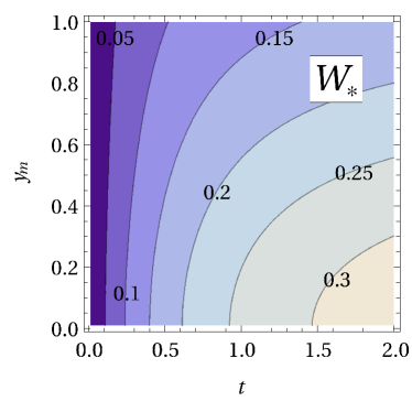
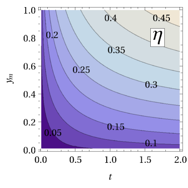
Figure 1: Performance of the machine with constant stiffness $k=1$ and optimally controlled center $\lambda(\tau)$. Extracted work $W_{*}$ and efficiency $\eta$ both as function of cycle time $t$ and measurement error $y_{m}$.

For a more powerful machine, we turn to a second variant where we allow additional control over the stiffness of the trap $k(\tau)$. In this case, the contribution (14) no longer vanishes. It becomes maximal for a standard deviation $y(\tau)$ increasing linearly from $y(0)=y_{i}^{+}$ to

$$y(t)=y_{i+1}^{-}=\frac{y_{i}^{+}+[(y_{i}^{+})^{2}+(2+t)t]^{1/2}}{2+t}.$$ (40)

In the stationary limit, $i\to\infty$, using (40) instead of (21) and the same reasoning to derive the limiting behavior as above, we obtain for the variance prior to a measurement in the steady state $(y_{*}^{-})^{2}$ the cubic equation

$$\left[(2+t)(y_{*}^{-})^{2}-t\right]^{2}[(y_{*}^{-})^{2}+y_{m}^{2}]-4(y_{*}^{-})^{4}y_{m}^{2}=0.$$ (41)

The limiting behavior of its solution is

$$(y_{*}^{-})^{2}\approx\left\{\begin{array}[]{l l}y_{m}t^{1/2}+(3/4-y_{m}^{2})t/2&{\rm~{}~{}~{}for~{}~{}~{}}t\to 0\\ {\displaystyle 1-\frac{2}{t}\left(1-\frac{y_{m}}{(1+y_{m}^{2})^{1/2}}\right)}&{\rm~{}~{}~{}for~{}~{}~{}}t\to\infty.\end{array}\right.$$ (44)

For (26) one obtains $(y_{*}^{+})^{2}$ with the short time and quasistatic behavior

$$(y_{*}^{+})^{2}\approx\left\{\begin{array}[]{l l}y_{m}t^{1/2}-(5/4+y_{m}^{2})t/2&{\rm for~{}}t\to 0\\ {\displaystyle\frac{y_{m}^{2}}{1+y_{m}^{2}}\left(1-\frac{2y_{m}^{2}(1+y_{m}^{2}-y_{m}(1+y_{m}^{2})^{1/2})}{(1+y_{m}^{2})^{2}t}\right)}&{\rm for~{}}t\to\infty.\end{array}\right.$$ (47)

For this second variant, we can still determine the contribution to the extracted work from (13) as in the first case, provided we use the solution of (41) in the expression (20) for the stationary limit. Collecting everything, we obtain for the extracted work the expression

$$W_{*}=-\frac{(y^{-}_{*})^{2}-(y_{*}^{+})^{2}}{4+t}-\frac{\left(y^{-}_{*}-y^{+}_{*}\right)^{2}}{t}+\ln(y^{-}_{*}/y^{+}_{*})$$ (48)

shown in Fig. 2. In this case, the power diverges in the short limit as

$$P\equiv\frac{W_{*}}{t}\approx\frac{1}{4y_{m}t^{1/2}}$$ (49)

whereas in the long time limit one obtains

$$P\approx\frac{1}{2t}\ln\left(1+\frac{1}{y_{m}^{2}}\right).$$ (50)

The short time divergence of the power is compensated by a corresponding divergence of the rate of information acquired through the measurements. Indeed, similarly as above, one gets the information per measurement

$${\cal I}_{*}\equiv\ln(y^{-}_{*}/y^{+}_{*})\approx\left\{\begin{array}[]{l l}t^{1/2}/(2y_{m})-(4+1/y_{m}^{2})t/16&{\rm for~{}}t\to 0\\ {\displaystyle\frac{1}{2}\ln\left(1+\frac{1}{y_{m}^{2}}\right)-\frac{1-y_{m}/(1+y_{m}^{2})^{\frac{1}{2}}}{t(1+y_{m}^{2})}}&{\rm for~{}}t\to\infty.\end{array}\right.$$ (53)

The efficiency of this machine becomes

$$\eta \equiv W_{*}/{\cal I}_{*}=1-\frac{\left((y^{-}_{*})^{2}-(y_{*}^{+})^{2}\right)/(4+t)+\left(y^{-}_{*}-y^{+}_{*}\right)^{2}/t}{\ln(y^{-}_{*}/y^{+}_{*})}$$ (54)

$$\approx \left\{\begin{array}[]{l l}1/2+t^{1/2}/(8y_{m})&{\rm~{}~{}~{}for~{}~{}~{}}t\to 0\\ 1-{\displaystyle\frac{4(1-y_{m}/(1+y_{m}^{2})^{1/2})}{t\ln(1+1/y_{m}^{2})}}&{\rm~{}~{}~{}for~{}~{}~{}}t\to\infty,\end{array}\right.$$ (57)

shown in Fig. 2.

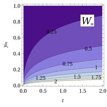
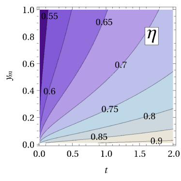
Figure 2: Performance of the machine with optimally controlled stiffness $k(\tau)$ and center $\lambda(\tau)$. Extracted work $W_{*}$ and efficiency $\eta$ both as function of cycle time $t$ and measurement error $y_{m}$.

For this variant, the efficiency increases with the cycle time starting at $\eta=1/2$ for $t\to 0$ and saturating the upper bound $\eta=1$ for $t\to\infty$ and any $y_{m}$. In this quasistatic case, in contrast to the first variant, the two control parameters allow to extract the full information. In another difference, the efficiency monotonically decreases with increasing $y_{m}$. Here, more precise measurements lead to a larger efficiency allowing even $\eta=1$ at finite $t$ for infinite precision $y_{m}\to 0$. In the full $(t,y_{m})$-plane, the efficiency is bounded by 1/2 from below. The value 1/2 found here in the short time limit that corresponds to maximum power may hint to a relation of our result with that for the efficiency of isothermal machines at maximum power where the value 1/2 is universal in the linear response regime [17]. While it is not obvious how to map repeated measurements for short cycle times to a linear response formalism, finding the same value in both cases may be more than incidental.

In conclusion, we have studied the efficiency for a cyclically operating Brownian information machine consisting of an overdamped particle in a time-dependent harmonic trap. For two variants of such a machine, we have obtained analytically how the efficiency depends on both the precision of a positional measurement and the cycle time. Beyond these specific results our work raises a few questions concerning such machines in general. First, while the quite natural definition of efficiency defined as mean extracted work divided by the mean acquired information shares features such as boundedness between 0 and 1 with the more conventional thermodynamic definition of efficiency for ordinary isothermal machines, finding $\eta=1$ even for finite cycle time in the limit of infinitely precise measurements, as we do for the second variant, suggests that these information machines differ in essential aspects from thermodynamics ones. For reaching $\eta=1$, the latter require a quasistatic operation, i.e., an infinite cycle time. Second, is it possible to formulate a linear response theory, i.e., to calculate Onsager coefficients for such machines? Third, can we derive general bounds on the efficiency at maximum power following reasoning for non-feedback driven machines? Finally, an experimental test of such a machine would be interesting and should be possible with available technology.

References

References

[1]
H. S. Leff and A. F. Rex.
Maxwell’s Demon : Entropy, Classical and Quantum Information,
Computing.
IOP, 2003.
[2]
H. Touchette and S. Lloyd.
Information-theoretic limits of control.
Phys. Rev. Lett., 84:1156, 2000.
[3]
R. Kawai, J. M. R. Parrondo, and C. van den Broeck.
Dissipation: The phase-space perspective.
Phys. Rev. Lett., 98:080602, 2007.
[4]
F. J. Cao and M. Feito.
Thermodynamics of feedback controlled systems.
Phys. Rev. E, 79:041118, 2009.
[5]
T. Sagawa and M. Ueda.
Generalized Jarzynski equality under nonequilibrium feedback
control.
Phys. Rev. Lett., 104:090602, 2010.
[6]
J. M. Horowitz and S. Vaikuntanathan.
Nonequilibrium detailed fluctuation theorem for repeated discrete
feedback.
Phys. Rev. E, 82:061120, 2010.
[7]
M. Esposito and C. van den Broeck.
Second law and Landauer principle far from equilibrium.
EPL, 95:40004, 2011.
[8]
D. Abreu and U. Seifert.
Thermodynamics of genuine non-equilibrium states under feedback
control.
Phys. Rev. Lett., 108:030601, 2012.
[9]
S. Lahiri, S. Rana, and A. M. Jayannavar.
Fluctuation theorems in the presence of information gain and
feedback.
J. Phys. A: Math. Theor., 45:065002, 2012.
[10]
T. Sagawa and M. Ueda.
Nonequilibrium thermodynamics of feedback control.
Phys. Rev. E, 85:021104, 2012.
[11]
S. Toyabe, T. Sagawa, M. Ueda, E. Muneyuki, and M. Sano.
Experimental demonstration of information-to-energy conversion and
validation of the generalized Jarzynski equality.
Nature Phys., 6:988, 2010.
[12]
A. Bérut, A. Arakelyan, A. Petrosyan, S. Ciliberto, R. Dillenschneider, and
E. Lutz.
Experimental verification of Landauer’s principle linking
information and thermodynamics.
Nature, 483:187, 2012.
[13]
R. Dillenschneider and E. Lutz.
Memory erasure in small systems.
Phys. Rev. Lett., 102:210601, 2009.
[14]
D. Abreu and U. Seifert.
Extracting work from a single heat bath through feedback.
Europhys. Lett., 94:10001, 2011.
[15]
J. M. Horowitz and J. M. R. Parrondo.
Designing optimal discrete-feedback thermodynamic engines.
New J. Phys., 13:123019, 2011.
[16]
T. Schmiedl and U. Seifert.
Efficiency at maximum power: An analytically solvable model for
stochastic heat engines.
EPL, 81:20003, 2008.
[17]
M. Esposito, K. Lindenberg, and C. van den Broeck.
Universality of efficiency at maximum power.
Phys. Rev. Lett., 102:130602, 2009.
[18]
Z. C. Tu.
Efficiency at maximum power of Feynman’s ratchet as a heat engine.
J. Phys. A: Math. Theor., 41:312003, 2008.
[19]
V. Blickle and C. Bechinger.
Realization of a micrometre-sized stochastic heat engine.
Nature Phys., 8:143, 2012.
[20]
U. Seifert.
Efficiency of autonomous soft nano-machines at maximum power.
Phys. Rev. Lett., 106:020601, 2011.