Quantum polarization tomography of bright squeezed light

Abstract

We reconstruct the polarization sector of a bright polarization squeezed beam starting from a complete set of Stokes measurements. Given the symmetry that underlies the polarization structure of quantum fields, we use the unique SU(2) Wigner distribution to represent states. In the limit of localized and bright states, the Wigner function can be approximated by an inverse three-dimensional Radon transform. We compare this direct reconstruction with the results of a maximum likelihood estimation, finding an excellent agreement.

1 Introduction

Polarization of light is a robust characteristic that can be efficiently manipulated using modest equipment without introducing more than marginal losses. It is thus not surprising that this is often the variable of choice to encode quantum information, as one can convince oneself by looking at some recent cutting-edge experiments, including quantum key distribution [1], quantum dense coding [2], quantum teleportation [3], rotationally invariant states [4], phase super-resolution [5], and weak measurements [6].

In the discrete-variable regime of single, or few, photons, one is mostly interested into two-mode states, which for all practical purposes can be regarded as a spin system [7, 8]. As a result, the polarization state can be determined from correlation functions of different orders [9, 10, 11, 12, 13, 14, 15, 16, 17, 18, 19]. Given the small dimensionality of the Hilbert space involved, the state reconstruction can be readily performed.

In the continuous-variable case, polarization properties are exploited for an expedient generation, manipulation, and measurement of nonclassical light. Polarization squeezing [20, 21, 22, 23], which has been observed in numerous experiments [24, 25, 26, 27, 28], is perhaps the most tantalizing illustration. Full Stokes polarimetry [29] is the method employed by the majority of the practitioners in this area.

However, the reconstruction in this limit is a touchy business and requires special care. The origin of the problem can be traced back to the fact that the characterization of the polarization state by the whole density operator is superfluous, because it contains much more than polarization information. This redundancy can easily be handled for low number of photons, but becomes a real hurdle for highly excited states. An adequate solution has been proposed recently: it suffices with a subset of the density matrix that has been called the “polarization sector” [30, 31] or the “polarization density operator” [32]. Its knowledge allows for a complete specification of the state on the Poincaré sphere (actually on a set of nested spheres that can be appropriately called the Poincaré space). The technique was devised by Karassiov and coworkers [33, 34, 35] and implemented experimentally in [36].

In this paper we present a comprehensive treatment of polarization tomography. As with any reliable quantum tomographical scheme, we need to supply three key ingredients [37]: the availability of a tomographically complete measurement, a suitable representation of the quantum states, and a robust algorithm for inverting the experimental data. In this respect, we use a standard Stokes scheme that implements the first ingredient in a very simple way; for the second, we resort to the well-known SU(2) Wigner distribution [38, 39, 40, 41, 42, 43, 44, 45], and finally, we prove that the inversion of the data in terms of that Wigner function is an inverse three-dimensional (3D) Radon transform.

To support the experimental feasibility of our scheme, we carry out the full tomography of a bright polarization-squeezed state generated in a Kerr medium [46]. The reconstruction is accomplished in three-different ways: by the direct inversion of the Radon transform, by a maximum-likelihood estimation and, finally, by a Gaussian approximation. The final results are compared and the sources of uncertainty are analyzed.

2 Setting the theoretical foundations

2.1 Polarization structure of quantum fields

A satisfactory description of the polarization structure of quantum fields and the corresponding observables that specify this structure is of paramount importance for our purposes.

We restrict our attention to the case of a monochromatic plane wave (the formalism can be easily extended to more involved multimode wavefronts [47, 48]), which we assume to propagate in the $z$ direction, so its electric field lies in the $xy$ plane. Under these conditions, we are dealing with a two-mode field that can be fully characterized by two complex amplitude operators. They are denoted by $\hat{a}_{H}$ and $\hat{a}_{V}$, where the subscripts $H$ and $V$ indicate horizontally and vertically polarized modes, respectively. The commutation relations of these operators are

$$[\hat{a}_{k},\hat{a}_{\ell}^{\dagger}]=\delta_{k\ell}\,,\qquad k,\ell\in\{H,V\}\,.$$ (2.1)

The description is greatly simplified if we use the Schwinger representation [49, 50]

$$\hat{J}_{1}=\textstyle\frac{1}{2}(\hat{a}^{\dagger}_{H}\hat{a}_{V}+\hat{a}^{\dagger}_{V}\hat{a}_{H})\,,\qquad\hat{J}_{2}=\frac{i}{2}(\hat{a}_{H}\hat{a}^{\dagger}_{V}-\hat{a}^{\dagger}_{H}\hat{a}_{V})\,,\qquad\hat{J}_{3}=\frac{1}{2}(\hat{a}^{\dagger}_{H}\hat{a}_{H}-\hat{a}^{\dagger}_{V}\hat{a}_{V})\,,$$ (2.2)

together with the total number

$$\hat{N}=\hat{a}^{\dagger}_{H}\hat{a}_{H}+\hat{a}^{\dagger}_{V}\hat{a}_{V}\,.$$ (2.3)

These operators coincide, up to a factor 1/2, with the Stokes operators [51], whose average values are precisely the classical Stokes parameters [52]. Using equation (2.1), one immediately notices that $\mathbf{\hat{J}}=(\hat{J}_{1},\hat{J}_{2},\hat{J}_{3})$ satisfy the commutation relations of the su(2) algebra

$$[\hat{J}_{k},\hat{J}_{\ell}]=i\epsilon_{k\ell m}\,\hat{J}_{m}\,,$$ (2.4)

where $\epsilon_{k\ell m}$ is the Levi-Civita fully antisymmetric tensor. This noncommutability precludes the simultaneous exact measurement of the physical quantities they represent. Among other consequences, this implies that no field state (apart from the vacuum) can have sharp nonfluctuating values of all the operators $\hat{\mathbf{J}}$ simultaneously. This is expressed by the uncertainty relation

$$\Delta^{2}\hat{\mathbf{J}}=\Delta^{2}\hat{J}_{1}+\Delta^{2}\hat{J}_{2}+\Delta^{2}\hat{J}_{3}\geq\langle\hat{N}\rangle/2\,,$$ (2.5)

where the variances are given by $\Delta^{2}\hat{J}_{i}=\langle\hat{J}_{i}^{2}\rangle-\langle\hat{J}_{i}\rangle^{2}$. In other words, the electric vector of a monochromatic quantum field never traces out a definite ellipse.

In classical optics, the total intensity is a well-defined quantity and the Poincaré sphere appears thus as a smooth surface with radius equal to that intensity. In quantum optics we have

$$\hat{J}_{1}^{2}+\hat{J}_{2}^{2}+\hat{J}_{3}^{2}=\left(\frac{\hat{N}}{2}\right)\left(\frac{\hat{N}}{2}+\leavevmode\hbox{\small 1\normalsize\kern-3.30002pt1}\right)\,,$$ (2.6)

and, as fluctuations in the number of photons are unavoidable (leaving aside photon-number states), we are forced to talk of a three-dimensional Poincaré space (with axis $J_{1}$, $J_{2}$ and $J_{3}$) that can be envisioned as foliated in a set of nested spheres with radii proportional to the different photon numbers that contribute significantly to the state.

The Hilbert space $\mathcal{H}$ of these two-mode fields has a convenient orthonormal basis in the form of Fock states for both polarization modes, namely $|n_{H},n_{V}\rangle$. However, since

$$[\hat{N},\hat{\mathbf{J}}]=0\,,$$ (2.7)

each subspace with a fixed number of photons $N$ must be handled separately. In other words, in the previous onion-like picture of the Poincaré space, each shell has to be addressed independently. This can be emphasized if instead of the Fock basis, we employ the relabeling

$$|J,m\rangle\equiv|n_{H}=J+m,n_{V}=J-m\rangle\,,$$ (2.8)

According to (2.6), we have that $J=N/2$ and this basis can be also seen as the common eigenstates of $\{\hat{J}^{2},\hat{J}_{3}\}$. In this way, for each fixed $J$ (i.e., fixed number of photons $N$), $m$ runs from $-J$ to $J$ and these states span a $(2J+1)$-dimensional subspace wherein $\hat{\mathbf{J}}$ acts in the usual way (in units $\hbar=1$)

$$\hat{J}_{\pm}|J,m\rangle=\sqrt{J(J+1)-m(m\pm 1)}|J,m\pm 1\rangle\,,$$

(2.9)

$$\hat{J}_{3}|J,m\rangle=m|J,m\rangle\,,$$

with $\hat{J}_{\pm}=\hat{J}_{1}\pm\hat{J}_{2}$.

It is clear from all this previous discussion that the moments of any energy-preserving observable (such as $\hat{\mathbf{J}}$) do not depend on the coherences between different subspaces. The only accessible information from any state described by the density matrix $\hat{\varrho}$ is thus its polarization sector, which is specified by the block-diagonal form

$$\hat{\varrho}_{\mathrm{pol}}=\bigoplus_{J}\hat{\varrho}^{(J)}$$ (2.10)

where $\hat{\varrho}^{(J)}$ is the reduced density matrix in the $J$ subspace. Any $\hat{\varrho}$ and its associated block-diagonal form $\hat{\varrho}_{\mathrm{pol}}$ cannot be distinguished in polarization measurements (and, accordingly, we drop henceforth the subscript pol). This is consistent with the fact that polarization and intensity are, in principle, independent concepts: in classical optics the form of the ellipse described by the electric field (polarization) does not depend on its size (intensity).

2.2 Polarization squeezing and the dark plane

The variances of the angular-momentum operators (2.2) are not independent, for they are constrained by

$$\Delta^{2}\hat{J}_{k}\,\Delta^{2}\hat{J}_{\ell}\geq\epsilon_{k\ell m}\,|\langle\hat{J}_{m}\rangle|^{2}\,.$$ (2.11)

It is always possible to find pairs of maximally conjugate operators for this uncertainty relation. This is equivalent to establishing a basis in which only one of the operators (2.2) has a nonzero expectation value, say $\langle\hat{J}_{k}\rangle=\langle\hat{J}_{\ell}\rangle=0$ and $\langle\hat{J}_{m}\rangle\neq 0$. The only nontrivial Heisenberg inequality reads thus

$$\Delta^{2}\hat{J}_{k}\,\Delta^{2}\hat{J}_{\ell}\geq|\langle\hat{J}_{m}\rangle|^{2}\,.$$ (2.12)

Polarization squeezing can then be sensibly defined as [20, 21, 22, 23]:

$$\Delta^{2}\hat{J}_{k}<|\langle\hat{J}_{m}\rangle|<\Delta^{2}\hat{J}_{\ell}\,.$$ (2.13)

The choice of the conjugate operators $\{\hat{J}_{k},\hat{J}_{\ell}\}$ is by not means unique: there exists an infinite set $\{\hat{J}_{\perp}(\theta),\hat{J}_{\perp}(\theta+\pi/2)\}$ that are perpendicular to the state classical excitation $\hat{J}_{m}$, for which $\langle\hat{J}_{\perp}(\theta)\rangle=0$ for all $\theta$. All these pairs exist in the $J_{k}$–$J_{\ell}$ plane, which is called the “dark plane” because it is the plane of zero mean intensity. We can express a generic $\hat{J}_{\perp}(\theta)$ as $\hat{J}_{\perp}(\theta)=\hat{J}_{k}\,\cos\theta+\hat{J}_{\ell}\,\sin\theta$, $\theta$ being an angle defined relative to $\hat{J}_{k}$. Condition (2.13) is then equivalent to

$$\Delta^{2}\hat{J}_{\perp}(\theta_{\mathrm{sq}})<\textstyle\frac{1}{2}|\langle\hat{N}\rangle|<\Delta^{2}\hat{J}_{\perp}(\theta_{\mathrm{sq}}+\pi/2),$$ (2.14)

where $\hat{J}_{\perp}(\theta_{\mathrm{sq}})$ is the squeezed parameter and $\hat{J}_{\perp}(\theta_{\mathrm{sq}}+\pi/2)$ the antisqueezed parameter.

In the experiments presented in this paper, a focal role will be played by the example in which the horizontal and vertical modes have the same amplitude but are phase shifted by $\pi/2$: $\langle\hat{a}_{H}\rangle=i\langle\hat{a}_{V}\rangle=i\alpha/\sqrt{2}$, $\alpha$ being a real number. This light is circularly polarized and fulfills $\langle\hat{J}_{1}\rangle=\langle\hat{J}_{3}\rangle=0$, $\langle\hat{J}_{2}\rangle=\alpha^{2}$. It is advantageous to work in the circular polarization basis, whose right $(+)$ and left $(-)$ amplitudes are given in terms of the linear ones by

$$\hat{a}_{\pm}=\frac{1}{\sqrt{2}}(\hat{a}_{H}\pm i\,\hat{a}_{V})\,.$$ (2.15)

In this manner, $\langle\hat{a}_{+}\rangle=\alpha$ and $\langle\hat{a}_{-}\rangle=0$. The operators in the $J_{1}$–$J_{3}$ plane correspond to the quadrature operators of the dark left-polarized mode. In fact, expressing the fluctuations of $\hat{\mathbf{J}}$ in terms of the noise of the circularly polarized modes $\delta\hat{a}_{\pm}$ and assuming $|\langle\delta\hat{a}_{\pm}\rangle|\ll\alpha$ we find [53]

$$\delta\hat{J}_{\perp}(\theta)=\alpha\delta\hat{X}_{-}(\theta)=\alpha[\delta\hat{X}_{H}(\theta)+\delta\hat{X}_{V}(\theta+\pi/2)]\,,$$ (2.16)

where $\hat{X}_{i}=(\hat{a}_{i}e^{-i\theta}+\hat{a}_{i}^{\dagger}e^{{i\theta}})/\sqrt{2}$ are the rotated quadratures for the $i$th amplitude. On the other hand, we have that

$$\delta\hat{N}=\alpha(\delta\hat{a}_{+}+\delta\hat{a}^{\dagger}_{+})=\alpha\,\delta\hat{X}_{+}\,,$$ (2.17)

and the intensity exhibits no dependence on the dark mode. In consequence, the condition (2.14) can be recast for this example as

$$\Delta^{2}\hat{J}_{\perp}(\theta)<|\langle\alpha\rangle|^{2}\quad\Leftrightarrow\quad\Delta^{2}\hat{X}_{-}(\theta)<1\,,$$ (2.18)

that is, polarization squeezing is equivalent to vacuum squeezing in the orthogonal polarization mode.

In the dark-plane measurements, the beam is divided equally between two photodetectors. Such measurements are then identical to balanced homodyne detection: the classical excitation is a local oscillator for the orthogonally polarized dark mode. The phase between these modes is varied by rotating the measurement through the dark plane, allowing a full characterization of the noise properties. This is a unique feature of polarization measurements and has been used in many experiments [54, 55, 56, 57, 58].

2.3 Polarization Wigner function

The structure discussed so far highlights that SU(2) is the symmetry group for polarization. To provide an appropriate phase-space description of states, we take advantage of the pioneering work of Stratonovich [38] and Berezin [39], who introduced quasi-probability distribution functions on the sphere satisfying all the proper requirements. This construction was later generalized by others [40, 41, 42, 43, 44, 45] and has proved to be very useful in visualizing properties of spinlike systems [59, 60, 61, 62, 63]

To gain physical insights into this approach, let us start by representing the density matrix with respect to the polarization basis. Instead of using directly the states $\{|J,m\rangle\}$, it is more convenient to write such an expansion as

$$\hat{\varrho}^{(J)}=\sum_{K=0}^{2J}\sum_{q=-K}^{K}\varrho_{Kq}^{(J)}\,\hat{T}_{Kq}^{(J)}\,,$$ (2.19)

where the irreducible tensor operators $T_{Kq}^{(J)}$ are [64]

$$\hat{T}_{Kq}^{(J)}=\sqrt{\frac{2K+1}{2J+1}}\sum_{m,m^{\prime}=-J}^{J}C_{Jm,Kq}^{Jm^{\prime}}\,|J,m^{\prime}\rangle\langle J,m|\,,$$ (2.20)

with $C_{Jm,Kq}^{Jm^{\prime}}$ being the Clebsch-Gordan coefficients that couple a spin $J$ and a spin $K$ ($0\leq K\leq 2J$) to a total spin $J$. These tensor operators have the right transformation properties under rotations and they indeed constitute the most suitable orthonormal basis

$$\Tr[\hat{T}_{Kq}^{(J)}\,\hat{T}_{K^{\prime}q^{\prime}}^{(J^{\prime})\,\dagger}]=\delta_{JJ^{\prime}}\delta_{KK^{\prime}}\delta_{qq^{\prime}}\,.$$ (2.21)

Although at first sight they might look a little bit intimidating, they are nothing but the multipoles used in atomic physics [65]: one can check that

$$\hat{T}_{00}^{(J)}=\frac{1}{\sqrt{2J+1}}\hat{\leavevmode\hbox{\small 1\normalsize\kern-3.30002pt1}}\,\qquad\hat{T}_{1q}^{(J)}=\sqrt{\frac{3}{(2J+1)(J+1)J}}\,\hat{J}_{q}\quad q=\pm,z\,,$$ (2.22)

and similarly the $\hat{T}^{(J)}_{Kq}$ can be related to the $K$th power of the generators (2.2). Accordingly, the expansion coefficients

$$\varrho_{Kq}^{(J)}=\Tr[\hat{\varrho}^{(J)}\,T_{Kq}^{(J)\,\dagger}]$$ (2.23)

are known as state multipoles.

The Wigner function associated with the state (2.19) is

$$W^{(J)}(\theta,\phi)=\Tr[\hat{\varrho}^{(J)}\,\hat{\Delta}^{(J)}(\theta,\phi)]\,,$$ (2.24)

where $\hat{\Delta}^{(J)}(\theta,\phi)$ is the Wigner kernel

$$\hat{\Delta}^{(J)}(\theta,\phi)=\sqrt{\frac{4\pi}{2J+1}}\sum_{K=0}^{2J}\sum_{q=-K}^{K}Y_{Kq}^{\ast}(\theta,\phi)\,\hat{T}_{Kq}^{(J)}\,,$$ (2.25)

and $Y_{Kq}(\theta,\phi)$ are the spherical harmonics. This kernel is unitary and satisfies the normalization conditions

$$\Tr[\hat{\Delta}^{(j)}(\theta,\phi)]=1\,,\qquad\frac{2J+1}{4\pi}\int_{\mathcal{S}^{2}}d\Omega\ \hat{\Delta}^{(j)}(\theta,\phi)=\hat{\leavevmode\hbox{\small 1\normalsize\kern-3.30002pt1}}\,.$$ (2.26)

The integral extends over the unit sphere $\mathcal{S}^{2}$ and $d\Omega$ is the invariant measure therein, namely, $d\Omega=\sin\theta\,d\theta d\phi$.

From (2.24) and the properties of the irreducible tensors, one can immediately express the Wigner function in the very suggestive form

$$W^{(J)}(\theta,\phi)=\sum_{K=0}^{2J}\sum_{q=-K}^{K}\varrho_{Kq}^{(J)}\;Y_{Kq}^{\ast}(\theta,\phi)\,,$$ (2.27)

which clearly shows that determining this Wigner function is tantamount to the knowledge of all the state multipoles. (i.e., all the moments of the Stokes parameters).

One can obtain the marginal of $W^{(J)}(\theta,\phi)$ once summed over all the values of $J$

$$W(\theta,\phi)=\sum_{J}\frac{2J+1}{4\pi}W^{(J)}(\vartheta,\varphi)\,,$$ (2.28)

where the factor has been introduced to ensure the proper normalization.

In the above-mentioned example of a strong circularly polarized state, we can consider that the sphere can locally be replaced by its tangent plane since $J\simeq\alpha^{2}$. Using simple geometrical relations between the coordinates $(\theta,\phi)$ and the Cartesian coordinates $(q,p)$ in that tangent plane, we get

$$W(\theta,\phi)\simeq\alpha\;W(q,p)\,,$$ (2.29)

which confirms that the dark plane is equivalent to the standard phase space for continuous variables.

In the limit of large photon numbers the representation (2.24) is not very useful. In such a case, a remarkably effective approximation is given by[66]

$$\hat{\Delta}^{(J)}(\theta,\phi)\simeq(-1)^{J}\exp(-i\pi\mathbf{n}\cdot\hat{\mathbf{J}})\,,$$

where $\mathbf{n}=(\cos\theta\sin\phi,\sin\theta\sin\phi,\cos\theta)$ is the unitary vector in the direction $(\theta,\phi)$.

2.4 Tomograms and tomographic inversion

A general polarimetric apparatus consists of a half-wave plate, with axis at angle $\alpha$, followed by a quarter-wave plate at angle $\beta$. For fixed values of the angles $(\alpha,\beta)$ of the wave plates, the selected direction in the Stokes space is

$$\theta=\pi/2-2\beta\,,\qquad\phi=2\beta-4\alpha\,.$$ (2.30)

The polarization transformations performed by the wave plates can be represented by $\hat{J}_{2}$, which generates rotations about the direction of propagation, and $\hat{J}_{3}$, which generates phase shifts between the modes. Their joint action is given by the operator

$$\hat{D}(\theta,\phi)=e^{i\theta\hat{J}_{2}}\,e^{i\phi\hat{J}_{3}}\,,$$ (2.31)

which describes displacements over the sphere. After that, a polarizing beam splitter projects onto the basis $|J,m\rangle$.

In physical terms, the wave plates transform the input polarization allowing the measurement of different Stokes parameters by the projection onto the basis $|J,m\rangle$. This can be modeled by

$$\hat{\Pi}_{m}^{(J)}=|J,m\rangle\langle J,m|\,,$$ (2.32)

so that $w_{m}^{(J)}=\Tr[\hat{\varrho}\hat{\Pi}_{m}^{(J)}]$ is the probability of detecting $n_{H}=J+m$ photons in the horizontal mode and simultaneously $n_{V}=J-m$ photons in the vertical one. Of course, when the total number of photons is not measured and only the difference $m$ is observed, it reduces to

$$\Pi_{m}=\sum_{J=|m|}^{\infty}|J,m\rangle\langle J,m|\,.$$ (2.33)

The experimental histograms recorded for each direction $(\theta,\phi)$ correspond to the tomographic probabilities

$$w^{(J)}_{m}(\theta,\phi)=\Tr[\hat{\varrho}\,\hat{\Pi}_{m}^{(J)}(\theta,\phi)]=\Tr[\hat{\varrho}\,\hat{D}(\theta,\phi)\,\hat{\Pi}_{m}^{(J)}\,\hat{D}^{\dagger}(\theta,\phi)]\,.$$ (2.34)

The reconstruction in each $(2J+1)$-dimensional invariant subspace can now be carried out exactly since it is essentially equivalent to a spin $J$ [67, 68, 69, 70]. One can proceed in a variety of ways, but perhaps the simplest one is to look for an integral representation of the tomograms (2.34); as soon as one realizes that

$$\hat{\Pi}_{m}^{(J)}(\theta,\phi)=\frac{1}{2\pi}\int_{0}^{2\pi}d\omega\,\exp[i\omega(\hat{\mathbf{J}}\cdot\mathbf{n}-m)]\,,$$ (2.35)

the tomograms read as

$$w_{m}^{(J)}(\theta,\phi)=\frac{1}{2\pi}\int_{0}^{2\pi}d\omega\,\Tr[\hat{\varrho}^{(J)}\,\exp(i\omega\hat{\mathbf{J}}\cdot\mathbf{n})]\,e^{-i\omega m}\,,$$ (2.36)

that is, they appear as the Fourier transform of the characteristic function for the observable $\hat{\mathbf{J}}\cdot\mathbf{n}$. After some direct manipulations, we find that

$$\hat{\varrho}^{(J)}=\frac{1}{4\pi}\sum_{m=-J}^{J}\int_{\mathcal{S}_{2}}d\mathbf{n}^{\prime}\ w_{m}^{(J)}(\mathbf{n}^{\prime})\,\mathcal{K}(\hat{\mathbf{J}}\cdot\mathbf{n}^{\prime}-m)\,,$$ (2.37)

where $d\mathbf{n}^{\prime}$ indicates integration over the unit sphere and the kernel $\mathcal{K}(x)$ is

$$\mathcal{K}(x)=\frac{2J+1}{4\pi^{2}}\int_{0}^{2\pi}d\omega\;\sin^{2}\left(\frac{\omega}{2}\right)\,e^{-i\omega x}\,.$$ (2.38)

Although (2.37) is a formal solution, it is handier to map this density matrix onto the corresponding Wigner function, for which we need to compute $\Tr[\mathcal{K}(\mathbf{J}\cdot\mathbf{n}^{\prime}-m)\,\hat{\Delta}^{(J)}(\theta,\phi)]$. When $J$ is large enough, we can replace the Wigner kernel by its approximate expression (2.3), getting

$$\Tr[\mathcal{K}(\mathbf{J}\cdot\mathbf{n}^{\prime}-m)\,\hat{\Delta}^{(J)}(\theta,\phi)]=(-1)^{J}\frac{2J+1}{4\pi^{2}}\int_{0}^{2\pi}d\omega\,\sin^{2}\left(\frac{\omega}{2}\right)e^{-im\omega}\chi_{J}(\omega^{\prime})\,,$$ (2.39)

where $\chi_{J}(\omega^{\prime})$ is the character of the $(2J+1)$-dimensional representation of the SU(2) group [64] and $\omega^{\prime}$ is given by

$$\cos\left(\frac{\omega^{\prime}}{2}\right)=\mathbf{n}\cdot\mathbf{n}^{\prime}\,\sin\left(\frac{\omega}{2}\right)\,.$$ (2.40)

For $J\gg~{}1$, $m$ can be taken as a continuous variable. Replacing the sum by an integral, integrating by parts and taking into account that for localized states $\mathbf{n}\cdot\mathbf{n}^{\prime}\simeq 1$, the Wigner function simplifies to

$$W(J,\theta,\phi)=\frac{2J+1}{4\pi^{2}}\int_{-\infty}^{\infty}\!dm\int_{\mathcal{S}_{2}}\!d\mathbf{n}^{\prime}\,\frac{d^{2}w_{m}^{(J)}(\mathbf{n})}{dm^{2}}\,\delta(m-J\,\mathbf{n}\cdot\mathbf{n}^{\prime})\,,$$ (2.41)

where we have included $J$ as an argument to stress that it must be treated as continuous. The reconstruction in this limit turns out to be equivalent to an inverse Radon transform of the measured tomograms.

3 Experiment

3.1 The setup

To validate our approach, we perform the tomography of a polarization squeezed state, generated in a polarization-maintaining optical fibre through the nonlinear Kerr effect [46]. The setup is shown in figure 1. The light source is a shot-noise limited ORIGAMI laser from Onefive GmbH emitting 220 fs pulses at a repetition rate of 80 MHz and centered at 1560 nm. The light is fed into a 13 m-long polarization-maintaining birefringent fibre (3M FS-PM-7811, 5.6 $\mu$m mode-field diameter) so that quadrature squeezed states are simultaneously and independently generated in both polarization modes. The strong birefringence of the fibre (beat length 1.67 mm) causes a delay between the emerging quadrature-squeezed pulses. We precompensate for this delay in an unbalanced Michelson-like interferometer placed before the fibre. A small part (0.1 %) of the fibre output serves as the input to a control loop to maintain the relative phase between the exiting pulses locked to $\pi/2$, so the light is circularly polarized.

Figure 1: Setup for efficient polarization squeezing generation and the corresponding Stokes measurement apparatus.

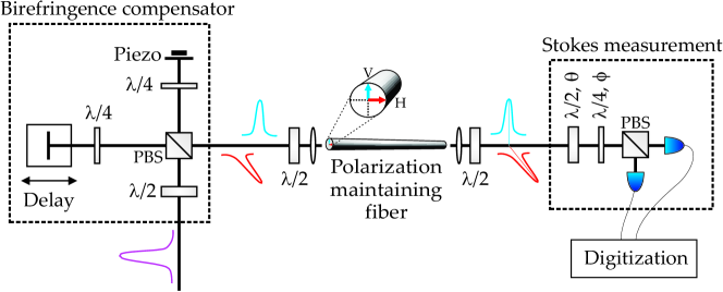
The quantum state is detected with a Stokes measurement, as sketched in the previous section. The two detectors (InGaAS PIN photodiodes, custom-made by Laser Components GmbH with 98 % quantum efficiency at DC) are balanced and have a sub-shot noise resolution at a frequency range between 5 MHz and 30 MHz. Each detector has two separate outputs: DC, providing the average values of the photocurrents, and AC, providing the photocurrents amplified in radio-frequency (RF) spectral range. The RF currents of the photodetectors are mixed with an electronic local oscillator at 12 MHz, amplified (FEMTO DHPVA-100), and digitized by an analog/digital exit converter (Gage CompuScope 1610) at 10 Megasamples per second with a 16-bit resolution and 10 times oversampling.

The measurements are performed at a pulse energy of 93 pJ. In the dark plane a total squeezing of about 3.8 dB is observed. In the orthogonal quadrature, the noise was enhanced by several tens of dB due to Guided Acoustic Wave Brillouin Scattering (GAWBS) [71, 72, 73]. In the direction of the classical excitation, the state is expected to be shot-noise limited, since the Kerr effect only influences the phase and does not contribute to the photon number.

To perform the reconstruction, histograms of the Stokes variables are recorded for different angles $(\theta,\phi)$. This is done by rotating the wave plates with motorized stages (OWIS DMT 40-D20-HSM) and scanning one eighth of the Poincaré sphere in 8100 steps, a measurement that took over eight hours. The unmeasured octants were deduced from symmetry. For each setting of the wave plates, the photocurrent noise of both detectors was simultaneously sampled $0.5\times 10^{6}$ times. Noise statistics of the detectors difference current were acquired in histograms with 751 bins. Additionally, the optical intensity was recorded.

In figure 2 we show typical histograms at different angles on the Poincaré sphere. As the widths largely vary from squeezing to antisqueezing ranges, there are two plots in which the amplitude scale differs in more than one order of magnitude. The histograms labeled 1, 2 and 3 are measured in the dark plane. Tomogram 1 denotes the angle of maximum squeezing, while 3 corresponds to the antisqueezing. Tomogram 4 is at the classical mean value, where the measured noise is almost shot-noise limited. Due to the high number of samples, the measured histograms are smooth and, at the same time, the number of bins makes it possible to resolve the large dynamical range of amplitudes, so no data interpolation was needed. We also plot histograms showing the electronic noise and the shot noise.

Figure 2: Measured histograms of the difference current of the two detectors for various measurement directions on the Poincaré sphere.. Note the different scales on both plots. Histograms 1, 2, and 3 are in the dark plane, while histogram 4 is at the classical mean value. The histograms corresponding to electronic and shot noise are also shown.

For all these histograms we have performed a Gaussianity check, using the Kolmogorov-Smirnov and the $\chi^{2}$ tests, as well as the Kullback-Leibler divergence[74]. We can conclude that all the histogramas are Gaussian within confidence levels ranging from 95 % to 98 %.

3.2 Experimental reconstruction

As clearly expressed in (2.41), for high photon numbers the tomography turns out to be equivalent to an inverse Radon transform of the measured histograms. In practice, this one-step 3D reconstruction is very demanding in computational resources. Therefore, we divide the process into two steps: first, a set of 2D projections is reconstructed from the recorded histograms; subsequently, the Wigner function is slice-wise generated from those projections (to which we apply a Hamming filter to smooth the noise). The symmetry of the state is used as a prior information to reduce the range of measured angles to an octant. This minimizes the systematic errors stemming from imperfections of the polarization optics.

Figure 3: (Right) Isocontour surface of the level $1/e$ (from the maximum) of the Wigner function $W(J,\theta,\phi)$ for the polarization squeezed state generated in the setup of figure 1. (Left) Sections of the Wigner function through the three coordinate planes. In blue we show the isotropic section for a coherent state, which we use as unit for all the plots.

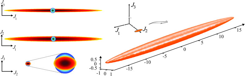
In figure 3 (right panel) we show the final result of the inverse Radon transform for our polarization squeezed state. More concretely, we plot an isocontour surface of $W(J,\theta,\phi)=\,$ constant (with the constant being $1/e$ from the maximum) in the Poincaré space having $J_{1}$, $J_{2}$, and $J_{3}$ as orthogonal axes. As coordinate units we use the shot noise set by a coherent state. The ellipsoidal shape of the state is clearly visible. The center of the ellipsoid is far away from the origin, since we have $10\times 10^{11}$ photons per measurement time (using 1.9 MHz resolution bandwidth). The antisqueezed direction of the ellipsoid is dominated by excess noise stemming largely from GAWBS, as we have already mentioned.

In the left panel of figure 3 we sketch density plots of the projections on the coordinate planes of the previous Wigner function (including the particular case of a coherent state). The contours agree with the 3.8 $\pm$ 0.3 dB squeezing that was directly measured from the variances. The projections on the planes $J_{1}$-$J_{2}$ and $J_{2}$-$J_{3}$ show an additional spreading of the state in the $J_{2}$ direction caused by the imperfect polarization contrast in the measurement setup that mixes some of the antisqueezing on the $J_{2}$ direction.

This Radon reconstruction requires a large set of measured data to get a reasonably accurate representation of the state. There are two main reasons for this: integrals are approximated by finite sums (in our case, we used 751 bins in 91 steps) and the kernel (2.38) is singular, so some ad hoc filtering of the raw data is needed. Acquiring such large data sets may be unwise, for it demands long measurement times. Ensuring the proper stability of the setup is thus essential and might be difficult depending on the quantum state measured.

This limitation may be circumvented by adopting a statistically-motivated method, such as the maximum likelihood (ML) [75]. In our case, the relation between the Wigner function $W$ and the tomograms $w$ can be written as a system of linear equations

$$w_{j}=\sum_{j}c_{jk}\,W_{k},$$ (3.1)

where the subscripts in $W_{k}$ and $w_{j}$ is a shorthand notation for the respectives coordinates. The coefficients $c_{jk}$ can be interpreted as the overlap of the $j$th projector with the $k$th volume element of the Wigner function and can be readily determined from equations (2.27) and (2.34). The most likely Wigner function is then found by minimizing the Kullback-Leibler divergence between the normalized vectors of the computed tomograms $w_{j}$ and recorded ones $\bar{w}_{j}$. Technically, this can be achieved by the iterative expectation-maximization algorithm [76, 77, 78]

$$W_{k}^{(n+1)}=W_{k}^{(n)}\frac{\sum_{j}w_{j}}{(\sum_{j}\bar{w}_{j})(\sum_{j}c_{jk})}\sum_{j}\frac{\bar{w}_{j}}{w_{j}}c_{jk}\,,$$ (3.2)

which converges monotonously to the ML estimate from any strictly positive initial vector $W_{k}^{(0)}$.

Figure 4: Sections of the isocontour of the Wigner function in figure 3 through the coordinate axes, for the three different reconstruction techniques used. In grey, direct Radon transform, in green ML method with nine settings for the angles of the wave plates and in dotted lines the results of a Gaussian ML approximation.

The significantly greater stability of the statistical inversion allows us to get reconstructions of the same quality but from far smaller data sets. This is illustrated in figure 4, where we draw a comparison between Radon and ML methods, although in the latter case using only nine different settings of the angles $(\theta,\phi)$, which amounts to reducing the measurements by two orders of magnitude. In other words, the measuring time is shortened from eight hours to less than five minutes! This result indicates that the experimental characterization of considerably more complicated quantum states with less symmetries should still be within the reach of the present measurement setup.

As we have discussed in section 2.2, the dark plane is of special interest. The theory shows that the reconstruction therein can be obtained in two different ways: either by reconstructing the dark mode directly from the histograms or by calculating projection of the 3D Wigner function along the $J_{2}$ direction. The two results are compared in figure 5 and good agreement within the experimental uncertainties is found. Since the Radon transform should provide a plausible explanation for all the measured histograms, such a comparison may serve as an independent test of the quality of the 3D tomography.

Figure 5: Dark plane reconstructions. Left panel: Reconstruction obtained by integrating the Wigner function shown in figure. 3 in the $J_{2}$ direction. Right panel: ML reconstruction from dark-plane histograms. Only nine settings of angles $\theta$ and $\phi$ were used for the ML tomography.

Finally, the high confidence levels of the Gaussianity tests seems to call for a Gaussian ML reconstruction. The Gaussianity is used as a prior information about the signal, which helps to reduce drastically the number of free parameters. In this case, the Wigner function is represented by the $3\times 3$ covariance matrix $G$:

$$W(\mathbf{n})\propto\exp\left(-\frac{1}{2}\mathbf{n}G^{-1}\mathbf{n}\right)\,,$$ (3.3)

and the calculated variances $\sigma_{j}=\mathbf{n}_{j}G\mathbf{n}_{j}$ are matched (in the ML sense) to the actually measured variances [79]. Since $G$ must be positive semidefinite, only six real parameters describe the measured system and the problem is highly overdetermined, in consequence, the Gaussian state can be obtained from a few histograms. In principle, by comparing Gaussian reconstructions based on different subsets of measured data, various imperfections of the setup, such as instabilities and biases, can be detected.

The matrix $G$ turns out to be

$$G=\left(\begin{array}[]{ccc}3.0920\times 10^{2}&-1.1931&-2.0160\\ -1.1931&4.4485\times 10^{-1}&-1.2926\times 10^{-2}\\ -2.0160&-1.2926\times 10^{-2}&1.1511\end{array}\right)\,,$$ (3.4)

which once diagonalized gives the principal variances 0.43962, 1.13853, and 309.22177 (in shot-noise units). This agrees well with the standard and ML reconstructions, as can be also appreciated in figure 4. The Gaussian reconstruction was done without assuming a particular orientation or symmetry of the state with respect to the Stokes coordinates. The covariance matrix suggests that the misalignment of the principal axis is less than $0.5$ degrees within the measurement errors, in accordance with the definition of angles adopted in the experiment.

This Gaussian approach allows for a simple estimate of the errors: just take the pseudoinversion of the measurement matrix as a linear model and use the standard theory of error propagation. The errors to be propagated are actually the errors in the estimated variances for each tomogram, which are found from the $\chi^{2}$ distribution. In addition, we can assume that the variances of different tomograms are uncorrelated.

Taking a 97.5 % confidence interval (which corresponds to three standard deviations), the principal variances can be written as

$$0.440\pm 0.002,\quad 1.139\pm 0.001,\quad 309.2\pm 0.3\,.$$ (3.5)

Note that the relative errors in the two larger variances are roughly the same ($\sim$ 0.1 %), while for the smallest variance is four times larger. This is a consequence of the experimental setup: the smallest variance is directly revealed only in one of the recorded projections used for the reconstruction.

4 Concluding remarks

In summary, we have presented a complete programme for the full polarization tomography of quantum states. Using the SU(2) Wigner function, we have provided an exact inversion formula in terms of the histograms of a standard Stokes measurement and derived a simplified version for very localized, high intensity states which turns out to be an inverse Radon transform. As a test of the theory, the reconstruction of an intense polarization squeezed state has been performed. A ML reconstruction algorithm has also been presented and has been compared to the direct method, thereby yielding an excellent agreement. Of course, the technique can be readily used for any other polarization state.

References

- [1] Muller A, Breguet J and Gisin N 1993 Europhys. Lett. 23 383–388
- [2] Mattle K, Weinfurter H, Kwiat P G and Zeilinger A 1996 Phys. Rev. Lett. 76 4656–4659
- [3] Bouwmeester D, Pan J W, Mattle K, Eibl M, Weinfurter H and Zeilinger A 1997 Nature 390 575–579
- [4] Rådmark M, Żukowski M and Bourennane M 2009 New J. Phys. 11 103016
- [5] Resch K J, Pregnell K L, Prevedel R, Gilchrist A, Pryde G J, O’Brien J L and White A G 2007 Phys. Rev. Lett. 98 223601
- [6] Dixon P B, Starling D J, Jordan A N and Howell J C 2009 Phys. Rev. Lett. 102 173601
- [7] Lamas-Linares A, Howell J C and Bouwmeester D 2001 Nature 412 887–890
- [8] Sehat A, Söderholm J, Björk G, Espinoza P, Klimov A B and Sánchez-Soto L L 2005 Phys. Rev. A 71 033818
- [9] White A G, James D F V, Eberhard P H and Kwiat P G 1999 Phys. Rev. Lett. 83 3103–3107
- [10] Kwiat P G, Berglund A J, Altepeter J B and White A G 2000 Science 290 498–501
- [11] James D F V, Kwiat P G, Munro W J and White A G 2001 Phys. Rev. A 64 052312
- [12] Thew R T, Nemoto K, White A G and Munro W J 2002 Phys. Rev. A 66 012303
- [13] Barbieri M, De Martini F, Di Nepi G, Mataloni P, D’Ariano G M and Macchiavello C 2003 Phys. Rev. Lett. 91 227901
- [14] Bogdanov Y I, Chekhova M V, Kulik S P, Maslennikov G A, Zhukov A A, Oh C H and Tey M K 2004 Phys. Rev. Lett. 93 230503
- [15] Moreva E V, Maslennikov G A, Straupe S S and Kulik S P 2006 Phys. Rev. Lett. 97 023602
- [16] Barbieri M, Vallone G, Mataloni P and De Martini F 2007 Phys. Rev. A 75 042317
- [17] Adamson R B A and Steinberg A M 2010 Phys. Rev. Lett. 105 030406
- [18] Sansoni L, Sciarrino F, Vallone G, Mataloni P, Crespi A, Ramponi R and Osellame R 2010 Phys. Rev. Lett. 105 200503
- [19] Altepeter J B, Oza N N, Medi M, Jeffrey E R and Kumar P 2011 Opt. Express 19 26011–26016
- [20] Chirkin A S, Orlov A A and Parashchuk D Y 1993 Quantum Electron. 23 870–874
- [21] Korolkova N, Leuchs G, Loudon R, Ralph T C and Silberhorn C 2002 Phys. Rev. A 65 052306
- [22] Luis A and Korolkova N 2006 Phys. Rev. A 74 043817
- [23] Mahler D, Joanis P, Vilim R and de Guise H 2010 New J. Phys. 12 033037
- [24] Bowen W P, Schnabel R, Bachor H A and Lam P K 2002 Phys. Rev. Lett. 88 093601
- [25] Heersink J, Gaber T, Lorenz S, Glöckl O, Korolkova N and Leuchs G 2003 Phys. Rev. A 68 013815
- [26] Dong R, Heersink J, Yoshikawa J I, Glöckl O, Andersen U L and Leuchs G 2007 New J. Phys. 9 410
- [27] Shalm L K, A A R B and Steinberg A M 2009 Nature 457 67–70
- [28] Iskhakov T, Chekhova M V and Leuchs G 2009 Phys. Rev. Lett. 102 183602
- [29] Brosseau C 1998 Fundamentals of Polarized Light: A Statistical Optics Approach (New York: Wiley)
- [30] Raymer M G and Funk A C 1999 Phys. Rev. A 61 015801
- [31] Raymer M G, McAlister D F and Funk A 2000 Measuring the quantum polarization state of light Quantum Communication, Computing, and Measurement 2 ed Kumar P (New York: Plenum)
- [32] Karassiov V P 1993 J. Phys. A 26 4345–4354
- [33] Bushev P A, Karassiov V P, Masalov A V and Putilin A A 2001 Opt. Spectrosc. 91 526–531
- [34] Karassiov V P and Masalov A V 2004 JETP 99 51–60
- [35] Karassiov V 2005 J. Russ. Las. Res. 26 484–513
- [36] Marquardt C, Heersink J, Dong R, Chekhova M V, Klimov A B, Sánchez-Soto L L, Andersen U L and Leuchs G 2007 Phys. Rev. Lett. 99 220401
- [37] Hradil Z, Mogilevtsev D and Řeháček J 2006 Phys. Rev. Lett. 96 230401
- [38] Stratonovich R L 1956 JETP 31 1012—1020
- [39] Berezin F A 1975 Commun. Math. Phys. 40 153–174
- [40] Agarwal G S 1981 Phys. Rev. A 24 2889–2896
- [41] Brif C and Mann A 1998 J. Phys. A 31 L9–L17
- [42] Varilly J C and Gracia-Bondía J M 1989 Ann. Phys. 190 107–148
- [43] Heiss S and Weigert S 2000 Phys. Rev. A 63 012105
- [44] Klimov A B and Chumakov S M 2000 J. Opt. Soc. Am. A 17 2315–2318
- [45] Klimov A B and Romero J L 2008 J. Phys. A 41 055303
- [46] Heersink J, Josse V, Leuchs G and Andersen U L 2005 Opt. Lett. 30 1192–1194
- [47] Karassiov V P 2006 JETP Lett. 84 640–644
- [48] Karassiov V P and Kulik S P 2007 JETP 104 30—46
- [49] Schwinger J 1965 On angular momentum Quantum Theory of Angular Momentum ed Biedenharn L C and Dam H (New York: Academic)
- [50] Chaturvedi S, Marmo G and Mukunda N 2006 Rev. Math. Phys. 18 887–912
- [51] Luis A and Sánchez-Soto L L 2000 Prog. Opt. 41 421–481
- [52] Born M and Wolf E 1999 Principles of Optics 7th ed (Cambridge: Cambridge University Press)
- [53] Corney J F, Heersink J, Dong R, Josse V, Drummond P D, Leuchs G and Andersen U L 2008 Phys. Rev. A 78 023831
- [54] Grangier P, Slusher R E, Yurke B and LaPorta A 1987 Phys. Rev. Lett. 59 2153–2156
- [55] Smithey D T, Beck M, Raymer M G and Faridani A 1993 Phys. Rev. Lett. 70 1244–1247
- [56] Schnabel R, Bowen W P, Treps N, Ralph T C, Bachor H A and Lam P K 2003 Phys. Rev. A 67 012316
- [57] Julsgaard B, Sherson J, Cirac J I, Fiurasek J and Polzik E S 2004 Nature 432 482–486
- [58] Josse V, Dantan A, Bramati A and Giacobino E 2004 J. Opt. B 6 S532–S543
- [59] Dowling J P, Agarwal G S and Schleich W P 1994 Phys. Rev. A 49 4101–4109
- [60] Atakishiyev N M, Chumakov S M and Wolf K B 1998 J. Math. Phys. 39 6247–6261
- [61] Chumakov S M, Frank A and Wolf K B 1999 Phys. Rev. A 60 1817–1822
- [62] Chumakov S M, Klimov A B and Wolf K B 2000 Phys. Rev. A 61 034101
- [63] Klimov A B 2002 J. Math. Phys. 43 2202–2213
- [64] Varshalovich D A, Moskalev A N and Khersonskii V K 1988 Quantum Theory of Angular Momentum (Singapore: World Scientific)
- [65] Blum K 1981 Density Matrix Theory and Applications (New York: Plenum)
- [66] Klimov A B and Chumakov S M 2000 J. Opt. Soc. Am. A 17 2315–2318
- [67] Brif C and Mann A 1999 Phys. Rev. A 59 971–987
- [68] Amiet J P and Weigert S 1999 J. Phys. A 32 L269–L274
- [69] D’Ariano G M, Maccone L and Paini M 2003 J. Opt. B 5 77–84
- [70] Klimov A B, Man’ko O V, Man’ko V I, Smirnov Y F and Tolstoy V N 2002 J. Phys. A 35 6101–6123
- [71] Shelby R M, Levenson M D and Bayer P W 1985 Phys. Rev. B 31 5244–5252
- [72] Shelby R M, Levenson M D, Perlmutter S H, DeVoe R G and Walls D F 1986 Phys. Rev. Lett. 57 691–694
- [73] Elser D, Andersen U L, Korn A, Glöckl O, Lorenz S, Marquardt C and Leuchs G 2006 Phys. Rev. Lett. 97 133901
- [74] Thode H C 2002 Testing for Normality (New York: Marcel Dekker)
- [75] Paris M G A and Řeháček J (eds) 2004 Quantum State Estimation (Lect. Not. Phys. vol 649) (Berlin: Springer)
- [76] Dempster A P, Laird N M and Rubin D B 1977 J. R. Statist. Soc. B 39 1–38
- [77] Boyles R A 1983 J. R. Statist. Soc. B 45 47–50
- [78] Vardi Y and Lee D 1993 J. R. Statist. Soc. B 55 569–612
- [79] Řeháček J, Olivares S, Mogilevtsev D, Hradil Z, Paris M G A, Fornaro S, D’Auria V, Porzio A and Solimeno S 2009 Phys. Rev. A 79 032111