Mean-field analysis of the majority-vote model broken-ergodicity steady state

Abstract

We study analytically a variant of the one-dimensional majority-vote model in which the individual retains its opinion in case there is a tie among the neighbors’ opinions. The individuals are fixed in the sites of a ring of size $L$ and can interact with their nearest neighbors only. The interesting feature of this model is that it exhibits an infinity of spatially heterogeneous absorbing configurations for $L\to\infty$ whose statistical properties we probe analytically using a mean-field framework based on the decomposition of the $L$-site joint probability distribution into the $n$-contiguous-site joint distributions, the so-called $n$-site approximation. To describe the broken-ergodicity steady state of the model we solve analytically the mean-field dynamic equations for arbitrary time $t$ in the cases $n=3$ and $4$. The asymptotic limit $t\to\infty$ reveals the mapping between the statistical properties of the random initial configurations and those of the final absorbing configurations. For the pair approximation ($n=2$) we derive that mapping using a trick that avoids solving the full dynamics. Most remarkably, we find that the predictions of the $4$-site approximation reduce to those of the $3$-site in the case of expectations involving three contiguous sites. In addition, those expectations fit the simulation data perfectly and so we conjecture that they are in fact the exact expectations for the one-dimensional majority-vote model.

1 Introduction

A desirable property of a model for social behavior, or for complex systems in general, is the presence of a nontrivial steady state characterized by infinitely many equilibrium points in the thermodynamic limit. This was the main appeal of the mean-field spin-glass models used widely since the 1980s to study associative memory [1], prebiotic evolution [2], ecosystem organization [3], and social systems [4] to name just a few of the areas impacted by the spin-glass approach to model complex systems [5].

Models of social dynamics, however, are typically defined through the specification of the dynamic rules that govern the interactions between agents [6] and so they are not amenable to analysis using tools borrowed from the equilibrium statistical mechanics of disordered systems. Nevertheless, the display of a steady state characterized by a multitude of locally stable and spatially inhomogeneous configurations remains a celebrated feature of this class of models, whose paradigm is Axelrod’s model [7], since they can explain the diversity of cultures or opinions observed in human societies. Axelrod’s model is attractive from the statistical physics perspective because it exhibits a nonequilibrium phase transition which separates the spatially homogeneous (mono-cultural) from the heterogeneous (multicultural) regimes [8, 9, 10].

More recently, a long-familiar model of lattice statistical physics – the majority-vote model [11, 12] – was revisited in the context of social dynamics models [13, 14]. In fact, the majority-vote model is a lattice version of the classic frequency bias mechanism for opinion change [19], which assumes that the number of people holding an opinion is the key factor for an agent to adopt that opinion, i.e., people have a tendency to espouse opinions that are more common in their social environment. The variant of the majority-vote model considered in those studies includes the state of the target site (the voter) in the reckon of the majority (hence we refer to the model as extended majority-vote model), which happens to be the variant originally proposed in the physics literature [11, 12]. This fact is the sole responsible for the existence of an infinity of heterogeneous absorbing configurations whose statistical properties were thoroughly studied via simulations in the case of a two-dimensional lattice [14]. Moreover, the non-linearity of the transition probabilities resulting from the inclusion of the voter opinion in the majority reckoning makes the model not exactly solvable, in contrast to the voter model for which the transition probabilities are linear [15].

Many interesting variants of the one-dimensional majority-vote model were considered in the literature. For instance, some variants separate the individuals in groups of fixed sizes and apply the majority-vote rule to update the opinion of the entire group simultaneously [16]. Others differentiate the groups a priori by introducing a group-specific bias used to determine the group opinion in case of ties [17]. Another variant of interest is the non-conservative voter model for which the probability that the voter changes its opinion depends non-linearly on the fraction of disagreeing neighbors [18]. In particular, this variant reduces to the model we study in this paper in the case the voter changes opinion solely when confronted by a unanimity of opposite-opinion neighbors. All these variants of the majority-vote rule model were studied via simulations or within the single-site mean-field framework, except for the non-conservative variant which was examined within the pair approximation as well [18]. Here we show that the single-site and the pair approximations yield incorrect predictions for all statistical measures of the steady states and argue that the 3-site and 4-site approximations yield the exact results for measures involving up to three contiguous sites of the chain.

In this contribution we study analytically the one-dimensional version of the extended majority-vote model, which is described in Sect. 2. Our goal was to understand how the multiple-cluster steady state of the model could be described within the mean-field approach (Sect. 3). We find that the signature of the ergodicity breaking is the appearance of an infinity of attractive fixed points in the mean-field equations for the $n$-site approximation with $n\geq 2$. The characterization of the mean-field steady state requires the complete analytical solution of the dynamics in order to obtain the mapping between the statistical properties of the random initial configurations and those of the final absorbing configurations, except for the 2-site or pair-approximation for which we find a simple shortcut to that mapping, as described in Sect. 3.2. The full solution of the dynamics was obtained for the $3$ and $4$-site approximations in Sects. 3.3 and 3.4, respectively. We find that these two approximation schemes yield the very same expressions for the steady-state expectations involving three contiguous sites [see Eqs. (24), (34) and (35)] and so we conjecture that those expressions are exact. A perfect fitting of the simulation data by those predictions adds further support to this claim. In addition we find that the steady-state expectations involving four contiguous sites calculated within the 4-site approximation fit the simulation data perfectly. However, this approximation fails to describe higher order expectations.

2 Model

The agents are fixed at the sites of a ring of length $L$ and can interact with their nearest neighbors only. The initial configuration is chosen randomly with the opinion of each agent being specified by a random digit $1$ or $0$ with probability $\rho_{0}$ and $1-\rho_{0}$, respectively. At each time we pick a target agent at random and then verify which is the more frequent opinion ($1$ or $0$) among its extended neighborhood, which includes the target agent itself. The opinion of the target agent is then changed to match the corresponding majority value. We note that there are no ties in the calculation of the preponderant opinion since the extended neighborhood of any agent comprises exactly $3$ sites. As a result, the update rule of the model is deterministic; stochasticity enters the model dynamics through the choice of the target site and in the selection of the initial configuration. The update procedure is repeated until the system is frozen in an absorbing configuration.

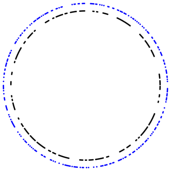
Figure 1: (Color online) Disposition of the $\sigma_{i}=1$ variables in a ring with $L=500$ sites. The inner circle (black) is an absorbing configuration of the extended majority-vote model with $\rho=0.49$. There are 92 clusters and the largest cluster comprises 19 sites. The outer circle (blue) shows a random configuration with the same density of 1’s. The total number of clusters is 255 and the largest one comprises 9 sites.

Although the majority-vote rule or, more generally, the frequency bias mechanism for cultural change [19] is a homogenizing assumption by which the agents become more similar to each other, the two-dimensional version of the above-described model does exhibit global polarization, i.e., a non-trivial stable multicultural regime in the thermodynamic limit [13, 17, 14]. This regime should exist in the one-dimensional version as well, since any sequence of two or more contiguous 1’s (or 0’s) is stable under the update rule. It should be noted that for the more popular variant of the majority-vote model, in which the state of the target site is not included in the majority reckoning, and ties are decided by choosing the opinion of the target agent at random with probability $1/2$, the only absorbing states in the thermodynamic limit are the two homogeneous configurations [20, 21]. As mentioned before, the inclusion of the target site in the calculation of the majority is actually the original definition of the majority-vote model as introduced in Refs. [11, 12]. Figure 1 illustrates an absorbing configuration of the extended majority-vote model together with a random configuration with the same density of 1’s. The larger number of clusters (domains) observed in the random configuration is due to the possibility of isolated sites, which are unstable under the majority-vote rule.

As usual, we represent the state of the agent at site $i$ of the ring by the binary variable $\sigma_{i}=0,1$ and so the configuration of the entire ring is denoted by $\sigma\equiv\left(\sigma_{1},\sigma_{2},\ldots,\sigma_{L}\right)$. The master equation that governs the time evolution of the probability distribution $P\left(\sigma,t\right)$ is given by

$$\frac{d}{dt}P\left(\sigma,t\right)=\sum_{i}\left[W_{i}\left(\tilde{\sigma}^{i}\right)P\left(\tilde{\sigma}^{i},t\right)-W_{i}\left(\sigma\right)P\left(\sigma,t\right)\right]$$ (1)

where $\tilde{\sigma}^{i}=\left(\sigma_{1},\ldots,1-\sigma_{i},\ldots,\sigma_{L}\right)$ and $W_{i}\left(\sigma\right)$ is the transition rate between configurations $\sigma$ and $\tilde{\sigma}^{i}$ [20, 21]. For the one-dimensional extended majority-vote model we have

$$W_{i}\left(\sigma\right)=\sigma_{i}\left(1-\sigma_{i-1}-\sigma_{i+1}\right)+\sigma_{i-1}\sigma_{i+1}$$ (2)

for $i=1,\ldots,L$. The boundary conditions are such that $\sigma_{0}=\sigma_{L}$ and $\sigma_{L+1}=\sigma_{1}$. To implement the $n$-site approximation up to $n=4$ we need to evaluate the following expectations

$$\frac{d}{dt}\left\langle\sigma_{i}\right\rangle=\left\langle\left(1-2\sigma_{i}\right)W_{i}\left(\sigma\right)\right\rangle,$$ (3)

$$\frac{d}{dt}\left\langle\sigma_{i}\sigma_{j}\right\rangle=2\left\langle\sigma_{j}\left(1-2\sigma_{i}\right)W_{i}\left(\sigma\right)\right\rangle,$$ (4)

$$\frac{d}{dt}\left\langle\sigma_{i}\sigma_{j}\sigma_{k}\right\rangle=3\left\langle\sigma_{j}\sigma_{k}\left(1-2\sigma_{i}\right)W_{i}\left(\sigma\right)\right\rangle,$$ (5)

$$\frac{d}{dt}\left\langle\sigma_{i}\sigma_{j}\sigma_{k}\sigma_{l}\right\rangle=4\left\langle\sigma_{j}\sigma_{k}\sigma_{l}\left(1-2\sigma_{i}\right)W_{i}\left(\sigma\right)\right\rangle$$ (6)

where all indexes are assumed distinct and we have introduced the notation $\left\langle\left(\ldots\right)\right\rangle\equiv\sum_{\sigma}\left(\ldots\right)P\left(\sigma,t\right)$. The $n$-site approximation is based on the calculation of this average by replacing the full joint distribution probability $P\left(\sigma,t\right)$ by a decomposed form that depends on the order $n$ of the approximation [see Eqs. (8), (11), (18) and (42)]. Of course, in the derivation of Eqs. (3)-(6), which generalize trivially to an arbitrary number of sites, we have assumed translational invariance, i.e., all sites are assumed equivalent.

3 Mean-field Analysis

In this section we study the one-dimensional extended majority-vote model using the well-known mean-field $n$-site approximation (see [22, 23, 24, 25]). The basic idea behind the $n$-site approximation is to rewrite the distribution $P\left(\sigma,t\right)$ in terms of elementary joint probabilities of $n$ contiguous sites only and then deriving a system of self-consistent equations for these probabilities. This key idea is expressed mathematically using the following equation which summarizes the approximation scheme,

$$P_{1\mid L-1}\left(\sigma_{i}\mid\sigma_{1},\ldots,\sigma_{L}\right)=P_{1\mid 2n-2}\left(\sigma_{i}\mid\sigma_{i-n+1},\ldots,\sigma_{i+n-1}\right)$$ (7)

where, of course, $\sigma_{i}$ does not appear in the arguments at the right of the $\mid$ delimiter in these conditionals. This procedure will be illustrated in the next subsections for $n=1$ to $n=4$. It is interesting to note that, except for the single-site approximation $n=1$, the states of any two sites are statistically dependent variables regardless of their positions in the ring.

3.1 The single-site approximation

This is the simplest mean-field scheme which assumes that the state of the agents at different sites are independent random variables so that

$$P\left(\sigma,t\right)=p_{1}\left(\sigma_{1},t\right)p_{1}\left(\sigma_{2},t\right)\ldots p_{1}\left(\sigma_{L},t\right)$$ (8)

and so it is only necessary to calculate the one-site distribution $p_{1}\left(\sigma_{i},t\right)$ to describe the dynamics completely. This can be done by noting that $\rho\equiv\langle\sigma_{i}\rangle_{t}=p_{1}\left(1,t\right)$ and using Eq. (3) to derive a self-consistent equation for $\rho$. The final result is simply

$$\dot{\rho}=\rho\left(-2\rho^{2}+3\rho-1\right)$$ (9)

with the notation $\dot{x}=dx/dt$. We note that $\rho$ contains the same information as the single-site probability distribution $p_{1}\left(\sigma_{i}\right)$ since $p_{1}\left(\sigma_{i}=1\right)=\rho$ and $p_{1}\left(\sigma_{i}=0\right)=1-\rho$. A straightforward stability analysis shows that there are three fixed points,

$$\rho_{1}=0,\quad\rho_{2}=1/2,\quad\rho_{3}=1,$$ (10)

with only $\rho_{1}$ and $\rho_{3}$ being stable. This means that only the homogeneous configurations are stable and so the single-site approximation completely fails to describe the steady state of the extended majority-vote model.

3.2 The pair approximation

Using Eq. (7) to write the full probability distribution in terms of the joint probability of two sites and omitting the time dependence we find

$$P\left(\sigma\right)=\frac{p_{2}\left(\sigma_{1},\sigma_{2}\right)p_{2}\left(\sigma_{2},\sigma_{3}\right)\ldots p_{2}\left(\sigma_{L-1},\sigma_{L}\right)p_{2}\left(\sigma_{L},\sigma_{1}\right)}{p_{1}\left(\sigma_{1}\right)p_{1}\left(\sigma_{2}\right)\ldots p_{1}\left(\sigma_{L-1}\right)p_{1}\left(\sigma_{L}\right)}$$ (11)

where $p_{1}\left(\sigma_{i}\right)=\sum_{\sigma_{j}}p_{2}\left(\sigma_{i},\sigma_{j}\right)$. To avoid overburden the notation we use the same notation for $p_{1}$ as done in the single-site approximation but the $p_{1}$ which appears in Eq. (11) is numerically distinct from that calculated in the previous section. This simplifying convention for the notation of probabilities will be used in the next sections as well.

Within this framework, it is only necessary to calculate $p_{2}\left(\sigma_{i},\sigma_{i+1}\right)$ to describe the dynamics of the model completely. This amounts to 4 variables, namely, $p_{2}\left(1,1\right),p_{2}\left(1,0\right),p_{2}\left(0,1\right)$ and $p_{2}\left(0,0\right)$, but use of the normalization condition and of the parity symmetry [$p_{2}\left(1,0\right)=p_{2}\left(0,1\right)$] allows us to reduce the number of independent variables to only 2. The first variable we pick is $\phi\equiv\left\langle\sigma_{i}\sigma_{i+1}\right\rangle=p_{2}\left(1,1\right)$ which is given by Eq. (4) with $j=i+1$. Next, noting that $p_{2}\left(1,0\right)=p_{1}\left(1\right)-p_{2}\left(1,1\right)=\rho-\phi$ we pick $\rho$, given by Eq. (3), as the second independent variable. Carrying out the averages in the right-hand sides of Eqs. (3) and (4) using the decomposition (11) yields

$$\dot{\rho}=\frac{\left(\rho-\phi\right)^{2}\left(2\rho-1\right)}{2\rho\left(1-\rho\right)}$$ (12)

and

$$\dot{\phi}=\frac{\left(\rho-\phi\right)^{2}}{1-\rho}.$$ (13)

The steady-state condition $\dot{\phi}=\dot{\rho}=0$ as well as the numerical integration of these equations yields $\rho=\phi$ for $t\to\infty$, with $\rho$ determined by the value of the initial condition $\rho\left(t=0\right)=\rho_{0}$ and $\phi\left(t=0\right)=\rho_{0}^{2}$. We note that this result implies that $p_{2}\left(1,0\right)=p_{2}\left(0,1\right)=0$, meaning that the number of interfaces between clusters, i.e., of contiguous sites in different states at the steady state, is not extensive. This prediction is not correct as indicated by the higher-order approximations and by the simulation data. Despite this incorrect prediction, the pair approximation explains the most remarkable aspect of the extended majority-vote model, namely, the ergodicity breaking reflected by the infinity of distinct absorbing configurations.

The imposition of the steady-state condition is not sufficient to determine the equilibrium solution $\bar{\rho}=\bar{\phi}$ because there is a continuum of fixed points characterized by the function $\bar{\rho}\left(\rho_{0}\right)$. In order to obtain this function or map, we revert to the original variable $x\equiv p_{2}\left(1,0\right)=\rho-\phi$, and rewrite Eqs. (12) and (13) as

$$\dot{\rho}=\frac{x^{2}\left(2\rho-1\right)}{2\rho\left(1-\rho\right)},$$ (14)

$$\dot{x}=-\frac{x^{2}}{2\rho\left(1-\rho\right)}.$$ (15)

from which we can immediately obtain the integral equation

$$\int_{x_{0}}^{x\left(t\right)}dx^{\prime}=-\int_{\rho_{0}}^{\rho\left(t\right)}\frac{d\rho^{\prime}}{2\rho^{\prime}-1}.$$ (16)

As the stationary regime is obtained in the limit $t\rightarrow\infty$, we define $\bar{\rho}\left(\rho_{0}\right)\equiv\rho\left(t\rightarrow\infty\right)$. In addition, using $x_{0}=\rho_{0}\left(1-\rho_{0}\right)$ and $x\left(t\rightarrow\infty\right)=0$ (steady-state condition) we find

$$\bar{\rho}\left(\rho_{0}\right)=\frac{1}{2}\left[1+\left(2\rho_{0}-1\right)e^{2\rho_{0}\left(1-\rho_{0}\right)}\right].$$ (17)

This equation is identical to that derived for the non-conservative voter model in the case the voter changes opinion only when confronted by a unanimity of opposite-opinion neighbors[18]. Figure 2 shows this steady-state solution together with the results of the simulations for a ring with $L=10^{4}$ sites. Despite the incorrect prediction ($\bar{\phi}=\bar{\rho}$), Eq. (17) yields a remarkably good quantitative agreement with the density $\rho$ obtained from the simulations. However, as we will show next the (supposedly) exact expression for $\bar{\rho}$ is much simpler than Eq. (17).

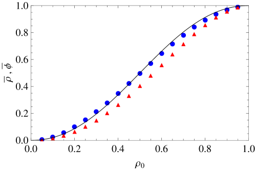
Figure 2: (Color online) The fraction of sites in state $1$ at equilibrium, $\bar{\rho}$ (filled circles), and the probability that two neighbors are in state $1$ at equilibrium, $\bar{\phi}$ (filled triangles) as functions of the initial fraction of sites in state $1$, $\rho_{0}$. The solid line is the result of the pair approximation for which $\bar{\rho}=\bar{\phi}$ given by Eq. (17). The initial condition is $\rho=\rho_{0}$ and $\phi=\rho_{0}^{2}$. The symbols show the results of the simulations for a ring of size $L=10^{4}$ and $10^{6}$ independent samples.

3.3 The $3$-site approximation

In this scheme the decomposition of $P\left(\sigma\right)$ is

$$P\left(\sigma\right)=\frac{p_{3}\left(\sigma_{1},\sigma_{2},\sigma_{3}\right)p_{3}\left(\sigma_{2},\sigma_{3},\sigma_{4}\right)\ldots p_{3}\left(\sigma_{L},\sigma_{1},\sigma_{2}\right)}{p_{2}\left(\sigma_{1},\sigma_{2}\right)p_{2}\left(\sigma_{2},\sigma_{3}\right)\ldots p_{2}\left(\sigma_{L},\sigma_{1}\right)}$$ (18)

where $p_{2}\left(\sigma_{i},\sigma_{i+1}\right)=\sum_{\sigma_{i+2}}p_{3}\left(\sigma_{i},\sigma_{i+1},\sigma_{i+2}\right)$. The goal here is to calculate the 9 probability values $p_{3}\left(\sigma_{i},\sigma_{i+1},\sigma_{i+2}\right)$ with $\sigma_{k}=0,1$. As before, use of the normalization condition and of the parity symmetry give us 6 variables to be determined using appropriate linear combinations of Eqs. (3)-(6). We choose the following variables

$$\eqalign{x_{0}=p_{3}\left(0,0,0\right),\qquad~{}~{}x_{1}=p_{3}\left(1,0,0\right),\qquad~{}x_{2}=p_{3}\left(1,1,0\right),\cr x_{1C}=p_{3}\left(0,1,0\right),\qquad x_{2C}=p_{3}\left(1,0,1\right),\qquad x_{3}=p_{3}\left(1,1,1\right).}$$ (19)

which are given by the expectations $x_{1}=\left\langle\sigma_{i}\right\rangle-\left\langle\sigma_{i}\sigma_{i+1}\right\rangle-\left\langle\sigma_{i}\sigma_{i+2}\right\rangle+\left\langle\sigma_{i}\sigma_{i+1}\sigma_{i+2}\right\rangle$, $x_{2}=\left\langle\sigma_{i}\sigma_{i+1}\right\rangle-\left\langle\sigma_{i}\sigma_{i+1}\sigma_{i+2}\right\rangle$, $x_{3}=\left\langle\sigma_{i}\sigma_{i+1}\sigma_{i+2}\right\rangle$, and so on.

3.3.1 Mean-field equations.

Evaluating the averages in Eqs. (3)-(6) using the decomposition (18) yields

$$\eqalign{\dot{x}_{1}=\frac{1}{3}\frac{x_{1C}}{x_{1C}+x_{2}}\left(x_{2C}-x_{1}\right),\qquad~{}~{}~{}~{}~{}~{}~{}~{}~{}\dot{x}_{2}=\frac{1}{3}\frac{x_{2C}}{x_{2C}+x_{1}}\left(x_{1C}-x_{2}\right),\cr\dot{x}_{1C}=-\frac{1}{3}\frac{x_{1C}}{x_{2C}+x_{1}}\left(3x_{2C}+x_{1}\right),\qquad~{}~{}~{}\dot{x}_{2C}=-\frac{1}{3}\frac{x_{2C}}{x_{1C}+x_{2}}\left(3x_{1C}+x_{2}\right),\cr\dot{x}_{0}=\frac{1}{3}\frac{x_{1C}}{x_{1C}+x_{2}}\left(x_{1C}+2x_{1}+x_{2}\right),\qquad\dot{x}_{3}=\frac{1}{3}\frac{x_{2C}}{x_{2C}+x_{1}}\left(x_{2C}+x_{1}+2x_{2}\right).}$$ (20)

The steady state is given by $x_{1C}=x_{2C}=0$, i.e., $p_{3}\left(0,1,0\right)=p_{3}\left(1,0,1\right)=0$ which, in contrast to the situation we found in the analysis of the pair approximation, reflects the physical requirement that absorbing configurations cannot exhibit isolated sites. As we are still left with $4$ undetermined variables after applying the steady-state condition, we need an alternative method to characterize the steady state. Somewhat surprisingly, in this case we will be able to solve the dynamics analytically, a feat that seems unfeasible in the case of the pair approximation.

In fact, what makes the system of nonlinear coupled equations (20) solvable is the observation that $y\equiv x_{1C}+x_{2}=x_{2C}+x_{1}=p_{2}\left(1,0\right)$, so the denominators in the r.h.s. of all those equations are identical. In addition, we note that $x_{0}$ does not affect the other 5 variables so we can first solve for them and then return to the equation for $x_{0}$ to complete the solution of the system (20).

Introducing the auxiliary variables $z_{1}=x_{1C}+x_{2C}$, $z_{2}=x_{1C}-x_{2C}$, and recalling that $\rho=x_{1}+x_{2}+x_{2C}+x_{3}$ we reduce Eqs. (20) to

$$\dot{y}=-\frac{z_{1}}{3},\qquad\dot{z}_{1}=-\frac{z_{1}}{3}-\frac{z_{1}^{2}-z_{2}^{2}}{3y},\qquad\dot{z}_{2}=-\frac{z_{2}}{3},\qquad\dot{\rho}=-\frac{z_{2}}{3},$$ (21)

where we have omitted the equation for $x_{0}$. The last two equations can be immediately solved and yield

$$z_{2}\left(t\right)=\rho_{0}\left(1-\rho_{0}\right)\left(1-2\rho_{0}\right)e^{-\frac{1}{3}t},$$ (22)

$$\rho\left(t\right)=\rho_{0}^{2}\left(3-2\rho_{0}\right)+\rho_{0}\left(1-\rho_{0}\right)\left(1-2\rho_{0}\right)e^{-\frac{1}{3}t},$$ (23)

Hence in the asymptotic limit $t\rightarrow\infty$ we obtain

$$\bar{\rho}\left(\rho_{0}\right)=\rho_{0}^{2}\left(3-2\rho_{0}\right)$$ (24)

and $\bar{z}_{2}=0$, as expected, since both $x_{1C}$ and $x_{2C}$ vanish at the steady state. For $\rho_{0}\to 0$ or $\rho_{0}\to 1$ the pair approximation estimate of $\bar{\rho}$ given by Eq. (17) reduces to Eq.  (24) in a first order approximation in $\rho_{0}$ or $1-\rho_{0}$. Equation (24) describes the simulation data perfectly as illustrated in Fig. 3 and, as already mentioned, we believe it gives the exact value for the steady-state density of 1s of the one-dimensional majority-vote model.

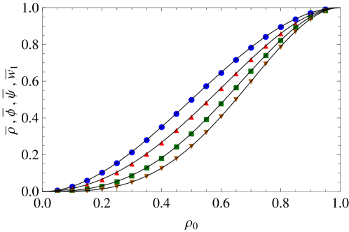
Figure 3: (Color online) The solid lines are the analytical results for the steady-state measures obtained with the $4$-site approximation while the symbols represent the results of the simulations for a ring of size $L=10^{4}$ and $10^{6}$ independent samples. The convention is (from top to bottom) $\bar{\rho}\left(\rho_{0}\right)$ (circles), $\bar{\phi}\left(\rho_{0}\right)$ (triangles), $\bar{\psi}\left(\rho_{0}\right)$ (squares) and $\bar{w}_{1}\left(\rho_{0}\right)$ (upside down triangles). The upper three curves are identical for the $3$-site approximation.

The explicit calculation of the remaining two unknowns $y$ and $z_{1}$ using Eqs.  (21) is not too involved and their knowledge will allow us to evaluate other quantities of interest, such as $\phi$ and other high-order correlations. We begin by introducing the auxiliary variables $\omega_{1}=z_{1}/y$ and $\omega_{2}=z_{2}/y$ which satisfy the equations

$$\dot{\omega}_{1}=-\frac{1}{3}\omega_{1}+\frac{1}{3}\omega_{2}^{2},\qquad\dot{\omega}_{2}=-\frac{1}{3}\omega_{2}+\frac{1}{3}\omega_{1}\omega_{2}.$$ (25)

Next, we define $\alpha=\omega_{1}^{2}-\omega_{2}^{2}$ which is given by $\dot{\alpha}=-2\alpha/3$ and so

$$\alpha\left(t\right)=\alpha_{0}e^{-\frac{2t}{3}},$$ (26)

with $\alpha_{0}=4\rho_{0}\left(1-\rho_{0}\right)$. At this point we can readily write an explicit equation for $z_{1}$ in terms of $y$,

$$z_{1}\left(t\right)=e^{-\frac{t}{3}}\sqrt{z_{0}^{2}+\alpha_{0}y^{2}\left(t\right)},$$ (27)

where we used the fact that $z_{1}\geq 0$ and that $z_{2}$ is given by Eq. (22). Now, inserting this expression in the equation for $y$ [see Eq.  (21)] results in an easily solvable integral,

$$\int_{y_{0}}^{y}\frac{dy^{\prime}}{\sqrt{m_{0}^{2}+y^{\prime 2}}}=\log{\left(\frac{y+\sqrt{m_{0}^{2}+y^{2}}}{y_{0}+\sqrt{m_{0}^{2}+y_{0}^{2}}}\right)},$$ (28)

with $m_{0}^{2}=z_{0}^{2}/\alpha_{0}$ and $y_{0}=\rho_{0}\left(1-\rho_{0}\right)$. Finally, carrying out the integration yields

$$y\left(t\right)= \frac{1}{2}\left(y_{0}+\sqrt{m_{0}^{2}+y_{0}^{2}}\right)\exp{\left[-\sqrt{\alpha_{0}}\left(1-e^{-\frac{t}{3}}\right)\right]}$$ (29)

$$-\frac{1}{2}\frac{m_{0}^{2}}{y_{0}+\sqrt{m_{0}^{2}+y_{0}^{2}}}\exp{\left[\sqrt{\alpha_{0}}\left(1-e^{-\frac{t}{3}}\right)\right]}.$$

In the limit $t\to\infty$ this equation reduces to

$$\bar{y}\left(\rho_{0}\right) = \rho_{0}\left(1-\rho_{0}\right)\cosh{\left[2\sqrt{\rho_{0}\left(1-\rho_{0}\right)}\right]}$$ (30)

$$-\frac{1}{2}\sqrt{\rho_{0}\left(1-\rho_{0}\right)}\sinh{\left[2\sqrt{\rho_{0}\left(1-\rho_{0}\right)}\right]}$$

which exhibits the symmetry $\bar{y}\left(\rho_{0}\right)=\bar{y}\left(1-\rho_{0}\right)$.

To conclude the solution of the system of equations (20) we need now to determine $x_{0}$. The easiest way to do that is to rewrite the equation for $x_{0}$ in (20) as

$$\dot{x}_{0}=-2\dot{y}+\frac{1}{2}\left(\dot{z}_{1}-3\dot{z}_{2}\right)$$ (31)

which can be immediately integrated to yield

$$x_{0}\left(t\right)=x_{0}\left(0\right)-2\left[y\left(t\right)-y_{0}\right]+\frac{1}{2}\left[z_{1}\left(t\right)-z_{1}\left(0\right)\right]-\frac{3}{2}\left[z_{2}\left(t\right)-z_{2}\left(0\right)\right].$$ (32)

In the asymptotic limit $x_{0}\left(t\to\infty\right)\equiv\bar{\psi}_{-1}$ we find

$$\bar{\psi}_{-1}\left(\rho_{0}\right)=\left(1+2\rho_{0}\right)\left(1-\rho_{0}\right)^{2}-2\bar{y}\left(\rho_{0}\right).$$ (33)

3.3.2 Simple steady-sate expectations.

At this stage we should be able to express any quantity characterizing the ring configuration at time $t$ in terms of the time-dependent variables $\rho$, $z_{2}$, $y$ and $z_{1}$. However, we will focus here only in the steady-state regime ($t\to\infty$) for which only $\rho$ and $y$ contribute since $\bar{z}_{1}=\bar{z}_{2}=0$.

The most interesting expectations are those whose time evolution are defined by Eqs.  (3)-(6) in the case the indexes are associated to contiguous sites. We begin with $\phi=\left\langle\sigma_{i}\sigma_{i+1}\right\rangle=x_{2}+x_{3}$, and recall that $\rho=\left\langle\sigma_{i}\right\rangle=x_{1}+x_{2}+x_{2C}+x_{3}$ and $y=x_{1}+x_{2C}$ so that $\phi=\rho-y$. Then at the steady state we find

$$\bar{\phi}\left(\rho_{0}\right)=\rho_{0}^{2}\left(3-2\rho_{0}\right)-\bar{y}\left(\rho_{0}\right).$$ (34)

Next we note that $\psi\equiv\left\langle\sigma_{i}\sigma_{i+1}\sigma_{i+2}\right\rangle=x_{3}=\rho-2y+\left(z_{1}+z_{2}\right)/2$ and so

$$\bar{\psi}\left(\rho_{0}\right)=\rho_{0}^{2}\left(3-2\rho_{0}\right)-2\bar{y}\left(\rho_{0}\right).$$ (35)

These two steady-state expectations, which are shown in Fig. 3, describe the simulation data perfectly. Expectations involving more than three contiguous sites must be decomposed so as to be described by the $3$-site approximation. Of particular interest is the 4-site expectation $w_{1}\equiv\left\langle\sigma_{i}\sigma_{i+1}\sigma_{i+2}\sigma_{i+3}\right\rangle=p_{4}\left(1,1,1,1\right)$, which in the 3-site approximation scheme becomes $w_{1}=p_{3}^{2}\left(1,1,1\right)/p_{2}\left(1,1\right)$ so that $\bar{w}_{1}\left(\rho_{0}\right)=\bar{\psi}^{2}/\bar{\phi}$ at the steady state. In the scale of fig. 3 this result is indistinguishable from the simulation data or from their counterpart calculated with the $4$-site approximation (see fig. 4).

For completeness, let us calculate $\phi_{-1}\equiv p_{2}\left(0,0\right)=x_{1}+x_{0}$ at the steady state. Since $x_{0}$ is given by Eq. (33) and $x_{1}=y-\left(z_{1}-z_{2}\right)/2$ we find

$$\bar{\phi}_{-1}\left(\rho_{0}\right)=\left(1+2\rho_{0}\right)\left(1-\rho_{0}\right)^{2}-\bar{y}\left(\rho_{0}\right).$$ (36)

The fact that the dynamics is invariant to the interchange of 1s and 0s provided that we change $\rho_{0}$ to $1-\rho_{0}$ is expressed by the easily verifiable identities $\bar{\rho}\left(1-\rho_{0}\right)=1-\bar{\rho}\left(\rho_{0}\right)$, $\bar{\phi}\left(\rho_{0}\right)=\bar{\phi}_{-1}\left(1-\rho_{0}\right)$, and $\bar{\psi}\left(\rho_{0}\right)=\bar{\psi}_{-1}\left(1-\rho_{0}\right)$. Of course, this symmetry holds for all orders $n$ of the $n$-site approximation scheme and we will resort to it to abbreviate the calculations of the $4$-site approximation in Sect. 3.4.

3.3.3 Probability of clusters of length $m$.

A more informative quantity is the probability of finding a cluster of $m>1$ sites in an absorbing configuration. There are only two possibilities for such a cluster: (a) a site in state $\sigma_{i}=0$ followed by $m$ sites in states $\sigma_{i+1}=\sigma_{i+2}\ldots\sigma_{i+m}=1$ which are then followed by another site in state $\sigma_{i+m+1}=0$ and (b) a site in state $\sigma_{i}=1$ followed by $m$ sites in states $\sigma_{i+1}=\sigma_{i+2}\ldots\sigma_{i+m}=0$ which are then followed by another site in state $\sigma_{i+m+1}=1$. The probability of these configurations happening in an absorbing configuration can be easily derived using the decomposition (18) and yields

$$P^{(3)}_{cl}\left(m\right)=\frac{p_{3}^{2}\left(0,1,1\right)}{p_{2}\left(1,1\right)}\left[\frac{p_{3}\left(1,1,1\right)}{p_{2}\left(1,1\right)}\right]^{m-2}+\frac{p_{3}^{2}\left(1,0,0\right)}{p_{2}\left(0,0\right)}\left[\frac{p_{3}\left(0,0,0\right)}{p_{2}\left(0,0\right)}\right]^{m-2}.$$ (37)

To rewrite this expression in terms of more elementary steady-state quantities we recall that $p_{3}\left(1,0,0\right)=p_{2}\left(0,0\right)-p_{3}\left(0,0,0\right)$ and $p_{3}\left(0,1,1\right)=p_{2}\left(1,1\right)-p_{3}\left(1,1,1\right)$ so that

$$P^{(3)}_{cl}\left(\rho_{0},m\right)=\frac{\left(\bar{\phi}-\bar{\psi}\right)^{2}}{\bar{\phi}}\left(\frac{\bar{\psi}}{\bar{\phi}}\right)^{m-2}+\frac{\left(\bar{\phi}_{-1}-\bar{\psi}_{-1}\right)^{2}}{\bar{\phi}_{-1}}\left(\frac{\bar{\psi}_{-1}}{\bar{\phi}_{-1}}\right)^{m-2}.$$ (38)

The 3-site approximation estimate for the probability of finding clusters of length $m$ given by this equation is presented in Figs. 5 and 6 together with the results of the simulations and the estimate of the 4-site approximation. We will postpone the discussion of the physical implications of the results presented in these figures to Sect.  4.

3.3.4 Two-site correlations.

Knowledge of the two-site correlations defined by

$$\textrm{corr}\left(\sigma_{i},\sigma_{i+j}\right)=\langle\sigma_{i}\sigma_{i+j}\rangle-\langle\sigma_{i}\rangle\langle\sigma_{i+j}\rangle$$ (39)

is very useful to determine the validity of the approximations. Since all sites are equivalent we have $\langle\sigma_{i}\rangle=\langle\sigma_{i+j}\rangle=\bar{\rho}\left(\rho_{0}\right)$ regardless of the order $n$ of the approximation. Some two-site expectations follow straightforwardly from the previous results, namely, $\langle\sigma_{i}\sigma_{i}\rangle_{\left(3\right)}=\bar{\rho}$, $\langle\sigma_{i}\sigma_{i+1}\rangle_{\left(3\right)}=\bar{\phi}$ and $\langle\sigma_{i}\sigma_{i+2}\rangle_{\left(3\right)}=\bar{\psi}$. The first nontrivial two-site expectation is

$$\left\langle\sigma_{i}\sigma_{i+3}\right\rangle_{\left(3\right)} = \sum_{\sigma_{i+1},\sigma_{i+2}}P\left(\sigma_{i}=1,\sigma_{i+1},\sigma_{i+2},\sigma_{i+3}=1\right)$$ (40)

$$= \frac{\bar{\psi}^{2}}{\bar{\phi}}+\frac{\left(\bar{\phi}_{-1}-\bar{\psi}_{-1}\right)^{2}}{\bar{\phi}_{-1}}$$

where we have decomposed the 4-site probability in terms of the elementary 3-site probabilities. Note that the sum has two non-vanishing terms only, since $P\left(1,0,1,1\right)=P\left(1,1,0,1\right)=0$. Applying the very same procedure to calculate $\left\langle\sigma_{i}\sigma_{i+4}\right\rangle$ yields

$$\left\langle\sigma_{i}\sigma_{i+4}\right\rangle_{\left(3\right)}=\left(\frac{\bar{\psi}}{\bar{\phi}}\right)^{2}\bar{\psi}+2\frac{\left(\bar{\phi}_{-1}-\bar{\psi}_{-1}\right)^{2}}{\bar{\phi}_{-1}}+\left(\frac{\bar{\phi}_{-1}-\bar{\psi}_{-1}}{\bar{\phi}_{-1}}\right)^{2}\bar{\psi}_{-1}.$$ (41)

In this case only 4 terms give nonzero contributions to the sum over the middle sites. Equations (40) and (41) clarify a fact that is often unappreciated, namely, regardless of their position in the ring, the sites are always treated as statistically dependent variables within the $n$-site approximation scheme for $n>1$.

3.4 The $4$-site approximation

In the $4$-site approximation framework the decomposition of $P\left(\sigma\right)$ is given by the prescription

$$P\left(\sigma\right)=\frac{p_{4}\left(\sigma_{1},\sigma_{2},\sigma_{3},\sigma_{4}\right)p_{4}\left(\sigma_{2},\sigma_{3},\sigma_{4},\sigma_{5}\right)\ldots p_{4}\left(\sigma_{L},\sigma_{1},\sigma_{2},\sigma_{3}\right)}{p_{3}\left(\sigma_{1},\sigma_{2},\sigma_{3}\right)p_{3}\left(\sigma_{2},\sigma_{3},\sigma_{4}\right)\ldots p_{3}\left(\sigma_{L},\sigma_{1},\sigma_{2}\right)}$$ (42)

where $p_{3}\left(\sigma_{i},\sigma_{i+1},\sigma_{i+2}\right)=\sum_{\sigma_{i+3}}p_{4}\left(\sigma_{i},\sigma_{i+1},\sigma_{i+2},\sigma_{i+3}\right)$. Full determination of the joint probability $p_{4}\left(\sigma_{i},\sigma_{i+1},\sigma_{i+2},\sigma_{i+3}\right)$ requires the calculation of 16 unknowns, but the normalization condition and the parity symmetry allows us to reduce this number to the following 10 unknowns

$$\eqalign{w_{-1}=p_{4}\left(0,0,0,0\right),\\ x_{1}=p_{4}\left(1,0,0,0\right),\quad x_{2}=p_{4}\left(0,1,0,0\right),\\ y_{1}=p_{4}\left(1,1,0,0\right),\quad y_{2}=p_{4}\left(1,0,1,0\right),\quad y_{3}=p_{4}\left(1,0,0,1\right),\quad y_{4}=p_{4}\left(0,1,1,0\right),\\ z_{1}=p_{4}\left(1,1,1,0\right),\quad z_{2}=p_{4}\left(1,1,0,1\right),\\ w_{1}=p_{4}\left(1,1,1,1\right).}$$ (48)

As usual, Eqs. (3)-(6) allow us to derive the equations for all these unknowns. For example, $z_{1}=\langle\sigma_{i}\sigma_{i+1}\sigma_{i+2}\rangle-\langle\sigma_{i}\sigma_{i+1}\sigma_{i+2}\sigma_{i+3}\rangle$, $w_{1}=\langle\sigma_{i}\sigma_{i+1}\sigma_{i+2}\sigma_{i+3}\rangle$ and so on.

3.4.1 Mean-field equation

Evaluation of the averages in Eqs. (3)-(6) using the decomposition (42) results in the following set of equations

$$\eqalign{\dot{w}_{-1}=\frac{x_{2}}{2}\left(1+\frac{x_{1}}{x_{2}+y_{1}}\right),\\ \dot{x}_{1}=\frac{1}{4}\left[\frac{x_{2}}{x_{2}+y_{1}}\left(y_{3}-x_{1}\right)+y_{2}\right],\qquad\dot{x}_{2}=\frac{1}{4}\left(\frac{y_{2}^{2}}{y_{2}+z_{2}}-\frac{x_{2}y_{2}}{x_{2}+y_{2}}-x_{2}\right),\\ \dot{y}_{1}=\frac{y_{2}}{4}\left(\frac{x_{2}}{x_{2}+y_{2}}+\frac{z_{2}}{y_{2}+z_{2}}\right),\qquad~{}~{}~{}\dot{y}_{2}=-\frac{y_{2}}{4}\left(\frac{y_{2}}{x_{2}+y_{2}}+\frac{y_{2}}{y_{2}+z_{2}}+2\right),\\ \dot{y}_{3}=-\frac{1}{2}\frac{x_{2}y_{3}}{x_{2}+y_{1}},\qquad~{}~{}~{}~{}~{}~{}~{}~{}~{}~{}~{}~{}~{}~{}~{}~{}~{}~{}~{}~{}~{}\dot{y}_{4}=-\frac{1}{2}\frac{y_{4}z_{2}}{y_{1}+z_{2}},\\ \dot{z}_{1}=\frac{1}{4}\left[\frac{z_{2}}{y_{1}+z_{2}}\left(y_{4}-z_{1}\right)+y_{2}\right],\qquad~{}\dot{z}_{2}=\frac{1}{4}\left(\frac{y_{2}^{2}}{x_{2}+y_{2}}-\frac{y_{2}z_{2}}{y_{2}+z_{2}}-z_{2}\right),\\ \dot{w}_{1}=\frac{z_{2}}{2}\left(1+\frac{z_{1}}{y_{1}+z_{2}}\right).}$$ (55)

As the variables $w_{-1}$ and $w_{1}$ do not affect the other variables and the consistency conditions

$$\sum_{\sigma_{x_{1}},\sigma_{x_{2}}}p_{4}\left(1,1,\sigma_{x_{1}},\sigma_{x_{2}}\right) = \sum_{\sigma_{x_{1}},\sigma_{x_{2}}}p_{4}\left(\sigma_{x_{1}},1,1,\sigma_{x_{2}}\right),$$ (56a)

$$\sum_{\sigma_{x_{1}},\sigma_{x_{2}}}p_{4}\left(1,0,\sigma_{x_{1}},\sigma_{x_{2}}\right) = \sum_{\sigma_{x_{1}},\sigma_{x_{2}}}p_{4}\left(\sigma_{x_{1}},1,0,\sigma_{x_{2}}\right),$$ (56b)

result in the simple relations,

$$y_{1}+z_{2}=y_{4}+z_{1},\qquad x_{1}+y_{3}=x_{2}+y_{1},$$ (56be)

from where we can eliminate $x_{2}$ and $y_{1}$, we are actually left with a system of 6 coupled equations for the variables $x_{1},y_{1},y_{3},y_{4},z_{1}$ and $z_{2}$. (We note that Eqs. (56a) and (56b) merely exhibit alternative ways of expressing $p_{2}\left(1,1\right)$ and $p_{2}\left(1,0\right)$, respectively.)

Introducing the linear transformation

$$\alpha_{\pm}=y_{4}\pm z_{1},\qquad\eta_{\pm}=y_{2}\pm z_{2},\qquad\delta_{\pm}=y_{3}\pm x_{1},$$ (56bf)

we obtain the closed set of equations

$$\eqalign{\dot{\alpha}_{+}=\frac{1}{4}\eta_{-},\qquad~{}~{}~{}~{}~{}~{}~{}~{}~{}~{}~{}~{}~{}~{}~{}~{}\dot{\alpha}_{-}=-\frac{1}{4}\left[\eta_{+}+\frac{\alpha_{-}}{\alpha_{+}}\left(\eta_{+}-\eta_{-}\right)\right],\\ \dot{\eta}_{+}=-\frac{1}{4}\left(2\eta_{+}+\eta_{-}\right),\qquad~{}~{}~{}\dot{\eta}_{-}=-\frac{1}{8}\left[\frac{\eta_{+}^{2}+4\eta_{+}\eta_{-}+\eta_{-}^{2}}{\eta_{+}}-\frac{\left(\eta_{+}+\eta_{-}\right)^{2}}{\alpha_{+}-\eta_{+}-\delta_{+}}\right],\\ \dot{\delta}_{+}=\frac{1}{4}\left(\alpha_{+}+\eta_{-}-\delta_{+}\right),\qquad\dot{\delta}_{-}=\frac{1}{4}\left[\alpha_{+}-\eta_{+}-\delta_{+}+\frac{\delta_{-}}{\delta_{+}}\left(2\alpha_{+}-2\delta_{+}-\eta_{+}+\eta_{-}\right)\right].}$$ (56bj)

Although this system might look formidable, its solution is not very involved. We begin by eliminating $\eta_{-}$ in the equations for $\alpha_{+}$ and $\delta_{+}$ in order to get

$$\dot{\delta}_{+}+\frac{1}{4}\delta_{+}=\dot{\alpha}_{+}+\frac{1}{4}\alpha_{+}.$$ (56bk)

The auxiliary variable $f=\alpha_{+}-\delta_{+}$ satisfies $\dot{f}=-\frac{1}{4}f$, whose solution is

$$f\left(t\right)=\left(\alpha_{+0}-\delta_{+0}\right)e^{-\frac{t}{4}}=\rho_{0}\left(1-\rho_{0}\right)\left(2\rho_{0}-1\right)e^{-\frac{t}{4}}.$$ (56bl)

This explicit solution for $f$ in terms of $\rho_{0}$ and $t$ allows us to consider the equations for $\eta_{\pm}$ as a closed subset of equations which can be solved as follows. The change of variables

$$\omega=\frac{\eta_{+}+\eta_{-}}{\eta_{+}},\qquad\gamma=\frac{\eta_{+}+\eta_{-}}{f-\eta_{+}},$$ (56bm)

leads to the much simpler equations

$$\dot{\omega}=-\frac{1}{4}\omega+\frac{1}{8}\omega^{2}+\frac{1}{8}\gamma\omega,\qquad\dot{\gamma}=-\frac{1}{4}\gamma-\frac{1}{8}\gamma^{2}-\frac{1}{8}\gamma\omega$$ (56bn)

which imply that $d\left(\gamma\omega\right)/dt=-\frac{1}{2}\gamma\omega$. Hence

$$\gamma\left(t\right)\omega\left(t\right)=-4\rho_{0}\left(1-\rho_{0}\right)e^{-\frac{t}{2}},$$ (56bo)

where we have used $\gamma\left(t=0\right)=-2\rho_{0}$ and $\omega\left(t=0\right)=2\left(1-\rho_{0}\right)$. Inserting this expression back into the equation for $\gamma$ we obtain a Ricatti equation, whose exact solution is [26]

$$\gamma\left(t\right)=-2\sqrt{\rho_{0}\left(1-\rho_{0}\right)}e^{-\frac{t}{4}}\tanh{\left[\Xi\left(\rho_{0},t\right)\right]}$$ (56bp)

with

$$\Xi\left(\rho_{0},t\right)=\tanh^{-1}{\left(\frac{\rho_{0}}{1-\rho_{0}}\right)^{1/2}}+\sqrt{\rho_{0}\left(1-\rho_{0}\right)}\left(e^{-\frac{t}{4}}-1\right).$$ (56bq)

Since we have found explicit solutions for $\gamma$ and $\omega$ we can easily revert to the original variables $\eta_{+}=f\gamma/\left(\gamma+\omega\right)$ and $\eta_{-}=f\gamma\left(\omega-1\right)/\left(\gamma+\omega\right)$ so as to write

$$\eta_{+}=-\rho_{0}\left(1-\rho_{0}\right)\left(2\rho_{0}-1\right)e^{-\frac{t}{4}}\sinh^{2}{\left[\Xi\left(\rho_{0},t\right)\right]}$$ (56br)

and

$$\eta_{-}=-\eta_{+}-\left[\rho_{0}\left(1-\rho_{0}\right)\right]^{3/2}\left(2\rho_{0}-1\right)e^{-\frac{t}{2}}\sinh{\left[2\Xi\left(\rho_{0},t\right)\right]}.$$ (56bs)

At this point we can immediately obtain $\alpha_{+}$, given in Eq. (56bj), through a brute-force integration

$$\alpha_{+}\left(t\right) = \frac{1}{2}\rho_{0}\left(1-\rho_{0}\right)\left(2\rho_{0}-1\right)e^{-\frac{t}{4}}$$ (56bt)

$$+\frac{1}{2}\rho_{0}\left(1-\rho_{0}\right)\left(2-e^{-\frac{t}{4}}\right)\cosh{\left[2\sqrt{\rho_{0}\left(1-\rho_{0}\right)}\left(1-e^{-\frac{t}{4}}\right)\right]}$$

$$-\frac{1}{2}\sqrt{\rho_{0}\left(1-\rho_{0}\right)}\left[1-2\rho_{0}\left(1-\rho_{0}\right)e^{-\frac{t}{4}}\right]\sinh{\left[2\sqrt{\rho_{0}\left(1-\rho_{0}\right)}\left(1-e^{-\frac{t}{4}}\right)\right]}.$$

Note that $\alpha_{+}\left(t\to\infty\right)=\bar{y}\left(\rho_{0}\right)$ calculated within the 3-site approximation [see Eq. (30)]. Together with the expression for $f$ given in Eq. (56bl), this result allows to obtain $\delta_{+}=\alpha_{+}-f$. Hence, to complete the solution of the system (56bj) we need now to determine $\alpha_{-}$ and $\delta_{-}$. This is achieved as follows.

The auxiliary variable $\chi=\frac{\alpha_{-}}{\alpha_{+}}$ satisfies

$$\dot{\chi}=-\frac{1}{4}\left(1+\chi\right)\frac{\eta_{+}}{\alpha_{+}},$$ (56bu)

whose solution is simply

$$\chi\left(t\right)=2\left(1-\rho_{0}\right)e^{-G\left(t\right)}-1$$ (56bv)

where we have used $\chi\left(t=0\right)=1-2\rho_{0}$ and

$$G\left(t\right)=\frac{1}{4}\int_{0}^{t}\frac{\eta_{+}\left(t^{\prime}\right)}{\alpha_{+}\left(t^{\prime}\right)}dt^{\prime}.$$ (56bw)

Hence $\alpha_{-}\left(t\right)=\alpha_{+}\left(t\right)\chi\left(t\right)$ where the factors in the product are given by Eqs. (56bt) and (56bv). To solve for the last unknown $\delta_{-}$ we resort to a shortcut. Considering the definitions of $\delta_{-}$ and $\alpha_{-}$ in terms of the elementary probabilities given in (48) we see that they are related by the transformation $1\leftrightarrow 0$ and so $\delta_{-}\left(t,\rho_{0}\right)=\alpha_{-}\left(t,1-\rho_{0}\right)$. This concludes the solution of the system (56bj), but we note that since we are not able to solve analytically the integral in Eq. (56bw) the situation here is not as satisfying as for the 3-site approximation. Most fortunately, that integral does not appear in the expressions for the expectations involving less than 4 sites, as we will see next.

3.4.2 Calculation of $\rho$, $\phi$, $\psi$ and $w_{1}$.

Knowledge of these expectations will allow us to compare the $4$-site approximation predictions with those of the $3$-site approximation. The simplest and most important of these expectations is $\rho$ which can readily be written in terms of the previously introduced variables

$$\rho\left(t\right)=\alpha_{+}\left(t\right)+\delta_{+}\left(t\right)+\eta_{+}\left(t\right)+z_{1}\left(t\right)+w_{1}\left(t\right).$$ (56bx)

To proceed further we need to derive explicit expression for $w_{1}\left(t\right)$. There is a simple and elegant way to do that other than replacing the r.h.s. of the equation for $\dot{w}_{1}$ with known quantities and then integrating over $t$. In fact, introducing $\varepsilon\equiv z_{1}+w_{1}$ we have

$$\dot{\varepsilon} = \frac{1}{4}\left(2\eta_{+}-\eta_{-}\right)$$ (56bya)

$$= -\dot{\eta}_{+}-2\dot{\alpha}_{+},$$ (56byb)

where Eq. (56bya) was obtained by the direct substitutions $z_{1}=\left(\alpha_{+}-\alpha_{-}\right)/2$, $z_{2}=\left(\eta_{+}-\eta_{-}\right)/2$, $\alpha_{-}=y_{4}-z_{1}$ and $\alpha_{+}=y_{1}+z_{2}$ into the equations of $\dot{z}_{1}$ and $\dot{w}_{1}$ in system (55). As for Eq. (56byb), it follows directly from the equation for $\dot{\eta}_{+}$ and $\dot{\alpha}_{+}$ in system (56bj). Direct integration of $\dot{\varepsilon}$ yields

$$\varepsilon\left(t\right)=\varepsilon\left(t=0\right)-\eta_{+}\left(t=0\right)-2\alpha_{+}\left(t=0\right)-\eta_{+}\left(t\right)-2\alpha_{+}\left(t\right)$$ (56bybz)

which leads to

$$\rho\left(t\right) = \varepsilon\left(t=0\right)-\eta_{+}\left(t=0\right)-2\alpha_{+}\left(t=0\right)-f\left(t\right)$$ (56bycaa)

$$= \rho_{0}^{2}\left(3-2\rho_{0}\right)+\rho_{0}\left(1-\rho_{0}\right)\left(1-2\rho_{0}\right)e^{-\frac{t}{4}}$$ (56bycab)

where we have used $f=\alpha_{+}-\delta_{+}$ given in Eq. (56bl) and

$$\varepsilon\left(t=0\right)-\eta_{+}\left(t=0\right)-2\alpha_{+}\left(t=0\right)=\rho_{0}^{2}\left(3-2\rho_{0}\right)=\bar{\rho}\left(\rho_{0}\right).$$ (56bycacb)

Most remarkably, Eq. (56bycab) is identical to its counterpart for the $3$-site approximation Eq. (23) except for the argument of the exponential in which $t/3$ is replaced by $t/4$.

To derive the 2-site expectation $\phi=\left\langle\sigma_{i}\sigma_{i+1}\right\rangle$ we use the relation $\phi=y_{1}+z_{2}+z_{1}+w_{1}=\alpha_{+}+\varepsilon$ so that $\phi$ can be immediately derived using the equations for $\alpha_{+}$ and $\eta_{+}$, Eqs. (56bj) and (56br). In this case, the form of the dependence of $\phi$ on $\rho_{0}$ and $t$ has no resemblance with the 3-site approximation counterpart, but the asymptotic result is exactly the same. This can be seen by noting that $\eta_{+}\left(t\to\infty\right)=0$ and so $\bar{\phi}=\bar{\rho}\left(\rho_{0}\right)-\alpha_{+}\left(t\to\infty\right)$ which is identical to Eq. (34) since $\bar{y}\left(\rho_{0}\right)=\alpha_{+}\left(t\to\infty\right)$.

The calculation of the 3-site expectation $\psi=\left\langle\sigma_{i}\sigma_{i+1}\sigma_{i+2}\right\rangle$ is equally simple. We use the relation $\psi=z_{1}+w_{1}=\varepsilon$. Hence $\bar{\psi}=\bar{\rho}\left(\rho_{0}\right)-2\alpha_{+}\left(t\to\infty\right)$ which is identical to Eq.  (35).

The coincidence between the predictions of the $3$-site and $4$-site approximations for expectations involving 3 contiguous sites provides strong evidence that those expectations are the exact results. However, this agreement fails when considering expectations involving 4 or more contiguous sites as we can appreciate by calculating $w_{1}=\left\langle\sigma_{i}\sigma_{i+1}\sigma_{i+2}\sigma_{i+3}\right\rangle$. We have $w_{1}=\varepsilon-z_{1}=\varepsilon-\alpha_{+}\left(1-\chi\right)/2$. Using Eq. (56bv) for $\chi$ and taking $t\to\infty$ yields

$$\bar{w}_{1}\left(\rho_{0}\right)=\bar{\rho}\left(\rho_{0}\right)+\bar{y}\left(\rho_{0}\right)\left[\left(1-\rho_{0}\right)e^{-\bar{G}\left(\rho_{0}\right)}-3\right]$$ (56bycacc)

where $\bar{G}\left(\rho_{0}\right)=\int_{0}^{\infty}\left[\eta_{+}\left(t^{\prime}\right)/\alpha_{+}\left(t^{\prime}\right)\right]dt^{\prime}$ and $\bar{y}\left(\rho_{0}\right)$ is given by Eq. (30). As already pointed out we have to resort to a numerical integration to evaluate $\bar{G}$. Figure 3 shows the four expectations calculated in this section. In order to highlight the failure of the $3$-site approximation to estimate 4-site expectations we present in Fig. 4 the comparison between the 4-site and the 3-site estimates of $\bar{w}_{1}$. The tiny difference is imperceptible in the scale of Fig. 3 but it is sufficient to discard the possibility that $3$-site approximation is the exact solution of the majority-vote model.

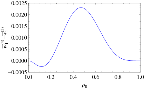
Figure 4: Discrepancy between the steady-state expectation $\bar{w}_{1}=\left\langle\sigma_{i}\sigma_{i+1}\sigma_{i+2}\sigma_{i+3}\right\rangle$ calculated with the $4$-site ($w^{(4)}_{1}$) and the $3$-site ($w^{(3)}_{1}$) approximations.

3.4.3 Probability of clusters of length $m$.

The procedure here is identical to that applied for the $3$-site approximation, namely, decompose $P_{m+2}\left(1-\sigma,\sigma,\ldots,\sigma,1-\sigma\right)$ with $\sigma=0,1$ in term of the elementary 4-site probabilities. The new element is that clusters of length $m=2$ can now be described directly by these elementary probabilities, $P^{(4)}_{cl}\left(\rho_{0},2\right)=y_{3}+y_{4}$ [see Eq. (48)] and yield

$$P^{(4)}_{cl}\left(\rho_{0},2\right)=\bar{y}\left(\rho_{0}\right)\left[\rho_{0}e^{-\bar{G}\left(1-\rho_{0}\right)}+\left(1-\rho_{0}\right)e^{-\bar{G}\left(\rho_{0}\right)}\right].$$ (56bycacd)

The probability of clusters of length $m>2$ is given by

$$P^{(4)}_{cl}\left(\rho_{0},m\right)=\frac{\left(\bar{\psi}-\bar{w}_{1}\right)^{2}}{\bar{\psi}}\left(\frac{\bar{w}_{1}}{\bar{\psi}}\right)^{m-3}+\frac{\left(\bar{\psi}_{-1}-\bar{w}_{-1}\right)^{2}}{\bar{\psi}_{-1}}\left(\frac{\bar{w}_{-1}}{\bar{\psi}_{-1}}\right)^{m-3}$$ (56bycace)

where $\bar{\psi}_{-1}\left(\rho_{0}\right)=\bar{\psi}\left(1-\rho_{0}\right)$ and $\bar{w}_{-1}\left(\rho_{0}\right)=\bar{w}_{1}\left(1-\rho_{0}\right)$ with $\bar{\psi}$ and $\bar{w}_{1}$ given by Eqs.  (35) and (56bycacc), respectively. These probability distributions are exhibited in Figs. 5 and 6. We find a perfect fitting of the simulation data for $m=2$; for $m>2$ the fitting is good but there are discrepancies in the vicinity of $\rho_{0}=0.5$, which are not perceptible in the scale of the figures.

3.4.4 Two-site correlations.

Since the results of the $4$-site approximation reduces to those of the $3$-site for expectations involving up to three contiguous sites, correlations such as $\textrm{corr}\left(\sigma_{i},\sigma_{i+1}\right)$ and $\textrm{corr}\left(\sigma_{i},\sigma_{i+2}\right)$ are the same as for the $3$-site approximation. In addition $\left\langle\sigma_{i}\sigma_{i+3}\right\rangle_{\left(4\right)}=w_{1}+y_{3}$ and so

$$\left\langle\sigma_{i}\sigma_{i+3}\right\rangle_{\left(4\right)}=\bar{\rho}\left(\rho_{0}\right)+\bar{y}\left(\rho_{0}\right)\left[\left(1-\rho_{0}\right)e^{-\bar{G}\left(\rho_{0}\right)}+\rho_{0}e^{-\bar{G}\left(1-\rho_{0}\right)}-3\right].$$ (56bycacf)

However, we need the decomposition in terms of the elementary 4-site probabilities to calculate expectations involving more distant sites, such as

$$\left\langle\sigma_{i}\sigma_{i+4}\right\rangle_{\left(4\right)}=\frac{\bar{w}_{1}^{2}}{\bar{\psi}}+\frac{\left(\bar{\psi}_{-1}-\bar{w}_{-1}\right)^{2}}{\bar{\psi}_{-1}}+2\rho_{0}\bar{y}\left(\rho_{0}\right)e^{-\bar{G}\left(1-\rho_{0}\right)}.$$ (56bycacg)

These correlations are shown in Figs. 7. Following the already observed pattern, we find a perfect agreement with the simulation data for quantities whose calculation involves expectations of up to 4 contiguous sites.

4 Discussion

Although the main purpose of this contribution is to show the remarkably good predictions of the $3$ and $4$-site approximations to describe the steady-state properties of the extended one-dimensional majority-vote model, here we focus on the discussion of those properties rather than on the procedure to derive them.

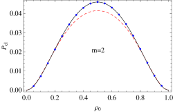
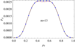
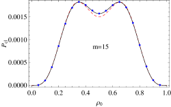
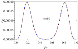
Figure 5: (Color online) Probability of finding clusters of length $m=2,13,15$ and $50$ as indicated in the figures. The dashed curves are the results of the $3$-site approximation and the solid curves of the $4$-site approximation. The filled circles are the simulation data for a ring of size $L=10^{4}$ and $10^{6}$ independent samples; the error bars are smaller than the symbol sizes. The transition from a unimodal to a bimodal distribution takes place at $m=13$.

Figure 5 presents the probability of an absorbing configuration exhibiting a cluster of length $m$ as function of the fraction of $1$s in the random initial configuration. The $3$-site approximation does not provide a good quantitative account of the simulation data but it does provide an excellent qualitative picture which captures the change of $P_{cl}$ from unimodal to bimodal that takes place for $m=13$. As for the $4$-site approximation, it provides a very good quantitative representation of the simulation data. In fact, the fitting is perfect for $m=2$ only, but the discrepancies are so small for $m>2$ that they are barely visible in the scale of the figure. We note that the transition of the distribution $P_{cl}\left(\rho_{0},m\right)$ from unimodal to bimodal was expected. In fact, long clusters should be abundant for initial configurations with $\rho_{0}$ close to $1$ or $0$ and very rare when the number of 1s and 0s is well balanced as for $\rho_{0}=0.5$. What is surprising is that the transition occurs for relatively large $m$, indicating, for example, that it is more likely to find clusters of length 10 by starting with a balanced initial configuration than with an unbalanced one. Our simulations indicate that the transition from unimodal to bimodal takes place at $m=13$ already for $L>17$. In addition, the distribution of cluster lengths is unimodal for $L\leq 9$ for all $2\leq m\leq L-2$.

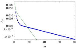
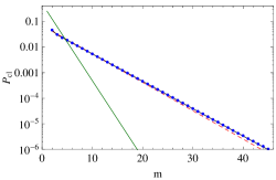
Figure 6: (Color online) Probability of finding clusters of length $m$ for fixed $\rho_{0}=0.2$ (left panel) and $\rho_{0}=0.5$ (right panel). The $3$-site approximation (dashed curves) and $4$-site approximations (solid lines connecting the symbols) give results which are indistinguishable from the simulation data (filled circles) in the scale of the figure for $\rho_{0}=0.2$; only for very large clusters one can see a noticeable discrepancy between the data and the results of the $3$-site approximation for $\rho_{0}=0.5$. For the purpose of comparison, the solid curves exhibit the results for randomly assembled configurations. The simulations were carried out for a ring of size $L=10^{4}$ and $10^{6}$ independent samples.

Figure 6 shows the dependence of $P_{cl}\left(\rho_{0},m\right)$ on $m$ for fixed $\rho_{0}$. It is not possible to distinguish from the results of the $3$ and $4$-site approximations and the simulation data for $\rho_{0}=0.2$ but some observable discrepancies appear between the $3$-site approximation and the data for large $m$ in the case $\rho_{0}=0.5$. The distribution is given by the sum of two exponentials [see Eqs.  (38) and (56bycace)] that account for the different possibilities of occurrence associated to clusters composed of 1s and 0s for $\rho_{0}\neq 0.5$. For $\rho_{0}=0.5$ the arguments of the two exponentials become identical and so we have a single exponential decay. Clearly, for $\rho_{0}=0.2$ clusters composed of 1s are dominant for small $m$ whereas clusters of 0s dominate in the large $m$ regime. The slopes of the exponentials are complicated functions of $\rho_{0}$, which can be well-approximated by Eq. (56bycace) derived within the $4$-site approximation scheme. For comparison, Fig. 6 shows $P_{cl}$ for randomly assembled configurations which is given by

$$P^{random}_{cl}\left(\rho_{0},m\right)=\left(1-\rho_{0}\right)^{2}\rho_{0}^{m}+\rho_{0}^{2}\left(1-\rho_{0}\right)^{m}.$$ (56bycach)

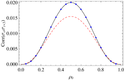
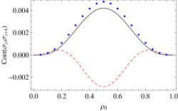
Figure 7: (Color online) Comparison of the results for the 2-site correlations obtained with the $3$-site approximation (dashed curves), the $4$-site approximation (solid curve) and the simulations (filled circles). The error bars are smaller than the symbol sizes. The left panel exhibits $\textrm{corr}\left(\sigma_{i},\sigma_{i+3}\right)$ for which the $4$-site approximation matches the data perfectly, and the right panel shows $\textrm{corr}\left(\sigma_{i},\sigma_{i+4}\right)$ where we can see the failure of that approximation scheme. The simulations were carried out for a ring of size $L=10^{4}$ and $10^{6}$ independent samples.

The failure of the $4$-site approximation in describing all the steady-state properties of the extended majority-vote model is better appreciated when we consider the 2-site correlations, as shown in Fig.7. As already pointed out, the correlations $\textrm{corr}\left(\sigma_{i},\sigma_{i}\right)$, $\textrm{corr}\left(\sigma_{i},\sigma_{i+1}\right)$ and $\textrm{corr}\left(\sigma_{i},\sigma_{i+2}\right)$ are described perfectly by both the 3 and 4-site approximations since they involve expectations of two and three contiguous sites only, so Fig. 7 exhibits the more challenging correlations, $\textrm{corr}\left(\sigma_{i},\sigma_{i+3}\right)$ (left panel) and $\textrm{corr}\left(\sigma_{i},\sigma_{i+4}\right)$ (right panel). The $4$-site approximation describes perfectly the former correlation but not the latter, whereas the $3$-site approximation fails in both cases. It is interesting that in all cases the 2-site correlations exhibit a peak at $\rho_{0}=0.5$. This can be explained by noting that the dynamics takes longer to freeze into one of the absorbing configurations for the well-balanced initial conditions which results in highly correlated sites. On the other hand, for $\rho_{0}$ close to its extreme values, most sites are already part of frozen random clusters formed during the assemblage of the initial configuration and so most of the sites at the final configuration are uncorrelated.

Figure 7 shows, in addition, that the quality of the approximation improves with increasing $n$, as expected. For example, estimation of $\textrm{corr}\left(\sigma_{i},\sigma_{i+4}\right)$ using the 3-site approximation (dashed curve) yields disastrous results, but the results obtained with the 4-site approximation (solid curve) are reasonable. We note that as $n$ increases the estimation of statistical measures involving $n+1$ sites is improved. In fact, the relative error resulting from use of the 3-site approximation to estimate $\textrm{corr}\left(\sigma_{i},\sigma_{i+3}\right)$ at $\rho_{0}=0.5$ is 22.5% whereas the error due to use of the 4-site approximation to estimate $\textrm{corr}\left(\sigma_{i},\sigma_{i+4}\right)$ is 11.5% only.

5 Conclusion

The extended one-dimensional majority-vote model is perhaps the simplest lattice model to exhibit an infinity of absorbing configurations. This strong ergodicity breaking is probably the reason that the model is not exactly solvable [27, 28]. From the mean-field theory perspective, which was the main focus of our paper, the nontrivial nature of the steady state of the model presented a most stimulating challenge as the usual fixed-point equations proved quite uninformative. In fact, the solution to the problem is a one-to-one mapping between the randomly assembled initial configurations, which are described statistically by the density $\rho_{0}$ of sites in state 1, and the absorbing configurations. That mapping was obtained directly in the case of the pair approximation but in the case of the $3$ and $4$-site approximations we had to solve analytically the dynamics for arbitrary $t$ and then take the asymptotic limit $t\to\infty$ in order to extract the mapping between the initial conditions and the steady state.

Although the pair approximation describes qualitatively the mapping between $\rho_{0}$ and the statistical properties of the steady state, its predictions regarding expectations involving two or more contiguous sites are not corroborated by the simulation results (see Fig. 2). The 3-site approximation, however, produces a remarkable good fitting of the simulation data for all quantities involving the expectation of three contiguous sites. Moreover, the predictions of the $4$-site approximation reduce to those of the $3$-site in the case of three contiguous sites expectations. We see this as a strong indication that the expectations $\left\langle\sigma_{i}\right\rangle$, $\left\langle\sigma_{i}\sigma_{i+2}\right\rangle$ and $\left\langle\sigma_{i}\sigma_{i+2}\sigma_{i+3}\right\rangle$ given by Eqs. (24), (34) and (35) are exact results. In addition, the perfect fitting of the simulation data by the expectation $\left\langle\sigma_{i}\sigma_{i+2}\sigma_{i+3}\sigma_{i+4}\right\rangle$, calculated within the $4$-site approximation [see Eq. (56bycacc)] indicates that this quantity may be exact as well, but this evidence is not so strong as for the 3-site expectations.

The findings summarized above as well as a purely numerical analysis of the $5$ and $6$-site approximations (data not shown) reveal a most remarkable pattern: the $n$-site approximation seems to yield the exact results for steady-state expectations involving $n$ contiguous sites for $n>2$. We hope our paper will motivate further research to prove (or disprove) this assertion.

References

References

- [1] Hopfield J J, Neural networks and physical systems with emergent collective computational abilities 1982 Proc. Natl. Acad. Sci. USA 79 2554
- [2] Stein D L and Anderson P W, A model for the origin of biological catalysis 1984 Proc. Natl. Acad. Sci. USA 81 1751
- [3] de Oliveira, V M and Fontanari J F, Complementarity and Diversity in a Soluble Model Ecosystem 2002 Phys. Rev. Lett. 89 148101
- [4] Lewenstein M, Nowak A and Latané B, Statistical mechanics of social impact 1992 Phys. Rev. A 45 763
- [5] Mézard M, Parisi, G and Virasoro M A 1987 Spin Glass Theory and Beyond (Singapore: World Scientific)
- [6] Castellano C, Fortunato S, and Loreto V, Statistical physics of social dynamics 2009 Rev. Mod. Phys. 81 591
- [7] Axelrod R, The Dissemination of Culture: A Model with Local Convergence and Global Polarization 1997 J. Conflict Res. 41 203
- [8] Castellano C, Marsili M, and Vespignani A, Nonequilibrium Phase Transition in a Model for Social Influence 2000 Phys. Rev. Lett. 85 3536
- [9] Vilone D, Vespignani A and Castellano C, Ordering phase transition in the one-dimensional Axelrod model 2002 Eur. Phys. J. B 30, 399
- [10] Barbosa L A and Fontanari J F, Culture-area relation in Axelrod’s model for culture dissemination 2009 Theory Biosci. 128 205
- [11] Ligget T M 1985 Interacting Particle Systems (New York: Springer)
- [12] Gray L 1985 Particle Systems, Random Media, and Large Deviations (Providence, RI: American Mathematical Society) Vol. 41, pp. 149–160.
- [13] Parisi D, Cecconi F and Natale F, Cultural Change in Spatial Environments 2003 J. Conflict Res. 47 163
- [14] Peres L R and Fontanari J F, Statistics of opinion domains of the majority-vote model on a square lattice 2010 Phys. Rev. E 82 046103
- [15] Krapivsky P L, Kinetics of monomer-monomer surface catalytic reactions 1992 Phys. Rev. A 45 1067
- [16] Krapivsky P L and Redner S, Dynamics of Majority Rule in Two-State Interacting Spin Systems 2003 Phys. Rev. Lett. 90 238701
- [17] Galam S, Heterogeneous beliefs, segregation, and extremism in the making of public opinions 2005 Phys. Rev. E 71 046123
- [18] Lambiotte R and Redner S, Dynamics of non-conservative voters 2008 EPL 82 18007
- [19] Boyd R and Richerson P J 1985 Culture and the Evolutionary Process (Chicago: University of Chicago Press)
- [20] Tomé T, de Oliveira M J, and Santos M A, Non-equilibrium Ising model with competing Glauber dynamics 1991 J. Phys. A 24 3677
- [21] de Oliveira M J, Isotropic majority-vote model on a square lattice 1992 J. Stat. Phys. 66 273
- [22] Konno N and Katori M, Applications of the CAM Based on a New Decoupling Procedure of Correlation Functions in the One-Dimensional Contact Process 1990 J. Phys. Soc. Jpn. 59 1581
- [23] ben-Avraham D and Köhler J, Mean-field -cluster approximation for lattice models 1992 Phys. Rev. A 45 8358
- [24] Ferreira A L C and Mendiratta S K, Mean-field approximation with coherent anomaly method for a non-equilibrium model 1993 J. Phys. A 26 L145
- [25] Ferreira A A and Fontanari J F, The -site approximation for the triplet-creation model 2009 J. Phys. A 42 085004
- [26] Ince E L 1956 Ordinary Differential Equations (New York: Dover Publications)
- [27] Privman V 1997 Nonequilibrium Statistical Mechanics in One Dimension (Cambridge, UK: Cambridge University Press)
- [28] Marro J and Dickman R 1999 Nonequilibrium Phase Transitions in Lattice Models (Cambridge, UK: Cambridge University Press)