Radiative annihilation of a soliton and an antisoliton in the coupled sine-Gordon equation

Abstract

In the sine-Gordon equation solitons and antisolitons in the absence of perturbations do not annihilate. Here I present numerical analysis of soliton-antisoliton collisions in the coupled sine-Gordon equation. It is shown that in such a system soliton-antisoliton pairs (breathers) do annihilate even in the absence of perturbations. The annihilation occurs via a logarithmic-in-time decay of a breather caused by emission of plasma waves in every period of breather oscillations. This also leads to a significant coupling between breathers and propagating waves, which may lead to self-oscillations at the geometrical resonance conditions in a dc-driven system. The phenomenon may be useful for achieving superradiant emission from coupled oscillators.

I Introduction

Analysis of soliton dynamics in the sine-Gordon (SG) formalism is important in many research areas Kivsh_Malomed_RMP , including non-linear optics, condensed matter physics, atomic Braun and particle physics QuantumSG . Solitons are elementary particles of the sine-Gordon equation, in a sense that they are quantized and do not spontaneously decay. Soliton-antisoliton collision is a nontrivial example of interaction of strongly non-linear waves. It may lead either to passage of the two waves or to formation of a bound pair - the breather Scott . Within the pure SG equation soliton and antisoliton do not annihilate because the collision is elastic and the annihilation is prohibited by energy conservation. However, addition of various perturbation terms to the SG equation does allow particle-antiparticle annihilation via breather decay Scott ; PedersenAnnih . This may happen both via intrinsic viscous damping and via radiative losses from the breather Kivsh_Malomed_RMP .

In recent years properties of solitons in the coupled sine-Gordon equation (CSGE) are being actively studied. The CSGE describes complex behavior of interacting systems, such as atoms in a periodic potential Braun , magnetic multilayers MagneticML , stacked Josephson junctions SBP ; SakUstFiske ; Modes ; Fluxon and layered superconductors KleinerMuller94 ; KatterweFrau ; KatterweFiske . Coupling of $N$ systems leads to a variety of unusual effects. First of all, it leads to appearance of $N$ eigenmodes with different symmetries, length scales and velocities KleinerModes ; SakUstFiske . Even though the exact soliton solution in this case is not known, numerical and approximate analytic results demonstrated that the soliton becomes composed of different eigenmodes Modes ; Fluxon and the shape of such a composite soliton may become very unusual in the dynamic case. Next, unlike the sine-Gordon equation, the coupled sine-Gordon equation is not Lorentz-invariant KatterweFiske . Therefore superluminal soliton motion (faster than the slowest eigenmode velocity) is possible Modes ; Cherenkov ; KatterweFiske . It is accompanied by Cherenkov-type radiation, due to decomposition of soliton components with eigenmode velocities slower than the speed of the soliton into plasma waves travelling along with the soliton Modes ; Fluxon ; Cherenkov .

In this work I present numerical analysis of soliton-antisoliton collisions within the coupled sine-Gordon equation with focus on Josephson vortex (fluxon) dynamics in magnetically coupled stacked Josephson junctions. Both direct (fluxon and antifluxon in the same junction) and indirect (fluxon and antifluxon in different junctions) collisions are considered. It is demonstrated that soliton-antisoliton pair in the CSGE can annihilate even in the absence of viscous damping or other perturbations. Annihilation occurs via emission of plasma waves from an oscillating breather, to some extent resembling annihilation of elementary particles via emission of a pair of photons. The radiative annihilation leads to a significant coupling of a breather to linear waves and brings about a variety of resonant and self-oscillation phenomena Breather , which can be useful for achieving a coherent superradiant emission from coupled systems Ozyuzer ; Breather .

II General relations

We consider one-dimensional chains/junctions described by the perturbed sine-Gordon equation:

$$\varphi^{\prime\prime}-\ddot{\varphi}-\alpha\dot{\varphi}=\sin\varphi-\gamma,$$ (1)

where $\varphi$ is the phase variables, “primes” and “dots” denote spatial $\varphi^{\prime}=\partial\varphi/\partial x$ and temporal $\dot{\varphi}=\partial\varphi/\partial t$ derivatives, $\alpha$ is the viscous damping parameter and $\gamma$ is the driving (bias) term. In the absence of perturbation terms $\alpha=\gamma=0$ it reduces to the pure SG equation:

$$\varphi^{\prime\prime}-\ddot{\varphi}=\sin\varphi.$$ (2)

The soliton in the SG Eq.(2) is a $2\pi$ phase kink Scott :

$$F=4\arctan[\exp(x-ut)/\sqrt{1-u^{2}}],$$ (3)

where $u$ is the velocity of the soliton, normalized by the speed of light (the Swihart velocity). The velocity dependent factor represents the relativistic contraction of the soliton when its velocity approaches the speed of light $u\rightarrow 1$ Scott . This is the consequence of Lorentz invariance of the SG equation (2). The normalized energy of a static soliton $u=0$ is $E_{sol}=8$.

II.1 The coupled sine-Gordon equation

We assume that a system of $N$ interacting junctions can be described by the perturbed CSGE SBP :

$$\varphi_{i}^{\prime\prime}={\bf A_{ij}}\left[\ddot{\varphi}_{j}+\alpha\dot{\varphi}_{j}+\sin\varphi_{j}-\gamma\right].$$ (4)

Here $i,j=1,2,...N$ is the junction index and ${\bf A}_{ij}$ is the coupling matrix, off-diagonal elements of which describe interaction between different junctions. In what follows we will consider the simplest case of nearest neighbor interaction, described by a symmetric tridiagonal matrix the only nonzero elements of which are:

$A_{i,i}=1,~{}A_{i,i-1}=A_{i,i+1}=-S$.

Here $S<0.5$ is the coupling strength. The CSGE can be also written in the equivalent inverted form

$${\bf A_{ij}^{-1}}\varphi_{i}^{\prime\prime}-\ddot{\varphi}_{j}-\alpha\dot{\varphi}_{j}=\sin\varphi_{j}-\gamma.$$ (5)

Apparently, for $N=1$ it reduces to the perturbed SG Eq. (1). In case of two coupled chains $N=2$, the system of unperturbed CSGE $\alpha=\gamma=0$ reads:

$$\frac{1}{1-S^{2}}\varphi_{1}^{\prime\prime}-\ddot{\varphi}_{1}=\sin\varphi_{1}-\frac{S}{1-S^{2}}\varphi_{2}^{\prime\prime},$$ (6)

$$\frac{2}{1-S^{2}}\varphi_{1}^{\prime\prime}-\ddot{\varphi}_{2}=\sin\varphi_{2}-\frac{S}{1-S^{2}}\varphi_{1}^{\prime\prime}.$$ (7)

It is easy to verify by direct application of the Lorentz transformation that the CSGE is not Lorentz invariant, unlike the SG equation (2).

Physically, the considered type of coupling corresponds e.g., to magnetic (inductive) interaction of stacked Josephson junctions SBP . In this case space and time in the dimensionless equations are normalized by the Josephson penetration depth, $\lambda_{J}$, and the Josephson plasma frequency $\omega_{p}$, respectively, the velocity is normalized by the Swihart velocity $c_{0}=\lambda_{J}\omega_{p}$ and $\gamma$ by the Josephson critical current $\gamma=I/I_{c}$. More details on the normalization and the formalism can be found in Refs.Modes ; Fluxon . As mentioned in the introduction, coupling terms as in Eqs. (4,5) are also relevant for other objects, like atomic chains Braun and magnetic multilayers MagneticML .

The energy density of the coupled system is Modes ; Fluxon

$$\frac{\partial E(x)}{\partial x}=\frac{1}{2}\varphi_{j}^{\prime}{\bf A_{ij}^{-1}}\varphi_{i}^{\prime}+\sum_{i=1}^{N}(1-\cos\varphi_{i})+\frac{1}{2}\dot{\varphi}_{i}^{2}.$$ (8)

Here the first, the second and the third terms represent correspondingly the magnetic/elastic, the Josephson/potential and the electric/kinetic energies for the case of a junction/chain.

Coupling leads to splitting of the dispersion relation of small oscillations into $N$ eigenmodes with different symmetries and propagation velocities KleinerModes ; SakUstFiske :

$$c_{n}=\left[1-2S\cos\frac{\pi n}{N+1}\right]^{-1/2},~{}(n=1,2,...,N).$$ (9)

The slowest mode $n=N$ corresponds to out-of-phase (antisymmetric) oscillations in neighbor junctions and the fastest, $n=1$ to the in-phase (symmetric) oscillations in all the junctions Note1 .

II.2 A single soliton in the unperturbed CSGE

For the solitonic motion with a constant velocity $u$, $\varphi(x,t)=\varphi(x-ut)$, the unperturbed CSGE Eq. (5) with $\alpha=\gamma=0$ can be written in the simple vector form Fluxon :

$$[{\bf A_{ij}^{-1}}-u^{2}{\bf E}]{\bf\varphi}^{\prime\prime}=\sin{\bf\varphi}.$$ (10)

Here ${\bf E}$ is the unitary matrix. This equation is essentially similar to the static CSGE, for which the first integral is known Modes . Therefore we can in a similar manner write the first integral for the solitonic motion:

$$\frac{1}{2}\varphi_{j}^{\prime}[{\bf A_{ij}^{-1}}-u^{2}{\bf E}]\varphi_{i}^{\prime}-\Sigma_{i=1}^{N}[1-\cos\varphi_{i}]=C.$$ (11)

For a single soliton the constant $C=0$ because at the infinity $\varphi_{i}=\varphi_{i}^{\prime}=0$. From comparison with the general expression for the energy density Eq. (8), it is easily seen that the soliton energy is twice the magnetic/elastic energy

$$E_{sol}=2E_{m}=\int dx\varphi_{j}^{\prime}{\bf A_{ij}^{-1}}\varphi_{i}^{\prime},$$ (12)

as is also the case for the soliton in the SG equation Scott .

The exact soliton solution in the CSGE is not yet known. However, an approximate composite soliton solution has been proposed, verified by numerical simulations and by perturbation correction calculations Modes ; Fluxon . It is represented by a linear superposition of solitonic waves Eq. (3), corresponding to different eigenmodes.

$$\varphi_{i}\simeq\sum_{n=1}^{N}\kappa_{n,i}F_{n},~{}(i=1,2,...,N),$$ (13)

$$F_{n}=4\arctan\left[\exp\left(\frac{x-ut}{\lambda_{n}\sqrt{1-u^{2}/c_{n}^{2}}}\right)\right].$$ (14)

Here $i$ is the junction number, $\lambda_{n}$ is the characteristic length scale of the eigenmode $n$:

$$\lambda_{n}=\left[1-2S\cos\frac{\pi n}{N+1}\right]^{-1/2},~{}(n=1,2,...,N).$$ (15)

Note that $\lambda_{n}^{-2}$ are eigenvalues of the coupling matrix ${\bf A_{ij}}$ and coefficients $\kappa_{n,i}$ are components of the eigenvectors of ${\bf A_{ij}}$, normalized so that $\sum_{n=1}^{N}\kappa_{n,i}=1$ in the junction containing the soliton and zero in all other junctions Fluxon ; Note1 . Thus the soliton consists of a $2\pi$ kink in one junction and ripples in all other junctions. The soliton shape (coefficients $\kappa_{n,i}$) does depend on the junctions number and is, for example, different for the soliton in the outmost and in the central junctions of the stack. Amplitudes of ripples in the neighbor junctions depend on the coupling strength and can be significant in the strong coupling case $S\simeq 0.5$. The ripples decrease with the distance from the soliton both along and across the junctions.

As discussed in Ref. Modes , the static soliton energy in the CSGE is larger than that in the single SG equation both due to presence of ripples in neighbor chains and reconstruction of characteristic length scales Eq.(15). Let’s, for example, estimate the energy in the simplest case $N=2$. In this case the multicomponent soliton, Eq. (13), becomes Note1

$$N=2:\left\{\begin{array}[]{c}\varphi_{1}=\frac{F_{1}+F_{2}}{2},~{}\lambda_{1}=\left(1-S\right)^{-1/2}\\ \varphi_{2}=\frac{F_{1}-F_{2}}{2},~{}\lambda_{2}=\left(1+S\right)^{-1/2}\end{array}\right.$$ (16)

Substituting those into Eq. (12) and taking into account that $A_{1,1}^{-1}=A_{2,2}^{-1}=1/(1-S^{2})$ and $A_{1,2}^{-1}=A_{2,1}^{-1}=S/(1-S^{2})$ we obtain

$$\begin{array}[]{c}E_{sol}(N=2)=\frac{2}{1-S^{2}}\left[\lambda_{1}^{-1}(1+S)+\lambda_{2}^{-1}(1-S)\right]=\\ 4[(1+S)^{-1/2}+(1-S)^{-1/2}].\end{array}$$ (17)

For $S=0.5$ we get $E_{sol}(N=2)\simeq 8.92$, which is $\simeq 1.12$ times larger than $E_{sol}(N=1)=8$ for a single junction, in good agreement with numerical simulations Modes . The soliton energy increases with $N$ and saturates at $\simeq 3.6E_{sol}(N=1)$ in the strong coupling case $S=0.5$ CommentFl .

The shape of the soliton in the CSGE experiences strong metamorphoses in the dynamic case Modes ; Fluxon . Indeed, since the soliton components $F_{n}$, Eq. (13), experience Lorentz contraction at different characteristic velocities $c_{n}$, Eq. (9), the relative shape of the soliton does not remain the same as in the static case. When $u$ approaches the slowest velocity $c_{N}$, the corresponding component $n=N$ gets contracted, while the rest of the soliton remains uncontracted. Such the partial Lorentz contraction was confirmed by numerical simulations Modes ; Fluxon . The soliton survives even at superluminal velocity $u>c_{N}$, however in this case the characteristic length $\lambda_{N}$ becomes imaginary due to the Lorentz factor. This corresponds to transformation of the corresponding soliton component $F_{N}$ into the out-of-phase plasma wave Modes . A similar process of decomposition of soliton components into plasma waves with corresponding symmetries occurs when $u$ exceeds any of the characteristic velocities $c_{n}$ Fluxon . The phenomenon resembles Cherenkov emission from a superluminal particle Modes ; Cherenkov ; Fluxon with the exception that the speed of light is multiple-valued, Eq. (9), and the dispersion relation is different.

Multisoliton states in the CSGE are dominated by a profound metastability Modes ; Compar ; KatterweFrau , i.e., for given boundary conditions a large variety of metastable soliton distributions is possible. Moving solitons interact with linear waves, which leads to appearance of geometrical resonances (standing waves) in finite size systems. Note that a soliton in the CSGE can excite all eigenmodes Eq.(9), which leads to a large variety of geometrical resonances SakUstFiske ; KatterweFiske .

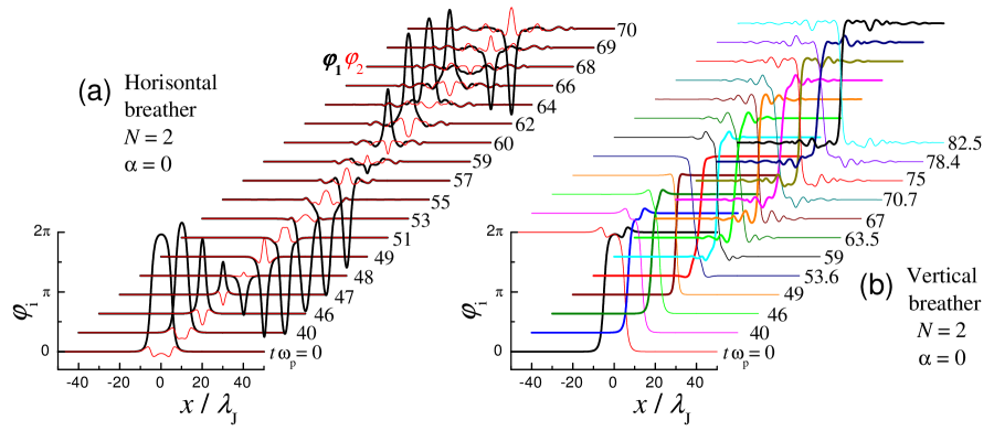
Figure 1: (Color online). Snapshots of time evolution of phase distributions upon soliton-antisoliton collision in the unperturbed ($\alpha=\gamma=0$) double-junction CSGE for (a) direct collision of a solton and an antisoliton in the junction-1 and (b) indirect collision of a soliton in the junction-1 and an antisoliton in the junction-2. Thick and thin lines represent $\varphi_{1}$ and $\varphi_{2}$, respectively. It is seen that both the horizontal (a) and vertical (b) breathers are decaying due to emission of plasma waves, even in the absence of perturbations.

II.3 Breathers

Breather is a bound soliton-antisoliton pair. The breather solution of the SG equation Eq. (2) in the center-of-mass frame is Scott

$$\varphi=4\arctan\left(\frac{\tan\nu\sin[(\cos\nu)t]}{\cosh[(\sin\nu)x]}\right).$$ (18)

Here $0<\nu<\pi/2$ is determining the breather amplitude $\varphi_{Br}=4\nu$. The breather is oscillating without annihilation or decay at a frequency $\omega_{Br}=\cos\nu$, which is always less than the plasma frequency $\omega_{Br}<1$. The solution Eq. (18) is valid for an infinite system $L=\infty$. A more complicated solution for the finite size system can be found in Ref. Costabile . The total energy of the breather $E_{Br}=16\sin\nu$ is smaller than the energy of two static solitons $E_{Br}<2E_{sol}=16$, leading to binding of the soliton and the antisoliton.

Finite dissipation $\alpha>0$ leads to decay of the breather and facilitates soliton-antisoliton annihilation. The decay is primarily caused by the viscous damping of the soliton-antisoliton motion. However, minor radiative losses also appear Kivsh_Malomed_RMP . A qualitative change of the wave form takes place upon the soliton-antisoliton annihilation. Initially, the soliton-antisoliton pair ($4\nu\simeq 2\pi$) shrinks, i.e., the maximum separation between the pair $\Delta x\sim 1/\tan\nu\gg 1$ gradually decreases after every collision. At $4\nu\lesssim\pi$, the soliton and the antisoliton completely merge and can no longer be distinguished. Further decay (reduction of $\nu$) leads to expansion of the breather. From Eq. (18) it follows that for small $\nu\ll 1$ the size of the breather is $\propto 1/\sin\nu$. Eventually, the breather turns into the longitudinal plasma wave with $\omega_{Br}=\cos\nu\simeq 1$ and the wave number $k_{x}\simeq\sin\nu\simeq 0$. This accomplishes the soliton-antisoliton annihilation.

Breathers play role not only in soliton-antisoliton annihilation and the opposite (time-reversal) process of creation (or penetration) of the soliton CommentFl . Breathers also interact with traveling waves and external forces Kivsh_Malomed_RMP . In Ref. Breather it was argued that breathers in the CSGE can help to pump energy from the external dc-power supply ($\gamma$ term in Eq. (4)) into the oscillating travelling waves, which leads to appearance of self-oscillations in the dc-driven CSGE with $\gamma>0$. The phenomenon may find practical applications for generation of coherent (superradiant) THz sources based on stacked intrinsic Josephson junctions in high-temperature superconductors Ozyuzer .

In the CSGE we will consider two distinctly different types of breathers (referred to as the horizonal and the vertical):

(i) the ”horizontal” breather corresponds to a direct collision of a soliton and an antisoliton in the same junction.

(ii) the ”vertical” breather corresponds to an indirect collision of a soliton and an antisoliton in different junctions. Unlike the horizontal breather, the vertical breather does not annihilate even in the presence of dissipation, but leads to formation of a stable static soliton-antisoliton pair Compar ; KleinerAntiFlux . For $N=2$ the static ”vertical” soliton-antisoliton pair has an exact antisymmetric solution SBP : $\varphi_{1}=-\varphi_{2}=F_{2}$. The energy of the vertical pair

$$E_{vert}(N=2)=2\times 8\lambda_{2}^{-1}=16(1+S)^{-1/2}$$ (19)

is smaller than twice the isolated soliton energy Eq.(17), leading to binding of the pair.

II.4 Numerical procedure

The system of partial differential equations Eq.(5) for different $N$ and junction length $L$ is solved numerically using an explicit finite difference method (central difference in space and time). The spatial mesh size $\Delta x$ was typically 0.025 and the temporal $\Delta t=\Delta x/10$. The absence of spurious effects was checked by changing mesh sizes and integration times.

Static solitons and antisolitons Eq. (3) were introduced at certain positions at the initial time. The system is then given long enough time to relax with a large damping factor $\alpha=2$. The large viscosity prevents significant soliton motion during the transient period. After that calculations continued with the desired value of $\alpha$. The time count $t=0$ starts from the end of the transient period.

All simulations were made for zero external field boundary conditions at $x=\pm L/2$

$$\partial\varphi_{i}/\partial x=0.$$ (20)

Those boundary conditions are non-radiative, i.e., preclude energy flow through the edges Hu . In some cases dynamic radiative boundary conditions were employed (still at zero external field) following Ref. TheoryFiske . The radiation emission is facilitated by the finite radiation impedance $Z$. For more details see Ref. TheoryFiske .

All presented simulations are done for the strong coupling case $S\simeq 0.5$, close to the maximum value, relevant e.g. for atomic scale intrinsic Josephson junctions KleinerMuller94 ; Fluxon ; KatterweFiske ; KatterweFrau . It was checked that variation of the coupling strength does not affect the qualitative presence of the effects described below.

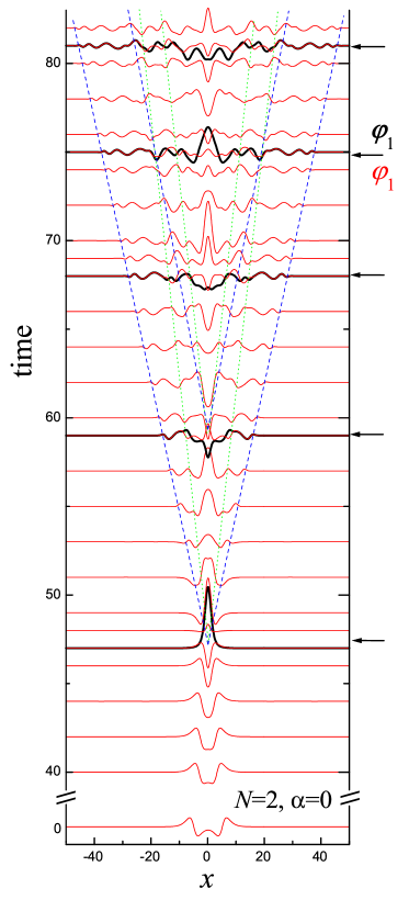
Figure 2: (Color online). Detailed view of the time evolution of $\varphi_{2}$ (thin lines) for the horizontal breather from Fig. 1 (a). The phase $\varphi_{1}$ (thick lines) is shown close to the moments of collisions, marked by arrows. It is seen that emission of two wave fronts occurs at every collision: the fast front (marked by blue dashed lines) has an in-phase symmetry $\varphi_{1}=\varphi_{2}$ and propagates with the fast velocity $c_{1}$, the slow front (marked by green dotted lines) has an out-of-phase symmetry $\varphi_{1}=-\varphi_{2}$ and propagates with the slow velocity $c_{N}$.

III Results

III.1 Unperturbed soliton-antisoliton dynamics

Figure 1 shows time sequence of calculated phase profiles $\varphi_{1}$ (thick lines) and $\varphi_{2}$ (thin lines) for the unperturbed ($\alpha=\gamma=0$) CSGE in a double junction system $N=2$, Eq. (7), for the horizontal (a) and the vertical (b) breathers. Initially at $t=0$ the soliton and the antisoliton are well separated. The solitons collide for the first time approximately at the same time ($t_{1}\simeq 47$). For a single SG equation, the breather Eq. (18) would continue to oscillate without decay with the same periodicity, i.e. the subsequent collision would occur at time intervals $2t_{1}$. This is clearly not the case in the unperturbed CSGE:

(i) First of all, subsequent collisions occur at smaller time intervals. For example, the second collision for both breather occurs at $t_{2}\simeq 59$ and $t_{2}-t_{1}\simeq 12$ much shorter than $2t_{1}\simeq 94$. The third collision for the horizontal breather occurs at $t_{3}\simeq 68$ and $t_{3}-t_{2}\simeq 9$ and so on.

(ii) Second, the amplitude of the horizonal breather decays with time. The soliton and the antisoliton in the vertical breather can not change their $\pm 2\pi$ amplitudes, instead they slow down and eventually form a static pair.

(iii) Travelling waves are emanating from the breather after the collision.

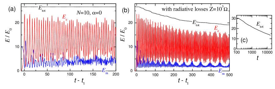
Figure 3: (Color online). Time dependence of the total $E_{tot}$, electric $E_{e}$ and magnetic $E_{m}$ energies for a horizontal breather in junction $i=5$ of the unperturbed $N=10$ CSGE system. (a) Without radiative losses at the edges $Z=\infty$, (b) with radiative losses $Z=10^{5}~{}\Omega$. Panel (c) shows a long-time evolution of $E_{tot}(t)$ in the presence of radiative losses. A peculiar logarithmic time decay is seen.

Figure 2 shows time dependence of $\varphi_{2}$ for the horizonal breather from Fig. 1 (a). For simplification the phase $\varphi_{1}$ (thick lines) is shown only at the moments of collisions, marked by arrows. It is clearly seen that waves are emitted from the breather upon the first soliton-antisoliton collision $t_{1}\simeq 47$. Two wave fronts can be distinguished: the faster (marked by the lower dashed blue lines) propagate with a constant speed $c_{1}=1.414$, and the slower (marked by the lower dotted green lines) with the speed $c_{2}=0.8165$ in agreement with Eq. (9). A comparison of $\varphi_{1,2}$ clearly demonstrates that the faster front has the in-phase $\varphi_{1}=\varphi_{2}$ and the slower the out-of-phase eigenmode symmetry. At the second collision $t_{2}\simeq 59$, two new wave fronts are emitted, marked by the upper dashed and dotted lines, originated at the second collision point ($x=0$, $t=59$). Every subsequent collision leads to a similar emission. We emphasize that this happens in the absence of dissipation $\alpha=0$. Therefore, the breather is decaying in the unperturbed CSGE entirely due to radiative losses.

Figure 3 (a) shows time dependence (counted from the first collision $t_{1}$) of the total energy $E_{tot}$ (top black line), the electric energy $E_{e}$, given by the third term in Eq. (8)(middle red line), and magnetic energy $E_{m}$, given by the first term in Eq. (8) (bottom blue line) for the case of a horizontal breather in the middle $i=5$ of $N=10$ coupled junctions with the length $L=100$. Calculations are made for the unperturbed CSGE $\alpha=\gamma=0$ and without radiation emission at the edges $Z=\infty$. It is seen that $E_{tot}$ is conserved because there are no dissipative or radiative losses. Maxima in $E_{e}$ and minima in $E_{m}$ occur upon soliton-antisoliton collisions. It is seen that the period of collisions is decreasing with time and the magnetic energy $E_{m}$, related to the breather amplitude, is rapidly decreasing after the first collision. This is similar to the $N=2$ case shown in Fig. 1 (a). At $t-t_{1}>L/c_{n}$ the emitted waves from the breather reflect back from the edges and come back to the breather. This leads to a very complicated phase pattern consisting of a breather and bouncing waves from all $N=10$ eigenmodes.

In order to avoid a complication associated with the reflection and bouncing of the emitted waves, we made simulations for the same parameters with a finite radiative impedance $Z$ TheoryFiske . In this case the waves partly transmit through the edges and leave the system. This leads to a decay of propagating waves, except for the destructively interfering out-of-phase mode $n=N$, which can not be emitted (see Ref. TheoryFiske for a discussion of emission efficiency of different eigenmodes).

Fig. 3 (b) presents the results of simulations for the same case as in (a) but with the finite radiative impedance. It is seen that initially the total energy is conserved until $t-t_{1}=L/2c_{1}\simeq 10$ when the fastest in-phase ($n=1$) wave front reaches the edges. After that the energy starts to decay due to radiative losses through the edges. At large times the decay of the breather energy $E_{tot}(t)$ slows down. Simultaneously, long period beatings in $E_{m}$ due to slow flexural oscillations of the breather become obvious.

Do the soliton and the antisoliton completely annihilate upon direct collision in the unperturbed CSGE, or do they eventually form a stable non-decaying breather? To answer this question we performed long-time calculations. In order to avoid possible radiative losses at the edges from the tail of the breather itself, we studied even longer systems. Fig. 3 (c) shows such simulations for $L=300$ and the rest of parameters the same as in panel (b). A peculiar logarithmic time decay is clearly seen:

$$E_{tot}(t)\simeq E_{tot}(0)-\beta\log(t/t_{1}),$$ (21)

where $\beta$ depends on the strength of radiative losses at the edges. Thus, unlike in the unperturbed sine-Gordon equation, in the unperturbed coupled sine-Gordon equation the soliton-antisoliton pair does annihilate upon the direct collision even in the absence of dissipation, but the annihilation takes an exponentially long time. Therefore, for all practical cases the breather would appear stable at the time of the experiment, just like the circulating current in type-II superconductors Tinkham .

The indirect soliton-antisoliton collision, shown in Fig. 1 (b), does not lead to annihilation, but to formation of a static bound pair. The vertical breather, produced upon the indirect collision decays in a similar way as the horizontal breather discussed above. The total radiative losses upon the indirect collision is the difference between the energy of two isolated solitons and the static vertical soliton-antisoliton pair. For the double junction, shown in Fig. 1 (b), those are given by Eqs. (17,19):

$$\Delta E(N=2)=8\left[(1-S)^{-1/2}-(1+S)^{-1/2}\right].$$ (22)

For $S=0.5$, as in Fig. 1 (b), about $27\%$ of the initial energy is lost into radiation.

III.2 Soliton-antisoliton dynamics in the perturbed CSGE

Addition of viscous damping $\alpha>0$ perturbation term leads to decay of the breather both in the single SG and in the CSGE. As seen from Fig. 3, reduction of the amplitude of breather oscillations is accompanied by the increment of oscillation frequency. Figure 4 shows the amplitude of the breather as a function of breather frequency for the SG ($N=1$) and the horizontal breather in the CSGE ($N=2$ and 10) with different damping $\alpha$. It is seen that in all cases the $\varphi_{Br}(\omega_{Br})$ dependence follows well the theoretical expression Eq. (18), shown by the dashed line. The scattering of points for the CSGE case is due to presence of the strong radiative field, which complicates the determination of the breather frequency and amplitude, see Fig. 3 (a).

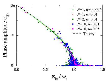
Figure 4: (Color online). Phase amplitude of the horizontal breather as a function of the breather frequency for perturbed SG ($N=1$) and CSGE with $N=2$ and 10 for different values of the damping $\alpha$ and for $\gamma=0$. The dashed line represents the breather solution Eq. (18) for the SG equation.

III.3 Collision of a driven soliton with the edge

So far we considered the case without driving force $\gamma=0$. As shown above, in the CSGE soliton and antisoliton always annihilate due to either radiative or dissipative losses. The driving force $\gamma\neq 0$ replenishes the energy lost in the collision and may lead to survival of the solitons after the collision.

In a finite system, a moving soliton will inevitably collide with the edges. For the zero-field boundary condition the collision of the soliton with the edge is equivalent to a collision with an image antisoliton Scott . After the collision the image soliton continues the motion, i.e. the soliton is reflected as an antisoliton at the edge Scott . The shuttling soliton-antisoliton motion leads to appearance of zero-field steps (ZFS) in current-voltage ($I$-$V$) characteristics of Josephson junctions PedersenAnnih ; PedersenSol ; PedersenZFS ; Binslev ; Chang . In this case, current is the dc-driving force $I=\gamma$ and dc voltage is time-average of the velocity.

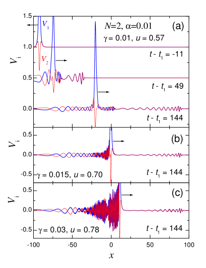
Figure 5: (Color online). Instantaneous voltage (velocity) $V(x)=\partial\varphi_{1,2}/\partial t$ profiles for a driven soliton motion in a dissipative $\alpha=0.01$ CSGE with $N=2$ for increasing driving currents (forces) (a) $\gamma=0.01$, (b) $\gamma=0.015$ and (c) $\gamma=0.03$. Time is counted with respect to the first collision $t_{1}$ with the left edge of the system. It is seen that the fast in-phase and the slow out-of-phase waves are emitted upon the collision $t=t_{1}$. In panel (b) the soliton velocity $u$ is close to the velocity of the out-of-phase wave, and the corresponding front is no longer seen ahead of the soliton. Further increase of $u$ in panel (c) leads to profound Cherenkov-type radiation behind the soliton.

Figure 5 shows snapshots of voltage profiles $V_{i}=\dot{\varphi}_{i}$ for a single soliton in the junction $i=1$ of a double junction structure $N=2$ for different driving terms $\gamma$ and for $\alpha=0.01$ and $L=200$. The time is counted relative to the first collision $t_{1}$ with the left edge. Panel (a) corresponds to a small driving force $\gamma=0.01$ and a slow, subluminal soliton motion $u=0.57<c_{N}$. Before the collision, $t-t_{1}=-11$, the soliton was moving to the left. After collision it is reflected as an antisoliton moving to the right. Simultaneously, emission of plasma waves from both the in-phase and the out-of-phase eigenmodes takes place, similar to the unperturbed case in Figs. 1 (a) and 2. Panels (b) and (c) show snapshots at larger driving forces and soliton velocities larger than the out-of-phase plasma wave speed $c_{N}$. Such superluminal soliton motion is accompanied by Cherenkov-type radiation behind the soliton Modes ; Fluxon ; Cherenkov ; Goldobin . A comparison of snapshots at $t-t_{1}=144$ in panels (a-c) indicates that the in-phase radiation front from the collision event is similar for all shown soliton velocities, but the out-of-phase front is not visible ahead of the soliton when the soliton is moving faster than the out-of-phase plasma wave Note2 . From this it is also clear that it is the edge, rather than the moving soliton, that emanates the waves.

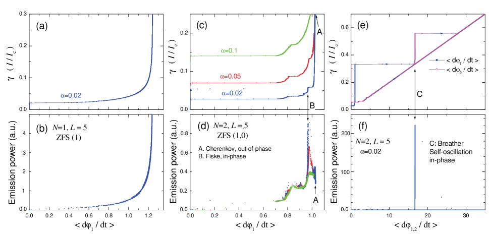
Figure 6: (Color online). Current (driving force) - Voltage (velocity) characteristics of a shuttling single soliton in a moderate size systems $L=5$ for (a) a single junction (SG, $N=1$) and (c) a double junction stack (CSGE, $N=2$), appearance of a fine structure of the zero-field step due to interference with emitted plasma waves is clearly seen. Panel (e) shows the continuation of $I-V$ characteristics at large bias for $N=2$ and $\alpha=0.02$. Panels (b), (d) and (f) show the corresponding emission powers. It is seen that in the double junction system the emission at the velocity matching part of the zero-field step (point A in (c,d)) is at minimum, unlike the single junction case (a,b), and the maximum emission occurs at point B, corresponding to the in-phase geometrical resonance and the Fiske step in the $I-V$. Above the ZFS, the system switches to another strongly emitting resonance (point C in (e,f)), which represents a breather-type self-oscillation.

III.4 Soliton resonances in finite-size systems

A shuttling soliton in a finite-size system will periodically excite travelling waves at the edges. The emanated waves also propagate along the chains and reflect back at the edges. The shuttling soliton will interact with bouncing waves. Resonance will appear if bouncing waves are in-phase with the soliton at the edges Golubov . In Josephson junctions this leads to appearance of fine structure of Zero Field Steps in $I$-$V$ characteristics Chang ; PedersenSol .

Figure 6 (c) shows calculated dc current-voltage $\gamma$ - $<\partial\varphi_{1}/\partial t>$ ($<>$ indicate averaging in time) characteristics for a moderately short $L=5$ double junction $N=2$ structure for different damping parameters $\alpha$. Calculations are made for the ZFS mode (1,0), i.e. for a single soliton shuttling in the junction $i=1$. In the second junction $<\partial\varphi_{2}/\partial t>=0$. The dc ZFS voltage is

$$V_{ZFS}(1,0)=\langle\frac{\partial\varphi_{1}}{\partial t}\rangle=\frac{2\pi u}{L}.$$ (23)

A strong almost vertical velocity-matching soliton step, marked as point A in Fig. 6 (c), occurs when the soliton velocity approaches the slowest out-of phase eigenmode velocity $u\rightarrow c_{2}$. According to Eqs. (9) and (23), for $S=0.5$, $N=2$ this occurs at $<\partial\varphi_{1}/\partial t>=1.026$. The rapid increase of the driving force $\gamma$ at $u\rightarrow c_{2}$ is caused both by a partial Lorentz contraction of the $F_{2}$ component of the composite soliton Modes and by a rapid enhancement of dissipation due to Cherenkov radiation, see Fig. 5 (b,c).

Fine structure is seen at the ZFS below the velocity matching step due to resonances between the shuttling soliton and bouncing waves emanating upon every collision of the soliton with edges. In principle, the soliton can interfere and form resonances with any type of periodically emitted waves. Those can be waves emitted by the fluxon upon passing a defect Golubov or Cherenkov-type emission Goldobin . However, the resonances seen in Fig. 6 (c) are different from the previously discussed types. Indeed, we consider an ideal system without defects and Cherenkov emission does not take place at the corresponding soliton velocities, as demonstrated in Fig. 5 (a).

The observed fine structure of ZFS is due to inelastic nature of soliton collision in the CSGE, even in the absence of perturbations, as shown in Figs. 1 and 2. This is specific for the CSGE and is not present in the unperturbed SG equation, in which the soliton collision is always elastic. Even though, some radiation appears in the SG in the presence of dissipation $\gamma\neq 0$, the effect is very small Kivsh_Malomed_RMP . For comparison, in Fig. 6 (a) we show ZFS in a single junction case ($N=1$), calculated for the perturbed SG with the same parameters as in Fig. 6 (c). The velocity-matching step at $u\rightarrow 1$ and $<\partial\varphi/\partial t>=2\pi/L\simeq 1.26$ is clearly seen. Unlike the CSGE case, Fig. 6 (c), it is entirely due to relativistic Lorentz contraction of the soliton, Eq. (3). Because in this case soliton - image antisoliton collision at the edges is (almost) elastic, the fine structure is not visible (a closer inspection reveals the presence of tiny wiggles at the ZFS).

III.5 Radiation emission

Coupled systems are interesting from the point of view of achieving coherent superradiant emission. In particular, THz emission from stacked intrinsic Josephson junctions in cuprate superconductors at zero applied magnetic field is being actively discussed Ozyuzer ; Hu ; TheoryFiske ; Breather .

To estimate the emission from the stack at the ZFS, we employed the dynamic radiative boundary conditions, as in Ref. TheoryFiske . The effective radiative impedance was very large so that radiative losses do not affect soliton dynamics. The emission power from the left edge of the double junction stack is shown in Fig. 6 (d). Noticeably, the emission at the velocity-matching step A is at minimum, despite a large dissipation power $P=IV$, because at point A the soliton is resonating with the (Cherenkov) out-of-phase eigenmode $n=N=2$, see Fig. 5 (c). Even though the oscillation amplitude in each junction is very large, destructive interference from the two junctions prevents emission TheoryFiske . This is qualitatively different from the single junction $N=1$ case, shown in Fig. 6 (b), in which the maximum emission occurs at the velocity matching step and the emission power is correlated with the total power $IV$.

From Fig. 6 (d) it is seen that the main emission occurs at the lower resonance B, which corresponds to the voltage of the in-phase cavity (Fiske) mode $(m,n)=(2,1)$ in the stack KatterweFiske ; TheoryFiske :

$$V_{m,n}=m\frac{\pi c_{n}}{2L}.$$ (24)

At this point the shuttling soliton excites the in-phase standing wave in both junctions, which leads to constructive interference and to significant superradiant emission outside the stack TheoryFiske . Note that the emission power at the resonance B is rapidly increasing with decreasing $\alpha$, unlike for the rest of the ZFS. This is a clear indication that the geometrical resonance is indeed taking place at point $B$, because the emission at the Fiske step depends on the quality factor of the geometrical resonance and increases with decreasing $\alpha$ TheoryFiske .

The appearance of the Fiske step at the ZFS provides a clear evidence that the shuttling soliton in the CSGE can indeed strongly interact with cavity modes and travelling waves due to strong emission upon soliton - image antisoliton collisions at the edges. In a similar manner, the soliton also interacts with Josephson oscillations when one or several junctions are in the running (McCumber) state with $<\partial\varphi_{i}/\partial t>\simeq\gamma/\alpha$. This leads to a large variety of resonant states KleinerAntiFlux and may lead to self-oscillation phenomena at geometrical resonance conditions Breather .

Figure 6 (e) shows the continuation of the $I$-$V$ for the same $N=2$ double junction with $\alpha=0.02$ up to higher bias current. It is seen that at $\gamma>0.33$ the system switches from the ZFS (1,0) to another strong resonance C before it goes into the Ohmic (free running) state. At this resonance both junctions have the same voltage and are synchronized in-phase. This leads to a large emission, as shown in panel (f). Such resonances were discussed in Refs. KleinerAntiFlux ; Hu ; Breather . They may combine $2\pi$ soliton kinks with a similarly large amplitude waves, which may be difficult to disentangle by just looking at the shapes of phase profiles $\varphi_{i}(x)$. However, we observed that high-order ZFS can be clearly distinguished from geometrical resonances by comparing the emission frequency: ZFS emit at the sub-harmonics of the Josephson frequency PedersenZFS or even at non-Josephson frequency Binslev , while self-oscillations at geometrical resonances emit at the harmonics of the Josephson frequency Breather .

To conclude, we have studied soliton-antisoliton collisions in the coupled sine-Gordon equation. It was shown that in contrast to the sine-Gordon equation, a soliton-antisoliton pair annihilates in the CSGE even in the absence of perturbations. The annihilation occurs via a logarithmic-in-time decay of a breather caused by emission of plasma waves. In a dissipative, dc-driven case, a similar phenomenon leads to a strong coupling between the coupled soliton-antisoliton pairs, breathers, and propagating waves, which may lead to self-oscillations at the geometrical resonance conditions. This phenomenon may be useful for achieving superradiant emission from coupled oscillators.

References

- (1) Yu. S. Kivshar and B.A. Malomed, Rev. Mod. Phys. 61, 763 (1989).
- (2) O.M. Braun, Yu.S. Kivshar and A.M. Kosevich, J. Phys. C: Solid St. Phys. 21, 3881 (1988).
- (3) S. Lukyanov and A. Zamolodchikov, Nucl. Phys. B 493, 571 (1997).
- (4) D.W. McLaughlin and A.C. Scott, Phys. Rev. A 18, 1652 (1978).
- (5) N. F. Pedersen, M. R. Samuelsen and D. Welner, Phys. Rev. B 30, 4057 (1984).
- (6) A. K. Zvezdin and V.V. Kostyuchenko, J. Exp. Teor. Phys. 89, 734 (1999).
- (7) S. Sakai, P. Bodin, and N. F. Pedersen, J. Appl. Phys. 73, 2411 (1993).
- (8) S. Sakai, A. V. Ustinov, H. Kohlstedt, A. Petraglia, and N. F. Pedersen, Phys. Rev. B 50, 12905 (1994).
- (9) V.M. Krasnov and D. Winkler, Phys. Rev. B 56, 9106 (1997); V.M. Krasnov, ibid 60, 9313 (1999); V.M. Krasnov and D. Winkler, ibid 60, 13179 (1999).
- (10) V.M. Krasnov, Phys. Rev. B 63, 064519 (2001).
- (11) R. Kleiner and P. Müller, Phys.Rev.B 49 1327 (1994).
- (12) S.O. Katterwe and V.M. Krasnov, Phys. Rev. B 80, 020502(R) (2009).
- (13) S. O. Katterwe, A. Rydh, H. Motzkau, A. B. Kulakov, and V. M. Krasnov, Phys. Rev. B 82, 024517 (2010).
- (14) R. Kleiner, Phys. Rev. B 50, 6919 (1994).
- (15) G. Hechtfischer, R. Kleiner, A.V. Ustinov, and P. Müller, Phys. Rev. Lett. 79, 1365 (1997).
- (16) V. M. Krasnov, Phys. Rev. B 83, 174517 (2011).
- (17) L. Ozyuzer, A. E. Koshelev, C. Kurter, N. Gopalsami, Q. Li, M. Tachiki, K. Kadowaki, T. Yamamoto, H. Minami, H. Yamaguchi, T. Tachiki, K. E. Gray, W. K. Kwok, and U. Welp, Science 318, 1291 (2007).
- (18) note a different numeration of eigenmodes in Refs. Modes ; Fluxon .
- (19) V. M. Krasnov, Phys. Rev. B 65, 096503 (2002).
- (20) V. M. Krasnov, V.A. Oboznov, V.V. Ryazanov, N. Mros, A. Yurgens, and D. Winkler Phys. Rev. B 61, 766 (2000).
- (21) G. Costabile, R.D. Parmentier, B. Savo, D.W. McLaughlin, and A.C. Scott, Appl. Phys. Lett. 32, 587 (1978).
- (22) R. Kleiner, T. Gaber and G.Hechtfischer, Phys. Rev. B 62, 4086 (2000).
- (23) X. Hu and S.Z. Lin, Supercond. Sci. Techn. 23, 053001 (2010).
- (24) V. M. Krasnov, Phys. Rev. B 82, 134524 (2010).
- (25) M. Tinkham, Introduction to superconductivity (Dover Publ. Gr. 2004)
- (26) J.J. Chang, J.T. Chen, M.R. Scheuermann and D.J. Scalapino, Phys. Rev. B 31, 1658 (1985).
- (27) N.F. Pedersen, and D. Welner, Phys. Rev. B 29, 2551 (1984).
- (28) B. Dueholm, O.A. Levring, J. Mygind, N.F. Pedersen, O.H. Soerensen and M. Cirillo, Phys. Rev. Lett. 46, 1299 (1981).
- (29) J. Binslev Hansen and J. Mygind, Phys. Rev. B 32, 178 (1985).
- (30) E.Goldobin, A. Wallraff, N. Thyssen and A.V. Ustinov, Phys. Rev. B 57, 130 (1998).
- (31) Noticeably, the speed of the out-of-phase waves is lower than , Eq.(9). This may either be due to the dispersion relation of plasma waves , or to nonlinearity: Eq.(9) is valid only for small amplitude waves. Due to nonlinearity of the SG, the larger is the amplitude, the slower is the speed of waves, see e.g. Ref. Costabile
- (32) A.A. Golubov and A.V. Ustinov, IEEE Trans. Magn. MAG-23, 781 (1987).